Accurately Measuring Model Prediction Error
May 2012
When assessing the quality of a model, being able to accurately measure its prediction error is of key importance. Often, however, techniques of measuring error are used that give grossly misleading results. This can lead to the phenomenon of over-fitting where a model may fit the training data very well, but will do a poor job of predicting results for new data not used in model training. Here is an overview of methods to accurately measure model prediction error.
When building prediction models, the primary goal should be to make a model that most accurately predicts the desired target value for new data. The measure of model error that is used should be one that achieves this goal. In practice, however, many modelers instead report a measure of model error that is based not on the error for new data but instead on the error the very same data that was used to train the model. The use of this incorrect error measure can lead to the selection of an inferior and inaccurate model.
Naturally, any model is highly optimized for the data it was trained on. The expected error the model exhibits on new data will always be higher than that it exhibits on the training data. As example, we could go out and sample 100 people and create a regression model to predict an individual’s happiness based on their wealth. We can record the squared error for how well our model does on this training set of a hundred people. If we then sampled a different 100 people from the population and applied our model to this new group of people, the squared error will almost always be higher in this second case.
It is helpful to illustrate this fact with an equation. We can develop a relationship between how well a model predicts on new data (its true prediction error and the thing we really care about) and how well it predicts on the training data (which is what many modelers in fact measure).
$$ True Prediction Error = Training Error + Training Optimism $$
Here, Training Optimism is basically a measure of how much worse our model does on new data compared to the training data. The more optimistic we are, the better our training error will be compared to what the true error is and the worse our training error will be as an approximation of the true error.
The Danger of Overfitting
In general, we would like to be able to make the claim that the optimism is constant for a given training set. If this were true, we could make the argument that the model that minimizes training error, will also be the model that will minimize the true prediction error for new data. As a consequence, even though our reported training error might be a bit optimistic, using it to compare models will cause us to still select the best model amongst those we have available. So we could in effect ignore the distinction between the true error and training errors for model selection purposes.
Unfortunately, this does not work. It turns out that the optimism is a function of model complexity: as complexity increases so does optimism. Thus we have a our relationship above for true prediction error becomes something like this:
$$ True Prediction Error = Training Error + f(Model Complexity) $$
How is the optimism related to model complexity? As model complexity increases (for instance by adding parameters terms in a linear regression) the model will always do a better job fitting the training data. This is a fundamental property of statistical models 1. In our happiness prediction model, we could use people’s middle initials as predictor variables and the training error would go down. We could use stock prices on January 1st, 1990 for a now bankrupt company, and the error would go down. We could even just roll dice to get a data series and the error would still go down. No matter how unrelated the additional factors are to a model, adding them will cause training error to decrease.
But at the same time, as we increase model complexity we can see a change in the true prediction accuracy (what we really care about). If we build a model for happiness that incorporates clearly unrelated factors such as stock ticker prices a century ago, we can say with certainty that such a model must necessarily be worse than the model without the stock ticker prices. Although the stock prices will decrease our training error (if very slightly), they conversely must also increase our prediction error on new data as they increase the variability of the model’s predictions making new predictions worse. Furthermore, even adding clearly relevant variables to a model can in fact increase the true prediction error if the signal to noise ratio of those variables is weak.
Let’s see what this looks like in practice. We can implement our wealth and happiness model as a linear regression. We can start with the simplest regression possible where $ Happiness=a+b Wealth+epsilon $ and then we can add polynomial terms to model nonlinear effects. Each polynomial term we add increases model complexity. So we could get an intermediate level of complexity with a quadratic model like $Happiness=a+b Wealth+c Wealth^2+epsilon$ or a high-level of complexity with a higher-order polynomial like $Happiness=a+b Wealth+c Wealth^2+d Wealth^3+e Wealth^4+f Wealth^5+g Wealth^6+epsilon$.
The figure below illustrates the relationship between the training error, the true prediction error, and optimism for a model like this. The scatter plots on top illustrate sample data with regressions lines corresponding to different levels of model complexity.
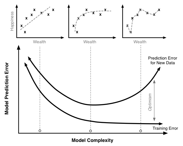
Training, optimism and true prediction error.
Increasing the model complexity will always decrease the model training error. At very high levels of complexity, we should be able to in effect perfectly predict every single point in the training data set and the training error should be near 0. Similarly, the true prediction error initially falls. The linear model without polynomial terms seems a little too simple for this data set. However, once we pass a certain point, the true prediction error starts to rise. At these high levels of complexity, the additional complexity we are adding helps us fit our training data, but it causes the model to do a worse job of predicting new data.
This is a case of overfitting the training data. In this region the model training algorithm is focusing on precisely matching random chance variability in the training set that is not present in the actual population. We can see this most markedly in the model that fits every point of the training data; clearly this is too tight a fit to the training data.
Preventing overfitting is a key to building robust and accurate prediction models. Overfitting is very easy to miss when only looking at the training error curve. To detect overfitting you need to look at the true prediction error curve. Of course, it is impossible to measure the exact true prediction curve (unless you have the complete data set for your entire population), but there are many different ways that have been developed to attempt to estimate it with great accuracy. The second section of this work will look at a variety of techniques to accurately estimate the model’s true prediction error.
An Example of the Cost of Poorly Measuring Error
Let’s look at a fairly common modeling workflow and use it to illustrate the pitfalls of using training error in place of the true prediction error 2. We’ll start by generating 100 simulated data points. Each data point has a target value we are trying to predict along with 50 different parameters. For instance, this target value could be the growth rate of a species of tree and the parameters are precipitation, moisture levels, pressure levels, latitude, longitude, etc. In this case however, we are going to generate every single data point completely randomly. Each number in the data set is completely independent of all the others, and there is no relationship between any of them.
For this data set, we create a linear regression model where we predict the target value using the fifty regression variables. Since we know everything is unrelated we would hope to find an R2 of 0. Unfortunately, that is not the case and instead we find an R2 of 0.5. That’s quite impressive given that our data is pure noise! However, we want to confirm this result so we do an F-test. This test measures the statistical significance of the overall regression to determine if it is better than what would be expected by chance. Using the F-test we find a p-value of 0.53. This indicates our regression is not significant.
If we stopped there, everything would be fine; we would throw out our model which would be the right choice (it is pure noise after all!). However, a common next step would be to throw out only the parameters that were poor predictors, keep the ones that are relatively good predictors and run the regression again. Let’s say we kept the parameters that were significant at the 25% level of which there are 21 in this example case. Then we rerun our regression.
In this second regression we would find:
- An R2 of 0.36
- A p-value of 5*10-4
- 6 parameters significant at the 5% level
Again, this data was pure noise; there was absolutely no relationship in it. But from our data we find a highly significant regression, a respectable R2 (which can be very high compared to those found in some fields like the social sciences) and 6 significant parameters!
This is quite a troubling result, and this procedure is not an uncommon one but clearly leads to incredibly misleading results. It shows how easily statistical processes can be heavily biased if care to accurately measure error is not taken.
Methods of Measuring Error
Adjusted R2
The R2 measure is by far the most widely used and reported measure of error and goodness of fit. R2 is calculated quite simply. First the proposed regression model is trained and the differences between the predicted and observed values are calculated and squared. These squared errors are summed and the result is compared to the sum of the squared errors generated using the null model. The null model is a model that simply predicts the average target value regardless of what the input values for that point are. The null model can be thought of as the simplest model possible and serves as a benchmark against which to test other models. Mathematically:
$$ R^2 = 1 — frac{Sum of Squared Errors Model}{Sum of Squared Errors Null Model} $$
R2 has very intuitive properties. When our model does no better than the null model then R2 will be 0. When our model makes perfect predictions, R2 will be 1. R2 is an easy to understand error measure that is in principle generalizable across all regression models.
Commonly, R2 is only applied as a measure of training error. This is unfortunate as we saw in the above example how you can get high R2 even with data that is pure noise. In fact there is an analytical relationship to determine the expected R2 value given a set of n observations and p parameters each of which is pure noise:
$$Eleft[R^2right]=frac{p}{n}$$
So if you incorporate enough data in your model you can effectively force whatever level of R2 you want regardless of what the true relationship is. In our illustrative example above with 50 parameters and 100 observations, we would expect an R2 of 50/100 or 0.5.
One attempt to adjust for this phenomenon and penalize additional complexity is Adjusted R2. Adjusted R2 reduces R2 as more parameters are added to the model. There is a simple relationship between adjusted and regular R2:
$$Adjusted R^2=1-(1-R^2)frac{n-1}{n-p-1}$$
Unlike regular R2, the error predicted by adjusted R2 will start to increase as model complexity becomes very high. Adjusted R2 is much better than regular R2 and due to this fact, it should always be used in place of regular R2. However, adjusted R2 does not perfectly match up with the true prediction error. In fact, adjusted R2 generally under-penalizes complexity. That is, it fails to decrease the prediction accuracy as much as is required with the addition of added complexity.
Given this, the usage of adjusted R2 can still lead to overfitting. Furthermore, adjusted R2 is based on certain parametric assumptions that may or may not be true in a specific application. This can further lead to incorrect conclusions based on the usage of adjusted R2.
Pros
- Easy to apply
- Built into most existing analysis programs
- Fast to compute
- Easy to interpret 3
Cons
- Less generalizable
- May still overfit the data
Information Theoretic Approaches
There are a variety of approaches which attempt to measure model error as how much information is lost between a candidate model and the true model. Of course the true model (what was actually used to generate the data) is unknown, but given certain assumptions we can still obtain an estimate of the difference between it and and our proposed models. For a given problem the more this difference is, the higher the error and the worse the tested model is.
Information theoretic approaches assume a parametric model. Given a parametric model, we can define the likelihood of a set of data and parameters as the, colloquially, the probability of observing the data given the parameters 4. If we adjust the parameters in order to maximize this likelihood we obtain the maximum likelihood estimate of the parameters for a given model and data set. We can then compare different models and differing model complexities using information theoretic approaches to attempt to determine the model that is closest to the true model accounting for the optimism.
The most popular of these the information theoretic techniques is Akaike’s Information Criteria (AIC). It can be defined as a function of the likelihood of a specific model and the number of parameters in that model:
$$ AIC = -2 ln(Likelihood) + 2p $$
Like other error criteria, the goal is to minimize the AIC value. The AIC formulation is very elegant. The first part ($-2 ln(Likelihood)$) can be thought of as the training set error rate and the second part ($2p$) can be though of as the penalty to adjust for the optimism.
However, in addition to AIC there are a number of other information theoretic equations that can be used. The two following examples are different information theoretic criteria with alternative derivations. In these cases, the optimism adjustment has different forms and depends on the number of sample size (n).
$$ AICc = -2 ln(Likelihood) + 2p + frac{2p(p+1)}{n-p-1} $$
$$ BIC = -2 ln(Likelihood) + p ln(n) $$
The choice of which information theoretic approach to use is a very complex one and depends on a lot of specific theory, practical considerations and sometimes even philosophical ones. This can make the application of these approaches often a leap of faith that the specific equation used is theoretically suitable to a specific data and modeling problem.
Pros
- Easy to apply
- Built into most advanced analysis programs
Cons
- Metric not comparable between different applications
- Requires a model that can generate likelihoods 5
- Various forms a topic of theoretical debate within the academic field
Holdout Set
Both the preceding techniques are based on parametric and theoretical assumptions. If these assumptions are incorrect for a given data set then the methods will likely give erroneous results. Fortunately, there exists a whole separate set of methods to measure error that do not make these assumptions and instead use the data itself to estimate the true prediction error.
The simplest of these techniques is the holdout set method. Here we initially split our data into two groups. One group will be used to train the model; the second group will be used to measure the resulting model’s error. For instance, if we had 1000 observations, we might use 700 to build the model and the remaining 300 samples to measure that model’s error.
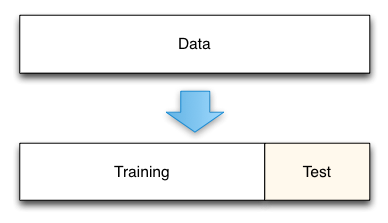
Holdout data split.
This technique is really a gold standard for measuring the model’s true prediction error. As defined, the model’s true prediction error is how well the model will predict for new data. By holding out a test data set from the beginning we can directly measure this.
The cost of the holdout method comes in the amount of data that is removed from the model training process. For instance, in the illustrative example here, we removed 30% of our data. This means that our model is trained on a smaller data set and its error is likely to be higher than if we trained it on the full data set. The standard procedure in this case is to report your error using the holdout set, and then train a final model using all your data. The reported error is likely to be conservative in this case, with the true error of the full model actually being lower. Such conservative predictions are almost always more useful in practice than overly optimistic predictions.
One key aspect of this technique is that the holdout data must truly not be analyzed until you have a final model. A common mistake is to create a holdout set, train a model, test it on the holdout set, and then adjust the model in an iterative process. If you repeatedly use a holdout set to test a model during development, the holdout set becomes contaminated. Its data has been used as part of the model selection process and it no longer gives unbiased estimates of the true model prediction error.
Pros
- No parametric or theoretic assumptions
- Given enough data, highly accurate
- Very simple to implement
- Conceptually simple
Cons
- Potential conservative bias
- Tempting to use the holdout set prior to model completion resulting in contamination
- Must choose the size of the holdout set (70%-30% is a common split)
Cross-Validation and Resampling
In some cases the cost of setting aside a significant portion of the data set like the holdout method requires is too high. As a solution, in these cases a resampling based technique such as cross-validation may be used instead.
Cross-validation works by splitting the data up into a set of n folds. So, for example, in the case of 5-fold cross-validation with 100 data points, you would create 5 folds each containing 20 data points. Then the model building and error estimation process is repeated 5 times. Each time four of the groups are combined (resulting in 80 data points) and used to train your model. Then the 5th group of 20 points that was not used to construct the model is used to estimate the true prediction error. In the case of 5-fold cross-validation you would end up with 5 error estimates that could then be averaged to obtain a more robust estimate of the true prediction error.
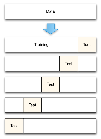
5-Fold cross-validation data split.
As can be seen, cross-validation is very similar to the holdout method. Where it differs, is that each data point is used both to train models and to test a model, but never at the same time. Where data is limited, cross-validation is preferred to the holdout set as less data must be set aside in each fold than is needed in the pure holdout method. Cross-validation can also give estimates of the variability of the true error estimation which is a useful feature. However, if understanding this variability is a primary goal, other resampling methods such as Bootstrapping are generally superior.
On important question of cross-validation is what number of folds to use. Basically, the smaller the number of folds, the more biased the error estimates (they will be biased to be conservative indicating higher error than there is in reality) but the less variable they will be. On the extreme end you can have one fold for each data point which is known as Leave-One-Out-Cross-Validation. In this case, your error estimate is essentially unbiased but it could potentially have high variance. Understanding the Bias-Variance Tradeoff is important when making these decisions. Another factor to consider is computational time which increases with the number of folds. For each fold you will have to train a new model, so if this process is slow, it might be prudent to use a small number of folds. Ultimately, it appears that, in practice, 5-fold or 10-fold cross-validation are generally effective fold sizes.
Pros
- No parametric or theoretic assumptions
- Given enough data, highly accurate
- Conceptually simple
Cons
- Computationally intensive
- Must choose the fold size
- Potential conservative bias
Making a Choice
In summary, here are some techniques you can use to more accurately measure model prediction error:
- Adjusted R2
- Information Theoretic Techniques
- Holdout Sample
- Cross-Validation and Resampling Methods
A fundamental choice a modeler must make is whether they want to rely on theoretic and parametric assumptions to adjust for the optimism like the first two methods require. Alternatively, does the modeler instead want to use the data itself in order to estimate the optimism.
Generally, the assumption based methods are much faster to apply, but this convenience comes at a high cost. First, the assumptions that underly these methods are generally wrong. How wrong they are and how much this skews results varies on a case by case basis. The error might be negligible in many cases, but fundamentally results derived from these techniques require a great deal of trust on the part of evaluators that this error is small.
Ultimately, in my own work I prefer cross-validation based approaches. Cross-validation provides good error estimates with minimal assumptions. The primary cost of cross-validation is computational intensity but with the rapid increase in computing power, this issue is becoming increasingly marginal. At its root, the cost with parametric assumptions is that even though they are acceptable in most cases, there is no clear way to show their suitability for a specific case. Thus their use provides lines of attack to critique a model and throw doubt on its results. Although cross-validation might take a little longer to apply initially, it provides more confidence and security in the resulting conclusions.
❧
In statistics, prediction error refers to the difference between the predicted values made by some model and the actual values.
Prediction error is often used in two settings:
1. Linear regression: Used to predict the value of some continuous response variable.
We typically measure the prediction error of a linear regression model with a metric known as RMSE, which stands for root mean squared error.
It is calculated as:
RMSE = √Σ(ŷi – yi)2 / n
where:
- Σ is a symbol that means “sum”
- ŷi is the predicted value for the ith observation
- yi is the observed value for the ith observation
- n is the sample size
2. Logistic Regression: Used to predict the value of some binary response variable.
One common way to measure the prediction error of a logistic regression model is with a metric known as the total misclassification rate.
It is calculated as:
Total misclassification rate = (# incorrect predictions / # total predictions)
The lower the value for the misclassification rate, the better the model is able to predict the outcomes of the response variable.
The following examples show how to calculate prediction error for both a linear regression model and a logistic regression model in practice.
Example 1: Calculating Prediction Error in Linear Regression
Suppose we use a regression model to predict the number of points that 10 players will score in a basketball game.
The following table shows the predicted points from the model vs. the actual points the players scored:

We would calculate the root mean squared error (RMSE) as:
- RMSE = √Σ(ŷi – yi)2 / n
- RMSE = √(((14-12)2+(15-15)2+(18-20)2+(19-16)2+(25-20)2+(18-19)2+(12-16)2+(12-20)2+(15-16)2+(22-16)2) / 10)
- RMSE = 4
The root mean squared error is 4. This tells us that the average deviation between the predicted points scored and the actual points scored is 4.
Related: What is Considered a Good RMSE Value?
Example 2: Calculating Prediction Error in Logistic Regression
Suppose we use a logistic regression model to predict whether or not 10 college basketball players will get drafted into the NBA.
The following table shows the predicted outcome for each player vs. the actual outcome (1 = Drafted, 0 = Not Drafted):

We would calculate the total misclassification rate as:
- Total misclassification rate = (# incorrect predictions / # total predictions)
- Total misclassification rate = 4/10
- Total misclassification rate = 40%
The total misclassification rate is 40%.
This value is quite high, which indicates that the model doesn’t do a very good job of predicting whether or not a player will get drafted.
Additional Resources
The following tutorials provide an introduction to different types of regression methods:
Introduction to Simple Linear Regression
Introduction to Multiple Linear Regression
Introduction to Logistic Regression
Machine Learning (ML) and Artificial Intelligence (AI) are integral to most businesses nowadays. Decision-makers in many sectors, e.g., banking and finance, have employed ML-algorithms to do their heavy lifting. Though it sounds like a smart move, it is imperative to make sure these models are indeed doing what is expected of them. As are employees of a bank, models are prone to making mistakes and there is always a price to pay when using ML-models. Thus the need to continuously validate these models.
Model validation is a broad field expanding several notions. In this article, we focus on prediction models. A model may be considered valid if:
- it performs well, i.e., based on some mathematical metrics such as “a small miss-classification error” in classification prediction models.
- the model is fair, i.e., not racist, sexist, homophobes, xenophobe, etc. These are cultural or legal validity aspects.
- the model is interpret-able, some experts may argue that black-box models are invalid. In such cases understanding how the model makes predictions is central.
The three validity aspects above are not exhaustive; model validation may mean different things depending on who is validating the model.
In this article, we will discuss model validation from the viewpoint of
- Most data scientists when talking about model validation will default to point.
- Hereunder, we give models details on model validation based on prediction errors.
Before making any progress, we will introduce some notations here: :
Y: represents the outcome we want to predict, let’s say something like stock prices on a given day. We will denote the predicted Y with Ŷ.
x: represents the characteristics of the outcome — we will always know x at the time of prediction. For our stock example, x can be a date, open and closing prices for that date and so on.
m: represents a prediction model, in practice, this model will often contain parameters based on estimations. Once we estimate these parameters, we then denote the model with estimated parameters with m̂ — this will differentiate m̂ from m, the model with the true parameters.
β: will represent parameters of the model m, as we already know, we will estimate β and represent it with ˆβ.
We calculate predictions as follows:
$$hat Y(x) = hat m (x) = x^that beta $$
and want the prediction error to be as small as possible. The prediction error for a prediction at predictor x is given by
$$hat Y(x)-Y^{star}$$
Y* is the outcome we want to predict that has x as characteristics. Since a prediction model is typically used to predict an outcome before it is observed, the outcome.
Y* is unknown at the time of prediction. Hence, the prediction error cannot be computed.
Recall that a prediction model is estimated by using data in the training data set (X, Y) and that Y* is an outcome at x which is assumed to be independent of the training data. The idea is that the prediction model is intended for use in predicting a future observation Y*, i.e. an observation that has yet to be realized/observed (otherwise prediction seems rather useless). Hence, Y* can never be part of the training data set.
Here we provide definitions and we show how the prediction performance of a prediction model can be evaluated from data.
Let T= (Y, X) denote the training data, from which the prediction model is built. This building process typically involves feature (characteristic) selection and parameter estimation. Below we define different types of errors used for model validation.
Test or Generalisation, out of sample Error
The test or generalization error for prediction model is given by
$$text{Err}_T = text{E}_{(Y^star,X^star)}big{(hat m(X^star)-Y^star)^2|Tbig}$$
where (Y*, X*) is independent of the training data.
The test error is conditional on the training data T. Hence, the test error evaluates the performance of the single model built from the observed training data. This is the ultimate target of the model assessment because it is exactly this prediction model that will be used in practice and applied to future predictors X* to predict Y*. The test error is defined as an average overall such future observations (Y*; X*). The test error is the most interesting error for model validation according to point 1.
Conditional Test Error in x
The conditional test error in x for a prediction model is given by
$$text{Err}_T = text{E}_{(Y^star)}big{(hat m(x)-Y^star)^2|T,xbig}$$
where Y* is an outcome at predictor x, independent of the training data.
In-sample Error
The in-sample error for a prediction model is given by
$${ text{Err}}_{inT} = frac{1}{n}sum_{i=1}^n{ text{Err}}_{T}(x_i)$$
i.e., the in-sample error is the sample average of the conditional test errors evaluated in the n training dataset observations.
Estimation of the in-sample error
We start with introducing the training error rate, which is closely related to the mean squared error in linear models.
Training error
The training error is given by
$$bar{ text{err}} = frac{1}{n}sum_{i=1}^n(Y_i – hat m (x_i))^2$$
where the (Y, x) form the training dataset which is also used for training the models.
- The training error is an overly optimistic estimate of the test error
- The training error never increases when the model becomes more complex — cannot be used directly as a model selection criterion
Model parameters are often estimated by minimising the training error (cfr. mean squared error). Hence the fitted model adapts to the training data, and therefore the training error will be an overly optimistic estimate of the test error.
Other estimators of the in-sample error are:
- The Akaike information criterion (AIC)
- Bayesian information criterion (BIC)
- Mallow’s Cp
Expected Prediction Error and Cross-Validation
The test or generalization error was defined conditionally on the training data. By averaging over the distribution of training datasets, the expected test error arises.
Expected Test Error
begin{align}
text{E}_Ttext{Err}_T &= text{E}_Tbig{text{E}_{(Y^star,X^star)}big{(hat m(X^star)-Y^star)^2|Tbig}big}\
&= text{E}_{T,Y^star,X^star}big{(hat m(X^star)-Y^star)^2big}
end{align}
The expected test error may not be of direct interest when the goal is to assess the prediction performance of a single prediction model. The expected test error averages the test errors of all models that can be built from all training datasets, and hence this may be less relevant when the interest is in evaluating one particular model that resulted from a single observed training dataset.
Also, note that building a prediction model involves both parameter estimation and feature selection. Hence the expected test error also evaluates the feature selection procedure (on average). If the expected test error is small, it is an indication that the model building process gives good predictions for future observations (Y*, X*) on average.
Estimation of the expected test error
Cross-validation
Randomly divide the training dataset into k approximately equal subsets. Train your model on k-1 of them and compute the prediction error on the kth subset. Do this in such a way that all k subsets have been used for training and for computing the prediction error. Average the prediction errors from all k subset. This is the cross-validation error.
The process of cross-validation is clearly mimicking an expected test error and not the test error. The Cross-validation is estimating the expected test error and not the test error in which we are interested in.
Conclusion
Validating prediction models based on prediction errors can get complicated very quickly due to the different types of prediction errors that exist. A data scientist that uses any of these errors during model validation should be conscious of it. Ideally, the model validation error of interest is the test error. Proxies like the in-sample and generalized test error are often used in practice — when used, their shortcomings should be clearly stated and the reason for using them should be also outlined.
If there is enough data, you could, in fact, partition your data into training, validation (for hyper-parameter tuning) and perhaps multiple testing sets. This way good estimates of the test error are possible, leading to proper model validation.
Ready to streamline your model lifecycle?
We encounter predictions in everyday life and work: what will be the high temperature tomorrow, what will be the sales of a product, what will be the price of fuel, how large will be the harvest of grain at the end of the season, and so on. Often such predictions come from authoritative sources: the weather bureau, the government, think tanks. These predictions, like those that come from our own statistical models, are likely to be somewhat off target from the actual outcome.
This chapter introduces a simple, standard way to quantify the size of prediction errors: the root mean square prediction error (RMSE). Those five words are perhaps a mouthful, but as you’ll see, “root mean square” is not such a difficult operation.
Prediction error
We often think of “error” as the result of a mistake or blunder. That’s not really the case for prediction error. Prediction models are built using the resources available to us: explanatory variables that can be measured, accessible data about previous events, our limited understanding of the mechanisms at work, and so on. Naturally, given such flaws our predictions will be imperfect. It seems harsh to call these imperfections an “error”. Nonetheless, Prediction error is the name given to the deviation between the output of our models and the way things eventually turned out in the real world.
The use we can make of a prediction depends on how large those errors are likely to be. We have to say “likely to be” because, at the time we make the prediction, we don’t know what the actual result will be. Chapter 5 introduced the idea of a prediction interval: a range of values that we believe the actual result is highly likely to be in. “Highly likely” is conventionally taken to be 95%.
It may seem mysterious how one can anticipate what an error is likely to be, but the strategy is simple. In order to guide our predictions of the future, we look at our records of the past. The data we use to train a statistical model contains the values of the response variable as well as the explanatory variables. This provides the opportunity to assess the performance of the model. First, generate prediction outputs using as inputs the values of the explanatory variables, Then, compare the prediction outputs to the actual value of the response variable.
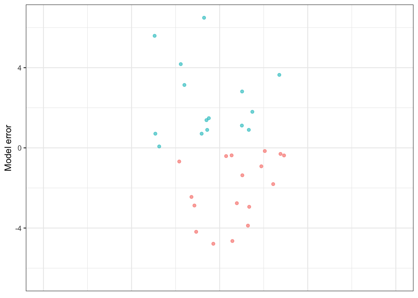
The comparison process is illustrated in Table 16.1 and, equivalently, Figure 16.1. The error is the numerical difference between the actual response value and the model output. The error is calculated from our data on a row-by-row basis: one error for each row in our data. The error will be positive when the actual response is larger than the model output, negative when the actual response is smaller, and would be zero if the actual response equals the model output.
Table 16.1: Prediction error from a model mpg ~ hp + cyl of automobile fuel economy versus engine horsepower and number of cylinders. The actual response variable, mpg, is compared to the model output to produce the error and square error.
| hp | cyl | mpg | model_output | error | square_error |
|---|---|---|---|---|---|
| 110 | 6 | 21.0 | 20.29 | 0.71 | 0.51 |
| 110 | 6 | 21.0 | 20.29 | 0.71 | 0.51 |
| 93 | 4 | 22.8 | 25.74 | -2.94 | 8.67 |
| 110 | 6 | 21.4 | 20.29 | 1.11 | 1.24 |
| 175 | 8 | 18.7 | 15.56 | 3.14 | 9.85 |
| 105 | 6 | 18.1 | 20.55 | -2.45 | 6.00 |
| … and so on for 32 rows altogether. |
Figure 16.1: A graphical presentation of Table 16.1. The data layer presents the actual values of the input and output variables. The model output is displayed in a statistics layer by a dash. The error is shown in an interval layer. To emphasize that the error can be positive or negative, color is used to show the sign.
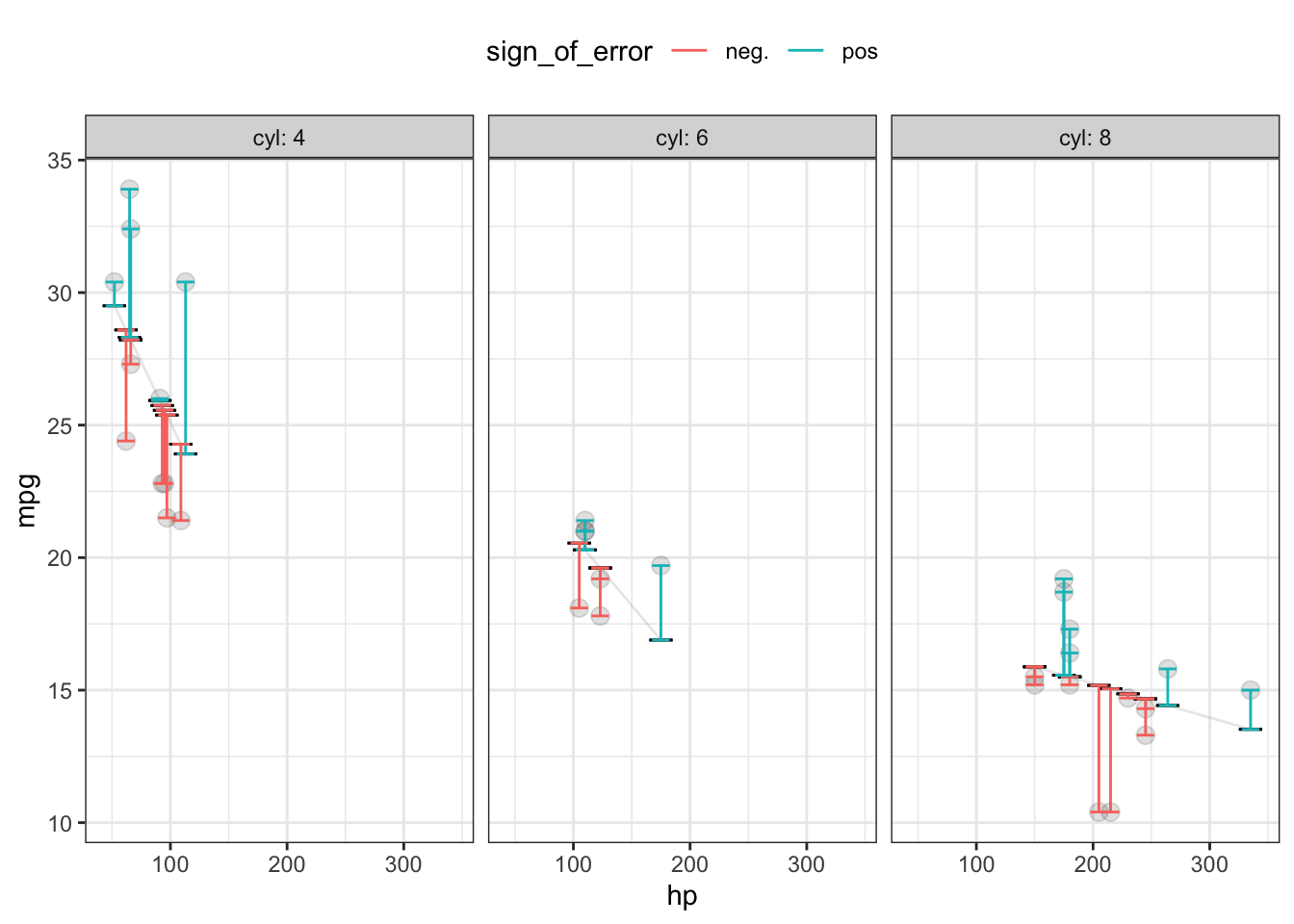
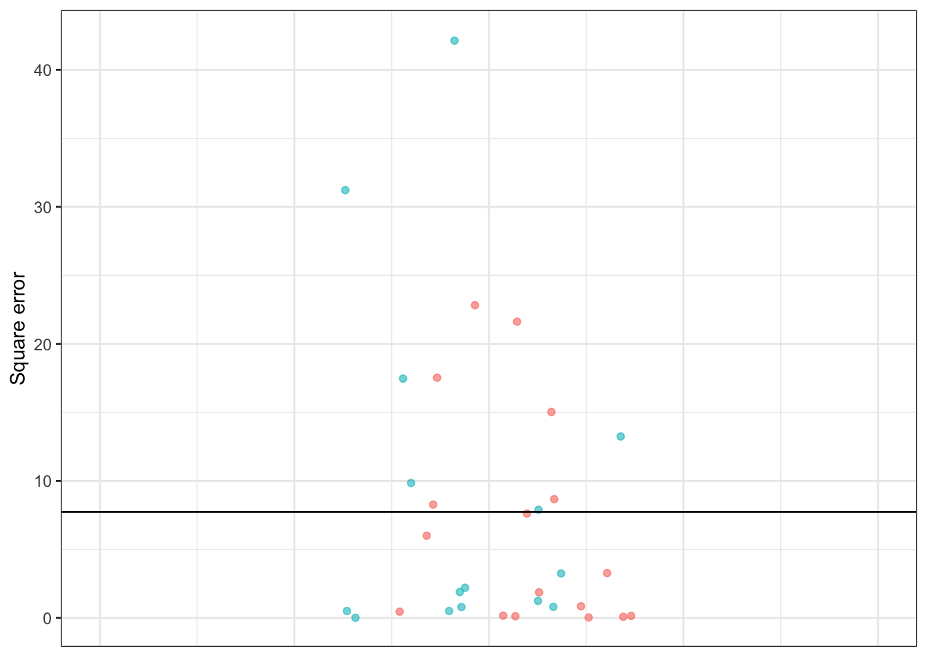
Once each row-by-row error has been found, we consolidate these errors into a single number representing an overall measure of the performance of the model. One easy way to do this is based on the square error, also shown in Table 16.1 and Figure 16.1. The squaring process turns any negative errors into positive square errors.
Figure 16.2: The prediction errors and square errors corresponding to Table 16.1 and Figure 16.1. The color shows the sign of the error. Since errors are both positive and negative in sign, overall they are centered on zero. But square errors are always positive, so the mean square error is positive.
Adding up those square errors gives the so-called sum of square errors (SSE). The SSE depends, of course, on both how large the individual errors are and how many rows there are in the data. For Table 16.1, the SSE is
247.61 miles-per-gallon.
The mean square error (MSE) is the average size of the square errors, for example dividing the sum of square errors by the number of rows in the data frame. In Table 16.1, the MSE is simply the SSE divided by the number of rows in the data frame. In Table 16.1 the MSE is 247.61 / 32 = 7.74 square-miles per square-gallon.
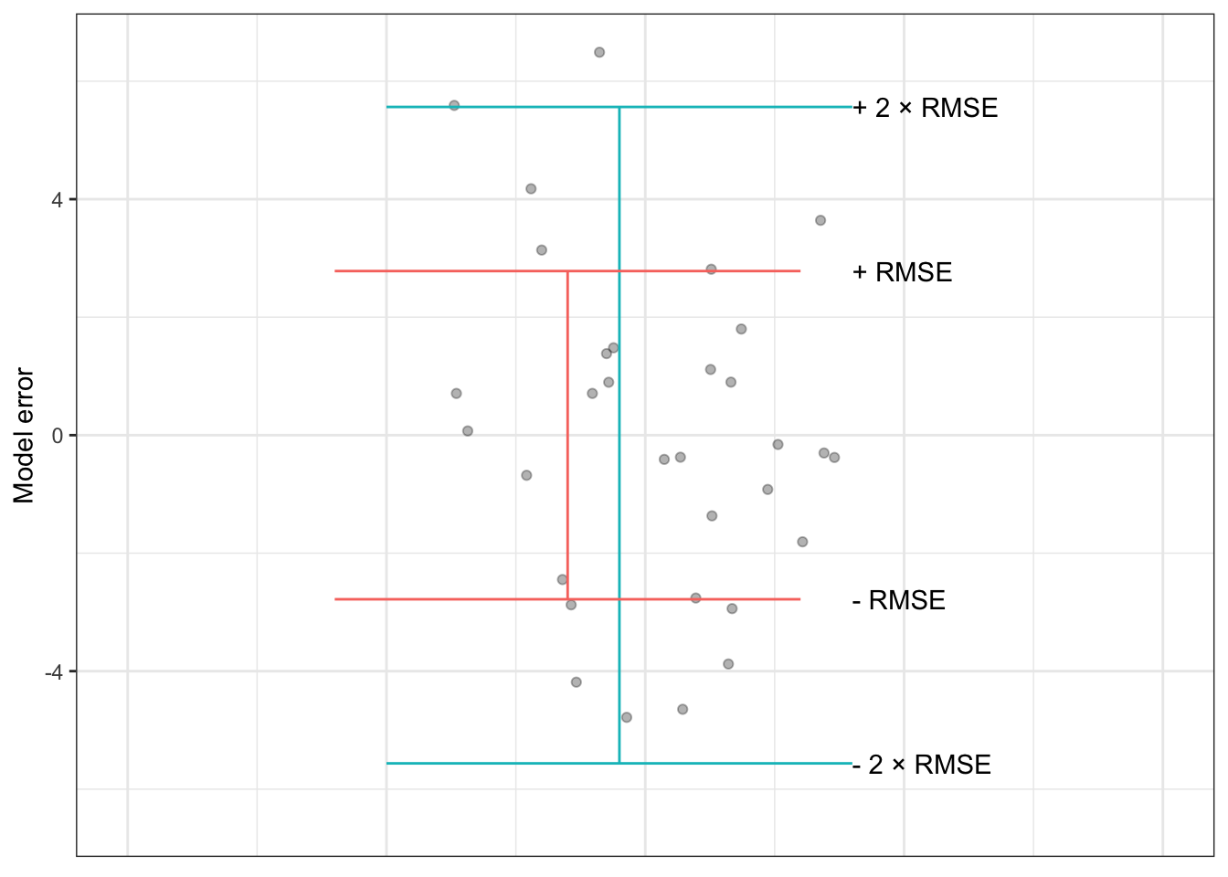
Figure 16.3: The model errors from Table 16.1 shown along with interval ± RMSE and ± 2 × RMSE. The shorter interval encompasses about 67% of the errors, the longer interval covers about 95% of the errors.
Yes, you read that right: square-miles per square-gallon. It’s important to keep track of the physical units of a prediction. These will always be the same as the physical units of the response variable. For instance, in Table 16.1, the response variable is in terms of miles-per-gallon, and so the prediction itself is in miles-per-gallon. Similarly, the prediction error, being the difference between the response value and the predicted value, is in the same units, miles-per-gallon.
Things are a little different for the square error. Squaring a quantity changes the units. For instance, squaring a quantity of 2 meters gives 4 square-meters. This is easy to understand with meters and square-meters; squaring a length produces an area. (This length-to-area conversion is the motivation behind using the word “square.”) For other quantities, such as time, the units are unfamiliar. Square the quantity “15 seconds” and you’ll get 225 square-seconds. Square the quantity “11 chickens” and you’ll get 121 square-chickens. This is not a matter of being silly, but of careful presentation of error.
A mean square error is intended to be a typical size for a square error. But the units, for instance square-miles-per-square-gallon in Table 16.1, can be hard to visualize. For this reason, most people prefer to take the square root of the mean square prediction error. This changes the units back to those of the response variable, e.g. miles-per-gallon, and is yet another way of presenting the magnitude of prediction error.
The root mean square error (RMSE) is simply the square root of the mean square prediction error. For example, in Table 16.1, the RMSE is 2.78 miles-per-gallon, which is just the square root of the MSE of 7.74 square-miles per square-gallon.
Prediction intervals and RMSE
As described in Chapter 5, predictions can be presented as a prediction interval sufficiently long to cover the large majority of the actual outputs. Another way to think about the length of the prediction interval is in terms of the magnitude typical prediction error. In order to contain the majority of actual outputs, the prediction interval ought to reach upwards beyond the typical prediction error and, similarly, reach downwards by the same amount.
The RMSE provides an operational definition of the magnitude of a typical error. So a simple way to construct a prediction interval is to fix the upper end at the prediction function output plus the RMSE and the lower end at the prediction function output minus the RMSE.
It turns out that constructing a prediction interval using ± RMSE provides a roughly 67% interval: about 67% of individual error magnitudes are within ± RMSE of the model output. In order to produce an interval covering roughly 95% of the error magnitudes, the prediction interval is usually calculated using the model output ± 2 × RMSE.
This simple way of constructing prediction intervals is not the whole story. Another component to a prediction interval is “sampling variation” in the model output. Sampling variation will be introduced in Chapter 15.
Training and testing data
When you build a prediction model, you have a data frame containing both the response variable and the explanatory variables. This data frame is sometimes called the training data, because the computer uses it to select a particular member from the modeler’s choice of the family of functions for the model, that is, to “train the model.”
In training the model, the computer picks a member of the family of functions that makes the model output as close as possible to the response values in the training data. As described in Chapter 15, if you had used a new and different data frame for training, the selected function would have been somewhat different because it would be tailored to that new data frame.
In making a prediction, you are generally interested in events that you haven’t yet seen. Naturally enough, an event you haven’t yet seen cannot be part of the training data. So the prediction error that we care about is not the prediction error calculated from the training data, but that calculated from new data. Such new data is often called testing data.
Ideally, to get a useful estimate of the size of prediction errors, you should use a testing data set rather than the training data. Of course, it can be very convenient to use the training data for testing. Sometimes no other data is available. Many statistical methods were first developed in an era when data was difficult and expensive to collect and so it was natural to use the training data for testing. A problem with doing this is that the estimated model error will tend to be smaller on the training data than on new data. To compensate for this, as described in Chapter 21, statistical methods used careful accounting, including quantities such as “degrees of freedom,” to compensate mathematically for the underestimation in the error estimate.
Nowadays, when data are plentiful, it’s feasible to split the available data into two parts: a set of rows used for training the model and another set of rows for testing the model. Even better, a method called cross validation effectively lets you use all your data for training and all your data for testing, without underestimating the prediction model’s error. Cross validation is discussed in Chapter 18.
Example: Predicting winning times in hill races
The Scottish hill race data contains four related variables: the race length, the race climb, the sex class, and the winning time in that class. Figures 10.7 and 10.8 in Section ?? show two models of the winning time:
time ~ lengthin Figure 10.7time ~ length + climb + sexin 10.8
Suppose there is a brand-new race trail introduced, with length 20 km, climb 1000 m, and that you want to predict the women’s winning time.
Using these inputs, the prediction function output is
time ~ lengthproduces output 7400 secondstime ~ length + climb + sexproduces output 7250 seconds
It’s to be expected that the two models will produce different predictions; they take different input variables.
Which of the two models is better? One indication is the size of the typical prediction error for each model. To calculate this, we use some of the data as “testing data” as in Tables 16.2 and 16.3. With the testing data (as with the training data) we already know the actual winning time of the race, so calculating the row-by-row errors and square errors for each model is easy.
Table 16.2: time ~ distance: Testing data and the model output and errors from the time ~ distance model. The mean square error is 1,861,269, giving a root mean square error of 1364 seconds.
| distance | climb | sex | time | model_output | error | square_error |
|---|---|---|---|---|---|---|
| 20.0 | 1180 | M | 7616 | 7410 | 206 | 42,436 |
| 20.0 | 1180 | W | 9290 | 7410 | 1880 | 3,534,400 |
| 19.3 | 700 | M | 4974 | 7143 | -2169 | 4,704,561 |
| 19.3 | 700 | W | 5749 | 7143 | -1394 | 1,943,236 |
| 21.0 | 520 | M | 5299 | 7791 | -2492 | 6,210,064 |
| 21.0 | 520 | W | 6101 | 7791 | -1690 | 2,856,100 |
| … and so on for 46 rows altogether. |
Table 16.3: time ~ distance + climb + sex: Testing data and the model output and errors from the time ~ distance + climb + sex model. The mean square error is 483,073 square seconds, giving a root mean square error of 695 seconds.
| distance | climb | sex | time | model_output | error | square_error |
|---|---|---|---|---|---|---|
| 20.0 | 1180 | M | 7616 | 6422 | 1194 | 1,425,636 |
| 20.0 | 1180 | W | 9290 | 7856 | 1434 | 2,056,356 |
| 19.3 | 700 | M | 4974 | 5360 | -386 | 148,996 |
| 19.3 | 700 | W | 5749 | 6525 | -776 | 602,176 |
| 21.0 | 520 | M | 5299 | 5341 | -42 | 1,764 |
| 21.0 | 520 | W | 6101 | 6488 | -387 | 149,769 |
| … and so on for 46 rows altogether. |
Using the testing data, we find that the root mean square error is
time ~ lengthhas RMSE 1364 secondstime ~ length + climb + sexhas RMSE 695 seconds
Clearly, the time ~ length + climb + sex model produces better predictions than the simpler time ~ length model.
The race is run. The women’s winning time turns out to be 8034 sec. Were the predictions right?
Obviously both predictions, 7250 and 7400 secs, were off. You would hardly expect such simple models to capture all the relevant aspects of the race (the weather? the trail surface? whether the climb is gradual throughout or particularly steep in one place? the abilities of other competitors). So it’s not a question of the prediction being right on target but of how far off the predictions were. This is easy to calculate: the length-only prediction (7400 sec) was low by 634 sec; the length-climb-sex prediction was low by 784 sec.
If the time ~ distance + climb + sex model has an RMSE that is much smaller than the RMSE for the time ~ distance model, why is it that time ~ distance had a somewhat better error in the actual race? Just because the typical error is smaller doesn’t mean that, in every instance, the actual error will be smaller.
Example: Exponentially cooling water
Back in Figure ??, we displayed data on temperature versus time data of a cup of cooling water. To model the relationship between temperature and time, we used a flexible function from the linear family. A physicist might point out that cooling often follows an exponential pattern and that a better family of functions would be the exponentials. Although exponentials are not commonly used in statistical modeling, it’s perfectly feasible to fit a function from that family to the data. The results are shown in Figure 16.4 for two different exponential functions, the flexible linear function of Figure ??, and a super-flexible linear function.
Figure 16.4: The temperature of initially boiling water as it cools over time in a cup. The thin lines show various functions fitted to the data: a stiff linear model, a flexible linear model, a special-purpose model of exponential decay.
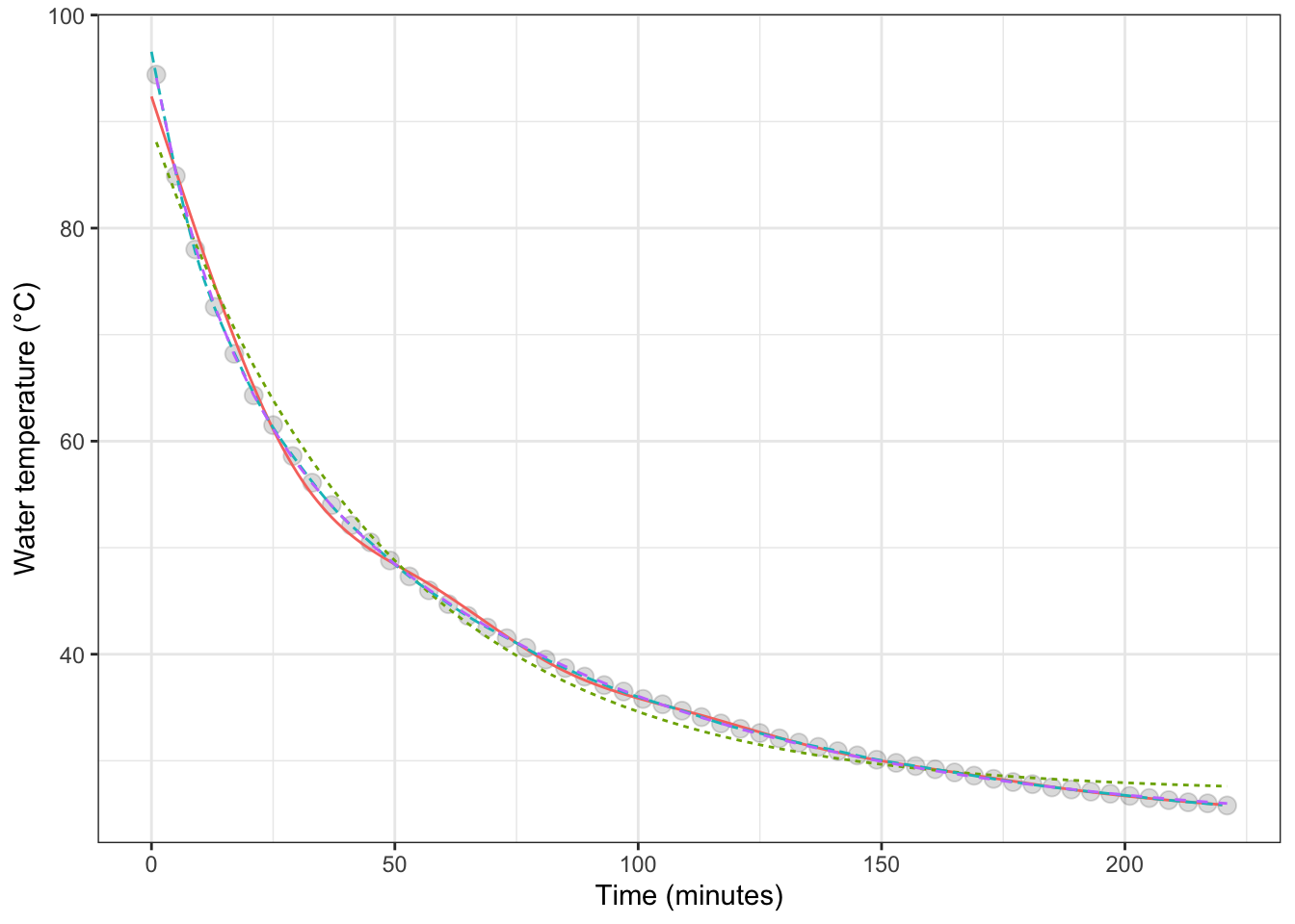
Figure 16.5: The model error – that is, the difference between the measured data and the model values – for each of the cooling water models shown in Figure 16.4.
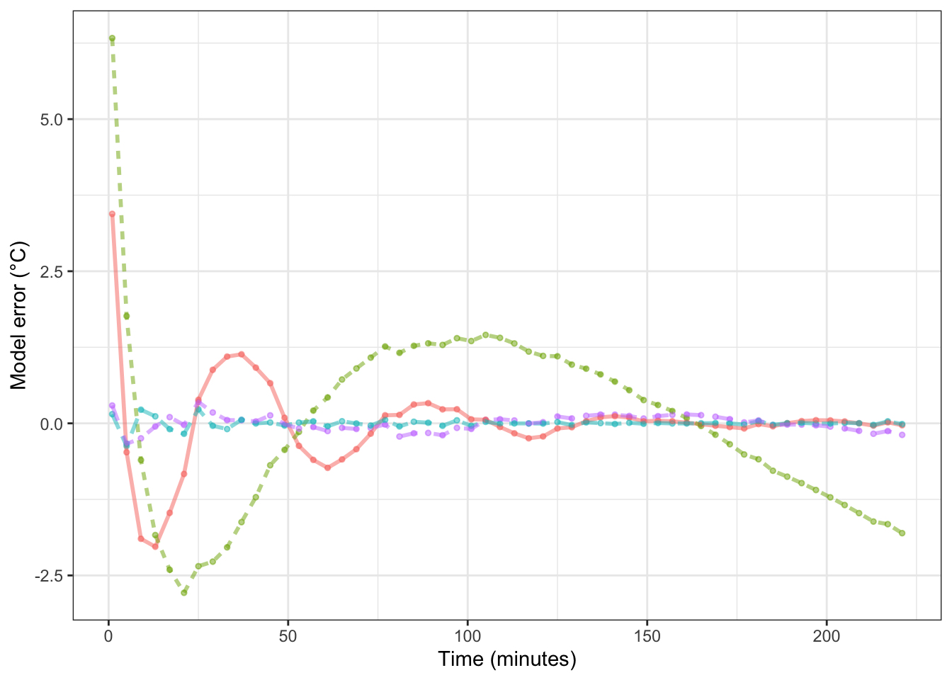
Table 16.4: The root mean square error (RMSE) for four different models of the temperature of water as it cools. The training data, not independent testing data, was used for the RMSE calculation
| model | RMSE |
|---|---|
| super flexible linear function | 0.0800 |
| two exponentials | 0.1309 |
| flexible linear function | 0.7259 |
| single exponential | 1.5003 |
To judge from solely from the RMSE, the super flexible linear function model is the best. In Chapter 18 we’ll examine the extent to which that result is due to using the training data for calculating the RMSE.
Keep in mind, though, that whether a model is good depends on the purpose for which it is being made. For a physicist, the purpose of building such a model would be to examine the physical mechanisms through which water cools. A one-exponential model corresponds to the water cooling because it is in contact with one other medium, such as the cup holding the water. A two-exponential model allows for the water to be in contact with two, different media: a fast process involving the cup and a slow process involving the room air, for instance. The RMSE for the two-exponential model is much smaller than for the one-exponential model, providing evidence that there are at least two, separate cooling mechanisms at work.