From Wikipedia, the free encyclopedia
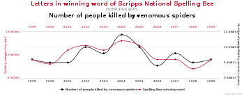
An example of a coincidence produced by data dredging (showing a correlation between the number of letters in a spelling bee’s winning word and the number of people in the United States killed by venomous spiders). Given a large enough pool of variables for the same time period, it is possible to find a pair of graphs that show a correlation with no causation.
In statistics, the multiple comparisons, multiplicity or multiple testing problem occurs when one considers a set of statistical inferences simultaneously[1] or infers a subset of parameters selected based on the observed values.[2]
The more inferences are made, the more likely erroneous inferences become. Several statistical techniques have been developed to address that problem, typically by requiring a stricter significance threshold for individual comparisons, so as to compensate for the number of inferences being made.
History[edit]
The problem of multiple comparisons received increased attention in the 1950s with the work of statisticians such as Tukey and Scheffé. Over the ensuing decades, many procedures were developed to address the problem. In 1996, the first international conference on multiple comparison procedures took place in Israel.[3]
Definition[edit]
Multiple comparisons arise when a statistical analysis involves multiple simultaneous statistical tests, each of which has a potential to produce a «discovery.» A stated confidence level generally applies only to each test considered individually, but often it is desirable to have a confidence level for the whole family of simultaneous tests.[4] Failure to compensate for multiple comparisons can have important real-world consequences, as illustrated by the following examples:
- Suppose the treatment is a new way of teaching writing to students, and the control is the standard way of teaching writing. Students in the two groups can be compared in terms of grammar, spelling, organization, content, and so on. As more attributes are compared, it becomes increasingly likely that the treatment and control groups will appear to differ on at least one attribute due to random sampling error alone.
- Suppose we consider the efficacy of a drug in terms of the reduction of any one of a number of disease symptoms. As more symptoms are considered, it becomes increasingly likely that the drug will appear to be an improvement over existing drugs in terms of at least one symptom.
In both examples, as the number of comparisons increases, it becomes more likely that the groups being compared will appear to differ in terms of at least one attribute. Our confidence that a result will generalize to independent data should generally be weaker if it is observed as part of an analysis that involves multiple comparisons, rather than an analysis that involves only a single comparison.
For example, if one test is performed at the 5% level and the corresponding null hypothesis is true, there is only a 5% risk of incorrectly rejecting the null hypothesis. However, if 100 tests are each conducted at the 5% level and all corresponding null hypotheses are true, the expected number of incorrect rejections (also known as false positives or Type I errors) is 5. If the tests are statistically independent from each other, the probability of at least one incorrect rejection is approximately 99.4%.
The multiple comparisons problem also applies to confidence intervals. A single confidence interval with a 95% coverage probability level will contain the true value of the parameter in 95% of samples. However, if one considers 100 confidence intervals simultaneously, each with 95% coverage probability, the expected number of non-covering intervals is 5. If the intervals are statistically independent from each other, the probability that at least one interval does not contain the population parameter is 99.4%.
Techniques have been developed to prevent the inflation of false positive rates and non-coverage rates that occur with multiple statistical tests.
Classification of multiple hypothesis tests[edit]
The following table defines the possible outcomes when testing multiple null hypotheses.
Suppose we have a number m of null hypotheses, denoted by: H1, H2, …, Hm.
Using a statistical test, we reject the null hypothesis if the test is declared significant. We do not reject the null hypothesis if the test is non-significant.
Summing each type of outcome over all Hi yields the following random variables:
| Null hypothesis is true (H0) | Alternative hypothesis is true (HA) | Total | |
|---|---|---|---|
| Test is declared significant | V | S | R |
| Test is declared non-significant | U | T | 
|
| Total | 
|

|
m |
In m hypothesis tests of which are true null hypotheses, R is an observable random variable, and S, T, U, and V are unobservable random variables.
Controlling procedures[edit]
Probability that at least one null hypothesis is wrongly rejected, for  , as a function of the number of independent tests
  .
.
If m independent comparisons are performed, the family-wise error rate (FWER), is given by

Hence, unless the tests are perfectly positively dependent (i.e., identical),  increases as the number of comparisons increases.
If we do not assume that the comparisons are independent, then we can still say:

which follows from Boole’s inequality. Example: 
There are different ways to assure that the family-wise error rate is at most . The most conservative method, which is free of dependence and distributional assumptions, is the Bonferroni correction  . A marginally less conservative correction can be obtained by solving the equation for the family-wise error rate of independent comparisons for
  . This yields
  , which is known as the Šidák correction. Another procedure is the Holm–Bonferroni method, which uniformly delivers more power than the simple Bonferroni correction, by testing only the lowest p-value (
 ) against the strictest criterion, and the higher p-values (
 ) against progressively less strict criteria.[5]
 .
.
For continuous problems, one can employ Bayesian logic to compute from the prior-to-posterior volume ratio. Continuous generalizations of the Bonferroni and Šidák correction are presented in.[6]
Multiple testing correction[edit]
Multiple testing correction refers to making statistical tests more stringent in order to counteract the problem of multiple testing. The best known such adjustment is the Bonferroni correction, but other methods have been developed. Such methods are typically designed to control the family-wise error rate or the false discovery rate.
Large-scale multiple testing[edit]
Traditional methods for multiple comparisons adjustments focus on correcting for modest numbers of comparisons, often in an analysis of variance. A different set of techniques have been developed for «large-scale multiple testing», in which thousands or even greater numbers of tests are performed. For example, in genomics, when using technologies such as microarrays, expression levels of tens of thousands of genes can be measured, and genotypes for millions of genetic markers can be measured. Particularly in the field of genetic association studies, there has been a serious problem with non-replication — a result being strongly statistically significant in one study but failing to be replicated in a follow-up study. Such non-replication can have many causes, but it is widely considered that failure to fully account for the consequences of making multiple comparisons is one of the causes.[7] It has been argued that advances in measurement and information technology have made it far easier to generate large datasets for exploratory analysis, often leading to the testing of large numbers of hypotheses with no prior basis for expecting many of the hypotheses to be true. In this situation, very high false positive rates are expected unless multiple comparisons adjustments are made.
For large-scale testing problems where the goal is to provide definitive results, the family-wise error rate remains the most accepted parameter for ascribing significance levels to statistical tests. Alternatively, if a study is viewed as exploratory, or if significant results can be easily re-tested in an independent study, control of the false discovery rate (FDR)[8][9][10] is often preferred. The FDR, loosely defined as the expected proportion of false positives among all significant tests, allows researchers to identify a set of «candidate positives» that can be more rigorously evaluated in a follow-up study.[11]
The practice of trying many unadjusted comparisons in the hope of finding a significant one is a known problem, whether applied unintentionally or deliberately, is sometimes called «p-hacking.»[12][13]
Assessing whether any alternative hypotheses are true[edit]

A normal quantile plot for a simulated set of test statistics that have been standardized to be Z-scores under the null hypothesis. The departure of the upper tail of the distribution from the expected trend along the diagonal is due to the presence of substantially more large test statistic values than would be expected if all null hypotheses were true. The red point corresponds to the fourth largest observed test statistic, which is 3.13, versus an expected value of 2.06. The blue point corresponds to the fifth smallest test statistic, which is -1.75, versus an expected value of -1.96. The graph suggests that it is unlikely that all the null hypotheses are true, and that most or all instances of a true alternative hypothesis result from deviations in the positive direction.
A basic question faced at the outset of analyzing a large set of testing results is whether there is evidence that any of the alternative hypotheses are true. One simple meta-test that can be applied when it is assumed that the tests are independent of each other is to use the Poisson distribution as a model for the number of significant results at a given level α that would be found when all null hypotheses are true.[citation needed] If the observed number of positives is substantially greater than what should be expected, this suggests that there are likely to be some true positives among the significant results. For example, if 1000 independent tests are performed, each at level α = 0.05, we expect 0.05 × 1000 = 50 significant tests to occur when all null hypotheses are true. Based on the Poisson distribution with mean 50, the probability of observing more than 61 significant tests is less than 0.05, so if more than 61 significant results are observed, it is very likely that some of them correspond to situations where the alternative hypothesis holds. A drawback of this approach is that it overstates the evidence that some of the alternative hypotheses are true when the test statistics are positively correlated, which commonly occurs in practice.[citation needed]. On the other hand, the approach remains valid even in the presence of correlation among the test statistics, as long as the Poisson distribution can be shown to provide a good approximation for the number of significant results. This scenario arises, for instance, when mining significant frequent itemsets from transactional datasets. Furthermore, a careful two stage analysis can bound the FDR at a pre-specified level.[14]
Another common approach that can be used in situations where the test statistics can be standardized to Z-scores is to make a normal quantile plot of the test statistics. If the observed quantiles are markedly more dispersed than the normal quantiles, this suggests that some of the significant results may be true positives.[citation needed]
See also[edit]
- q-value
- Key concepts
- Family-wise error rate
- False positive rate
- False discovery rate (FDR)
- False coverage rate (FCR)
- Interval estimation
- Post-hoc analysis
- Experimentwise error rate
- Statistical hypothesis testing
- General methods of alpha adjustment for multiple comparisons
- Closed testing procedure
- Bonferroni correction
- Boole–Bonferroni bound
- Duncan’s new multiple range test
- Holm–Bonferroni method
- Harmonic mean p-value procedure
- Benjamini–Hochberg procedure
- Related concepts
- Testing hypotheses suggested by the data
- Texas sharpshooter fallacy
- Model selection
- Look-elsewhere effect
- Data dredging
References[edit]
- ^ Miller, R.G. (1981). Simultaneous Statistical Inference 2nd Ed. Springer Verlag New York. ISBN 978-0-387-90548-8.
- ^ Benjamini, Y. (2010). «Simultaneous and selective inference: Current successes and future challenges». Biometrical Journal. 52 (6): 708–721. doi:10.1002/bimj.200900299. PMID 21154895. S2CID 8806192.
- ^ «Home». mcp-conference.org.
- ^ Kutner, Michael; Nachtsheim, Christopher; Neter, John; Li, William (2005). Applied Linear Statistical Models. pp. 744–745. ISBN 9780072386882.
- ^ Aickin, M; Gensler, H (May 1996). «Adjusting for multiple testing when reporting research results: the Bonferroni vs Holm methods». Am J Public Health. 86 (5): 726–728. doi:10.2105/ajph.86.5.726. PMC 1380484. PMID 8629727.
- ^ Bayer, Adrian E.; Seljak, Uroš (2020). «The look-elsewhere effect from a unified Bayesian and frequentist perspective». Journal of Cosmology and Astroparticle Physics. 2020 (10): 009. arXiv:2007.13821. Bibcode:2020JCAP…10..009B. doi:10.1088/1475-7516/2020/10/009. S2CID 220830693.
- ^ Qu, Hui-Qi; Tien, Matthew; Polychronakos, Constantin (2010-10-01). «Statistical significance in genetic association studies». Clinical and Investigative Medicine. 33 (5): E266–E270. ISSN 0147-958X. PMC 3270946. PMID 20926032.
- ^ Benjamini, Yoav; Hochberg, Yosef (1995). «Controlling the false discovery rate: a practical and powerful approach to multiple testing». Journal of the Royal Statistical Society, Series B. 57 (1): 125–133. JSTOR 2346101.
- ^ Storey, JD; Tibshirani, Robert (2003). «Statistical significance for genome-wide studies». PNAS. 100 (16): 9440–9445. Bibcode:2003PNAS..100.9440S. doi:10.1073/pnas.1530509100. JSTOR 3144228. PMC 170937. PMID 12883005.
- ^ Efron, Bradley; Tibshirani, Robert; Storey, John D.; Tusher, Virginia (2001). «Empirical Bayes analysis of a microarray experiment». Journal of the American Statistical Association. 96 (456): 1151–1160. doi:10.1198/016214501753382129. JSTOR 3085878. S2CID 9076863.
- ^ Noble, William S. (2009-12-01). «How does multiple testing correction work?». Nature Biotechnology. 27 (12): 1135–1137. doi:10.1038/nbt1209-1135. ISSN 1087-0156. PMC 2907892. PMID 20010596.
- ^ Young, S. S., Karr, A. (2011). «Deming, data and observational studies» (PDF). Significance. 8 (3): 116–120. doi:10.1111/j.1740-9713.2011.00506.x.
{{cite journal}}: CS1 maint: multiple names: authors list (link) - ^
Smith, G. D., Shah, E. (2002). «Data dredging, bias, or confounding». BMJ. 325 (7378): 1437–1438. doi:10.1136/bmj.325.7378.1437. PMC 1124898. PMID 12493654.{{cite journal}}: CS1 maint: multiple names: authors list (link) - ^ Kirsch, A; Mitzenmacher, M; Pietracaprina, A; Pucci, G; Upfal, E; Vandin, F (June 2012). «An Efficient Rigorous Approach for Identifying Statistically Significant Frequent Itemsets». Journal of the ACM. 59 (3): 12:1–12:22. arXiv:1002.1104. doi:10.1145/2220357.2220359.
Further reading[edit]
- F. Betz, T. Hothorn, P. Westfall (2010), Multiple Comparisons Using R, CRC Press
- S. Dudoit and M. J. van der Laan (2008), Multiple Testing Procedures with Application to Genomics, Springer
- Farcomeni, A. (2008). «A Review of Modern Multiple Hypothesis Testing, with particular attention to the false discovery proportion». Statistical Methods in Medical Research. 17 (4): 347–388. doi:10.1177/0962280206079046. hdl:11573/142139. PMID 17698936. S2CID 12777404.
- Phipson, B.; Smyth, G. K. (2010). «Permutation P-values Should Never Be Zero: Calculating Exact P-values when Permutations are Randomly Drawn». Statistical Applications in Genetics and Molecular Biology. 9: Article39. arXiv:1603.05766. doi:10.2202/1544-6115.1585. PMID 21044043. S2CID 10735784.
- P. H. Westfall and S. S. Young (1993), Resampling-based Multiple Testing: Examples and Methods for p-Value Adjustment, Wiley
- P. Westfall, R. Tobias, R. Wolfinger (2011) Multiple comparisons and multiple testing using SAS, 2nd edn, SAS Institute
- A gallery of examples of implausible correlations sourced by data dredging
In statistics, the multiple comparisons or multiple testing problem occurs when one considers a set of statistical inferences simultaneously.[1] or infer on selected parameters only, where the selection depends on the observed values.[2] Errors in inference, including confidence intervals that fail to include their corresponding population parameters or hypothesis tests that incorrectly reject the null hypothesis are more likely to occur when one considers the set as a whole. Several statistical techniques have been developed to prevent this from happening, allowing significance levels for single and multiple comparisons to be directly compared. These techniques generally require a stronger level of evidence to be observed in order for an individual comparison to be deemed «significant», so as to compensate for the number of inferences being made.
History
The interest in problem of multiple comparisons began in 1950’s with the work of Tukey and Scheffé. The interest increased for about two decades and then came a decline. Some even thought that the field was dead. However, the field was actually alive and more and more ideas were presented as the answer to the needs of medical statistics. The new methods and procedures came out: Closed testing procedure (Marcus et al., 1976),Holm–Bonferroni method (1979). Later, in 1980’s the issue of multiple comparisons came back. Books were published Hochberg and Tamhane (1987),Westfall and Young (1993),and Hsu (1996). At 1995 the work on False discovery rate and other new ideas had begun. Later, in 1996, the first conference on multiple comparisons took place in Israel. This meeting of researchers was followed by such conferences around the world: Berlin (2000), Bethesda (2002),
Shanghai (2005), Vienna ( 2007), and Tokyo ( 2009). All these reflect an acceleration of increase of interest in multiple comparisons.[3]
The problem
The term «comparisons» in multiple comparisons typically refers to comparisons of two groups, such as a treatment group and a control group. «Multiple comparisons» arise when a statistical analysis encompasses a number of formal comparisons, with the presumption that attention will focus on the strongest differences among all comparisons that are made. Failure to compensate for multiple comparisons can have important real-world consequences, as illustrated by the following examples.
- Suppose the treatment is a new way of teaching writing to students, and the control is the standard way of teaching writing. Students in the two groups can be compared in terms of grammar, spelling, organization, content, and so on. As more attributes are compared, it becomes more likely that the treatment and control groups will appear to differ on at least one attribute by random chance alone.
- Suppose we consider the efficacy of a drug in terms of the reduction of any one of a number of disease symptoms. As more symptoms are considered, it becomes more likely that the drug will appear to be an improvement over existing drugs in terms of at least one symptom.
- Suppose we consider the safety of a drug in terms of the occurrences of different types of side effects. As more types of side effects are considered, it becomes more likely that the new drug will appear to be less safe than existing drugs in terms of at least one side effect.
In all three examples, as the number of comparisons increases, it becomes more likely that the groups being compared will appear to differ in terms of at least one attribute. However a difference between the groups is only meaningful if it generalizes to an independent sample of data (e.g. to an independent set of people treated with the same drug). Our confidence that a result will generalize to independent data should generally be weaker if it is observed as part of an analysis that involves multiple comparisons, rather than an analysis that involves only a single comparison.
For example, if one test is performed at the 5% level, there is only a 5% chance of incorrectly rejecting the null hypothesis if the null hypothesis is true. However, for 100 tests where all null hypotheses are true, the expected number of incorrect rejections is 5. If the tests are independent, the probability of at least one incorrect rejection is 99.4%. These errors are called false positives or Type I errors.
The problem also occurs for confidence intervals, note that a single confidence interval with 95% coverage probability level will likely contain the population parameter it is meant to contain, i.e. in the long run 95% of confidence intervals built in that way will contain the true population parameter. However, if one considers 100 confidence intervals simultaneously, with coverage probability 0.95 each, it is highly likely that at least one interval will not contain its population parameter. The expected number of such non-covering intervals is 5, and if the intervals are independent, the probability that at least one interval does not contain the population parameter is 99.4%.
Techniques have been developed to control the false positive error rate associated with performing multiple statistical tests. Similarly, techniques have been developed to adjust confidence intervals so that the probability of at least one of the intervals not covering its target value is controlled.
Example: Flipping coins
For example, one might declare that a coin was biased if in 10 flips it landed heads at least 9 times. Indeed, if one assumes as a null hypothesis that the coin is fair, then the probability that a fair coin would come up heads at least 9 out of 10 times is (10 + 1) × (1/2)10 = 0.0107. This is relatively unlikely, and under statistical criteria such as p-value < 0.05, one would declare that the null hypothesis should be rejected — i.e., the coin is unfair.
A multiple-comparisons problem arises if one wanted to use this test (which is appropriate for testing the fairness of a single coin), to test the fairness of many coins. Imagine if one was to test 100 fair coins by this method. Given that the probability of a fair coin coming up 9 or 10 heads in 10 flips is 0.0107, one would expect that in flipping 100 fair coins ten times each, to see a particular (i.e., pre-selected) coin come up heads 9 or 10 times would still be very unlikely, but seeing any coin behave that way, without concern for which one, would be more likely than not. Precisely, the likelihood that all 100 fair coins are identified as fair by this criterion is (1 − 0.0107)100 ≈ 0.34. Therefore the application of our single-test coin-fairness criterion to multiple comparisons would be more likely to falsely identify at least one fair coin as unfair.
What can be done
For hypothesis testing, the problem of multiple comparisons (also known as the multiple testing problem) results from the increase in type I error that occurs when statistical tests are used repeatedly. If n independent comparisons are performed, the experiment-wide significance level α, also termed FWER for familywise error rate, is given by
 .
.

Hence, unless the tests are perfectly dependent, α increases as the number of comparisons increases.
If we do not assume that the comparisons are independent, then we can still say:

which follows from Boole’s inequality. Example: 
There are different ways to assure that the familywise error rate is at most . The most coservative, but free of independency and distribution assumptions method, is known as the Bonferroni correction  . A more sensitive correction can be obtained by solving the equation for the familywise error rate of
  independent comparisons for . This yields
  , which is known as the Šidák correction. Another procedure is the Holm–Bonferroni method which is uniformly more powerful than the Bonferroni correction.[4]
 .
.
Methods
Multiple testing correction refers to re-calculating probabilities obtained from a statistical test which was repeated multiple times. In order to retain a prescribed familywise error rate α in an analysis involving more than one comparison, the error rate for each comparison must be more stringent than α. Boole’s inequality implies that if each test is performed to have type I error rate α/n, the total error rate will not exceed α. This is called the Bonferroni correction, and is one of the most commonly used approaches for multiple comparisons.
In some situations, the Bonferroni correction is substantially conservative, i.e., the actual familywise error rate is much less than the prescribed level α. This occurs when the test statistics are highly dependent (in the extreme case where the tests are perfectly dependent, the familywise error rate with no multiple comparisons adjustment and the per-test error rates are identical). For example, in fMRI analysis,[5][6] tests are done on over 100000 voxels in the brain. The Bonferroni method would require p-values to be smaller than .05/100000 to declare significance. Since adjacent voxels tend to be highly correlated, this threshold is generally too stringent.
Because simple techniques such as the Bonferroni method can be too conservative, there has been a great deal of attention paid to developing better techniques, such that the overall rate of false positives can be maintained without inflating the rate of false negatives unnecessarily. Such methods can be divided into general categories:
- Methods where total alpha can be proved to never exceed 0.05 (or some other chosen value) under any conditions. These methods provide «strong» control against Type I error, in all conditions including a partially correct null hypothesis.
- Methods where total alpha can be proved not to exceed 0.05 except under certain defined conditions.
- Methods which rely on an omnibus test before proceeding to multiple comparisons. Typically these methods require a significant ANOVA/Tukey’s range test before proceeding to multiple comparisons. These methods have «weak» control of Type I error.
- Empirical methods, which control the proportion of Type I errors adaptively, utilizing correlation and distribution characteristics of the observed data.
The advent of computerized resampling methods, such as bootstrapping and Monte Carlo simulations, has given rise to many techniques in the latter category. In some cases where exhaustive permutation resampling is performed, these tests provide exact, strong control of Type I error rates; in other cases, such as bootstrap sampling, they provide only approximate control.
Post-hoc testing of ANOVAs
Multiple comparison procedures are commonly used in an analysis of variance after obtaining a significant omnibus test result, like the ANOVA F-test. The significant ANOVA result suggests rejecting the global null hypothesis H0 that the means are the same across the groups being compared. Multiple comparison procedures are then used to determine which means differ. In a one-way ANOVA involving K group means, there are K(K − 1)/2 pairwise comparisons.
A number of methods have been proposed for this problem, some of which are:
- Single-step procedures
- Tukey–Kramer method (Tukey’s HSD) (1951)
- Scheffe method (1953)
- Multi-step procedures based on Studentized range statistic
- Duncan’s new multiple range test (1955)
- The Nemenyi test is similar to Tukey’s range test in ANOVA.
- The Bonferroni–Dunn test allows comparisons, controlling the familywise error rate.Template:Vague
- Student Newman-Keuls post-hoc analysis
- Dunnett’s test (1955) for comparison of number of treatments to a single control group.
Choosing the most appropriate multiple-comparison procedure for your specific situation is not easy. Many tests are available, and they differ in a number of ways.[7]
For example,if the variances of the groups being compared are similar, the Tukey–Kramer method is generally viewed as performing optimally or near-optimally in a broad variety of circumstances.[8] The situation where the variance of the groups being compared differ is more complex, and different methods perform well in different circumstances.
The Kruskal–Wallis test is the non-parametric alternative to ANOVA. Multiple comparisons can be done using pairwise comparisons (for example using Wilcoxon rank sum tests) and using a correction to determine if the post-hoc tests are significant (for example a Bonferroni correction).
Large-scale multiple testing
Traditional methods for multiple comparisons adjustments focus on correcting for modest numbers of comparisons, often in an analysis of variance. A different set of techniques have been developed for «large-scale multiple testing,» in which thousands or even greater numbers of tests are performed. For example, in genomics, when using technologies such as microarrays, expression levels of tens of thousands of genes can be measured, and genotypes for millions of genetic markers can be measured. Particularly in the field of genetic association studies, there has been a serious problem with non-replication — a result being strongly statistically significant in one study but failing to be replicated in a follow-up study. Such non-replication can have many causes, but it is widely considered that failure to fully account for the consequences of making multiple comparisons is one of the causes.
In different branches of science, multiple testing is handled in different ways. It has been argued that if statistical tests are only performed when there is a strong basis for expecting the result to be true, multiple comparisons adjustments are not necessary.[9] It has also been argued that use of multiple testing corrections is an inefficient way to perform empirical research, since multiple testing adjustments control false positives at the potential expense of many more false negatives. On the other hand, it has been argued that advances in measurement and information technology have made it far easier to generate large datasets for exploratory analysis, often leading to the testing of large numbers of hypotheses with no prior basis for expecting many of the hypotheses to be true. In this situation, very high false positive rates are expected unless multiple comparisons adjustments are made.[10]
For large-scale testing problems where the goal is to provide definitive results, the familywise error rate remains the most accepted parameter for ascribing significance levels to statistical tests. Alternatively, if a study is viewed as exploratory, or if significant results can be easily re-tested in an independent study, control of the false discovery rate (FDR)[11][12][13] is often preferred. The FDR, defined as the expected proportion of false positives among all significant tests, allows researchers to identify a set of «candidate positives,» of which a high proportion are likely to be true. The false positives within the candidate set can then be identified in a follow-up study.
Assessing whether any alternative hypotheses are true
A normal quantile plot for a simulated set of test statistics that have been standardized to be Z-scores under the null hypothesis. The departure of the upper tail of the distribution from the expected trend along the diagonal is due to the presence of substantially more large test statistic values than would be expected if all null hypotheses were true. The red point corresponds to the fourth largest observed test statistic, which is 3.13, versus an expected value of 2.06. The blue point corresponds to the fifth smallest test statistic, which is -1.75, versus an expected value of -1.96. The graph suggests that it is unlikely that all the null hypotheses are true, and that most or all instances of a true alternative hypothesis result from deviations in the positive direction.
A basic question faced at the outset of analyzing a large set of testing results is whether there is evidence that any of the alternative hypotheses are true. One simple meta-test that can be applied when it is assumed that the tests are independent of each other is to use the Poisson distribution as a model for the number of significant results at a given level α that would be found when all null hypotheses are true. If the observed number of positives is substantially greater than what should be expected, this suggests that there are likely to be some true positives among the significant results. For example, if 1000 independent tests are performed, each at level α = 0.05, we expect 50 significant tests to occur when all null hypotheses are true. Based on the Poisson distribution with mean 50, the probability of observing more than 61 significant tests is less than 0.05, so if we observe more than 61 significant results, it is very likely that some of them correspond to situations where the alternative hypothesis holds. A drawback of this approach is that it over-states the evidence that some of the alternative hypotheses are true when the test statistics are positively correlated, which commonly occurs in practice. Template:Cn
Another common approach that can be used in situations where the test statistics can be standardized to Z-scores is to make a normal quantile plot of the test statistics. If the observed quantiles are markedly more dispersed than the normal quantiles, this suggests that some of the significant results may be true positives.Template:Cn
See also
- Key concepts
- Familywise error rate
- False positive rate
- False discovery rate (FDR)
- False coverage rate (FCR)
- Post-hoc analysis
- Experimentwise error rate
- General methods of alpha adjustment for multiple comparisons
- Closed testing procedure
- Bonferroni correction
- Boole–Bonferroni bound
- Holm–Bonferroni method
- Testing hypotheses suggested by the data
Further reading
- Other approaches regarding multiple testing
- F. Betz, T. Hothorn, P. Westfall (2010), Multiple Comparisons Using R, CRC Press
- S. Dudoit and M. J. van der Laan (2008), Multiple Testing Procedures with Application to Genomics, Springer
- P. H. Westfall and S. S. Young (1993), Resampling-based Multiple Testing: Examples and Methods for p-Value Adjustment, Wiley
- B. Phipson and G. K. Smyth (2010), Permutation P-values Should Never Be Zero: Calculating Exact P-values when Permutations are Randomly Drawn, Statistical Applications in Genetics and Molecular Biology Vol.. 9 Iss. 1, Article 39, DOI: 10.2202/1544-6155.1585
References
- ↑ {{#invoke:citation/CS1|citation
|CitationClass=book
}} - ↑ {{#invoke:Citation/CS1|citation
|CitationClass=journal
}} - ↑ Benjamini, Y. (2010), Simultaneous and selective inference: Current successes and future challenges. Biom. J., 52: 708–721. doi: 10.1002/bimj.200900299
- ↑ Aickin M, Gensler H: Adjusting for multiple testing when reporting research results: the Bonferroni vs Holm methods. Am J Public Health 1996, 86:726-728.
- ↑ Template:Cite doi
- ↑ Template:Cite doi
- ↑ Howell (2002, Chapter 12: Multiple comparisons among treatment means)
- ↑ {{#invoke:Citation/CS1|citation
|CitationClass=journal
}} - ↑ {{#invoke:Citation/CS1|citation
|CitationClass=journal
}} - ↑ {{#invoke:Citation/CS1|citation
|CitationClass=journal
}} - ↑ {{#invoke:Citation/CS1|citation
|CitationClass=journal
}} - ↑ {{#invoke:Citation/CS1|citation
|CitationClass=journal
}} - ↑ {{#invoke:Citation/CS1|citation
|CitationClass=journal
}}
Template:Experimental design
Template:Statistics
de:Alphafehler-Kumulierung
ko:다중 비교
nl:Kanskapitalisatie
sv:Bonferroni-Holms metod
Whenever a statistical test concludes that a relationship is significant, when, in reality, there is no relationship, a false discovery has been made. When multiple tests are conducted this leads to a problem known as the multiple testing problem, whereby the more tests that are conducted, the more false discoveries that are made. For example, if one hundred independent significance tests are conducted at the 0.05 level of significance, we would expect that if in truth there are no real relationships to be found, we will, nevertheless, incorrectly conclude that five of the tests are significant (i.e., 5 = 100 × 0.05).
Worked example of the multiple comparison problem
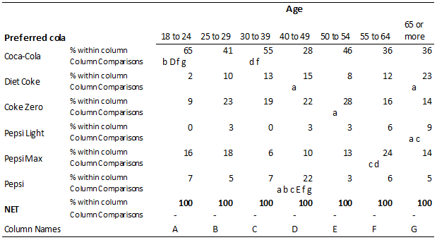
The table above shows column comparisons testing for differences in cola preference amongst different age groups. A total of 21 significance tests have been conducted in each row (i.e., this is the number of possible pairs of columns). The first row of the table shows that there are six significant differences between the age groups in terms of their preferences for Coca-Cola. The table below shows the 21 p-values.
| 18 to 24 | A | |||||||
| 25 to 29 | B | .0260 | ||||||
| 30 to 39 | C | .2895 | .1511 | |||||
| 40 to 49 | D | .0002 | .2062 | .0020 | ||||
| 50 to 54 | E | .0793 | .6424 | .3615 | .0763 | |||
| 55 to 64 | F | .0043 | .6295 | .0358 | .4118 | .3300 | ||
| 65 or more | G | .0250 | .7199 | .1178 | .5089 | .4516 | .9767 | |
| A | B | C | D | E | F | G | ||
| 18 to 24 | 25 to 29 | 30 to 39 | 40 to 49 | 50 to 54 | 55 to 64 | 65 or more |
If testing at the 0.05 level of significance we would anticipate that when conducting 21 tests we have a non-trivial chance of getting a false discovery by chance alone. If it is the case that, in reality, there is no real difference between the true proportions, we would expect that with 21 tests at the 0.05 level we will get an average of 21 × 0.05 = 1.05 to be significant (i.e., 0, 1, 2, with decreasing probabilities of higher results).
The cause of the problem relates to the underlying meaning of the p-value. The p-value is defined as the probability that we would get a result as a big or bigger than the one observed if, in fact, there is no difference in the population (see Formal Hypothesis Testing). When we conduct a single significance test, our error rate (i.e., the probability of false discoveries) is just the p-value itself[note 1]. For example, if we have a p-value of 0.05 and we conclude it is significant the probability of a false discovery is, by definition, 0.05. However, the more tests we do, the greater the probability of false discoveries.
If we have two unrelated tests and both have a p-value of 0.05 and are concluded to be significant, we can compute the following probabilities:
- The probability that both results are false discoveries is 0.05 × 0.05 = 0.0025.
- The probability that one but not both of the results is significant is 0.05 × 0.95 + 0.95 × 0.05 = 0.095.
- The probability that neither of the results is a false discovery is 0.95 × 0.95 = 0.9025.
The sum of these first two probabilities, 0.0975, is the probability of getting 1 or more false discoveries if there is no actual differences. This is often known as the familywise error rate. If we do 21 independent tests at the 0.05 level, our probability of one or more false discoveries jumps to 1 — (1 — 0.05)21 ≈ 0.58. Thus, we have a better than even chance of obtaining a false discovery on every single row of a table such as the table shown above when doing column comparisons. The consequence of this is dire, as it implies that many and perhaps most statistically significant results may be false discoveries.
Various corrections to statistical testing procedures have been developed to minimize the number of false discoveries that occur when conducting multiple tests. The next section provides an overview of some of the multiple comparison corrections. The section after that lists different strategies for applying multiple comparison corrections to tables.
Multiple comparison corrections
Many corrections have been developed for multiple comparisons. The simplest and most widely known is the Bonferroni correction. Its simplicity is not a virtue and it is doubtful that the Bonferroni correction should be widely used in survey research.
Numerous improvements over the Bonferroni correction were developed in the middle of the 20th century. These are briefly reviewed in the next sub-section. Then, the False Discovery Rate, which dominates most modern research in this field, is described.
Bonferroni correction
As computed above, if we are conducting 21 independent tests and the truth is that the null hypothesis is true in all instances, when we test at the 0.05 level we have a 58% chance of 1 or more false discoveries. Using the same maths, but in reverse, if we wish to reduce the probability of making one or more false discoveries to 0.05 we should conduct each test at the [math]displaystyle{ 1-sqrt[21]{1 — 0.05}=0.00244 }[/math] level of significance.
The Bonferroni inequality is an approximate formula for doing this computation. The approximation is that [math]displaystyle{ 1-sqrt[k]{1-alpha} approx alpha/21 }[/math], and thus in our example, [math]displaystyle{ alpha/m = 0.05/21 = 0.00238 approx 0.00244 }[/math] (where [math]displaystyle{ alpha }[/math] is the significance level and [math]displaystyle{ m }[/math] is the number of tests).
The Bonferroni correction involves testing for significance using the significance level for each test of [math]displaystyle{ alpha/k }[/math]. Thus, returning to the table of p-values above, only two of the pairs have p-values less than or equal to the new cut-off of 0.00244, A-D and C-D, so these are concluded to be statistically significant.
As mentioned above, while the Bonferroni correction is simple and it certainly reduces the number of false discoveries, it is in many ways a poor correction.
Poor power
The Bonferroni correction results in a large reduction in the power of statistical tests. That is, because the cut-off value is reduced, it becomes substantially more difficult for any result to be concluded as being statistically significant, irrespective of whether it is true or not. To use the jargon, the Bonferroni correction results in a loss of power (i.e., the ability of the test to reject the null hypothesis when it is false declines). In a sense this is a necessary outcome of any multiple comparison correction as the proportion of false discoveries and the power of a test are two sides of the same coin. However, the problem with the Bonferroni correction is that it loses more power than any of the alternative multiple comparison corrections and this loss of power does not confer any other benefits (other than simplicity).
Counterintuitive results
Consider a situation where 10 tests have been conducted and each has a p-value of 0.01. Using the Bonferroni correction with a significance level of 0.05 results in all the ten tests being concluded as not being statistically significant. That is, the corrected cut-off for concluding statistical significance is 0.05 / 10 = 0.005 and 0.01 > 0.005.
When we do lots of tests we are guaranteed to make a few false discoveries if the truth is that there there are no real differences in the data (i.e., the null hypothesis is always true). The whole logic is one of relatively rare events — that is the false discoveries — inevitably occurring because we conduct so many tests. However, in the example of 10 tests where all have a p-value of 0.01 it seems highly unlikely that the null hypothesis can be true in all of these instances and yet this is precisely the conclusion that the Bonferroni correction leads to.
In practice, this problem does occur regularly. The false discovery rate, which is described later, is a substantial improvement over the Bonferroni correction and it is discussed below.
Traditional non-Bonferroni corrections
Numerous alternatives have been developed to the Bonferroni correction. Popular corrections include Fisher LSD, Tukey’s HSD, Duncan’s New Multiple Range Test and Newmann-Keulls (S-N-K).[1] The different corrections often lead to different results. With the example we have been discussing, Tukey’s HSD finds two comparisons significant, Newmann-Keulls (S-N-K) finds three, Duncan’s New Multiple Range Test finds four and and Fisher LSD finds six.
In general, these tests have superior power to the Bonferroni correction. However, most of these tests are only applicable when comparing one numeric variables between multiple independent groups. That is, while the Bonferroni correction assumes independence, it can still be applied when this assumption is not met. However, most of the traditional alternatives to the Bonferroni correction can only be computed when comparing one numeric variable between multiple groups. Although these traditional corrections can be modified to deal with comparisons of proportions, they generally cannot be modified to deal with multiple response data and they are thus inapplicable to much of survey analysis. Furthermore, these corrections can generally not be employed with cell comparisons. Consequently, these alternatives tend only to be used in quite specialized areas (e.g., psychology experiments and sensory research), as in the more general survey analysis there is little merit in adopting a multiple comparison procedure that can only be used some of the time.
False Discovery Rate correction
The Bonferroni correction, which uses a cut-off of α / m where α is the significance level and m is the number of tests, is computed using the assumption that that the null hypothesis is correct for all the tests. However, when the assumption is not met, the correction itself is incorrect.
The table below orders all of the p-values from lowest to highest. The most smallest p-value is 0.0002 and this is below the Bonferroni cut-off of 0.00244 so we conclude it is significant. The next smallest p-value of 0.0020 is also below the Bonferroni cut-off so it is also concluded to be significant. However, the third smallest p-value of 0.0043 is greater than the cut-off which means that when applying the Bonferroni correction we conclude that it is not significant. However, this is faulty logic. If we believe that the first two smallest p-values indicate that the differences being tested are real, we have already come to a conclusion that the underlying assumption of the Bonferroni correction is false (i.e., we have determined that we do not believe that the null hypothesis is true for the first two corrections). Consequently, when computing the correction we should at the least ignore the first two comparisons, resulting in a revised cut-off of 0.05/(21-2)=0.00263.
| Comparison | p-Value | Test number | Cut-offs | Naïve significance | FDR significance | Bonferroni significance |
|---|---|---|---|---|---|---|
| D-A | .0002 | 1 | .0024 | D-A | D-A | D-A |
| D-C | .0020 | 2 | .0048 | D-C | D-C | D-C |
| F-A | .0043 | 3 | .0071 | F-A | F-A | |
| G-A | .0250 | 4 | .0095 | G-A | ||
| B-A | .0260 | 5 | .0119 | B-A | ||
| F-C | .0358 | 6 | .0143 | F-C | ||
| E-D | .0763 | 7 | .0167 | |||
| E-A | .0793 | 8 | .0190 | |||
| G-C | .1178 | 9 | .0214 | |||
| C-B | .1511 | 10 | .0238 | |||
| D-B | .2062 | 11 | .0262 | |||
| C-A | .2895 | 12 | .0286 | |||
| F-E | .3300 | 13 | .0310 | |||
| E-C | .3615 | 14 | .0333 | |||
| F-D | .4118 | 15 | .0357 | |||
| G-E | .4516 | 16 | .0381 | |||
| G-D | .5089 | 17 | .0405 | |||
| F-B | .6295 | 18 | .0429 | |||
| E-B | .6424 | 19 | .0452 | |||
| G-B | .7199 | 20 | .0476 | |||
| G-F | .9767 | 21 | .0500 |
While the cut-off of 0.00263 is more appropriate than the cut-off of 0.00244, it is still not quite right. The problem is that in assuming that we have 21 — 2 = 19 comparisons where the null hypothesis is true, we are forgetting that we have already determined that 2 of the tests are significant. This information is pertinent in that we if we believe that at least 2/21 tests are significant then it is overly pessimistic to base a computation of the cut-off rate for the rest of the tests on the assumption that the null hypothesis is true in all instances.
It has been shown that an appropriate cut-off procedure, which is referred to as the False Discovery Rate correction is:[2]
- Rank order all the tests from by smallest to largest p-value.
- Apply a cut-off based on the position in the rank-order. In particular, where i denotes the position in the rank order, starting from 1 for the most significant result and going through to m for the least significant result, the cut-off should be at least as high as α × i / m.
- Use largest significant cut-off as the overall cut-off. That is, it is possible using this formula that the smallest p-value will be bigger than the cut-off but that some other p-value be less than or equal to the cut-off (because the cut-off is different for each p-value. In such a situation, the cut-off that is largest is then re-applied to all the p-values.
Thus, returning to our third smallest p-value of 0.0043, the appropriate cut-off becomes 0.05 × 3 / 21 = 0.007143 and thus the third comparison is concluded to be significant. Thus, the false discovery rate leads to more results being significant than with the Bonferroni correction.
Some technical details about False Discovery Rate corrections
- The False Discovery Rate correction is a much newer technique than the traditional multiple comparison correction techniques. In the biological sciences, which is at the heart of much of modern statistical testing, the FDR is the default approach to dealing with multiple comparisons. However, the method is stull relatively unknown in survey research. Nevertheless, there is good reason to believe that the false discovery rate is superior. Where in survey research we have no real way of knowing when we are correct, in the biological sciences they often reproduce their studies and the popularity of the false discovery rate approach is presumably attributable to its accuracy.
- The above description states that «the cut-off should be at least as high» as that suggested by the formula. It is possible to calculate a more accurate cut-off,[3] but this entails a considerable increase in complexity. The more accurate cut-offs are always greater than or equal to the one described above and thus have greater power.
- In the discussion of the Bonferroni correction it was noted that with 10 tests each with a p-value of 0.04, none are significant when testing at the 0.05 level. By contrast, with the False Discovery Rate correction, all are found to be significant (i.e., the False Discovery Rate correction is substantially more powerful than the Bonferroni correction).
- The False Discovery Rate correction has a slightly different object to the Bonferroni correction (and other traditional corrections). While the Bonferroni correction is focused on trying to reduce the familywise error rate, the False Discovery Rate correction seeks to try and reduce the rate of false discoveries. That is, when the cut-off of α × i / m is used it is guaranteed that the at most α × 100% of discoveries will be false. Thus, α is really the false discovery rate rather than the familywise error rate and for this reason it is sometimes referred to as q to avoid confusion. There are no hard and fast rules about what value of q is appropriate. It is not unknown to have it as high as 0.20 (i.e., meaning that 20% of results will be “false”).
- Although the False Discovery Rate correction is computed under an assumption that the tests are independent, the approach still works much better than either traditional testing or the Bonferroni correction when this assumption is not met, such as when conducting pairwise comparisons[4]
Strategies for applying multiple comparison corrections to tables
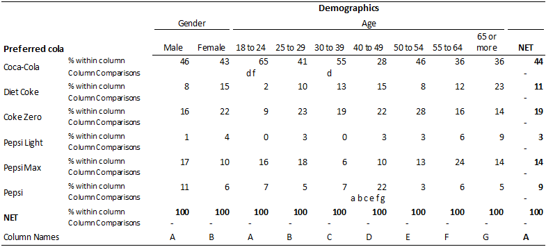
The table below shows a crosstab involving a banner that has both age and gender. When applying multiple comparison corrections a decision needs to be made about which tests to use in any correction. For example, if investigating the difference in preference for Coca-Cola between people aged 18 to 24 and those aged 55 to 64 we can:
- Ignore all the other tests and employ the Formal Hypothesis Testing approach.
- Only take into account the other 20 comparisons of preference for Coca-Cola by age (as done in the above examples). Thus, 21 comparisons are taken into account.
- Take into account all the comparisons involving Coca-Cola preference on this table. As there is also a comparison between gender, this involves 22 different comparisons.
- Take into account all the comparisons involving cola preferences and age. As there are six colas and 21 comparisons within each this results in 126 comparisons.
- Take into account all the comparisons on the table (i.e., 132 comparisons).
- Take into account all the comparisons involving Coca-Cola preference in the entire study (e.g., comparisons by income, occupation, etc.).
- Take into account all the comparison of all the cola preferences in the entire study.
- Take into account all the comparisons of any type in the study.
Looking at the Bonferroni correction (due to its simplicity), we can see that a problem we face is that the more comparisons we make the smaller the cut-off level becomes. When we employ Formal Hypothesis Testing the cut-off is 0.05, when we take into account 21 comparisons the cut-off drops to 0.05 / 21 = 0.0024. When we take into account 132 comparisons the cut-off drops to 0.0004. With most studies, such small cut-off results can lead to few and sometimes no results being marked as significant and thus the cure to the problem of false discoveries become possibly worse than the problem itself.
The False Discovery Rate correction is considerably better in this situation because the cut-off is computed from the data and if the data contains lots of small p-values the false discovery rate can identify lots of significant results, even in very large numbers of comparisons (e.g., millions). Nevertheless, a pragmatic problem is that if wanting to take into account comparisons that occur across multiple tables then one needs to work out which tables will be created. This can be practical in situations where there is a finite number of comparisons of interest (e.g., if wanting to compare everything by demographics). However, it is quite unusual that the number of potential comparisons of interest is fixed and, as a result, it is highly unusual in survey research to attempt to perform corrections for multiple comparisons across multiple tables (unless testing for significance of the entire table, rather than of results within a table).
The other traditional multiple comparison corrections, such as Tukey HSD and Fisher LSD, can only be computed in the situation involving comparisons within a row for independent sub-groups (i.e., the situation used in the worked examples above involving 21 comparisons).
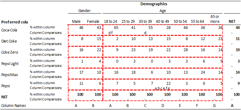
Within survey research, the convention with column comparisons is to perform comparisons within rows and within sets of related categories, as shown on the table below. Where a multiple comparison correction is made for cell comparisons the convention is to apply the comparison to the whole table (although this is a weak convention, as corrects for cell comparisons are not common). The difference between these two approaches is likely because the cell comparisons are generally more powerful and thus applying the correction to the whole table is not as dire.
Software comparisons
Most programs used for creating tables do not provide multiple comparison corrections. Most statistical programs do provide multiple comparisons corrections, however, they are generally not available as a part of any routines used for creating tables. For example, R contains a large number of possible corrections (including multiple variants of the False Discovery Rate correction), but they need to be programmed one-by-one if used for crosstabs and there is no straightforward way of displaying their results (i.e., R does not create tables with either Cell Comparisons or Column Comparisons).
| Package | Support for multiple comparison corrections |
|---|---|
| Excel | No support. |
| Q | Can perform False Discovery Rate correction on all tables using Cell Comparisons and/or Column Comparisons and can apply a number of the traditional corrections (Bonferroni, Tukey HSD, etc.) on Column Comparisons of means and proportions. Corrections can be conducted for the whole table, or, within row and related categories (Within row and span to use the Q terminology). |
| SPSS | Supports most traditional corrections as a part of its various analysis of variance tools (e.g., Analyze : Compare Means : One-Way ANOVA : Post Hoc), but does not use False Discovery Rate corrections. Bonferroni corrections can be placed on tables involving Column Comparisons in the Custom Tables module. |
| Wincross | For crosstabs involving means can perform a number of the traditional multiple comparison corrections. |
Also known as
- Post hoc testing
- Multiple comparison procedures
- Correction for data dredging
- Correction for data snooping
- Correction for data mining (this usage is very old-fashioned and predates the use of data mining techniques).
- Multiple hypothesis testing
See also
- Formal Hypothesis Testing
- The Role of Statistical Tests in Survey Analysis
- Statistical Tests on Tables
- Why Significance Test Results Change When Columns Are Added Or Removed
Notes
Template:Reflist
References
Template:Reflist
Cite error: <ref> tags exist for a group named «note», but no corresponding <references group="note"/> tag was found
- ↑ Hochberg, Y. and A. C. Tamhane (1987). Multiple Comparison Procedures. New York, Wiley.
- ↑ Benjamini, Y. and Y. Hochberg (1995). «Controlling the False Discovery Rate: A Practical and Powerful Approach to Multiple Testings.» Journal of the Royal Statistical Society — Series B 57(1): 289-300.
- ↑ Story, J. D. (2002). «A direct approach to false discovery rates.» Journal of the Royal Statistical Society, Series B (Methodological) 64 (3): 479–498 64(3): 479-498.
- ↑ Yoav Benjamini (2010): Discovering the false discovery rate, J. R. Statist. Soc. B (2010), 72, Part 4, pp. 405–416.