- numpy.polyfit(x, y, deg, rcond=None, full=False, w=None, cov=False)[source]#
-
Least squares polynomial fit.
Note
This forms part of the old polynomial API. Since version 1.4, the
new polynomial API defined innumpy.polynomialis preferred.
A summary of the differences can be found in the
transition guide.Fit a polynomial
p(x) = p[0] * x**deg + ... + p[deg]of degree deg
to points (x, y). Returns a vector of coefficients p that minimises
the squared error in the order deg, deg-1, … 0.The
Polynomial.fitclass
method is recommended for new code as it is more stable numerically. See
the documentation of the method for more information.- Parameters:
-
- xarray_like, shape (M,)
-
x-coordinates of the M sample points
(x[i], y[i]). - yarray_like, shape (M,) or (M, K)
-
y-coordinates of the sample points. Several data sets of sample
points sharing the same x-coordinates can be fitted at once by
passing in a 2D-array that contains one dataset per column. - degint
-
Degree of the fitting polynomial
- rcondfloat, optional
-
Relative condition number of the fit. Singular values smaller than
this relative to the largest singular value will be ignored. The
default value is len(x)*eps, where eps is the relative precision of
the float type, about 2e-16 in most cases. - fullbool, optional
-
Switch determining nature of return value. When it is False (the
default) just the coefficients are returned, when True diagnostic
information from the singular value decomposition is also returned. - warray_like, shape (M,), optional
-
Weights. If not None, the weight
w[i]applies to the unsquared
residualy[i] - y_hat[i]atx[i]. Ideally the weights are
chosen so that the errors of the productsw[i]*y[i]all have the
same variance. When using inverse-variance weighting, use
w[i] = 1/sigma(y[i]). The default value is None. - covbool or str, optional
-
If given and not False, return not just the estimate but also its
covariance matrix. By default, the covariance are scaled by
chi2/dof, where dof = M — (deg + 1), i.e., the weights are presumed
to be unreliable except in a relative sense and everything is scaled
such that the reduced chi2 is unity. This scaling is omitted if
cov='unscaled', as is relevant for the case that the weights are
w = 1/sigma, with sigma known to be a reliable estimate of the
uncertainty.
- Returns:
-
- pndarray, shape (deg + 1,) or (deg + 1, K)
-
Polynomial coefficients, highest power first. If y was 2-D, the
coefficients for k-th data set are inp[:,k]. - residuals, rank, singular_values, rcond
-
These values are only returned if
full == True-
residuals – sum of squared residuals of the least squares fit
-
- rank – the effective rank of the scaled Vandermonde
-
coefficient matrix
-
- singular_values – singular values of the scaled Vandermonde
-
coefficient matrix
-
rcond – value of rcond.
For more details, see
numpy.linalg.lstsq. -
- Vndarray, shape (M,M) or (M,M,K)
-
Present only if
full == Falseandcov == True. The covariance
matrix of the polynomial coefficient estimates. The diagonal of
this matrix are the variance estimates for each coefficient. If y
is a 2-D array, then the covariance matrix for the k-th data set
are inV[:,:,k]
- Warns:
-
- RankWarning
-
The rank of the coefficient matrix in the least-squares fit is
deficient. The warning is only raised iffull == False.The warnings can be turned off by
>>> import warnings
>>> warnings.simplefilter('ignore', np.RankWarning)
Notes
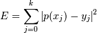
The solution minimizes the squared error
[E = sum_{j=0}^k |p(x_j) — y_j|^2]
in the equations:
x[0]**n * p[0] + ... + x[0] * p[n-1] + p[n] = y[0]
x[1]**n * p[0] + ... + x[1] * p[n-1] + p[n] = y[1]
...
x[k]**n * p[0] + ... + x[k] * p[n-1] + p[n] = y[k]
The coefficient matrix of the coefficients p is a Vandermonde matrix.
polyfitissues aRankWarningwhen the least-squares fit is badly
conditioned. This implies that the best fit is not well-defined due
to numerical error. The results may be improved by lowering the polynomial
degree or by replacing x by x — x.mean(). The rcond parameter
can also be set to a value smaller than its default, but the resulting
fit may be spurious: including contributions from the small singular
values can add numerical noise to the result.Note that fitting polynomial coefficients is inherently badly conditioned
when the degree of the polynomial is large or the interval of sample points
is badly centered. The quality of the fit should always be checked in these
cases. When polynomial fits are not satisfactory, splines may be a good
alternative.References
Examples
>>> import warnings
>>> x = np.array([0.0, 1.0, 2.0, 3.0,  4.0,  5.0])
>>> y = np.array([0.0, 0.8, 0.9, 0.1, -0.8, -1.0])
>>> z = np.polyfit(x, y, 3)
>>> z
array([ 0.08703704, -0.81349206,  1.69312169, -0.03968254]) # may vary
It is convenient to use
poly1dobjects for dealing with polynomials:>>> p = np.poly1d(z) >>> p(0.5) 0.6143849206349179 # may vary >>> p(3.5) -0.34732142857143039 # may vary >>> p(10) 22.579365079365115 # may vary
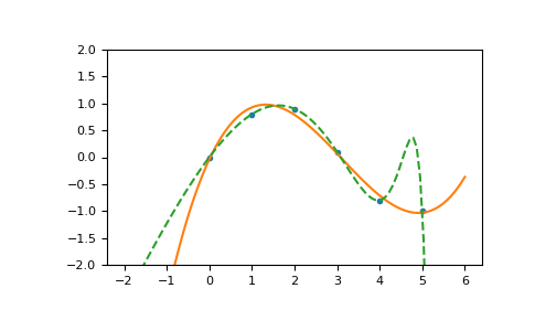
High-order polynomials may oscillate wildly:
>>> with warnings.catch_warnings(): ... warnings.simplefilter('ignore', np.RankWarning) ... p30 = np.poly1d(np.polyfit(x, y, 30)) ... >>> p30(4) -0.80000000000000204 # may vary >>> p30(5) -0.99999999999999445 # may vary >>> p30(4.5) -0.10547061179440398 # may vary
Illustration:
>>> import matplotlib.pyplot as plt >>> xp = np.linspace(-2, 6, 100) >>> _ = plt.plot(x, y, '.', xp, p(xp), '-', xp, p30(xp), '--') >>> plt.ylim(-2,2) (-2, 2) >>> plt.show()

- numpy.polyfit(x, y, deg, rcond=None, full=False, w=None, cov=False)[source]
-
Least squares polynomial fit.
Fit a polynomial p(x) = p[0] * x**deg + … + p[deg] of degree deg
to points (x, y). Returns a vector of coefficients p that minimises
the squared error.Parameters: x : array_like, shape (M,)
x-coordinates of the M sample points (x[i], y[i]).
y : array_like, shape (M,) or (M, K)
y-coordinates of the sample points. Several data sets of sample
points sharing the same x-coordinates can be fitted at once by
passing in a 2D-array that contains one dataset per column.deg : int
Degree of the fitting polynomial
rcond : float, optional
Relative condition number of the fit. Singular values smaller than
this relative to the largest singular value will be ignored. The
default value is len(x)*eps, where eps is the relative precision of
the float type, about 2e-16 in most cases.full : bool, optional
Switch determining nature of return value. When it is False (the
default) just the coefficients are returned, when True diagnostic
information from the singular value decomposition is also returned.w : array_like, shape (M,), optional
weights to apply to the y-coordinates of the sample points.
cov : bool, optional
Return the estimate and the covariance matrix of the estimate
If full is True, then cov is not returned.Returns: p : ndarray, shape (M,) or (M, K)
Polynomial coefficients, highest power first. If y was 2-D, the
coefficients for k-th data set are in p[:,k].residuals, rank, singular_values, rcond :
Present only if full = True. Residuals of the least-squares fit,
the effective rank of the scaled Vandermonde coefficient matrix,
its singular values, and the specified value of rcond. For more
details, see linalg.lstsq.V : ndarray, shape (M,M) or (M,M,K)
Present only if full = False and cov`=True. The covariance
matrix of the polynomial coefficient estimates. The diagonal of
this matrix are the variance estimates for each coefficient. If y
is a 2-D array, then the covariance matrix for the `k-th data set
are in V[:,:,k]Warns: RankWarning
The rank of the coefficient matrix in the least-squares fit is
deficient. The warning is only raised if full = False.The warnings can be turned off by
>>> import warnings >>> warnings.simplefilter('ignore', np.RankWarning)
See also
- polyval
- Computes polynomial values.
- linalg.lstsq
- Computes a least-squares fit.
- scipy.interpolate.UnivariateSpline
- Computes spline fits.
Notes
The solution minimizes the squared error
in the equations:
x[0]**n * p[0] + ... + x[0] * p[n-1] + p[n] = y[0] x[1]**n * p[0] + ... + x[1] * p[n-1] + p[n] = y[1] ... x[k]**n * p[0] + ... + x[k] * p[n-1] + p[n] = y[k]
The coefficient matrix of the coefficients p is a Vandermonde matrix.
polyfit issues a RankWarning when the least-squares fit is badly
conditioned. This implies that the best fit is not well-defined due
to numerical error. The results may be improved by lowering the polynomial
degree or by replacing x by x — x.mean(). The rcond parameter
can also be set to a value smaller than its default, but the resulting
fit may be spurious: including contributions from the small singular
values can add numerical noise to the result.Note that fitting polynomial coefficients is inherently badly conditioned
when the degree of the polynomial is large or the interval of sample points
is badly centered. The quality of the fit should always be checked in these
cases. When polynomial fits are not satisfactory, splines may be a good
alternative.References
[R58] Wikipedia, “Curve fitting”,
http://en.wikipedia.org/wiki/Curve_fitting[R59] Wikipedia, “Polynomial interpolation”,
http://en.wikipedia.org/wiki/Polynomial_interpolationExamples
>>> x = np.array([0.0, 1.0, 2.0, 3.0, 4.0, 5.0]) >>> y = np.array([0.0, 0.8, 0.9, 0.1, -0.8, -1.0]) >>> z = np.polyfit(x, y, 3) >>> z array([ 0.08703704, -0.81349206, 1.69312169, -0.03968254])
It is convenient to use poly1d objects for dealing with polynomials:
>>> p = np.poly1d(z) >>> p(0.5) 0.6143849206349179 >>> p(3.5) -0.34732142857143039 >>> p(10) 22.579365079365115
High-order polynomials may oscillate wildly:
>>> p30 = np.poly1d(np.polyfit(x, y, 30)) /... RankWarning: Polyfit may be poorly conditioned... >>> p30(4) -0.80000000000000204 >>> p30(5) -0.99999999999999445 >>> p30(4.5) -0.10547061179440398
Illustration:
>>> import matplotlib.pyplot as plt >>> xp = np.linspace(-2, 6, 100) >>> _ = plt.plot(x, y, '.', xp, p(xp), '-', xp, p30(xp), '--') >>> plt.ylim(-2,2) (-2, 2) >>> plt.show()
(Source code)
Introduction to np.polyfit() function
The np.polyfit() is a NumPy library function that fits a polynomial to a set of data points. Given two arrays x and y representing the x-coordinates and y-coordinates of the data points, the np.polyfit() function returns the coefficients of the polynomial that best fits the data.
The np.polyfit() method takes a few parameters and returns a vector of coefficients p that minimizes the squared error in the order deg, deg-1, … 0.
It least squares the polynomial fit. It fits a polynomial p(X) of degree deg to points (X, Y).
The Polynomial.fit class method is recommended for new code as it is numerically stable. It is a fit polynomial p(x) = p[0] * x**deg + … + p[deg] of degree deg to points (x, y).
Syntax
numpy.polyfit (X, Y, deg, rcond=None, full=False, w=None, cov=False)Parameters
This function takes at most seven parameters:
X: array_like,
Suppose it has a shape of size (M). In a sample of M examples, it represents the x-coordinates (X[i],Y[i])
Y: array_like,
it has a shape of (M,) or (M, K). It represents the y-coordinates (X[i], Y[i]) of sample points.
deg: int,
It should be an integer value and specify the degree to which the polynomial should be made fit.
rcond: float. It is an optional parameter.
It describes the relative condition number of the fit. Those singular values smaller than this relative to the largest singular value will be ignored.
full: It’s an optional parameter of the Boolean type
It acts as a switch and helps determine the nature of the return value. For example, when the value is set to false (the default), only the coefficients are returned; when the value is set to true diagnostic info from the singular value decomposition is additionally returned.
w: array_like, shape(M,), optional
These are weights that are applied to the Y-coordinates of the sample points. For gaussian uncertainties, we should use 1/sigma (not 1/sigma**2).
cov: bool or str, optional parameter
If provided and is not set to False, it returns the estimate and its covariance matrix. The covariance is, by default, scaled by chi**2/sqrt(N-dof), i.e., the weights are presumed to be unreliable except in a relative sense, and everything is scaled such that the reduced chi2 is unity.
If cov=’ unscaled’, then the scaling is omitted as it is relevant because the weights are 1/sigma**2, with sigma being known to be a reliable estimate of the uncertainty.
Return Value
It returns a ndarray, shape (deg+1,) or (deg+1, K)
This method returns an n-dimensional array of shape (deg+1) when the Y array has the shape of (M,) or in case the Y array has the shape of (M, K), then an n-dimensional array of shape (deg+1, K) is returned.
If Y is 2-Dimensional, the coefficients for the Kth dataset are in p [:, K].
Programming Example:
Program to show the working of numpy.polyfit() method.
# importing the numpy module
import numpy as np
# Creating a dataset
x = np.arange(-5, 5)
print("X values in the dataset are:n", x)
y = np.arange(-30, 30, 6)
print("Y values in the dataset are:n", y)
# calculating value of coefficients in case of linear polynomial
z = np.polyfit(x, y, 1)
print("ncoefficient value in case of linear polynomial:n", z)
# calculating value of coefficient in case of quadratic polynomial
z1 = np.polyfit(x, y, 2)
print("ncoefficient value in case of quadratic polynomial:n", z1)
# calculating value of coefficient in case of cubic polynomial
z2 = np.polyfit(x, y, 3)
print("ncoefficient value in case of cubic polynomial:n", z2)Output
X values in the dataset are:
[-5 -4 -3 -2 -1 0 1 2 3 4]
Y values in the dataset are:
[-30 -24 -18 -12 -6 0 6 12 18 24]
coefficient value in case of linear polynomial:
[6.00000000e+00 4.62412528e-16]
coefficient value in case of quadratic polynomial:
[ 1.36058326e-16 6.00000000e+00 -2.24693342e-15]
coefficient value in case of cubic polynomial:
[ 1.10709805e-16 0.00000000e+00 6.00000000e+00 -8.42600032e-16]Explanation
In the above program, we have created a dataset (x,y) using the np.arange() method, and the various data points are displayed.
If we want to fit these data points into a polynomial of various degrees like linear (having degree 1), which is y=mx+c, we need to have two constant-coefficient values for m c, which is calculated using the numpy.polyfit() function.
Similarly, in the case of a quadratic equation (having degree 2), which is of the form y=ax**2+bx+c, we need to have three constant-coefficient values for a, b, and s calculated using the numpy.polyfit() function.
The same is the case with a cubic polynomial of the form y=ax**3+bx**2+cx+d; we need to have four constant-coefficient values for a, b, c, and d calculated using the numpy.polyfit() function.
Using np.polyfit() method to implement linear regression
import numpy as np
import matplotlib.pyplot as plt
x = np.arange(0, 30, 3)
print("X points are: n", x)
y = x**2
print("Y points are: n", y)
plt.scatter(x, y)
plt.xlabel("X-values")
plt.ylabel("Y-values")
plt.plot(x, y)
p = np.polyfit(x, y, 2) # Last argument is degree of polynomial
print("Coeeficient values:n", p)
predict = np.poly1d(p)
x_test = 15
print("nGiven x_test value is: ", x_test)
y_pred = predict(x_test)
print("nPredicted value of y_pred for given x_test is: ", y_pred)Output
X points are:
[ 0 3 6 9 12 15 18 21 24 27]
Y points are:
[ 0 9 36 81 144 225 324 441 576 729]
Coeeficient values:
[ 1.00000000e+00 -2.02043144e-14 2.31687975e-13]
Given x_test value is: 15
Predicted value of y_pred for given x_test is: 225.00000000000009
Explanation
In the program polyfit2.py, we have created a dataset (x, y) method, and the various data points are displayed and plotted onto a graph.
Now, we want to fit this dataset into a polynomial of degree 2, a quadratic polynomial of the form y=ax**2+bx+c, so we need to calculate three constant-coefficient values for a, b, and c, which is calculated using the numpy.polyfit() function.
These coefficient values signify the best fit that our polynomial function can have concerning the data points. We can predict our y values based on some given x_test values, which are also shown.
That’s it.
Conclusion
The np.polyfit() is a built-in numpy library method that fits our data inside a polynomial function.
See also
np.inner
np.correlate
Linear regression is the first step to learn data science. So even if you are new in this field, you have to understand these concepts because these algorithms are mostly used by data science researchers. These algorithms are also easy to understand to start the machine learning journey.
In this tutorial, we are going to see the numpy(polyfit) regression model.
The function numpy.polyfit () finds the best fit line by minimizing the sum of squared error. This method accepts three parameters:
- x – input data
- y- output data
- Polynomial degree value (integer)
So, let’s start the step-by-step process to use the method polyfit.
Step 1: Import all the required library and packages to run this program.
<img alt=»» data-lazy- data-lazy-src=»https://kirelos.com/wp-content/uploads/2021/08/echo/NumPy-Polyfit-1.png» data-lazy- height=»168″ src=»data:image/svg xml,” width=”1230″>
Line 91: We import the NumPy and matplotlib library. The polyfit automatically comes under the NumPy, so no need to import. The matplotlib is used to plot the data and matplotlib inline is used to draw the graph inside of the jupyter notebook itself.
import numpy as np
import matplotlib.pyplot as plt
%matplotlib inline
Step 2: Now, our next step is to create dataset (x and y).
<img alt=»» data-lazy- data-lazy-src=»https://kirelos.com/wp-content/uploads/2021/08/echo/NumPy-Polyfit-2.png» data-lazy- height=»165″ src=»data:image/svg xml,” width=”1204″>
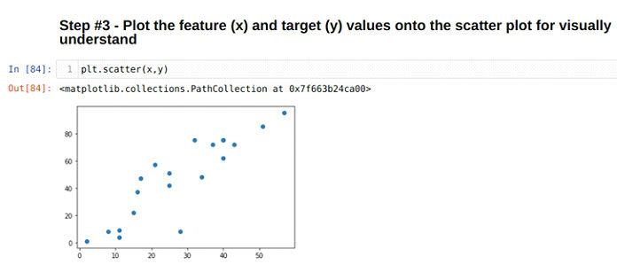
Line 83: We randomly generate the x and y data.
x= [28, 8, 11, 37, 15, 25, 51, 11, 32, 34, 43, 2, 40, 16, 40, 25, 40, 17, 21, 57]
y= [8, 8, 9, 72, 22, 51, 85, 4, 75, 48, 72, 1, 62, 37, 75, 42, 75, 47, 57, 95]
Step 3: We are just going to plot the feature (x) and target (y) on the graph as shown below:
<img alt=»» data-lazy- data-lazy-src=»https://kirelos.com/wp-content/uploads/2021/08/echo/NumPy-Polyfit-3.png» data-lazy- height=»470″ src=»data:image/svg xml,” width=”1209″>
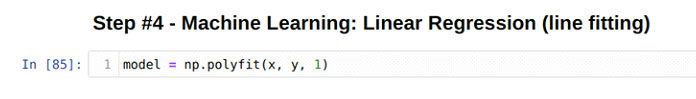
Step 4: In this step, we are going to fit the line on the data x and y.
<img alt=»» data-lazy- data-lazy-src=»https://kirelos.com/wp-content/uploads/2021/08/echo/NumPy-Polyfit-4.png» data-lazy- height=»130″ src=»data:image/svg xml,” width=”1215″>
This step is very easy because we are going to use the concept of the polyfit method. The polyfit method directly comes with the Numpy as shown above. This method accepts three parameters:
- x – input data
- y- output data
- Polynomial degree value (integer)
In this program, we are using the polynomial degree value 1, which says that it is a first-degree polynomial. But we can also use it for second and third-degree polynomial.
1 model = np.polyfit(x, y, 1)
When we press the enter, the polyfit calculates the linear regression model and store to the right-hand side variable model.
Logic Behind the Fitting Line
So, we can see that just hitting the enter key and we got out linear regression model. So now we are thinking that, what actually works behind of this method and how they fitting the line.
The method which works behind of the polyfit method is called ordinary least square method. Some people called this with the short name OLS. It is commonly used by the users to fit the line. The reason behind is it’s very easy to use and also gives accuracy above 90%.
Let’s see how OLS perform:
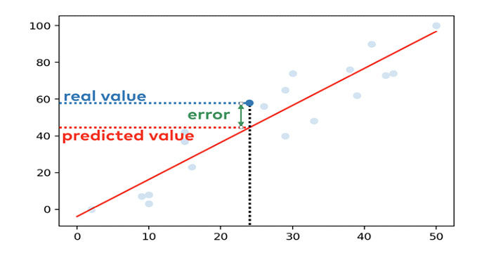
First, we need to know about error. The error calculates through the difference between the x and y data.
For example, we fit a line on the regression model which looks like below:
<img alt=»» data-lazy- data-lazy-src=»https://kirelos.com/wp-content/uploads/2021/08/echo/NumPy-Polyfit-5.png» data-lazy- height=»720″ src=»data:image/svg xml,” width=”1080″>
The blue dots are the data points and the red line which we fit on the data points using the polyfit method.
Let’s assume x = 24 and y = 58
When we fit the line, the line calculates the value of y = 44.3. The difference between the actual and calculated value is the error for the specific data point.
<img alt=»» data-lazy- data-lazy-src=»https://kirelos.com/wp-content/uploads/2021/08/echo/NumPy-Polyfit-6.png» data-lazy- height=»782″ src=»data:image/svg xml,” width=”1402″>
So, the OLS (ordinary least square) method calculates the fit using the below steps:
1. Calculates the error between the fitted model and the data points.
<img alt=»» data-lazy- data-lazy-src=»https://kirelos.com/wp-content/uploads/2021/08/echo/NumPy-Polyfit-7.png» data-lazy- height=»800″ src=»data:image/svg xml,” width=”1210″>
2. Then we square each of the data points error.
3. Sum all the square data points error.
4. Finally, identify the line where this sum of the squared error is minimum.
So, the polyfit uses the above methods to fit the line.
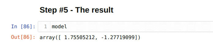
Step 5: Model
We have done our machine learning coding part. Now, we can check the values of x and y which are stored in the model variables. To check the x and y value, we have to print the model as shown below:
<img alt=»» data-lazy- data-lazy-src=»https://kirelos.com/wp-content/uploads/2021/08/echo/NumPy-Polyfit-8.png» data-lazy- height=»123″ src=»data:image/svg xml,” width=”1211″>
Finally, we got an outline equation:
y = 1.75505212 * x – 1.27719099
By using this linear equation, we can get the value of y.
The above linear equation can also be solved using the ploy1d() method like below:
predict = np.poly1d(model)
x_value = 20
predict(x_value)
<img alt=»» data-lazy- data-lazy-src=»https://kirelos.com/wp-content/uploads/2021/08/echo/NumPy-Polyfit-9.png» data-lazy- height=»112″ src=»data:image/svg xml,” width=”1204″>
We got the result 33.82385131766588.
We also got the same result from the manual calculation:
y = 1.75505212 * 20 – 1.27719099
y = 33.82385131766588
So, both the above results show that our model fits the line correctly.
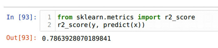
Step 6: Accuracy of the model
We can also check the accuracy of the model, either it gives correct results or not. The accuracy of the model can be calculated from the R-squared (R2). The value of the R-squared (R2) is between 0 and 1. The result close to 1 will show that model accuracy is high. So, let’s check for the above model accuracy. We will import another library, sklearn, as shown below:
from sklearn.metrics import r2_score
r2_score(y, predict(x))
<img alt=»» data-lazy- data-lazy-src=»https://kirelos.com/wp-content/uploads/2021/08/echo/NumPy-Polyfit-10.png» data-lazy- height=»110″ src=»data:image/svg xml,” width=”1206″>
The result shows that it is close to 1, so its accuracy is high.
Step 7: Plotting the model
The plotting is the method to see the model fitted line on the data points visually. It gives clear image of the model.
<img alt=»» data-lazy- data-lazy-src=»https://kirelos.com/wp-content/uploads/2021/08/echo/NumPy-Polyfit-11.png» data-lazy- height=»488″ src=»data:image/svg xml,” width=”1210″>
x_axis = range(0, 60)
y_axis = predict(x_axis)
plt.scatter(x, y)
plt.plot(x_axis, y_axis, c = ‘g’)
A quick explanation for the above plot method is given below:
Line 1: It is the range which we want to display on the plot. In our code, we are using the range value from 0 to 60.
Line 2: All the range values from 0 to 60 will be calculated.
Line 3: We pass those x and y original datasets into the scatter method.
Line 4: We finally plot our graph, and the green line is the fit line as shown in the above graph.
Conclusion
In this article, we have learned the linear regression model which is the start of the journey of machine learning. There is a number of regression models that are explained in another article. Here, we have a clean dataset because that was a dummy, but in real-life projects, you might get a dirty dataset and you have to do feature engineering on that to clean the dataset to use in the model. If you do not fully understand this tutorial, even that helps you to learn another regression model easily.
The line regression model is the most common algorithm used by data science. You must have ideas about the regression model if you want to have your career in this field. So, keep in touch and soon we will be back with a new data science article.
Least squares polynomial fit.
Note
This forms part of the old polynomial API. Since version 1.4, the new polynomial API defined in numpy.polynomial is preferred. A summary of the differences can be found in the transition guide.
Fit a polynomial p(x) = p[0] * x**deg + ... + p[deg] of degree deg to points (x, y). Returns a vector of coefficients p that minimises the squared error in the order deg, deg-1, … 0.
The Polynomial.fit class method is recommended for new code as it is more stable numerically. See the documentation of the method for more information.
- Parameters
-
-
xarray_like, shape (M,) -
x-coordinates of the M sample points
(x[i], y[i]). -
yarray_like, shape (M,) or (M, K) -
y-coordinates of the sample points. Several data sets of sample points sharing the same x-coordinates can be fitted at once by passing in a 2D-array that contains one dataset per column.
-
degint -
Degree of the fitting polynomial
-
rcondfloat, optional -
Relative condition number of the fit. Singular values smaller than this relative to the largest singular value will be ignored. The default value is len(x)*eps, where eps is the relative precision of the float type, about 2e-16 in most cases.
-
fullbool, optional -
Switch determining nature of return value. When it is False (the default) just the coefficients are returned, when True diagnostic information from the singular value decomposition is also returned.
-
warray_like, shape (M,), optional -
Weights to apply to the y-coordinates of the sample points. For gaussian uncertainties, use 1/sigma (not 1/sigma**2).
-
covbool or str, optional -
If given and not
False, return not just the estimate but also its covariance matrix. By default, the covariance are scaled by chi2/dof, where dof = M — (deg + 1), i.e., the weights are presumed to be unreliable except in a relative sense and everything is scaled such that the reduced chi2 is unity. This scaling is omitted ifcov='unscaled', as is relevant for the case that the weights are 1/sigma**2, with sigma known to be a reliable estimate of the uncertainty.
-
- Returns
-
-
pndarray, shape (deg + 1,) or (deg + 1, K) -
Polynomial coefficients, highest power first. If
ywas 2-D, the coefficients fork-th data set are inp[:,k]. - residuals, rank, singular_values, rcond
-
Present only if
full= True. Residuals is sum of squared residuals of the least-squares fit, the effective rank of the scaled Vandermonde coefficient matrix, its singular values, and the specified value ofrcond. For more details, seelinalg.lstsq. -
Vndarray, shape (M,M) or (M,M,K) -
Present only if
full= False andcov`=True. The covariance matrix of the polynomial coefficient estimates. The diagonal of this matrix are the variance estimates for each coefficient. If y is a 2-D array, then the covariance matrix for the `k-th data set are inV[:,:,k]
-
- Warns
-
- RankWarning
-
The rank of the coefficient matrix in the least-squares fit is deficient. The warning is only raised if
full= False.The warnings can be turned off by
>>> import warnings >>> warnings.simplefilter('ignore', np.RankWarning)
Notes
The solution minimizes the squared error
in the equations:
x[0]**n * p[0] + ... + x[0] * p[n-1] + p[n] = y[0] x[1]**n * p[0] + ... + x[1] * p[n-1] + p[n] = y[1] ... x[k]**n * p[0] + ... + x[k] * p[n-1] + p[n] = y[k]
The coefficient matrix of the coefficients p is a Vandermonde matrix.
polyfit issues a RankWarning when the least-squares fit is badly conditioned. This implies that the best fit is not well-defined due to numerical error. The results may be improved by lowering the polynomial degree or by replacing x by x — x.mean(). The rcond parameter can also be set to a value smaller than its default, but the resulting fit may be spurious: including contributions from the small singular values can add numerical noise to the result.
Note that fitting polynomial coefficients is inherently badly conditioned when the degree of the polynomial is large or the interval of sample points is badly centered. The quality of the fit should always be checked in these cases. When polynomial fits are not satisfactory, splines may be a good alternative.
References
-
1 -
Wikipedia, “Curve fitting”, https://en.wikipedia.org/wiki/Curve_fitting
-
2 -
Wikipedia, “Polynomial interpolation”, https://en.wikipedia.org/wiki/Polynomial_interpolation
Examples
>>> import warnings >>> x = np.array([0.0, 1.0, 2.0, 3.0, 4.0, 5.0]) >>> y = np.array([0.0, 0.8, 0.9, 0.1, -0.8, -1.0]) >>> z = np.polyfit(x, y, 3) >>> z array([ 0.08703704, -0.81349206, 1.69312169, -0.03968254]) # may vary
It is convenient to use poly1d objects for dealing with polynomials:
>>> p = np.poly1d(z)
>>> p(0.5)
0.6143849206349179 # may vary
>>> p(3.5)
-0.34732142857143039 # may vary
>>> p(10)
22.579365079365115 # may vary
High-order polynomials may oscillate wildly:
>>> with warnings.catch_warnings():
...     warnings.simplefilter('ignore', np.RankWarning)
...     p30 = np.poly1d(np.polyfit(x, y, 30))
...
>>> p30(4)
-0.80000000000000204 # may vary
>>> p30(5)
-0.99999999999999445 # may vary
>>> p30(4.5)
-0.10547061179440398 # may vary
Illustration:
>>> import matplotlib.pyplot as plt
>>> xp = np.linspace(-2, 6, 100)
>>> _ = plt.plot(x, y, '.', xp, p(xp), '-', xp, p30(xp), '--')
>>> plt.ylim(-2,2)
(-2, 2)
>>> plt.show()
Наименее квадраты полиномиальные.
Note
Это часть старого полиномиального API. Начиная с версии 1.4, новый полиномиальный API, определенный в numpy.polynomial , является предпочтительным. Сводку различий можно найти в руководстве по переходу .
Подгонка многочлена p(x) = p[0] * x**deg + ... + p[deg] степени deg к точкам (x, y) . Возвращает вектор коэффициентов p , который минимизирует квадрат ошибки в порядке deg , deg-1 , … 0 .
Для нового кода рекомендуется использовать метод класса Polynomial.fit , поскольку он более стабилен численно. Дополнительную информацию см. В документации по методу.
- Parameters
-
- x подобный массиву, форма (M,)
-
x-координаты M точек выборки
(x[i], y[i]). - y array_like, shape (M,) или (M, K)
-
y-координаты точек выборки.Несколько наборов данных точек выборки,имеющих одни и те же x-координаты,могут быть подогнаны сразу путем пропускания в 2D-массиве,содержащем один набор данных на колонку.
- degint
-
Степень установки полинома
- rcondfloat, optional
-
Относительное состояние номер подгонки.Сингулярные значения меньше этого относительно наибольшего сингулярного значения будут проигнорированы.Значением по умолчанию является len(x)*eps,где eps-относительная точность типа float,в большинстве случаев около 2e-16.
- fullbool, optional
-
Переключатель определения характера возвращаемого значения.При False (по умолчанию)возвращаются только коэффициенты,когда также возвращается True диагностическая информация из сингулярного разложения значений.
- w array_like, форма (M,), необязательно
-
Веса. Если не None, вес
w[i]применяется к неквадратичному остаткуy[i] - y_hat[i]вx[i]. В идеале веса выбираются так, чтобы ошибки произведенийw[i]*y[i]имели одинаковую дисперсию. При использовании взвешивания обратной дисперсии используйтеw[i] = 1/sigma(y[i]). Значение по умолчанию — Нет. - cov bool или str, необязательно
-
Если задано, а не
False, вернуть не только оценку, но и ее ковариационную матрицу. По умолчанию ковариация масштабируется как chi2/dof, где dof = M — (deg + 1), т. е. предполагается, что веса ненадежны, кроме как в относительном смысле, и все масштабируется таким образом, что приведенный chi2 равен единице. Это масштабирование опускается, еслиcov='unscaled', что важно для случая, когда веса равны w = 1/сигма, причем сигма, как известно, является надежной оценкой неопределенности.
- Returns
-
- p ndarray, shape (deg + 1,) или (deg + 1, K)
-
Коэффициенты полинома, сначала наивысшая степень. Если
yбыло 2-D, коэффициенты дляk-го набора данных находятся вp[:,k]. - остатки,ранг,сингулярные_значения,rcond
-
Эти значения возвращаются, только если
full == True- остатки-сумма квадратов остатков при подгонке по методу наименьших квадратов
-
- ранг-эффективный ранг масштабированного Вандермонда
-
coefficient matrix
-
- singular_values-сингулярные значения масштаба Вандермонда
-
coefficient matrix
- rcond – значение
rcond.
Для получения дополнительных сведений см.
numpy.linalg.lstsq. - V ndarray, форма (M, M) или (M, M, K)
-
Присутствует, только если
full == Falseиcov == True. Ковариационная матрица оценок полиномиальных коэффициентов. Диагональ этой матрицы представляет собой оценки дисперсии для каждого коэффициента. Если y представляет собой двумерный массив, то ковариационная матрица дляk-го набора данных находится вV[:,:,k]
- Warns
-
- RankWarning
-
Ранг матрицы коэффициентов в подгонке по методу наименьших квадратов недостаточен. Предупреждение возникает только в том случае, если
full == False.Предупреждения могут быть отключены
>>> import warnings
>>> warnings.simplefilter('ignore', np.RankWarning)
Notes
Решение минимизирует квадратную ошибку
[E = sum_{j=0}^k |p(x_j) — y_j|^2]
в уравнениях:
x[0]**n * p[0] + ... + x[0] * p[n-1] + p[n] = y[0]
x[1]**n * p[0] + ... + x[1] * p[n-1] + p[n] = y[1]
...
x[k]**n * p[0] + ... + x[k] * p[n-1] + p[n] = y[k]
Матрица коэффициентов коэффициентов p является матрицей Вандермонда.
polyfit выдает RankWarning , когда соответствие методом наименьших квадратов плохо обусловлено. Это означает, что наилучшее соответствие не определено четко из-за числовой ошибки. Результаты можно улучшить, понизив степень полинома или заменив x на x — x .mean (). Параметр rcond также может быть установлен на значение, меньшее, чем значение по умолчанию, но полученное соответствие может быть ложным: включение небольших сингулярных значений может добавить числовой шум к результату.
Обратите внимание,что подгоночные полиномиальные коэффициенты по своей природе плохо обусловлены,когда степень полинома велика или интервал точек выборки плохо отцентрирован.В этих случаях всегда следует проверять качество подгонки.В случае неудовлетворительной посадки полинома хорошей альтернативой могут быть сплайны.
References
- 1
-
Википедия, «Подбор кривой», https://en.wikipedia.org/wiki/Curve_fitting
- 2
-
Википедия, «Полиномиальная интерполяция», https://en.wikipedia.org/wiki/Polynomial_interpolation
Examples
>>> import warnings >>> x = np.array([0.0, 1.0, 2.0, 3.0, 4.0, 5.0]) >>> y = np.array([0.0, 0.8, 0.9, 0.1, -0.8, -1.0]) >>> z = np.polyfit(x, y, 3) >>> z array([ 0.08703704, -0.81349206, 1.69312169, -0.03968254]) # may vary
Для работы с полиномами удобно использовать объекты poly1d :
>>> p = np.poly1d(z) >>> p(0.5) 0.6143849206349179 # may vary >>> p(3.5) -0.34732142857143039 # may vary >>> p(10) 22.579365079365115 # may vary
Полиномы высокого порядка могут дико колебаться:
>>> with warnings.catch_warnings(): ... warnings.simplefilter('ignore', np.RankWarning) ... p30 = np.poly1d(np.polyfit(x, y, 30)) ... >>> p30(4) -0.80000000000000204 # may vary >>> p30(5) -0.99999999999999445 # may vary >>> p30(4.5) -0.10547061179440398 # may vary
Illustration:
>>> import matplotlib.pyplot as plt
>>> xp = np.linspace(-2, 6, 100)
>>> _ = plt.plot(x, y, '.', xp, p(xp), '-', xp, p30(xp), '--')
>>> plt.ylim(-2,2)
(-2, 2)
>>> plt.show()
На чтение 6 мин Просмотров 2.1к. Опубликовано 19.08.2021
Линейная регрессия — это первый шаг к изучению науки о данных. Поэтому, даже если вы новичок в этой области, вы должны понимать эти концепции, потому что эти алгоритмы в основном используются исследователями в области науки о данных. Эти алгоритмы также легко понять, чтобы начать путешествие по машинному обучению.
В этом руководстве мы увидим модель регрессии numpy (polyfit).
Функция numpy.polyfit () находит наиболее подходящую линию, минимизируя сумму квадратов ошибок. Этот метод принимает три параметра:
- x — входные данные
- y- выходные данные
- Значение степени полинома (целое число)
Итак, приступим к пошаговому процессу использования метода polyfit.
Шаг 1. Импортируйте всю необходимую библиотеку и пакеты для запуска этой программы.

Строка 91: мы импортируем библиотеки NumPy и matplotlib. Polyfit автоматически попадает под NumPy, поэтому нет необходимости импортировать. Matplotlib используется для построения данных, а matplotlib inline используется для рисования графика внутри самого ноутбука jupyter.
import numpy as np
import matplotlib.pyplot as plt
%matplotlib inline
Шаг 2: Теперь наш следующий шаг — создать набор данных (x и y).

Строка 83: мы произвольно генерируем данные x и y.
x= [28, 8, 11, 37, 15, 25, 51, 11, 32, 34, 43, 2, 40, 16, 40, 25, 40, 17, 21, 57]
y= [8, 8, 9, 72, 22, 51, 85, 4, 75, 48, 72, 1, 62, 37, 75, 42, 75, 47, 57, 95]
Шаг 3: Мы просто собираемся нанести объект (x) и цель (y) на график, как показано ниже:
Шаг 4: На этом шаге мы собираемся подогнать линию к данным x и y.
Этот шаг очень прост, потому что мы собираемся использовать концепцию метода полифита. Метод polyfit напрямую поставляется с Numpy, как показано выше. Этот метод принимает три параметра:
- x — входные данные
- y- выходные данные
- Значение степени полинома (целое число)
В этой программе мы используем значение степени полинома 1, что означает, что это многочлен первой степени. Но мы также можем использовать его для полиномов второй и третьей степени.
1 model = np.polyfit(x, y, 1)
Когда мы нажимаем Enter, полифит вычисляет модель линейной регрессии и сохраняет в правой части модель переменных.
Логика за подходящей линией
Итак, мы видим, что просто нажав клавишу ввода, мы получили модель линейной регрессии. Итак, теперь мы думаем о том, что на самом деле работает за этим методом и как они подходят к линии.
Метод, который работает позади метода полифита, называется обычным методом наименьших квадратов. Некоторые назвали это коротким названием OLS. Пользователи обычно используют его, чтобы подогнать под линию. Причина в том, что он очень прост в использовании, а также дает точность выше 90%.
Посмотрим, как работает OLS:
Во-первых, нам нужно знать об ошибке. Ошибка вычисляется через разницу между данными x и y.
Например, мы помещаем линию в регрессионную модель, которая выглядит следующим образом:
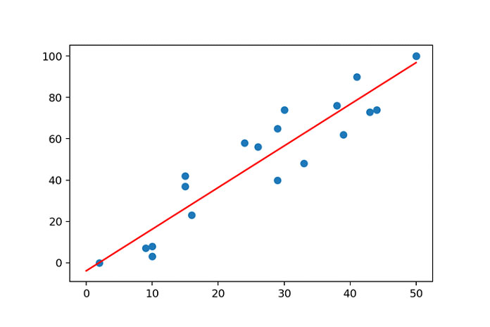
Синие точки — это точки данных, а красная линия, которую мы помещаем в точки данных, используя метод polyfit.
Предположим, что x = 24 и y = 58.
Когда мы подбираем линию, она вычисляет значение y = 44,3. Разница между фактическим и расчетным значением — это ошибка для конкретной точки данных.
Итак, метод наименьших квадратов (OLS) вычисляет аппроксимацию, используя следующие шаги:
- Вычисляет ошибку между подобранной моделью и точками данных.

- Затем мы возводим в квадрат каждую ошибку точек данных.
- Просуммируйте все ошибки квадратных точек данных.
- Наконец, определите линию, в которой сумма квадратов ошибок минимальна.

Итак, полифит использует вышеуказанные методы для подгонки линии.
Шаг 5: Модель
Мы закончили кодирование машинного обучения. Теперь мы можем проверить значения x и y, которые хранятся в переменных модели. Чтобы проверить значения x и y, мы должны распечатать модель, как показано ниже:
Наконец, мы получили контурное уравнение:
у = 1,75505212 * х — 1,27719099
Используя это линейное уравнение, мы можем получить значение y.
Вышеупомянутое линейное уравнение также можно решить с помощью метода ploy1d (), как показано ниже:
predict = np.poly1d(model)
x_value = 20
predict(x_value)

Получили результат 33.82385131766588.
Тот же результат мы получили и от ручного расчета:
у = 1,75505212 * 20 — 1,27719099
у = 33,82385131766588
Итак, оба приведенных выше результата показывают, что наша модель правильно подходит для этой линии.
Шаг 6: точность модели
Мы также можем проверить точность модели, дает ли она правильные результаты или нет. Точность модели можно рассчитать с помощью R-квадрата (R2). Значение R-квадрата (R2) находится между 0 и 1. Результат, близкий к 1, показывает, что точность модели высока. Итак, проверим точность приведенной выше модели. Мы импортируем другую библиотеку, sklearn, как показано ниже:
from sklearn.metrics import r2_score
r2_score(y, predict(x))
Результат показывает, что он близок к 1, поэтому его точность высока.
Шаг 7: Построение модели
Построение графика — это метод визуального просмотра линии, подобранной модели, на точках данных. Это дает четкое изображение модели.

x_axis = range(, 60)
y_axis = predict(x_axis)
plt.scatter(x, y)
plt.plot(x_axis, y_axis, c = ‘g’)
Краткое объяснение вышеуказанного метода построения графиков приведено ниже:
1 строка : это диапазон, который мы хотим отобразить на графике. В нашем коде мы используем значение диапазона от 0 до 60.
2 строка: будут вычислены все значения диапазона от 0 до 60.
3 строка: мы передаем исходные наборы данных x и y в метод разброса.
4 строка: Мы, наконец, строим наш график, и зеленая линия является подходящей линией, как показано на приведенном выше графике.
Заключение
В этой статье мы узнали о модели линейной регрессии, которая является началом пути машинного обучения. Существует ряд регрессионных моделей, которые описаны в другой статье. Здесь у нас есть чистый набор данных, потому что он был фиктивным, но в реальных проектах вы можете получить грязный набор данных, и вам нужно будет выполнить проектирование функций для этого, чтобы очистить набор данных для использования в модели. Если вы не полностью понимаете этот учебник, даже он поможет вам легко изучить другую модель регрессии.
Модель линейной регрессии — наиболее распространенный алгоритм, используемый в науке о данных. У вас должно быть представление о регрессионной модели, если вы хотите сделать карьеру в этой области.