В первой части были рассмотрены: структура, топология, функции активации и обучающее множество. В этой части попробую объяснить как происходит обучение сверточной нейронной сети.
Обучение сверточной нейронной сети
На начальном этапе нейронная сеть является необученной (ненастроенной). В общем смысле под обучением понимают последовательное предъявление образа на вход нейросети, из обучающего набора, затем полученный ответ сравнивается с желаемым выходом, в нашем случае это 1 – образ представляет лицо, минус 1 – образ представляет фон (не лицо), полученная разница между ожидаемым ответом и полученным является результат функции ошибки (дельта ошибки). Затем эту дельту ошибки необходимо распространить на все связанные нейроны сети.
Таким образом обучение нейронной сети сводится к минимизации функции ошибки, путем корректировки весовых коэффициентов синаптических связей между нейронами. Под функцией ошибки понимается разность между полученным ответом и желаемым. Например, на вход был подан образ лица, предположим, что выход нейросети был 0.73, а желаемый результат 1 (т.к. образ лица), получим, что ошибка сети является разницей, то есть 0.27. Затем веса выходного слоя нейронов корректируются в соответствии с ошибкой. Для нейронов выходного слоя известны их фактические и желаемые значения выходов. Поэтому настройка весов связей для таких нейронов является относительно простой. Однако для нейронов предыдущих слоев настройка не столь очевидна. Долгое время не было известно алгоритма распространения ошибки по скрытым слоям.
Алгоритм обратного распространения ошибки
Для обучения описанной нейронной сети был использован алгоритм обратного распространения ошибки (backpropagation). Этот метод обучения многослойной нейронной сети называется обобщенным дельта-правилом. Метод был предложен в 1986 г. Румельхартом, Макклеландом и Вильямсом. Это ознаменовало возрождение интереса к нейронным сетям, который стал угасать в начале 70-х годов. Данный алгоритм является первым и основным практически применимым для обучения многослойных нейронных сетей.
Для выходного слоя корректировка весов интуитивна понятна, но для скрытых слоев долгое время не было известно алгоритма. Веса скрытого нейрона должны изменяться прямо пропорционально ошибке тех нейронов, с которыми данный нейрон связан. Вот почему обратное распространение этих ошибок через сеть позволяет корректно настраивать веса связей между всеми слоями. В этом случае величина функции ошибки уменьшается и сеть обучается.
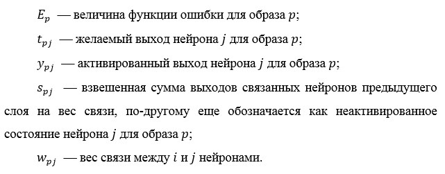
Основные соотношения метода обратного распространения ошибки получены при следующих обозначениях:
Величина ошибки определяется по формуле 2.8 среднеквадратичная ошибка:

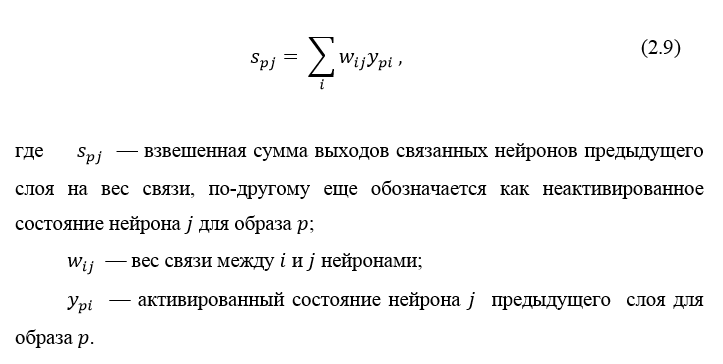
Неактивированное состояние каждого нейрона j для образа p записывается в виде взвешенной суммы по формуле 2.9:
Выход каждого нейрона j является значением активационной функции
 , которая переводит нейрон в активированное состояние. В качестве функции активации может использоваться любая непрерывно дифференцируемая монотонная функция. Активированное состояние нейрона вычисляется по формуле 2.10:

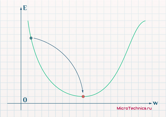
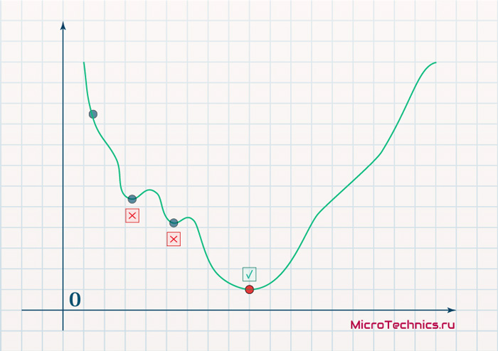
В качестве метода минимизации ошибки используется метод градиентного спуска, суть этого метода сводится к поиску минимума (или максимума) функции за счет движения вдоль вектора градиента. Для поиска минимума движение должно быть осуществляться в направлении антиградиента. Метод градиентного спуска в соответствии с рисунком 2.7.

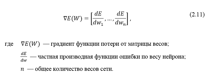
Градиент функции потери представляет из себя вектор частных производных, вычисляющийся по формуле 2.11:
Производную функции ошибки по конкретному образу можно записать по правилу цепочки, формула 2.12:

Ошибка нейрона  обычно записывается в виде символа δ (дельта). Для выходного слоя ошибка определена в явном виде, если взять производную от формулы 2.8, то получим t минус y, то есть разницу между желаемым и полученным выходом. Но как рассчитать ошибку для скрытых слоев? Для решения этой задачи, как раз и был придуман алгоритм обратного распространения ошибки. Суть его заключается в последовательном вычислении ошибок скрытых слоев с помощью значений ошибки выходного слоя, т.е. значения ошибки распространяются по сети в обратном направлении от выхода к входу.
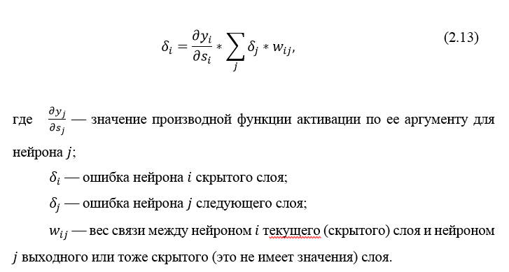
Ошибка δ для скрытого слоя рассчитывается по формуле 2.13:
Алгоритм распространения ошибки сводится к следующим этапам:
- прямое распространение сигнала по сети, вычисления состояния нейронов;
- вычисление значения ошибки δ для выходного слоя;
- обратное распространение: последовательно от конца к началу для всех скрытых слоев вычисляем δ по формуле 2.13;
- обновление весов сети на вычисленную ранее δ ошибки.
Алгоритм обратного распространения ошибки в многослойном персептроне продемонстрирован ниже:
До этого момента были рассмотрены случаи распространения ошибки по слоям персептрона, то есть по выходному и скрытому, но помимо них, в сверточной нейросети имеются подвыборочный и сверточный.
Расчет ошибки на подвыборочном слое
Расчет ошибки на подвыборочном слое представляется в нескольких вариантах. Первый случай, когда подвыборочный слой находится перед полносвязным, тогда он имеет нейроны и связи такого же типа, как в полносвязном слое, соответственно вычисление δ ошибки ничем не отличается от вычисления δ скрытого слоя. Второй случай, когда подвыборочный слой находится перед сверточным, вычисление δ происходит путем обратной свертки. Для понимания обратно свертки, необходимо сперва понять обычную свертку и то, что скользящее окно по карте признаков (во время прямого распространения сигнала) можно интерпретировать, как обычный скрытый слой со связями между нейронами, но главное отличие — это то, что эти связи разделяемы, то есть одна связь с конкретным значением веса может быть у нескольких пар нейронов, а не только одной. Интерпретация операции свертки в привычном многослойном виде в соответствии с рисунком 2.8.

Рисунок 2.8 — Интерпретация операции свертки в многослойный вид, где связи с одинаковым цветом имеют один и тот же вес. Синим цветом обозначена подвыборочная карта, разноцветным – синаптическое ядро, оранжевым – получившаяся свертка
Теперь, когда операция свертки представлена в привычном многослойном виде, можно интуитивно понять, что вычисление дельт происходит таким же образом, как и в скрытом слое полносвязной сети. Соответственно имея вычисленные ранее дельты сверточного слоя можно вычислить дельты подвыборочного, в соответствии с рисунком 2.9.
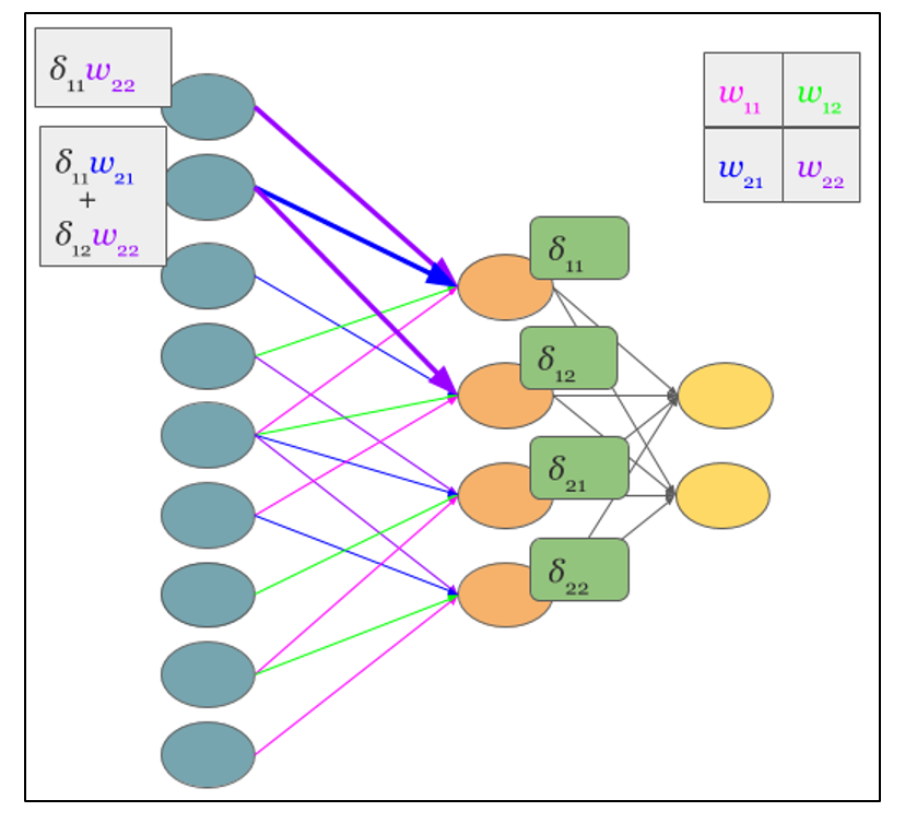
Рисунок 2.9 — Вычисление δ подвыборочного слоя за счет δ сверточного слоя и ядра
Обратная свертка – это тот же самый способ вычисления дельт, только немного хитрым способом, заключающийся в повороте ядра на 180 градусов и скользящем процессе сканирования сверточной карты дельт с измененными краевыми эффектами. Простыми словами, нам необходимо взять ядро сверточной карты (следующего за подвыборочным слоем) повернуть его на 180 градусов и сделать обычную свертку по вычисленным ранее дельтам сверточной карты, но так чтобы окно сканирования выходило за пределы карты. Результат операции обратной свертки в соответствии с рисунком 2.10, цикл прохода обратной свертки в соответствии с рисунком 2.11.

Рисунок 2.10 — Результат операции обратной свертки
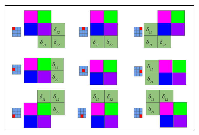
Рисунок 2.11 — Повернутое ядро на 180 градусов сканирует сверточную карту
Расчет ошибки на сверточном слое
Обычно впередиидущий слой после сверточного это подвыборочный, соответственно наша задача вычислить дельты текущего слоя (сверточного) за счет знаний о дельтах подвыборочного слоя. На самом деле дельта ошибка не вычисляется, а копируется. При прямом распространении сигнала нейроны подвыборочного слоя формировались за счет неперекрывающегося окна сканирования по сверточному слою, в процессе которого выбирались нейроны с максимальным значением, при обратном распространении, мы возвращаем дельту ошибки тому ранее выбранному максимальному нейрону, остальные же получают нулевую дельту ошибки.
Заключение
Представив операцию свертки в привычном многослойном виде (рисунок 2.8), можно интуитивно понять, что вычисление дельт происходит таким же образом, как и в скрытом слое полносвязной сети.
Источники
Алгоритм обратного распространения ошибки для сверточной нейронной сети
Обратное распространение ошибки в сверточных слоях
раз и два
Обратное распространение ошибки в персептроне
Еще можно почитать в РГБ диссертацию Макаренко: АЛГОРИТМЫ И ПРОГРАММНАЯ СИСТЕМА КЛАССИФИКАЦИИ
Рад снова всех приветствовать, и сегодня продолжим планомерно двигаться в выбранном направлении. Речь, конечно, о масштабном разборе искусственных нейронных сетей для решения широкого спектра задач. Продолжим ровно с того момента, на котором остановились в предыдущей части, и это означает, что героем данного поста будет ключевой процесс — обучение нейронных сетей.
Тема эта крайне важна, поскольку именно процесс обучения позволяет сети начать выполнять задачу, для которой она, собственно, и предназначена. То есть нейронная сеть функционирует не по какому-либо жестко заданному на этапе проектирования алгоритму, она совершенствуется в процессе анализа имеющихся данных. Этот процесс и называется обучением нейронной сети. Математически суть процесса обучения заключается в корректировке значений весов синапсов (связей между имеющимися нейронами). Изначально значения весов задаются случайно, затем производится обучение, результатом которого будут новые значения синаптических весов. Это все мы максимально подробно разберем как раз в этой статье.
На своем сайте я всегда придерживаюсь концепции, при которой теоретические выкладки по максимуму сопровождаются практическими примерами для максимальной наглядности. Так мы поступим и сейчас 👍
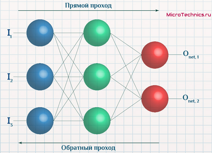
Итак, суть заключается в следующем. Пусть у нас есть простейшая нейронная сеть, которую мы хотим обучить (продолжаем рассматривать сети прямого распространения):

То есть на входы нейронов I1 и I2 мы подаем какие-либо числа, а на выходе сети получаем соответственно новое значение. При этом нам необходима некая выборка данных, включающая в себя значения входов и соответствующее им, правильное, значение на выходе:
| bold{I_1} | bold{I_2} | bold{O_{net}} |
|---|---|---|
| x_{11} | x_{12} | y_{1} |
| x_{21} | x_{22} | y_{2} |
| x_{31} | x_{32} | y_{3} |
| … | … | … |
| x_{N1} | x_{N2} | y_{N} |
Допустим, сеть выполняет суммирование значений на входе, тогда данный набор данных может быть таким:
| bold{I_1} | bold{I_2} | bold{O_{net}} |
|---|---|---|
| 1 | 4 | 5 |
| 2 | 7 | 9 |
| 3 | 5 | 8 |
| … | … | … |
| 1000 | 1500 | 2500 |
Эти значения и используются для обучения сети. Как именно — рассмотрим чуть ниже, пока сконцентрируемся на идее процесса в целом. Для того, чтобы иметь возможность тестировать работу сети в процессе обучения, исходную выборку данных делят на две части — обучающую и тестовую. Пусть имеется 1000 образцов, тогда можно 900 использовать для обучения, а оставшиеся 100 — для тестирования. Эти величины взяты исключительно ради наглядности и демонстрации логики выполнения операций, на практике все зависит от задачи, размер обучающей выборки может спокойно достигать и сотен тысяч образцов.
Итак, итог имеем следующий — обучающая выборка прогоняется через сеть, в результате чего происходит настройка значений синаптических весов. Один полный проход по всей выборке называется эпохой. И опять же, обучение нейронной сети — это процесс, требующий многократных экспериментов, анализа результатов и творческого подхода. Все перечисленные параметры (размер выборки, количество эпох обучения) могут иметь абсолютно разные значения для разных задач и сетей. Четкого правила тут просто нет, в этом и кроется дополнительный шарм и изящность )
Возвращаемся к разбору, и в результате прохода обучающей выборки через сеть мы получаем сеть с новыми значениями весов синапсов.
Далее мы через эту, уже обученную в той или иной степени, сеть прогоняем тестовую выборку, которая не участвовала в обучении. При этом сеть выдает нам выходные значения для каждого образца, которые мы сравниваем с теми верными значениями, которые имеем.
Анализируем нашу гипотетическую выборку:

Таким образом, для тестирования подаем на вход сети значения x_{(M+1)1}, x_{(M+1)2} и проверяем, чему равен выход, ожидаем очевидно значение y_{(M+1)}. Аналогично поступаем и для оставшихся тестовых образцов. После чего мы можем сделать вывод, успешно или нет работает сеть. Например, сеть дает правильный ответ для 90% тестовых данных, дальше уже встает вопрос — устраивает ли нас данная точность или процесс обучения необходимо повторить, либо провести заново, изменив какие-либо параметры сети.
В этом и заключается суть обучения нейронных сетей, теперь перейдем к деталям и конкретным действиям, которые необходимо осуществить для выполнения данного процесса. Двигаться снова будем поэтапно, чтобы сформировать максимально четкую и полную картину. Поэтому начнем с понятия градиентного спуска, который используется при обучении по методу обратного распространения ошибки. Обо всем этом далее…
Обучение нейронных сетей. Градиентный спуск.
Рассмотрев идею процесса обучения в целом, на данном этапе мы можем однозначно сформулировать текущую цель — необходимо определить математический алгоритм, который позволит рассчитать значения весовых коэффициентов таким образом, чтобы ошибка сети была минимальна. То есть грубо говоря нам необходима конкретная формула для вычисления:
Здесь Delta w_{ij} — величина, на которую необходимо изменить вес синапса, связывающего нейроны i и j нашей сети. Соответственно, зная это, необходимо на каждом этапе обучения производить корректировку весов связей между всеми элементами нейронной сети. Задача ясна, переходим к делу.
Пусть функция ошибки от веса имеет следующий вид:
Для удобства рассмотрим зависимость функции ошибки от одного конкретного веса:

В начальный момент мы находимся в некоторой точке кривой, а для минимизации ошибки попасть мы хотим в точку глобального минимума функции:
Нанесем на график вектора градиентов в разных точках. Длина векторов численно равна скорости роста функции в данной точке, что в свою очередь соответствует значению производной функции по данной точке. Исходя из этого, делаем вывод, что длина вектора градиента определяется крутизной функции в данной точке:
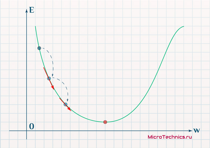
Вывод прост — величина градиента будет уменьшаться по мере приближения к минимуму функции. Это важный вывод, к которому мы еще вернемся. А тем временем разберемся с направлением вектора, для чего рассмотрим еще несколько возможных точек:
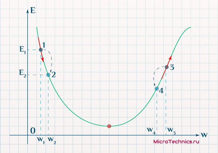
Находясь в точке 1, целью является перейти в точку 2, поскольку в ней значение ошибки меньше (E_2 < E_1), а глобальная задача по-прежнему заключается в ее минимизации. Для этого необходимо изменить величину w на некое значение Delta w (Delta w = w_2 — w_1 > 0). При всем при этом в точке 1 градиент отрицательный. Фиксируем данные факты и переходим к точке 3, предположим, что мы находимся именно в ней.
Тогда для уменьшения ошибки наш путь лежит в точку 4, а необходимое изменение значения: Delta w = w_4 — w_3 < 0. Градиент же в точке 3 положителен. Этот факт также фиксируем.
А теперь соберем воедино эту информацию в виде следующей иллюстрации:
| Переход | bold{Delta w} | Знак bold{Delta w} | Градиент |
|---|---|---|---|
| 1 rArr 2 | w_2 — w_1 | + | — |
| 3 rArr 4 | w_4 — w_3 | — | + |
Вывод напрашивается сам собой — величина, на которую необходимо изменить значение w, в любой точке противоположна по знаку градиенту. И, таким образом, представим эту самую величину в виде:
Delta w = -alpha cdot frac{dE}{dw}
Имеем в наличии:
- Delta w — величина, на которую необходимо изменить значение w.
- frac{dE}{dw} — градиент в этой точке.
- alpha — скорость обучения.
Собственно, логика метода градиентного спуска и заключается в данном математическом выражении, а именно в том, что для минимизации ошибки необходимо изменять w в направлении противоположном градиенту. В контексте нейронных сетей имеем искомый закон для корректировки весов синаптических связей (для синапса между нейронами i и j):
Delta w_{ij} = -alpha cdot frac{dE}{dw_{ij}}
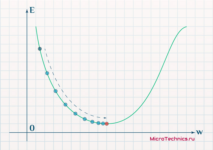
Более того, вспомним о важном свойстве, которое мы отдельно пометили. И заключается оно в том, что величина градиента будет уменьшаться по мере приближения к минимуму функции. Что это нам дает? А то, что в том случае, если наша текущая дислокация далека от места назначения, то величина, корректирующая вес связи, будет больше. А это обеспечит скорейшее приближение к цели. При приближении к целевому пункту, величина frac{dE}{dw_{ij}} будет уменьшаться, что поможет нам точнее попасть в нужную точку, а кроме того, не позволит нам ее проскочить. Визуализируем вышеописанное:
Скорость же обучения несет в себе следующий смысл. Она определяет величину каждого шага при поиске минимума ошибки. Слишком большое значение приводит к тому, что точка может «перепрыгнуть» через нужное значение и оказаться по другую сторону от цели:
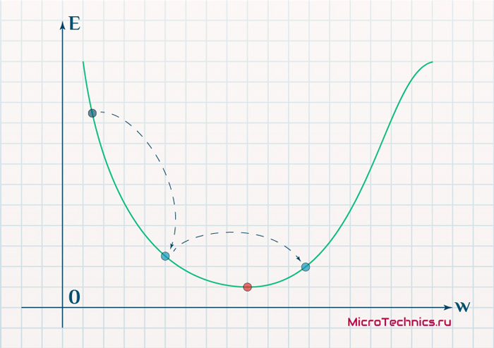
Если же величина будет мала, то это приведет к тому, что спуск будет осуществляться очень медленно, что также является нежелательным эффектом. Поэтому скорость обучения, как и многие другие параметры нейронной сети, является очень важной величиной, для которой нет единственно верного значения. Все снова зависит от конкретного случая и оптимальная величина определяется исключительно исходя из текущих условий.
И даже на этом еще не все, здесь присутствует один важный нюанс, который в большинстве статей опускается, либо вовсе не упоминается. Реальная зависимость может иметь совсем другой вид:
Из чего вытекает потенциальная возможность попадания в локальный минимум, вместо глобального, что является большой проблемой. Для предотвращения данного эффекта вводится понятие момента обучения и формула принимает следующий вид:
Delta w_{ij} = -alpha cdot frac{dE}{dw_{ij}} + gamma cdot Delta w_{ij}^{t - 1}
То есть добавляется второе слагаемое, которое представляет из себя произведение момента на величину корректировки веса на предыдущем шаге.
Итого, резюмируем продвижение к цели:
- Нашей задачей было найти закон, по которому необходимо изменять величину весов связей между нейронами.
- Наш результат — Delta w_{ij} = -alpha cdot frac{dE}{dw_{ij}} + gamma cdot Delta w_{ij}^{t — 1} — именно то, что и требовалось 👍
И опять же, полученный результат логичным образом перенаправляет нас на следующий этап, ставя вопросы — что из себя представляет функция ошибки, и как определить ее градиент.
Обучение нейронных сетей. Функция ошибки.
Начнем с того, что определимся с тем, что у нас в наличии, для этого вернемся к конкретной нейронной сети. Пусть вид ее таков:
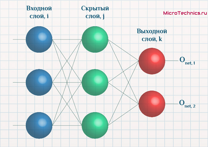
Интересует нас, в первую очередь, часть, относящаяся к нейронам выходного слоя. Подав на вход определенные значения, получаем значения на выходе сети: O_{net, 1} и O_{net, 2}. Кроме того, поскольку мы ведем речь о процессе обучения нейронной сети, то нам известны целевые значения: O_{correct, 1} и O_{correct, 2}. И именно этот набор данных на этом этапе является для нас исходным:
- Известно: O_{net, 1}, O_{net, 2}, O_{correct, 1} и O_{correct, 2}.
- Необходимо определить величины Delta w_{ij} для корректировки весов, для этого нужно вычислить градиенты (frac{dE}{dw_{ij}}) для каждого из синапсов.
Полдела сделано — задача четко сформулирована, начинаем деятельность по поиску решения.
В плане того, как определять ошибку, первым и самым очевидным вариантом кажется простая алгебраическая разность. Для каждого из выходных нейронов:
E_k = O_{correct, k} - O_{net, k}
Дополним пример числовыми значениями:
| Нейрон | bold{O_{net}} | bold{O_{correct}} | bold{E} |
|---|---|---|---|
| 1 | 0.9 | 0.5 | -0.4 |
| 2 | 0.2 | 0.6 | 0.4 |
Недостатком данного варианта является то, что в том случае, если мы попытаемся просуммировать ошибки нейронов, то получим:
E_{sum} = e_1 + e_2 = -0.4 + 0.4 = 0
Что не соответствует действительности (нулевая ошибка, говорит об идеальной работе нейронной сети, по факту оба нейрона дали неверный результат). Так что вариант с разностью откидываем за несостоятельностью.
Вторым, традиционно упоминаемым, методом вычисления ошибки является использование модуля разности:
E_k = | O_{correct, k} - O_{net, k} |
Тут в действие вступает уже проблема иного рода:
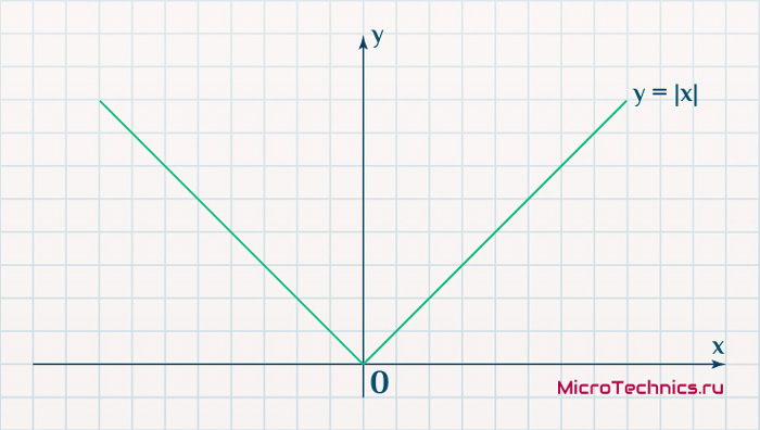
Функция, бесспорно, симпатична, но при приближении к минимуму ее градиент является постоянной величиной, скачкообразно меняясь при переходе через точку минимума. Это нас также не устраивает, поскольку, как мы обсуждали, концепция заключалась в том числе в том, чтобы по мере приближения к минимуму значение градиента уменьшалось.
В итоге хороший результат дает зависимость (для выходного нейрона под номером k):
E_k = (O_{correct, k} - O_{net, k})^2
Функция по многим своим свойствам идеально удовлетворяет нуждам обучения нейронной сети, так что выбор сделан, остановимся на ней. Хотя, как и во многих аспектах, качающихся нейронных сетей, данное решение не является единственно и неоспоримо верным. В каких-то случаях лучше себя могут проявить другие зависимости, возможно, что какой-то вариант даст большую точность, но неоправданно высокие затраты производительности при обучении. В общем, непаханное поле для экспериментов и исследований, это и привлекательно.
Краткий вывод промежуточного шага, на который мы вышли:
- Имеющееся: frac{dE}{dw_{jk}} = frac{d}{d w_{jk}}(O_{correct, k} — O_{net, k})^2.
- Искомое по-прежнему: Delta w_{jk}.
Несложные диффернциально-математические изыскания выводят на следующий результат:
frac{dE}{d w_{jk}} = -(O_{correct, k} - O_{net, k}) cdot f{Large{prime}}(sum_{j}w_{jk}O_j) cdot O_j
Здесь эти самые изыскания я все-таки решил не вставлять, дабы не перегружать статью, которая и так выходит объемной. Но в случае необходимости и интереса, отпишите в комментарии, я добавлю вычисления и закину их под спойлер, как вариант.
Освежим в памяти структуру сети:
Формулу можно упростить, сгруппировав отдельные ее части:
- (O_{correct, k} — O_{net, k}) cdot f{Large{prime}}(sum_{j}w_{jk}O_j) — ошибка нейрона k.
- O_j — тут все понятно, выходной сигнал нейрона j.
f{Large{prime}}(sum_{j}w_{jk}O_j) — значение производной функции активации. Причем, обратите внимание, что sum_{j}w_{jk}O_j — это не что иное, как сигнал на входе нейрона k (I_{k}). Тогда для расчета ошибки выходного нейрона: delta_k = (O_{correct, k} — O_{net, k}) cdot f{Large{prime}}(I_k).
Итог: frac{dE}{d w_{jk}} = -delta_k cdot O_j.
Одной из причин популярности сигмоидальной функции активности является то, что ее производная очень просто выражается через саму функцию:
f{'}(x) = f(x)medspace (1medspace-medspace f(x))
Данные алгебраические вычисления справедливы для корректировки весов между скрытым и выходным слоем, поскольку для расчета ошибки мы используем просто разность между целевым и полученным результатом, умноженную на производную.
Для других слоев будут незначительные изменения, касающиеся исключительно первого множителя в формуле:
frac{dE}{d w_{ij}} = -delta_j cdot O_i
Который примет следующий вид:
delta_j = (sum_{k}{}{delta_kmedspace w_{jk}}) cdot f{Large{prime}}(I_j)
То есть ошибка для элемента слоя j получается путем взвешенного суммирования ошибок, «приходящих» к нему от нейронов следующего слоя и умножения на производную функции активации. В результате:
frac{dE}{d w_{ij}} = -(sum_{k}{}{delta_kmedspace w_{jk}}) cdot f{Large{prime}}(I_j) cdot O_i
Снова подводим промежуточный итог, чтобы иметь максимально полную и структурированную картину происходящего. Вот результаты, полученные нами на двух этапах, которые мы успешно миновали:
- Ошибка:
- выходной слой: delta_k = (O_{correct, k} — O_{net, k}) cdot f{Large{prime}}(I_k)
- скрытые слои: delta_j = (sum_{k}{}{delta_kmedspace w_{jk}}) cdot f{Large{prime}}(I_j)
- Градиент: frac{dE}{d w_{ij}} = -delta_j cdot O_i
- Корректировка весовых коэффициентов: Delta w_{ij} = -alpha cdot frac{dE}{dw_{ij}} + gamma cdot Delta w_{ij}^{t — 1}
Преобразуем последнюю формулу:
Delta w_{ij} = alpha cdot delta_j cdot O_i + gamma cdot Delta w_{ij}^{t - 1}
Из этого мы делаем вывод, что на данный момент у нас есть все, что необходимо для того, чтобы произвести обучение нейронной сети. И героем следующего подраздела будет алгоритм обратного распространения ошибки.
Метод обратного распространения ошибки.
Данный метод является одним из наиболее распространенных и популярных, чем и продиктован его выбор для анализа и разбора. Алгоритм обратного распространения ошибки относится к методам обучение с учителем, что на деле означает необходимость наличия целевых значений в обучающих сетах.
Суть же метода подразумевает наличие двух этапов:
- Прямой проход — входные сигналы двигаются в прямом направлении, в результате чего мы получаем выходной сигнал, из которого в дальнейшем рассчитываем значение ошибки.
- Обратный проход — обратное распространение ошибки — величина ошибки двигается в обратном направлении, в результате происходит корректировка весовых коэффициентов связей сети.
Начальные значения весов (перед обучением) задаются случайными, есть ряд методик для выбора этих значений, я опишу в отдельном материале максимально подробно. Пока вот можно полистать — ссылка.
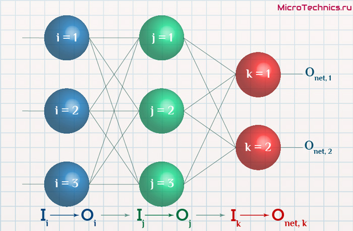
Вернемся к конкретному примеру для явной демонстрации этих принципов:
Итак, имеется нейронная сеть, также имеется набор данных обучающей выборки. Как уже обсудили в начале статьи — обучающая выборка представляет из себя набор образцов (сетов), каждый из которых состоит из значений входных сигналов и соответствующих им «правильных» значений выходных величин.
Процесс обучения нейронной сети для алгоритма обратного распространения ошибки будет таким:
- Прямой проход. Подаем на вход значения I_1, I_2, I_3 из обучающей выборки. В результате работы сети получаем выходные значения O_{net, 1}, O_{net, 2}. Этому целиком и полностью был посвящен предыдущий манускрипт.
- Рассчитываем величины ошибок для всех слоев:
- для выходного: delta_k = (O_{correct, k} — O_{net, k}) cdot f{Large{prime}}(I_k)
- для скрытых: delta_j = (sum_{k}{}{delta_kmedspace w_{jk}}) cdot f{Large{prime}}(I_j)
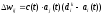
- Далее используем полученные значения для расчета Delta w_{ij} = alpha cdot delta_j cdot O_i + gamma cdot Delta w_{ij}^{t — 1}
- И финишируем, рассчитывая новые значения весов: w_{ij medspace new} = w_{ij} + Delta w_{ij}
- На этом один цикл обучения закончен, данные шаги 1 — 4 повторяются для других образцов из обучающей выборки.
Обратный проход завершен, а вместе с ним и одна итерация процесса обучения нейронной сети по данному методу. Собственно, обучение в целом заключается в многократном повторении этих шагов для разных образцов из обучающей выборки. Логику мы полностью разобрали, при повторном проведении операций она остается в точности такой же.
Таким образом, максимально подробно концентрируясь именно на сути и логике процессов, мы в деталях разобрали метод обратного распространения ошибки. Поэтому переходим к завершающей части статьи, в которой разберем практический пример, произведя полностью все вычисления для конкретных числовых величин. Все в рамках продвигаемой мной концепции, что любая теоретическая информация на порядок лучше может быть осознана при применении ее на практике.
Пример расчетов для метода обратного распространения ошибки.
Возьмем нейронную сеть и зададим начальные значения весов:
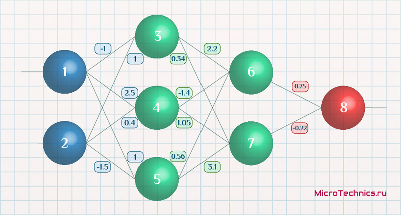
Здесь я задал значения не в соответствии с существующими на сегодняшний день методами, а просто случайным образом для наглядности примера.
В качестве функции активации используем сигмоиду:
f(x) = frac{1}{1 + e^{-x}}
И ее производная:
f{Large{prime}}(x) = f(x)medspace (1medspace-medspace f(x))
Берем один образец из обучающей выборки, пусть будут такие значения:
- Входные: I_1 = 0.6, I_1 = 0.7.
- Выходное: O_{correct} = 0.9.
Скорость обучения alpha пусть будет равна 0.3, момент — gamma = 0.1. Все готово, теперь проведем полный цикл для метода обратного распространения ошибки, то есть прямой проход и обратный.
Прямой проход.
Начинаем с выходных значений нейронов 1 и 2, поскольку они являются входными, то:
O_1 = I_1 = 0.6 \
O_2 = I_2 = 0.7
Значения на входе нейронов 3, 4 и 5:
I_3 = O_1 cdot w_{13} + O_2 cdot w_{23} = 0.6 cdot (-1medspace) + 0.7 cdot 1 = 0.1 \
I_4 = 0.6 cdot 2.5 + 0.7 cdot 0.4 = 1.78 \
I_5 = 0.6 cdot 1 + 0.7 cdot (-1.5medspace) = -0.45
На выходе этих же нейронов первого скрытого слоя:
O_3 = f(I3medspace) = 0.52 \
O_4 = 0.86\
O_5 = 0.39
Продолжаем аналогично для следующего скрытого слоя:
I_6 = O_3 cdot w_{36} + O_4 cdot w_{46} + O_5 cdot w_{56} = 0.52 cdot 2.2 + 0.86 cdot (-1.4medspace) + 0.39 cdot 0.56 = 0.158 \
I_7 = 0.52 cdot 0.34 + 0.86 cdot 1.05 + 0.39 cdot 3.1 = 2.288 \
O_6 = f(I_6) = 0.54 \
O_7 = 0.908
Добрались до выходного нейрона:
I_8 = O_6 cdot w_{68} + O_7 cdot w_{78} = 0.54 cdot 0.75 + 0.908 cdot (-0.22medspace) = 0.205 \
O_8 = O_{net} = f(I_8) = 0.551
Получили значение на выходе сети, кроме того, у нас есть целевое значение O_{correct} = 0.9. То есть все, что необходимо для обратного прохода, имеется.
Обратный проход.
Как мы и обсуждали, первым этапом будет вычисление ошибок всех нейронов, действуем:
delta_8 = (O_{correct} - O_{net}) cdot f{Large{prime}}(I_8) = (O_{correct} - O_{net}) cdot f(I_8) cdot (1-f(I_8)) = (0.9 - 0.551medspace) cdot 0.551 cdot (1-0.551medspace) = 0.0863 \
delta_7 = (sum_{k}{}{delta_kmedspace w_{jk}}) cdot f{Large{prime}}(I_7) = (delta_8 cdot w_{78}) cdot f{Large{prime}}(I_7) = 0.0863 cdot (-0.22medspace) cdot 0.908 cdot (1 - 0.908medspace) = -0.0016 \
delta_6 = 0.086 cdot 0.75 cdot 0.54 cdot (1 - 0.54medspace) = 0.016 \
delta_5 = (sum_{k}{}{delta_kmedspace w_{jk}}) cdot f{Large{prime}}(I_5) = (delta_7 cdot w_{57} + delta_6 cdot w_{56}) cdot f{Large{prime}}(I_7) = (-0.0016 cdot 3.1 + 0.016 cdot 0.56) cdot 0.39 cdot (1 - 0.39medspace) = 0.001 \
delta_4 = (-0.0016 cdot 1.05 + 0.016 cdot (-1.4)) cdot 0.86 cdot (1 - 0.86medspace) = -0.003 \
delta_3 = (-0.0016 cdot 0.34 + 0.016 cdot 2.2) cdot 0.52 cdot (1 - 0.52medspace) = -0.0087
С расчетом ошибок закончили, следующий этап — расчет корректировочных величин для весов всех связей. Для этого мы вывели формулу:
Delta w_{ij} = alpha cdot delta_j cdot O_i + gamma cdot Delta w_{ij}^{t - 1}
Как вы помните, Delta w_{ij}^{t — 1} — это величина поправки для данного веса на предыдущей итерации. Но поскольку у нас это первый проход, то данное значение будет нулевым, соответственно, в данном случае второе слагаемое отпадает. Но забывать о нем нельзя. Продолжаем калькулировать:
Delta w_{78} = alpha cdot delta_8 cdot O_7 = 0.3 cdot 0.0863 cdot 0.908 = 0.0235 \
Delta w_{68} = 0.3 cdot 0.0863 cdot 0.54= 0.014 \
Delta w_{57} = alpha cdot delta_7 cdot O_5 = 0.3 cdot (−0.0016medspace) cdot 0.39= -0.00019 \
Delta w_{47} = 0.3 cdot (−0.0016medspace) cdot 0.86= -0.0004 \
Delta w_{37} = 0.3 cdot (−0.0016medspace) cdot 0.52= -0.00025 \
Delta w_{56} = alpha cdot delta_6 cdot O_5 = 0.3 cdot 0.016 cdot 0.39= 0.0019 \
Delta w_{46} = 0.3 cdot 0.016 cdot 0.86= 0.0041 \
Delta w_{36} = 0.3 cdot 0.016 cdot 0.52= 0.0025 \
Delta w_{25} = alpha cdot delta_5 cdot O_2 = 0.3 cdot 0.001 cdot 0.7= 0.00021 \
Delta w_{15} = 0.3 cdot 0.001 cdot 0.6= 0.00018 \
Delta w_{24} = alpha cdot delta_4 cdot O_2 = 0.3 cdot (-0.003medspace) cdot 0.7= -0.00063 \
Delta w_{14} = 0.3 cdot (-0.003medspace) cdot 0.6= -0.00054 \
Delta w_{23} = alpha cdot delta_3 cdot O_2 = 0.3 cdot (−0.0087medspace) cdot 0.7= -0.00183 \
Delta w_{13} = 0.3 cdot (−0.0087medspace) cdot 0.6= -0.00157
И самый что ни на есть заключительный этап — непосредственно изменение значений весовых коэффициентов:
w_{78 medspace new} = w_{78} + Delta w_{78} = -0.22 + 0.0235 = -0.1965 \
w_{68 medspace new} = 0.75+ 0.014 = 0.764 \
w_{57 medspace new} = 3.1 + (−0.00019medspace) = 3.0998\
w_{47 medspace new} = 1.05 + (−0.0004medspace) = 1.0496\
w_{37 medspace new} = 0.34 + (−0.00025medspace) = 0.3398\
w_{56 medspace new} = 0.56 + 0.0019 = 0.5619 \
w_{46 medspace new} = -1.4 + 0.0041 = -1.3959 \
w_{36 medspace new} = 2.2 + 0.0025 = 2.2025 \
w_{25 medspace new} = -1.5 + 0.00021 = -1.4998 \
w_{15 medspace new} = 1 + 0.00018 = 1.00018 \
w_{24 medspace new} = 0.4 + (−0.00063medspace) = 0.39937 \
w_{14 medspace new} = 2.5 + (−0.00054medspace) = 2.49946 \
w_{23 medspace new} = 1 + (−0.00183medspace) = 0.99817 \
w_{13 medspace new} = -1 + (−0.00157medspace) = -1.00157\
И на этом данную масштабную статью завершаем, конечно же, не завершая на этом деятельность по использованию нейронных сетей. Так что всем спасибо за прочтение, любые вопросы пишите в комментариях и на форуме, ну и обязательно следите за обновлениями и новыми материалами, до встречи!
Нейронные сети обучаются с помощью тех или иных модификаций градиентного спуска, а чтобы применять его, нужно уметь эффективно вычислять градиенты функции потерь по всем обучающим параметрам. Казалось бы, для какого-нибудь запутанного вычислительного графа это может быть очень сложной задачей, но на помощь спешит метод обратного распространения ошибки.
Открытие метода обратного распространения ошибки стало одним из наиболее значимых событий в области искусственного интеллекта. В актуальном виде он был предложен в 1986 году Дэвидом Э. Румельхартом, Джеффри Э. Хинтоном и Рональдом Дж. Вильямсом и независимо и одновременно красноярскими математиками С. И. Барцевым и В. А. Охониным. С тех пор для нахождения градиентов параметров нейронной сети используется метод вычисления производной сложной функции, и оценка градиентов параметров сети стала хоть сложной инженерной задачей, но уже не искусством. Несмотря на простоту используемого математического аппарата, появление этого метода привело к значительному скачку в развитии искусственных нейронных сетей.
Суть метода можно записать одной формулой, тривиально следующей из формулы производной сложной функции: если $f(x) = g_m(g_{m-1}(ldots (g_1(x)) ldots))$, то $frac{partial f}{partial x} = frac{partial g_m}{partial g_{m-1}}frac{partial g_{m-1}}{partial g_{m-2}}ldots frac{partial g_2}{partial g_1}frac{partial g_1}{partial x}$. Уже сейчас мы видим, что градиенты можно вычислять последовательно, в ходе одного обратного прохода, начиная с $frac{partial g_m}{partial g_{m-1}}$ и умножая каждый раз на частные производные предыдущего слоя.
Backpropagation в одномерном случае
В одномерном случае всё выглядит особенно просто. Пусть $w_0$ — переменная, по которой мы хотим продифференцировать, причём сложная функция имеет вид
$$f(w_0) = g_m(g_{m-1}(ldots g_1(w_0)ldots)),$$
где все $g_i$ скалярные. Тогда
$$f'(w_0) = g_m'(g_{m-1}(ldots g_1(w_0)ldots))cdot g’_{m-1}(g_{m-2}(ldots g_1(w_0)ldots))cdotldots cdot g’_1(w_0)$$
Суть этой формулы такова. Если мы уже совершили forward pass, то есть уже знаем
$$g_1(w_0), g_2(g_1(w_0)),ldots,g_{m-1}(ldots g_1(w_0)ldots),$$
то мы действуем следующим образом:
-
берём производную $g_m$ в точке $g_{m-1}(ldots g_1(w_0)ldots)$;
-
умножаем на производную $g_{m-1}$ в точке $g_{m-2}(ldots g_1(w_0)ldots)$;
-
и так далее, пока не дойдём до производной $g_1$ в точке $w_0$.
Проиллюстрируем это на картинке, расписав по шагам дифференцирование по весам $w_i$ функции потерь логистической регрессии на одном объекте (то есть для батча размера 1):
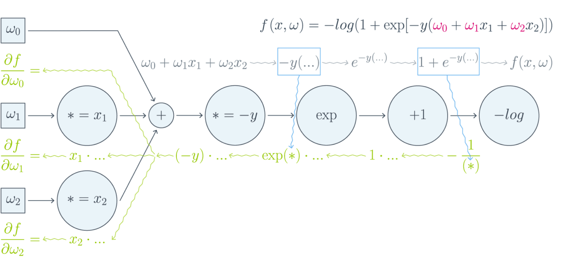
Собирая все множители вместе, получаем:
$$frac{partial f}{partial w_0} = (-y)cdot e^{-y(w_0 + w_1x_1 + w_2x_2)}cdotfrac{-1}{1 + e^{-y(w_0 + w_1x_1 + w_2x_2)}}$$
$$frac{partial f}{partial w_1} = x_1cdot(-y)cdot e^{-y(w_0 + w_1x_1 + w_2x_2)}cdotfrac{-1}{1 + e^{-y(w_0 + w_1x_1 + w_2x_2)}}$$
$$frac{partial f}{partial w_2} = x_2cdot(-y)cdot e^{-y(w_0 + w_1x_1 + w_2x_2)}cdotfrac{-1}{1 + e^{-y(w_0 + w_1x_1 + w_2x_2)}}$$
Таким образом, мы видим, что сперва совершается forward pass для вычисления всех промежуточных значений (и да, все промежуточные представления нужно будет хранить в памяти), а потом запускается backward pass, на котором в один проход вычисляются все градиенты.
Почему же нельзя просто пойти и начать везде вычислять производные?
В главе, посвящённой матричным дифференцированиям, мы поднимаем вопрос о том, что вычислять частные производные по отдельности — это зло, лучше пользоваться матричными вычислениями. Но есть и ещё одна причина: даже и с матричной производной в принципе не всегда хочется иметь дело. Рассмотрим простой пример. Допустим, что $X^r$ и $X^{r+1}$ — два последовательных промежуточных представления $Ntimes M$ и $Ntimes K$, связанных функцией $X^{r+1} = f^{r+1}(X^r)$. Предположим, что мы как-то посчитали производную $frac{partialmathcal{L}}{partial X^{r+1}_{ij}}$ функции потерь $mathcal{L}$, тогда
$$frac{partialmathcal{L}}{partial X^{r}_{st}} = sum_{i,j}frac{partial f^{r+1}_{ij}}{partial X^{r}_{st}}frac{partialmathcal{L}}{partial X^{r+1}_{ij}}$$
И мы видим, что, хотя оба градиента $frac{partialmathcal{L}}{partial X_{ij}^{r+1}}$ и $frac{partialmathcal{L}}{partial X_{st}^{r}}$ являются просто матрицами, в ходе вычислений возникает «четырёхмерный кубик» $frac{partial f_{ij}^{r+1}}{partial X_{st}^{r}}$, даже хранить который весьма болезненно: уж больно много памяти он требует ($N^2MK$ по сравнению с безобидными $NM + NK$, требуемыми для хранения градиентов). Поэтому хочется промежуточные производные $frac{partial f^{r+1}}{partial X^{r}}$ рассматривать не как вычисляемые объекты $frac{partial f_{ij}^{r+1}}{partial X_{st}^{r}}$, а как преобразования, которые превращают $frac{partialmathcal{L}}{partial X_{ij}^{r+1}}$ в $frac{partialmathcal{L}}{partial X_{st}^{r}}$. Целью следующих глав будет именно это: понять, как преобразуется градиент в ходе error backpropagation при переходе через тот или иной слой.
Вы спросите себя: надо ли мне сейчас пойти и прочитать главу учебника про матричное дифференцирование?
Встречный вопрос. Найдите производную функции по вектору $x$:
$$f(x) = x^TAx, Ain Mat_{n}{mathbb{R}}text{ — матрица размера }ntimes n$$
А как всё поменяется, если $A$ тоже зависит от $x$? Чему равен градиент функции, если $A$ является скаляром? Если вы готовы прямо сейчас взять ручку и бумагу и посчитать всё, то вам, вероятно, не надо читать про матричные дифференцирования. Но мы советуем всё-таки заглянуть в эту главу, если обозначения, которые мы будем дальше использовать, покажутся вам непонятными: единой нотации для матричных дифференцирований человечество пока, увы, не изобрело, и переводить с одной на другую не всегда легко.
Мы же сразу перейдём к интересующей нас вещи: к вычислению градиентов сложных функций.
Градиент сложной функции
Напомним, что формула производной сложной функции выглядит следующим образом:
$$left[D_{x_0} (color{#5002A7}{u} circ color{#4CB9C0}{v}) right](h) = color{#5002A7}{left[D_{v(x_0)} u right]} left( color{#4CB9C0}{left[D_{x_0} vright]} (h)right)$$
Теперь разберёмся с градиентами. Пусть $f(x) = g(h(x))$ – скалярная функция. Тогда
$$left[D_{x_0} f right] (x-x_0) = langlenabla_{x_0} f, x-x_0rangle.$$
С другой стороны,
$$left[D_{h(x_0)} g right] left(left[D_{x_0}h right] (x-x_0)right) = langlenabla_{h_{x_0}} g, left[D_{x_0} hright] (x-x_0)rangle = langleleft[D_{x_0} hright]^* nabla_{h(x_0)} g, x-x_0rangle.$$
То есть $color{#FFC100}{nabla_{x_0} f} = color{#348FEA}{left[D_{x_0} h right]}^* color{#FFC100}{nabla_{h(x_0)}}g$ — применение сопряжённого к $D_{x_0} h$ линейного отображения к вектору $nabla_{h(x_0)} g$.
Эта формула — сердце механизма обратного распространения ошибки. Она говорит следующее: если мы каким-то образом получили градиент функции потерь по переменным из некоторого промежуточного представления $X^k$ нейронной сети и при этом знаем, как преобразуется градиент при проходе через слой $f^k$ между $X^{k-1}$ и $X^k$ (то есть как выглядит сопряжённое к дифференциалу слоя между ними отображение), то мы сразу же находим градиент и по переменным из $X^{k-1}$:
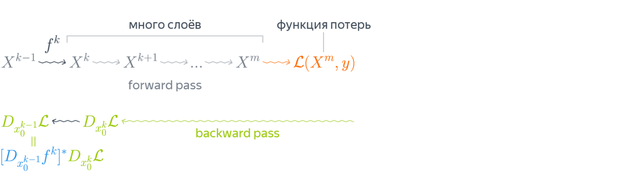
Таким образом слой за слоем мы посчитаем градиенты по всем $X^i$ вплоть до самых первых слоёв.
Далее мы разберёмся, как именно преобразуются градиенты при переходе через некоторые распространённые слои.
Градиенты для типичных слоёв
Рассмотрим несколько важных примеров.
Примеры
-
$f(x) = u(v(x))$, где $x$ — вектор, а $v(x)$ – поэлементное применение $v$:
$$vbegin{pmatrix}
x_1
vdots
x_N
end{pmatrix}
= begin{pmatrix}
v(x_1)
vdots
v(x_N)
end{pmatrix}$$Тогда, как мы знаем,
$$left[D_{x_0} fright] (h) = langlenabla_{x_0} f, hrangle = left[nabla_{x_0} fright]^T h.$$
Следовательно,
$$begin{multline*}
left[D_{v(x_0)} uright] left( left[ D_{x_0} vright] (h)right) = left[nabla_{v(x_0)} uright]^T left(v'(x_0) odot hright) =\[0.1cm]
= sumlimits_i left[nabla_{v(x_0)} uright]_i v'(x_{0i})h_i
= langleleft[nabla_{v(x_0)} uright] odot v'(x_0), hrangle.
end{multline*},$$где $odot$ означает поэлементное перемножение. Окончательно получаем
$$color{#348FEA}{nabla_{x_0} f = left[nabla_{v(x_0)}uright] odot v'(x_0) = v'(x_0) odot left[nabla_{v(x_0)} uright]}$$
Отметим, что если $x$ и $h(x)$ — это просто векторы, то мы могли бы вычислять всё и по формуле $frac{partial f}{partial x_i} = sum_jbig(frac{partial z_j}{partial x_i}big)cdotbig(frac{partial h}{partial z_j}big)$. В этом случае матрица $big(frac{partial z_j}{partial x_i}big)$ была бы диагональной (так как $z_j$ зависит только от $x_j$: ведь $h$ берётся поэлементно), и матричное умножение приводило бы к тому же результату. Однако если $x$ и $h(x)$ — матрицы, то $big(frac{partial z_j}{partial x_i}big)$ представлялась бы уже «четырёхмерным кубиком», и работать с ним было бы ужасно неудобно.
-
$f(X) = g(XW)$, где $X$ и $W$ — матрицы. Как мы знаем,
$$left[D_{X_0} f right] (X-X_0) = text{tr}, left(left[nabla_{X_0} fright]^T (X-X_0)right).$$
Тогда
$$begin{multline*}
left[ D_{X_0W} g right] left(left[D_{X_0} left( ast Wright)right] (H)right) =
left[ D_{X_0W} g right] left(HWright)=\
= text{tr}, left( left[nabla_{X_0W} g right]^T cdot (H) W right) =\
=
text{tr} , left(W left[nabla_{X_0W} (g) right]^T cdot (H)right) = text{tr} , left( left[left[nabla_{X_0W} gright] W^Tright]^T (H)right)
end{multline*}$$Здесь через $ast W$ мы обозначили отображение $Y hookrightarrow YW$, а в предпоследнем переходе использовалось следующее свойство следа:
$$
text{tr} , (A B C) = text{tr} , (C A B),
$$где $A, B, C$ — произвольные матрицы подходящих размеров (то есть допускающие перемножение в обоих приведённых порядках). Следовательно, получаем
$$color{#348FEA}{nabla_{X_0} f = left[nabla_{X_0W} (g) right] cdot W^T}$$
-
$f(W) = g(XW)$, где $W$ и $X$ — матрицы. Для приращения $H = W — W_0$ имеем
$$
left[D_{W_0} f right] (H) = text{tr} , left( left[nabla_{W_0} f right]^T (H)right)
$$Тогда
$$ begin{multline*}
left[D_{XW_0} g right] left( left[D_{W_0} left(X astright) right] (H)right) = left[D_{XW_0} g right] left( XH right) =
= text{tr} , left( left[nabla_{XW_0} g right]^T cdot X (H)right) =
text{tr}, left(left[X^T left[nabla_{XW_0} g right] right]^T (H)right)
end{multline*} $$Здесь через $X ast$ обозначено отображение $Y hookrightarrow XY$. Значит,
$$color{#348FEA}{nabla_{X_0} f = X^T cdot left[nabla_{XW_0} (g)right]}$$
-
$f(X) = g(softmax(X))$, где $X$ — матрица $Ntimes K$, а $softmax$ — функция, которая вычисляется построчно, причём для каждой строки $x$
$$softmax(x) = left(frac{e^{x_1}}{sum_te^{x_t}},ldots,frac{e^{x_K}}{sum_te^{x_t}}right)$$
В этом примере нам будет удобно воспользоваться формализмом с частными производными. Сначала вычислим $frac{partial s_l}{partial x_j}$ для одной строки $x$, где через $s_l$ мы для краткости обозначим $softmax(x)_l = frac{e^{x_l}} {sum_te^{x_t}}$. Нетрудно проверить, что
$$frac{partial s_l}{partial x_j} = begin{cases}
s_j(1 — s_j), & j = l,
-s_ls_j, & jne l
end{cases}$$Так как softmax вычисляется независимо от каждой строчки, то
$$frac{partial s_{rl}}{partial x_{ij}} = begin{cases}
s_{ij}(1 — s_{ij}), & r=i, j = l,
-s_{il}s_{ij}, & r = i, jne l,
0, & rne i
end{cases},$$где через $s_{rl}$ мы обозначили для краткости $softmax(X)_{rl}$.
Теперь пусть $nabla_{rl} = nabla g = frac{partialmathcal{L}}{partial s_{rl}}$ (пришедший со следующего слоя, уже известный градиент). Тогда
$$frac{partialmathcal{L}}{partial x_{ij}} = sum_{r,l}frac{partial s_{rl}}{partial x_{ij}} nabla_{rl}$$
Так как $frac{partial s_{rl}}{partial x_{ij}} = 0$ при $rne i$, мы можем убрать суммирование по $r$:
$$ldots = sum_{l}frac{partial s_{il}}{partial x_{ij}} nabla_{il} = -s_{i1}s_{ij}nabla_{i1} — ldots + s_{ij}(1 — s_{ij})nabla_{ij}-ldots — s_{iK}s_{ij}nabla_{iK} =$$
$$= -s_{ij}sum_t s_{it}nabla_{it} + s_{ij}nabla_{ij}$$
Таким образом, если мы хотим продифференцировать $f$ в какой-то конкретной точке $X_0$, то, смешивая математические обозначения с нотацией Python, мы можем записать:
$$begin{multline*}
color{#348FEA}{nabla_{X_0}f =}\
color{#348FEA}{= -softmax(X_0) odot text{sum}left(
softmax(X_0)odotnabla_{softmax(X_0)}g, text{ axis = 1}
right) +}\
color{#348FEA}{softmax(X_0)odot nabla_{softmax(X_0)}g}
end{multline*}
$$
Backpropagation в общем виде
Подытожим предыдущее обсуждение, описав алгоритм error backpropagation (алгоритм обратного распространения ошибки). Допустим, у нас есть текущие значения весов $W^i_0$ и мы хотим совершить шаг SGD по мини-батчу $X$. Мы должны сделать следующее:
- Совершить forward pass, вычислив и запомнив все промежуточные представления $X = X^0, X^1, ldots, X^m = widehat{y}$.
- Вычислить все градиенты с помощью backward pass.
- С помощью полученных градиентов совершить шаг SGD.
Проиллюстрируем алгоритм на примере двуслойной нейронной сети со скалярным output’ом. Для простоты опустим свободные члены в линейных слоях.
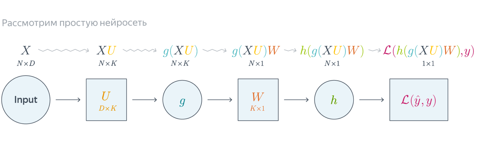 Обучаемые параметры – матрицы $U$ и $W$. Как найти градиенты по ним в точке $U_0, W_0$?
$$nabla_{W_0}mathcal{L} = nabla_{W_0}{left({vphantom{frac12}mathcal{L}circ hcircleft[Wmapsto g(XU_0)Wright]}right)}=$$
$$=g(XU_0)^Tnabla_{g(XU_0)W_0}(mathcal{L}circ h) = underbrace{g(XU_0)^T}_{ktimes N}cdot
left[vphantom{frac12}underbrace{h’left(vphantom{int_0^1}g(XU_0)W_0right)}_{Ntimes 1}odot
underbrace{nabla_{hleft(vphantom{int_0^1}g(XU_0)W_0right)}mathcal{L}}_{Ntimes 1}right]$$
Итого матрица $ktimes 1$, как и $W_0$
$$nabla_{U_0}mathcal{L} = nabla_{U_0}left(vphantom{frac12}
mathcal{L}circ hcircleft[Ymapsto YW_0right]circ gcircleft[ Umapsto XUright]
right)=$$
$$=X^Tcdotnabla_{XU^0}left(vphantom{frac12}mathcal{L}circ hcirc [Ymapsto YW_0]circ gright) =$$
$$=X^Tcdotleft(vphantom{frac12}g'(XU_0)odot
nabla_{g(XU_0)}left[vphantom{in_0^1}mathcal{L}circ hcirc[Ymapsto YW_0right]
right)$$
$$=ldots = underset{Dtimes N}{X^T}cdotleft(vphantom{frac12}
underbrace{g'(XU_0)}_{Ntimes K}odot
underbrace{left[vphantom{int_0^1}left(
underbrace{h’left(vphantom{int_0^1}g(XU_0)W_0right)}_{Ntimes1}odotunderbrace{nabla_{h(vphantom{int_0^1}gleft(XU_0right)W_0)}mathcal{L}}_{Ntimes 1}
right)cdot underbrace{W^T}_{1times K}right]}_{Ntimes K}
right)$$
Итого $Dtimes K$, как и $U_0$
Схематически это можно представить следующим образом:
Backpropagation для двуслойной нейронной сети
Если вы не уследили за вычислениями в предыдущем примере, давайте более подробно разберём его чуть более конкретную версию (для $g = h = sigma$)Рассмотрим двуслойную нейронную сеть для классификации. Мы уже встречали ее ранее при рассмотрении линейно неразделимой выборки. Предсказания получаются следующим образом:
$$
widehat{y} = sigma(X^1 W^2) = sigmaBig(big(sigma(X^0 W^1 )big) W^2 Big).
$$
Пусть $W^1_0$ и $W^2_0$ — текущее приближение матриц весов. Мы хотим совершить шаг по градиенту функции потерь, и для этого мы должны вычислить её градиенты по $W^1$ и $W^2$ в точке $(W^1_0, W^2_0)$.
Прежде всего мы совершаем forward pass, в ходе которого мы должны запомнить все промежуточные представления: $X^1 = X^0 W^1_0$, $X^2 = sigma(X^0 W^1_0)$, $X^3 = sigma(X^0 W^1_0) W^2_0$, $X^4 = sigma(sigma(X^0 W^1_0) W^2_0) = widehat{y}$. Они понадобятся нам дальше.
Для полученных предсказаний вычисляется значение функции потерь:
$$
l = mathcal{L}(y, widehat{y}) = y log(widehat{y}) + (1-y) log(1-widehat{y}).
$$
Дальше мы шаг за шагом будем находить производные по переменным из всё более глубоких слоёв.
-
Градиент $mathcal{L}$ по предсказаниям имеет вид
$$
nabla_{widehat{y}}l = frac{y}{widehat{y}} — frac{1 — y}{1 — widehat{y}} = frac{y — widehat{y}}{widehat{y} (1 — widehat{y})},
$$где, напомним, $ widehat{y} = sigma(X^3) = sigmaBig(big(sigma(X^0 W^1_0 )big) W^2_0 Big)$ (обратите внимание на то, что $W^1_0$ и $W^2_0$ тут именно те, из которых мы делаем градиентный шаг).
-
Следующий слой — поэлементное взятие $sigma$. Как мы помним, при переходе через него градиент поэлементно умножается на производную $sigma$, в которую подставлено предыдущее промежуточное представление:
$$
nabla_{X^3}l = sigma'(X^3)odotnabla_{widehat{y}}l = sigma(X^3)left( 1 — sigma(X^3) right) odot frac{y — widehat{y}}{widehat{y} (1 — widehat{y})} =
$$$$
= sigma(X^3)left( 1 — sigma(X^3) right) odot frac{y — sigma(X^3)}{sigma(X^3) (1 — sigma(X^3))} =
y — sigma(X^3)
$$ -
Следующий слой — умножение на $W^2_0$. В этот момент мы найдём градиент как по $W^2$, так и по $X^2$. При переходе через умножение на матрицу градиент, как мы помним, умножается с той же стороны на транспонированную матрицу, а значит:
$$
color{blue}{nabla_{W^2_0}l} = (X^2)^Tcdot nabla_{X^3}l = (X^2)^Tcdot(y — sigma(X^3)) =
$$$$
= color{blue}{left( sigma(X^0W^1_0) right)^T cdot (y — sigma(sigma(X^0W^1_0)W^2_0))}
$$Аналогичным образом
$$
nabla_{X^2}l = nabla_{X^3}lcdot (W^2_0)^T = (y — sigma(X^3))cdot (W^2_0)^T =
$$$$
= (y — sigma(X^2W_0^2))cdot (W^2_0)^T
$$ -
Следующий слой — снова взятие $sigma$.
$$
nabla_{X^1}l = sigma'(X^1)odotnabla_{X^2}l = sigma(X^1)left( 1 — sigma(X^1) right) odot left( (y — sigma(X^2W_0^2))cdot (W^2_0)^T right) =
$$$$
= sigma(X^1)left( 1 — sigma(X^1) right) odotleft( (y — sigma(sigma(X^1)W_0^2))cdot (W^2_0)^T right)
$$ -
Наконец, последний слой — это умножение $X^0$ на $W^1_0$. Тут мы дифференцируем только по $W^1$:
$$
color{blue}{nabla_{W^1_0}l} = (X^0)^Tcdot nabla_{X^1}l = (X^0)^Tcdot big( sigma(X^1) left( 1 — sigma(X^1) right) odot (y — sigma(sigma(X^1)W_0^2))cdot (W^2_0)^Tbig) =
$$$$
= color{blue}{(X^0)^Tcdotbig(sigma(X^0W^1_0)left( 1 — sigma(X^0W^1_0) right) odot (y — sigma(sigma(X^0W^1_0)W_0^2))cdot (W^2_0)^Tbig) }
$$
Итоговые формулы для градиентов получились страшноватыми, но они были получены друг из друга итеративно с помощью очень простых операций: матричного и поэлементного умножения, в которые порой подставлялись значения заранее вычисленных промежуточных представлений.
Автоматизация и autograd
Итак, чтобы нейросеть обучалась, достаточно для любого слоя $f^k: X^{k-1}mapsto X^k$ с параметрами $W^k$ уметь:
- превращать $nabla_{X^k_0}mathcal{L}$ в $nabla_{X^{k-1}_0}mathcal{L}$ (градиент по выходу в градиент по входу);
- считать градиент по его параметрам $nabla_{W^k_0}mathcal{L}$.
При этом слою совершенно не надо знать, что происходит вокруг. То есть слой действительно может быть запрограммирован как отдельная сущность, умеющая внутри себя делать forward pass и backward pass, после чего слои механически, как кубики в конструкторе, собираются в большую сеть, которая сможет работать как одно целое.
Более того, во многих случаях авторы библиотек для глубинного обучения уже о вас позаботились и создали средства для автоматического дифференцирования выражений (autograd). Поэтому, программируя нейросеть, вы почти всегда можете думать только о forward-проходе, прямом преобразовании данных, предоставив библиотеке дифференцировать всё самостоятельно. Это делает код нейросетей весьма понятным и выразительным (да, в реальности он тоже бывает большим и страшным, но сравните на досуге код какой-нибудь разухабистой нейросети и код градиентного бустинга на решающих деревьях и почувствуйте разницу).
Но это лишь начало
Метод обратного распространения ошибки позволяет удобно посчитать градиенты, но дальше с ними что-то надо делать, и старый добрый SGD едва ли справится с обучением современной сетки. Так что же делать? О некоторых приёмах мы расскажем в следующей главе.
4.2.1. Дельта-правило
Дельта-правило. Стимулом для обучения
является рассогласование
 между некоторым заданным обучающим
сигналом и текущей активностью постсинаптического
нейрона ai
 .
.
(4.15)
Дельта-правило в виде конечно-разностного
уравнения записывается следующим
образом
 ,
,
(4.16)
где i(t)
— ошибка выхода i-го нейрона
(постсинаптического), равная разности
между i-ой компонентой k-го целевого
вектора из множества D и активностью
i-го нейрона.
Очевидно, что если
 >ai(t),
весовые коэффициенты будут увеличены
и тем самым уменьшат ошибку. В противном
случае они уменьшаться и активность
нейрона тоже уменьшиться, приближаясь
к компоненте целевого вектора.
4.2.2. Правило обратного распространения ошибки
Если сеть является многослойной, то
ошибку для скрытых слоев невозможно
задать в явном виде. В этом случае для
расчета величины рассогласования
используется обобщение Дельта-правила
– правило обратного распространения
ошибки (Вр-алгоритм). На авторство этого
алгоритма претендуют трое ученых:
Румелхарт (1986), Паркер (1982), Вербос (1974).
В Вр-алгоритме используются два уравнения
для вычисления величины коррекции
весов.
Если i-ый нейрон (постсинаптический)
является выходным, то используется
измененное Дельта-правило с иным методом
вычисления ошибки
 .
.
(4.21)
Если нейрон является скрытым Дельта-правило
преобразуется к следующему виду
 ,
,
(4.22)
где p(t) –
ошибка для p-го нейрона следующего слоя;
wpi– вес синаптической связи от
i-го нейрона к p-му нейрону следующего
слоя (рис. 4.13).
Корректировка пороговых величин нейронов
выполняется также в обратном направлении
 .
.
(4.23)
Здесь также величина ошибки вычисляется
исходя из того, в каком слое находится
нейрон.
Конечно-разностное уравнение Вр-алгоритма
совпадает с соответствующим уравнением
Дельта-правила (4.16) за исключением метода
расчета ошибки.
Недостатки Вр-алгоритма
1. Паралич сети (блокировка обучения).
2. Попадание сети в локальные минимумы.
3. Переобучение.
4. Медленная сходимость процесса обучения.
Модификации Вр-алгоритма
1. Импульсный метод экспоненциального
сглаживания.
Для придания процессу коррекции весов
некоторой инерционности Вр-алгоритм
дополняется значением изменения веса
на предыдущей итерации
 ,
,
(4.24)
где – коэффициент
инерционности (сглаживания), устанавливается
от 0 до 1 (обычно около 0,9). Еслиравен 1, то новая коррекция игнорируется
и повторяется предыдущая.
2. Квадратичный метод (квазиньютоновский
метод и метод сопряженных градиентов).
Разработан метод ускорения обучения,
основанный на вычислении вторых
производных для более точной оценки
требуемой коррекции весов (Паркер,
1987г.).
3.Использование симметричного диапазона
изменения весов.
Симметричный диапазон изменения весов
и сигналов в сети (например, от -1 до 1)
дает прирост скорости обучения на 30-50%
(Сторнетта, Хьюберман, 1987г.). Функция
активации при этом должна быть симметричной
(например, гиперболический тангенс).
Когда выходное значение aj(n-1)стремится к нулю, эффективность обучения
заметно снижается. При двоичных входных
векторах половина входов в среднем
будет равна нулю, и веса, с которыми они
связаны, не будут обучаться, поэтому
область возможных значений выходов
нейронов [0,1] желательно сдвинуть в
пределы [-0.5,+0.5], что достигается простыми
модификациями логистических функций.
Например, сигмоидальная функция
преобразуется к виду
 .
.
(4.25)
4. Использование различных функций
вычисления ошибок (для ускорения процесса
обучения):
интегральные функции ошибки по
всей совокупности обучающих примеров;
функции ошибки целых и дробных
степеней.
5. Использование различных процедур
определения величины шага (скорости
обучения) на каждой итерации:
расписание обучения (с=с(t));
скорость обучения выбирают различной
для каждого слоя;
дихотомия;
инерционные соотношения для
предотвращения блокировки сети, например,
 ,
,
(4.26)
где <1 — некоторое
положительное число, меньше единицы;
отжиг.
6. Использование различных
процедур определения направления шага:
с использованием матрицы производных
второго порядка (метод Ньютона и др.);
с использованием направлений на
нескольких шагах.
Алгоритм обучения НС с помощью процедуры
обратного распространения следующий
(при условии, что ошибка вычисляется по
единичным примерам).
1. На стации инициализации всем весовым
коэффициентам и пороговым значениям
присваиваются небольшие случайные
значения.
2. На входы сети подается очередной
входной образ из ОВ.
3. Сигналы возбуждения распространяются
по всем слоям сети в прямом направлении.
В процессе прохождения сигнала вычисляются
значения активностей постсинаптических
нейронов.
4. Вычисляется ошибка сети и значения
приращения весовых коэффициентов для
всех синаптических связей выходного
слоя сети.
5. Корректируются весовые коэффициенты
нейронов выходного слоя сети.
6. Выполняется переход к предыдущему
слою. Вычисляются значения приращения
весов для всех синаптических связей
текущего слоя сети (обратное распространение
ошибки).
7. Корректируются весовые коэффициенты
нейронов текущего скрытого слоя сети.
8. Шаги 6-7 повторяются, пока не будут
пройдены все слои НС. Аналогичные
вычисления выполняются и для пороговых
значений.
9. Шаги 2-9 повторяются для всех примеров
ОВ.
10. Рассчитывается суммарная ошибка
сети.
11. Если вычисленная ошибка существенна,
перейти на шаг 2. В противном случае –
конец.
Соседние файлы в папке конспекты лекций
- #
- #
- #
- #
- #
- #
This article is about the computer algorithm. For the biological process, see neural backpropagation.
Backpropagation can also refer to the way the result of a playout is propagated up the search tree in Monte Carlo tree search.
In machine learning, backpropagation (backprop,[1] BP) is a widely used algorithm for training feedforward artificial neural networks. Generalizations of backpropagation exist for other artificial neural networks (ANNs), and for functions generally. These classes of algorithms are all referred to generically as «backpropagation».[2] In fitting a neural network, backpropagation computes the gradient of the loss function with respect to the weights of the network for a single input–output example, and does so efficiently, unlike a naive direct computation of the gradient with respect to each weight individually. This efficiency makes it feasible to use gradient methods for training multilayer networks, updating weights to minimize loss; gradient descent, or variants such as stochastic gradient descent, are commonly used. The backpropagation algorithm works by computing the gradient of the loss function with respect to each weight by the chain rule, computing the gradient one layer at a time, iterating backward from the last layer to avoid redundant calculations of intermediate terms in the chain rule; this is an example of dynamic programming.[3]
The term backpropagation strictly refers only to the algorithm for computing the gradient, not how the gradient is used; however, the term is often used loosely to refer to the entire learning algorithm, including how the gradient is used, such as by stochastic gradient descent.[4] Backpropagation generalizes the gradient computation in the delta rule, which is the single-layer version of backpropagation, and is in turn generalized by automatic differentiation, where backpropagation is a special case of reverse accumulation (or «reverse mode»).[5] The term backpropagation and its general use in neural networks was announced in Rumelhart, Hinton & Williams (1986a), then elaborated and popularized in Rumelhart, Hinton & Williams (1986b), but the technique was independently rediscovered many times, and had many predecessors dating to the 1960s; see § History.[6] A modern overview is given in the deep learning textbook by Goodfellow, Bengio & Courville (2016).[7]
Overview[edit]
Backpropagation computes the gradient in weight space of a feedforward neural network, with respect to a loss function. Denote:
 : input (vector of features)
- : target output
- For classification, output will be a vector of class probabilities (e.g., , and target output is a specific class, encoded by the one-hot/dummy variable (e.g., ).
- For classification, output will be a vector of class probabilities (e.g.,
- : loss function or «cost function»[a]
- For classification, this is usually cross entropy (XC, log loss), while for regression it is usually squared error loss (SEL).
- : the number of layers
- : the weights between layer and , where is the weight between the -th node in layer and the -th node in layer [b]
- : activation functions at layer
- For classification the last layer is usually the logistic function for binary classification, and softmax (softargmax) for multi-class classification, while for the hidden layers this was traditionally a sigmoid function (logistic function or others) on each node (coordinate), but today is more varied, with rectifier (ramp, ReLU) being common.


In the derivation of backpropagation, other intermediate quantities are used; they are introduced as needed below. Bias terms are not treated specially, as they correspond to a weight with a fixed input of 1. For the purpose of backpropagation, the specific loss function and activation functions do not matter, as long as they and their derivatives can be evaluated efficiently. Traditional activation functions include but are not limited to sigmoid, tanh, and ReLU. Since, swish,[8] mish,[9] and other activation functions were proposed as well.
The overall network is a combination of function composition and matrix multiplication:

For a training set there will be a set of input–output pairs,  . For each input–output pair
  in the training set, the loss of the model on that pair is the cost of the difference between the predicted output
  and the target output
  :
:

Note the distinction: during model evaluation, the weights are fixed, while the inputs vary (and the target output may be unknown), and the network ends with the output layer (it does not include the loss function). During model training, the input–output pair is fixed, while the weights vary, and the network ends with the loss function.
Backpropagation computes the gradient for a fixed input–output pair , where the weights  can vary. Each individual component of the gradient,
  can be computed by the chain rule; however, doing this separately for each weight is inefficient. Backpropagation efficiently computes the gradient by avoiding duplicate calculations and not computing unnecessary intermediate values, by computing the gradient of each layer – specifically, the gradient of the weighted input of each layer, denoted by
  – from back to front.
Informally, the key point is that since the only way a weight in  affects the loss is through its effect on the next layer, and it does so linearly, are the only data you need to compute the gradients of the weights at layer
  , and then you can compute the previous layer
  and repeat recursively. This avoids inefficiency in two ways. Firstly, it avoids duplication because when computing the gradient at layer , you do not need to recompute all the derivatives on later layers
  each time. Secondly, it avoids unnecessary intermediate calculations because at each stage it directly computes the gradient of the weights with respect to the ultimate output (the loss), rather than unnecessarily computing the derivatives of the values of hidden layers with respect to changes in weights
  .
.
Backpropagation can be expressed for simple feedforward networks in terms of matrix multiplication, or more generally in terms of the adjoint graph.
Matrix multiplication[edit]
For the basic case of a feedforward network, where nodes in each layer are connected only to nodes in the immediate next layer (without skipping any layers), and there is a loss function that computes a scalar loss for the final output, backpropagation can be understood simply by matrix multiplication.[c] Essentially, backpropagation evaluates the expression for the derivative of the cost function as a product of derivatives between each layer from right to left – «backwards» – with the gradient of the weights between each layer being a simple modification of the partial products (the «backwards propagated error»).
Given an input–output pair  , the loss is:

To compute this, one starts with the input  and works forward; denote the weighted input of each hidden layer as
  and the output of hidden layer as the activation
  . For backpropagation, the activation as well as the derivatives
  (evaluated at ) must be cached for use during the backwards pass.
The derivative of the loss in terms of the inputs is given by the chain rule; note that each term is a total derivative, evaluated at the value of the network (at each node) on the input :

where  is a Hadamard product, that is an element-wise product.
These terms are: the derivative of the loss function;[d] the derivatives of the activation functions;[e] and the matrices of weights:[f]

The gradient  is the transpose of the derivative of the output in terms of the input, so the matrices are transposed and the order of multiplication is reversed, but the entries are the same:

Backpropagation then consists essentially of evaluating this expression from right to left (equivalently, multiplying the previous expression for the derivative from left to right), computing the gradient at each layer on the way; there is an added step, because the gradient of the weights isn’t just a subexpression: there’s an extra multiplication.
Introducing the auxiliary quantity for the partial products (multiplying from right to left), interpreted as the «error at level » and defined as the gradient of the input values at level :

Note that is a vector, of length equal to the number of nodes in level ; each component is interpreted as the «cost attributable to (the value of) that node».
The gradient of the weights in layer is then:

The factor of  is because the weights between level
  and affect level proportionally to the inputs (activations): the inputs are fixed, the weights vary.
The can easily be computed recursively, going from right to left, as:

The gradients of the weights can thus be computed using a few matrix multiplications for each level; this is backpropagation.
Compared with naively computing forwards (using the for illustration):

there are two key differences with backpropagation:
- Computing in terms of avoids the obvious duplicate multiplication of layers and beyond.
- Multiplying starting from – propagating the error backwards – means that each step simply multiplies a vector () by the matrices of weights and derivatives of activations . By contrast, multiplying forwards, starting from the changes at an earlier layer, means that each multiplication multiplies a matrix by a matrix. This is much more expensive, and corresponds to tracking every possible path of a change in one layer forward to changes in the layer (for multiplying by , with additional multiplications for the derivatives of the activations), which unnecessarily computes the intermediate quantities of how weight changes affect the values of hidden nodes.


Adjoint graph[edit]
|
This section needs expansion. You can help by adding to it. (November 2019) |
For more general graphs, and other advanced variations, backpropagation can be understood in terms of automatic differentiation, where backpropagation is a special case of reverse accumulation (or «reverse mode»).[5]
Intuition[edit]
Motivation[edit]
The goal of any supervised learning algorithm is to find a function that best maps a set of inputs to their correct output. The motivation for backpropagation is to train a multi-layered neural network such that it can learn the appropriate internal representations to allow it to learn any arbitrary mapping of input to output.[10]
Learning as an optimization problem[edit]
To understand the mathematical derivation of the backpropagation algorithm, it helps to first develop some intuition about the relationship between the actual output of a neuron and the correct output for a particular training example. Consider a simple neural network with two input units, one output unit and no hidden units, and in which each neuron uses a linear output (unlike most work on neural networks, in which mapping from inputs to outputs is non-linear)[g] that is the weighted sum of its input.

A simple neural network with two input units (each with a single input) and one output unit (with two inputs)
Initially, before training, the weights will be set randomly. Then the neuron learns from training examples, which in this case consist of a set of tuples  where
where  and
and  are the inputs to the network and t is the correct output (the output the network should produce given those inputs, when it has been trained). The initial network, given and , will compute an output y that likely differs from t (given random weights). A loss function
  is used for measuring the discrepancy between the target output t and the computed output y. For regression analysis problems the squared error can be used as a loss function, for classification the categorical crossentropy can be used.
As an example consider a regression problem using the square error as a loss:

where E is the discrepancy or error.
Consider the network on a single training case:  . Thus, the input and are 1 and 1 respectively and the correct output, t is 0. Now if the relation is plotted between the network’s output y on the horizontal axis and the error E on the vertical axis, the result is a parabola. The minimum of the parabola corresponds to the output y which minimizes the error E. For a single training case, the minimum also touches the horizontal axis, which means the error will be zero and the network can produce an output y that exactly matches the target output t. Therefore, the problem of mapping inputs to outputs can be reduced to an optimization problem of finding a function that will produce the minimal error.

Error surface of a linear neuron for a single training case
However, the output of a neuron depends on the weighted sum of all its inputs:

where  and
and  are the weights on the connection from the input units to the output unit. Therefore, the error also depends on the incoming weights to the neuron, which is ultimately what needs to be changed in the network to enable learning.
In this example, upon injecting the training data , the loss function becomes

Then, the loss function  takes the form of a parabolic cylinder with its base directed along
  . Since all sets of weights that satisfy minimize the loss function, in this case additional constraints are required to converge to a unique solution. Additional constraints could either be generated by setting specific conditions to the weights, or by injecting additional training data.
One commonly used algorithm to find the set of weights that minimizes the error is gradient descent. By backpropagation, the steepest descent direction is calculated of the loss function versus the present synaptic weights. Then, the weights can be modified along the steepest descent direction, and the error is minimized in an efficient way.
Derivation[edit]
The gradient descent method involves calculating the derivative of the loss function with respect to the weights of the network. This is normally done using backpropagation. Assuming one output neuron,[h] the squared error function is

where
- is the loss for the output and target value ,
- is the target output for a training sample, and
- is the actual output of the output neuron.

For each neuron  , its output
  is defined as

where the activation function  is non-linear and differentiable over the activation region (the ReLU is not differentiable at one point). A historically used activation function is the logistic function:

which has a convenient derivative of:

The input  to a neuron is the weighted sum of outputs
  of previous neurons. If the neuron is in the first layer after the input layer, the of the input layer are simply the inputs
  to the network. The number of input units to the neuron is
  . The variable
  denotes the weight between neuron
  of the previous layer and neuron of the current layer.
Finding the derivative of the error[edit]

Diagram of an artificial neural network to illustrate the notation used here
Calculating the partial derivative of the error with respect to a weight  is done using the chain rule twice:
-
(Eq. 1)

In the last factor of the right-hand side of the above, only one term in the sum depends on , so that
-
(Eq. 2)

If the neuron is in the first layer after the input layer,  is just
  .
.
The derivative of the output of neuron with respect to its input is simply the partial derivative of the activation function:
-
(Eq. 3)

which for the logistic activation function

This is the reason why backpropagation requires the activation function to be differentiable. (Nevertheless, the ReLU activation function, which is non-differentiable at 0, has become quite popular, e.g. in AlexNet)
The first factor is straightforward to evaluate if the neuron is in the output layer, because then  and
and
-
(Eq. 4)

If half of the square error is used as loss function we can rewrite it as

However, if is in an arbitrary inner layer of the network, finding the derivative with respect to is less obvious.
Considering as a function with the inputs being all neurons  receiving input from neuron ,

and taking the total derivative with respect to , a recursive expression for the derivative is obtained:
-
(Eq. 5)

Therefore, the derivative with respect to can be calculated if all the derivatives with respect to the outputs  of the next layer – the ones closer to the output neuron – are known. [Note, if any of the neurons in set
  were not connected to neuron , they would be independent of and the corresponding partial derivative under the summation would vanish to 0.]
Substituting Eq. 2, Eq. 3 Eq.4 and Eq. 5 in Eq. 1 we obtain:


with

if is the logistic function, and the error is the square error:

To update the weight using gradient descent, one must choose a learning rate,  . The change in weight needs to reflect the impact on of an increase or decrease in . If
  , an increase in increases ; conversely, if
  , an increase in decreases . The new
  is added to the old weight, and the product of the learning rate and the gradient, multiplied by
  guarantees that changes in a way that always decreases . In other words, in the equation immediately below,
  always changes in such a way that is decreased:

Second-order gradient descent[edit]
Using a Hessian matrix of second-order derivatives of the error function, the Levenberg-Marquardt algorithm often converges faster than first-order gradient descent, especially when the topology of the error function is complicated.[11][12] It may also find solutions in smaller node counts for which other methods might not converge.[12] The Hessian can be approximated by the Fisher information matrix.[13]
Loss function[edit]
The loss function is a function that maps values of one or more variables onto a real number intuitively representing some «cost» associated with those values. For backpropagation, the loss function calculates the difference between the network output and its expected output, after a training example has propagated through the network.
Assumptions[edit]
The mathematical expression of the loss function must fulfill two conditions in order for it to be possibly used in backpropagation.[14] The first is that it can be written as an average  over error functions
  , for
, for  individual training examples,
  . The reason for this assumption is that the backpropagation algorithm calculates the gradient of the error function for a single training example, which needs to be generalized to the overall error function. The second assumption is that it can be written as a function of the outputs from the neural network.
Example loss function[edit]
Let  be vectors in
  .
.
Select an error function  measuring the difference between two outputs. The standard choice is the square of the Euclidean distance between the vectors
  and
and  :
:

The error function over training examples can then be written as an average of losses over individual examples:

Limitations[edit]

Gradient descent may find a local minimum instead of the global minimum.
- Gradient descent with backpropagation is not guaranteed to find the global minimum of the error function, but only a local minimum; also, it has trouble crossing plateaus in the error function landscape. This issue, caused by the non-convexity of error functions in neural networks, was long thought to be a major drawback, but Yann LeCun et al. argue that in many practical problems, it is not.[15]
- Backpropagation learning does not require normalization of input vectors; however, normalization could improve performance.[16]
- Backpropagation requires the derivatives of activation functions to be known at network design time.
History[edit]
The term backpropagation and its general use in neural networks was announced in Rumelhart, Hinton & Williams (1986a), then elaborated and popularized in Rumelhart, Hinton & Williams (1986b), but the technique was independently rediscovered many times, and had many predecessors dating to the 1960s.[6][17]
The basics of continuous backpropagation were derived in the context of control theory by Henry J. Kelley in 1960,[18] and by Arthur E. Bryson in 1961.[19][20][21][22][23] They used principles of dynamic programming. In 1962, Stuart Dreyfus published a simpler derivation based only on the chain rule.[24] Bryson and Ho described it as a multi-stage dynamic system optimization method in 1969.[25][26] Backpropagation was derived by multiple researchers in the early 60’s[22] and implemented to run on computers as early as 1970 by Seppo Linnainmaa.[27][28][29] Paul Werbos was first in the US to propose that it could be used for neural nets after analyzing it in depth in his 1974 dissertation.[30] While not applied to neural networks, in 1970 Linnainmaa published the general method for automatic differentiation (AD).[28][29] Although very controversial, some scientists believe this was actually the first step toward developing a back-propagation algorithm.[22][23][27][31] In 1973 Dreyfus adapts parameters of controllers in proportion to error gradients.[32] In 1974 Werbos mentioned the possibility of applying this principle to artificial neural networks,[30] and in 1982 he applied Linnainmaa’s AD method to non-linear functions.[23][33]
Later the Werbos method was rediscovered and described in 1985 by Parker,[34][35] and in 1986 by Rumelhart, Hinton and Williams.[17][35][36] Rumelhart, Hinton and Williams showed experimentally that this method can generate useful internal representations of incoming data in hidden layers of neural networks.[10][37][38] Yann LeCun proposed the modern form of the back-propagation learning algorithm for neural networks in his PhD thesis in 1987. In 1993, Eric Wan won an international pattern recognition contest through backpropagation.[22][39]
During the 2000s it fell out of favour[citation needed], but returned in the 2010s, benefitting from cheap, powerful GPU-based computing systems. This has been especially so in speech recognition, machine vision, natural language processing, and language structure learning research (in which it has been used to explain a variety of phenomena related to first[40] and second language learning.[41]).
Error backpropagation has been suggested to explain human brain ERP components like the N400 and P600.[42]
See also[edit]
- Artificial neural network
- Neural circuit
- Catastrophic interference
- Ensemble learning
- AdaBoost
- Overfitting
- Neural backpropagation
- Backpropagation through time
Notes[edit]
- ^ Use for the loss function to allow to be used for the number of layers
- ^ This follows Nielsen (2015), and means (left) multiplication by the matrix corresponds to converting output values of layer to input values of layer : columns correspond to input coordinates, rows correspond to output coordinates.
- ^ This section largely follows and summarizes Nielsen (2015).
- ^ The derivative of the loss function is a covector, since the loss function is a scalar-valued function of several variables.
- ^ The activation function is applied to each node separately, so the derivative is just the diagonal matrix of the derivative on each node. This is often represented as the Hadamard product with the vector of derivatives, denoted by , which is mathematically identical but better matches the internal representation of the derivatives as a vector, rather than a diagonal matrix.
- ^ Since matrix multiplication is linear, the derivative of multiplying by a matrix is just the matrix: .
- ^ One may notice that multi-layer neural networks use non-linear activation functions, so an example with linear neurons seems obscure. However, even though the error surface of multi-layer networks are much more complicated, locally they can be approximated by a paraboloid. Therefore, linear neurons are used for simplicity and easier understanding.
- ^ There can be multiple output neurons, in which case the error is the squared norm of the difference vector.


References[edit]
- ^ Goodfellow, Bengio & Courville 2016, p. 200, «The back-propagation algorithm (Rumelhart et al., 1986a), often simply called backprop, …»
- ^ Goodfellow, Bengio & Courville 2016, p. 200, «Furthermore, back-propagation is often misunderstood as being specific to multi-layer neural networks, but in principle it can compute derivatives of any function»
- ^ Goodfellow, Bengio & Courville 2016, p. 214, «This table-filling strategy is sometimes called dynamic programming.»
- ^ Goodfellow, Bengio & Courville 2016, p. 200, «The term back-propagation is often misunderstood as meaning the whole learning algorithm for multilayer neural networks. Backpropagation refers only to the method for computing the gradient, while other algorithms, such as stochastic gradient descent, is used to perform learning using this gradient.»
- ^ a b Goodfellow, Bengio & Courville (2016, p. 217–218), «The back-propagation algorithm described here is only one approach to automatic differentiation. It is a special case of a broader class of techniques called reverse mode accumulation.»
- ^ a b Goodfellow, Bengio & Courville (2016, p. 221), «Efficient applications of the chain rule based on dynamic programming began to appear in the 1960s and 1970s, mostly for control applications (Kelley, 1960; Bryson and Denham, 1961; Dreyfus, 1962; Bryson and Ho, 1969; Dreyfus, 1973) but also for sensitivity analysis (Linnainmaa, 1976). … The idea was finally developed in practice after being independently rediscovered in different ways (LeCun, 1985; Parker, 1985; Rumelhart et al., 1986a). The book Parallel Distributed Processing presented the results of some of the first successful experiments with back-propagation in a chapter (Rumelhart et al., 1986b) that contributed greatly to the popularization of back-propagation and initiated a very active period of research in multilayer neural networks.»
- ^ Goodfellow, Bengio & Courville (2016, 6.5 Back-Propagation and Other Differentiation Algorithms, pp. 200–220)
- ^ Ramachandran, Prajit; Zoph, Barret; Le, Quoc V. (2017-10-27). «Searching for Activation Functions». arXiv:1710.05941 [cs.NE].
- ^ Misra, Diganta (2019-08-23). «Mish: A Self Regularized Non-Monotonic Activation Function». arXiv:1908.08681 [cs.LG].
- ^ a b Rumelhart, David E.; Hinton, Geoffrey E.; Williams, Ronald J. (1986a). «Learning representations by back-propagating errors». Nature. 323 (6088): 533–536. Bibcode:1986Natur.323..533R. doi:10.1038/323533a0. S2CID 205001834.
- ^ Tan, Hong Hui; Lim, King Han (2019). «Review of second-order optimization techniques in artificial neural networks backpropagation». IOP Conference Series: Materials Science and Engineering. 495 (1): 012003. Bibcode:2019MS&E..495a2003T. doi:10.1088/1757-899X/495/1/012003. S2CID 208124487.
- ^ a b Wiliamowski, Bogdan; Yu, Hao (June 2010). «Improved Computation for Levenberg–Marquardt Training» (PDF). IEEE Transactions on Neural Networks and Learning Systems. 21 (6).
- ^ Martens, James (August 2020). «New Insights and Perspectives on the Natural Gradient Method» (PDF). Journal of Machine Learning Research (21). arXiv:1412.1193.
- ^ Nielsen (2015), «[W]hat assumptions do we need to make about our cost function … in order that backpropagation can be applied? The first assumption we need is that the cost function can be written as an average … over cost functions … for individual training examples … The second assumption we make about the cost is that it can be written as a function of the outputs from the neural network …»
- ^ LeCun, Yann; Bengio, Yoshua; Hinton, Geoffrey (2015). «Deep learning». Nature. 521 (7553): 436–444. Bibcode:2015Natur.521..436L. doi:10.1038/nature14539. PMID 26017442. S2CID 3074096.
- ^ Buckland, Matt; Collins, Mark (2002). AI Techniques for Game Programming. Boston: Premier Press. ISBN 1-931841-08-X.
- ^ a b Rumelhart; Hinton; Williams (1986). «Learning representations by back-propagating errors» (PDF). Nature. 323 (6088): 533–536. Bibcode:1986Natur.323..533R. doi:10.1038/323533a0. S2CID 205001834.
- ^ Kelley, Henry J. (1960). «Gradient theory of optimal flight paths». ARS Journal. 30 (10): 947–954. doi:10.2514/8.5282.
- ^ Bryson, Arthur E. (1962). «A gradient method for optimizing multi-stage allocation processes». Proceedings of the Harvard Univ. Symposium on digital computers and their applications, 3–6 April 1961. Cambridge: Harvard University Press. OCLC 498866871.
- ^ Dreyfus, Stuart E. (1990). «Artificial Neural Networks, Back Propagation, and the Kelley-Bryson Gradient Procedure». Journal of Guidance, Control, and Dynamics. 13 (5): 926–928. Bibcode:1990JGCD…13..926D. doi:10.2514/3.25422.
- ^ Mizutani, Eiji; Dreyfus, Stuart; Nishio, Kenichi (July 2000). «On derivation of MLP backpropagation from the Kelley-Bryson optimal-control gradient formula and its application» (PDF). Proceedings of the IEEE International Joint Conference on Neural Networks.
- ^ a b c d Schmidhuber, Jürgen (2015). «Deep learning in neural networks: An overview». Neural Networks. 61: 85–117. arXiv:1404.7828. doi:10.1016/j.neunet.2014.09.003. PMID 25462637. S2CID 11715509.
- ^ a b c Schmidhuber, Jürgen (2015). «Deep Learning». Scholarpedia. 10 (11): 32832. Bibcode:2015SchpJ..1032832S. doi:10.4249/scholarpedia.32832.
- ^ Dreyfus, Stuart (1962). «The numerical solution of variational problems». Journal of Mathematical Analysis and Applications. 5 (1): 30–45. doi:10.1016/0022-247x(62)90004-5.
- ^ Russell, Stuart; Norvig, Peter (1995). Artificial Intelligence : A Modern Approach. Englewood Cliffs: Prentice Hall. p. 578. ISBN 0-13-103805-2.
The most popular method for learning in multilayer networks is called Back-propagation. It was first invented in 1969 by Bryson and Ho, but was more or less ignored until the mid-1980s.
- ^ Bryson, Arthur Earl; Ho, Yu-Chi (1969). Applied optimal control: optimization, estimation, and control. Waltham: Blaisdell. OCLC 3801.
- ^ a b Griewank, Andreas (2012). «Who Invented the Reverse Mode of Differentiation?». Optimization Stories. Documenta Matematica, Extra Volume ISMP. pp. 389–400. S2CID 15568746.
- ^ a b Seppo Linnainmaa (1970). The representation of the cumulative rounding error of an algorithm as a Taylor expansion of the local rounding errors. Master’s Thesis (in Finnish), Univ. Helsinki, 6–7.
- ^ a b Linnainmaa, Seppo (1976). «Taylor expansion of the accumulated rounding error». BIT Numerical Mathematics. 16 (2): 146–160. doi:10.1007/bf01931367. S2CID 122357351.
- ^ a b The thesis, and some supplementary information, can be found in his book, Werbos, Paul J. (1994). The Roots of Backpropagation : From Ordered Derivatives to Neural Networks and Political Forecasting. New York: John Wiley & Sons. ISBN 0-471-59897-6.
- ^ Griewank, Andreas; Walther, Andrea (2008). Evaluating Derivatives: Principles and Techniques of Algorithmic Differentiation, Second Edition. SIAM. ISBN 978-0-89871-776-1.
- ^ Dreyfus, Stuart (1973). «The computational solution of optimal control problems with time lag». IEEE Transactions on Automatic Control. 18 (4): 383–385. doi:10.1109/tac.1973.1100330.
- ^ Werbos, Paul (1982). «Applications of advances in nonlinear sensitivity analysis» (PDF). System modeling and optimization. Springer. pp. 762–770.
- ^ Parker, D.B. (1985). «Learning Logic». Center for Computational Research in Economics and Management Science. Cambridge MA: Massachusetts Institute of Technology.
- ^ a b Hertz, John (1991). Introduction to the theory of neural computation. Krogh, Anders., Palmer, Richard G. Redwood City, Calif.: Addison-Wesley. p. 8. ISBN 0-201-50395-6. OCLC 21522159.
- ^ Anderson, James Arthur; Rosenfeld, Edward, eds. (1988). Neurocomputing Foundations of research. MIT Press. ISBN 0-262-01097-6. OCLC 489622044.
- ^ Rumelhart, David E.; Hinton, Geoffrey E.; Williams, Ronald J. (1986b). «8. Learning Internal Representations by Error Propagation». In Rumelhart, David E.; McClelland, James L. (eds.). Parallel Distributed Processing : Explorations in the Microstructure of Cognition. Vol. 1 : Foundations. Cambridge: MIT Press. ISBN 0-262-18120-7.
- ^ Alpaydin, Ethem (2010). Introduction to Machine Learning. MIT Press. ISBN 978-0-262-01243-0.
- ^ Wan, Eric A. (1994). «Time Series Prediction by Using a Connectionist Network with Internal Delay Lines». In Weigend, Andreas S.; Gershenfeld, Neil A. (eds.). Time Series Prediction : Forecasting the Future and Understanding the Past. Proceedings of the NATO Advanced Research Workshop on Comparative Time Series Analysis. Vol. 15. Reading: Addison-Wesley. pp. 195–217. ISBN 0-201-62601-2. S2CID 12652643.
- ^ Chang, Franklin; Dell, Gary S.; Bock, Kathryn (2006). «Becoming syntactic». Psychological Review. 113 (2): 234–272. doi:10.1037/0033-295x.113.2.234. PMID 16637761.
- ^ Janciauskas, Marius; Chang, Franklin (2018). «Input and Age-Dependent Variation in Second Language Learning: A Connectionist Account». Cognitive Science. 42: 519–554. doi:10.1111/cogs.12519. PMC 6001481. PMID 28744901.
- ^ Fitz, Hartmut; Chang, Franklin (2019). «Language ERPs reflect learning through prediction error propagation». Cognitive Psychology. 111: 15–52. doi:10.1016/j.cogpsych.2019.03.002. hdl:21.11116/0000-0003-474D-8. PMID 30921626. S2CID 85501792.
Further reading[edit]
- Goodfellow, Ian; Bengio, Yoshua; Courville, Aaron (2016). «6.5 Back-Propagation and Other Differentiation Algorithms». Deep Learning. MIT Press. pp. 200–220. ISBN 9780262035613.
- Nielsen, Michael A. (2015). «How the backpropagation algorithm works». Neural Networks and Deep Learning. Determination Press.
- McCaffrey, James (October 2012). «Neural Network Back-Propagation for Programmers». MSDN Magazine.
- Rojas, Raúl (1996). «The Backpropagation Algorithm» (PDF). Neural Networks : A Systematic Introduction. Berlin: Springer. ISBN 3-540-60505-3.
External links[edit]
- Backpropagation neural network tutorial at the Wikiversity
- Bernacki, Mariusz; Włodarczyk, Przemysław (2004). «Principles of training multi-layer neural network using backpropagation».
- Karpathy, Andrej (2016). «Lecture 4: Backpropagation, Neural Networks 1». CS231n. Stanford University. Archived from the original on 2021-12-12 – via YouTube.
- «What is Backpropagation Really Doing?». 3Blue1Brown. November 3, 2017. Archived from the original on 2021-12-12 – via YouTube.
- Putta, Sudeep Raja (2022). «Yet Another Derivation of Backpropagation in Matrix Form».
This article is about the computer algorithm. For the biological process, see neural backpropagation.
Backpropagation can also refer to the way the result of a playout is propagated up the search tree in Monte Carlo tree search.
In machine learning, backpropagation (backprop,[1] BP) is a widely used algorithm for training feedforward artificial neural networks. Generalizations of backpropagation exist for other artificial neural networks (ANNs), and for functions generally. These classes of algorithms are all referred to generically as «backpropagation».[2] In fitting a neural network, backpropagation computes the gradient of the loss function with respect to the weights of the network for a single input–output example, and does so efficiently, unlike a naive direct computation of the gradient with respect to each weight individually. This efficiency makes it feasible to use gradient methods for training multilayer networks, updating weights to minimize loss; gradient descent, or variants such as stochastic gradient descent, are commonly used. The backpropagation algorithm works by computing the gradient of the loss function with respect to each weight by the chain rule, computing the gradient one layer at a time, iterating backward from the last layer to avoid redundant calculations of intermediate terms in the chain rule; this is an example of dynamic programming.[3]
The term backpropagation strictly refers only to the algorithm for computing the gradient, not how the gradient is used; however, the term is often used loosely to refer to the entire learning algorithm, including how the gradient is used, such as by stochastic gradient descent.[4] Backpropagation generalizes the gradient computation in the delta rule, which is the single-layer version of backpropagation, and is in turn generalized by automatic differentiation, where backpropagation is a special case of reverse accumulation (or «reverse mode»).[5] The term backpropagation and its general use in neural networks was announced in Rumelhart, Hinton & Williams (1986a), then elaborated and popularized in Rumelhart, Hinton & Williams (1986b), but the technique was independently rediscovered many times, and had many predecessors dating to the 1960s; see § History.[6] A modern overview is given in the deep learning textbook by Goodfellow, Bengio & Courville (2016).[7]
Overview[edit]
Backpropagation computes the gradient in weight space of a feedforward neural network, with respect to a loss function. Denote:
- : input (vector of features)
- : target output
- For classification, output will be a vector of class probabilities (e.g., , and target output is a specific class, encoded by the one-hot/dummy variable (e.g., ).
- For classification, output will be a vector of class probabilities (e.g.,
- : loss function or «cost function»[a]
- For classification, this is usually cross entropy (XC, log loss), while for regression it is usually squared error loss (SEL).
- : the number of layers
- : the weights between layer and , where is the weight between the -th node in layer and the -th node in layer [b]
- : activation functions at layer
- For classification the last layer is usually the logistic function for binary classification, and softmax (softargmax) for multi-class classification, while for the hidden layers this was traditionally a sigmoid function (logistic function or others) on each node (coordinate), but today is more varied, with rectifier (ramp, ReLU) being common.
In the derivation of backpropagation, other intermediate quantities are used; they are introduced as needed below. Bias terms are not treated specially, as they correspond to a weight with a fixed input of 1. For the purpose of backpropagation, the specific loss function and activation functions do not matter, as long as they and their derivatives can be evaluated efficiently. Traditional activation functions include but are not limited to sigmoid, tanh, and ReLU. Since, swish,[8] mish,[9] and other activation functions were proposed as well.
The overall network is a combination of function composition and matrix multiplication:
For a training set there will be a set of input–output pairs, . For each input–output pair in the training set, the loss of the model on that pair is the cost of the difference between the predicted output and the target output :
Note the distinction: during model evaluation, the weights are fixed, while the inputs vary (and the target output may be unknown), and the network ends with the output layer (it does not include the loss function). During model training, the input–output pair is fixed, while the weights vary, and the network ends with the loss function.
Backpropagation computes the gradient for a fixed input–output pair , where the weights can vary. Each individual component of the gradient, can be computed by the chain rule; however, doing this separately for each weight is inefficient. Backpropagation efficiently computes the gradient by avoiding duplicate calculations and not computing unnecessary intermediate values, by computing the gradient of each layer – specifically, the gradient of the weighted input of each layer, denoted by – from back to front.
Informally, the key point is that since the only way a weight in affects the loss is through its effect on the next layer, and it does so linearly, are the only data you need to compute the gradients of the weights at layer , and then you can compute the previous layer and repeat recursively. This avoids inefficiency in two ways. Firstly, it avoids duplication because when computing the gradient at layer , you do not need to recompute all the derivatives on later layers each time. Secondly, it avoids unnecessary intermediate calculations because at each stage it directly computes the gradient of the weights with respect to the ultimate output (the loss), rather than unnecessarily computing the derivatives of the values of hidden layers with respect to changes in weights .
Backpropagation can be expressed for simple feedforward networks in terms of matrix multiplication, or more generally in terms of the adjoint graph.
Matrix multiplication[edit]
For the basic case of a feedforward network, where nodes in each layer are connected only to nodes in the immediate next layer (without skipping any layers), and there is a loss function that computes a scalar loss for the final output, backpropagation can be understood simply by matrix multiplication.[c] Essentially, backpropagation evaluates the expression for the derivative of the cost function as a product of derivatives between each layer from right to left – «backwards» – with the gradient of the weights between each layer being a simple modification of the partial products (the «backwards propagated error»).
Given an input–output pair , the loss is:
To compute this, one starts with the input and works forward; denote the weighted input of each hidden layer as and the output of hidden layer as the activation . For backpropagation, the activation as well as the derivatives (evaluated at ) must be cached for use during the backwards pass.
The derivative of the loss in terms of the inputs is given by the chain rule; note that each term is a total derivative, evaluated at the value of the network (at each node) on the input :
where is a Hadamard product, that is an element-wise product.
These terms are: the derivative of the loss function;[d] the derivatives of the activation functions;[e] and the matrices of weights:[f]
The gradient is the transpose of the derivative of the output in terms of the input, so the matrices are transposed and the order of multiplication is reversed, but the entries are the same:
Backpropagation then consists essentially of evaluating this expression from right to left (equivalently, multiplying the previous expression for the derivative from left to right), computing the gradient at each layer on the way; there is an added step, because the gradient of the weights isn’t just a subexpression: there’s an extra multiplication.
Introducing the auxiliary quantity for the partial products (multiplying from right to left), interpreted as the «error at level » and defined as the gradient of the input values at level :
Note that is a vector, of length equal to the number of nodes in level ; each component is interpreted as the «cost attributable to (the value of) that node».
The gradient of the weights in layer is then:
The factor of is because the weights between level and affect level proportionally to the inputs (activations): the inputs are fixed, the weights vary.
The can easily be computed recursively, going from right to left, as:
The gradients of the weights can thus be computed using a few matrix multiplications for each level; this is backpropagation.
Compared with naively computing forwards (using the for illustration):
there are two key differences with backpropagation:
- Computing in terms of avoids the obvious duplicate multiplication of layers and beyond.
- Multiplying starting from – propagating the error backwards – means that each step simply multiplies a vector () by the matrices of weights and derivatives of activations . By contrast, multiplying forwards, starting from the changes at an earlier layer, means that each multiplication multiplies a matrix by a matrix. This is much more expensive, and corresponds to tracking every possible path of a change in one layer forward to changes in the layer (for multiplying by , with additional multiplications for the derivatives of the activations), which unnecessarily computes the intermediate quantities of how weight changes affect the values of hidden nodes.
Adjoint graph[edit]
|
This section needs expansion. You can help by adding to it. (November 2019) |
For more general graphs, and other advanced variations, backpropagation can be understood in terms of automatic differentiation, where backpropagation is a special case of reverse accumulation (or «reverse mode»).[5]
Intuition[edit]
Motivation[edit]
The goal of any supervised learning algorithm is to find a function that best maps a set of inputs to their correct output. The motivation for backpropagation is to train a multi-layered neural network such that it can learn the appropriate internal representations to allow it to learn any arbitrary mapping of input to output.[10]
Learning as an optimization problem[edit]
To understand the mathematical derivation of the backpropagation algorithm, it helps to first develop some intuition about the relationship between the actual output of a neuron and the correct output for a particular training example. Consider a simple neural network with two input units, one output unit and no hidden units, and in which each neuron uses a linear output (unlike most work on neural networks, in which mapping from inputs to outputs is non-linear)[g] that is the weighted sum of its input.
A simple neural network with two input units (each with a single input) and one output unit (with two inputs)
Initially, before training, the weights will be set randomly. Then the neuron learns from training examples, which in this case consist of a set of tuples where and are the inputs to the network and t is the correct output (the output the network should produce given those inputs, when it has been trained). The initial network, given and , will compute an output y that likely differs from t (given random weights). A loss function is used for measuring the discrepancy between the target output t and the computed output y. For regression analysis problems the squared error can be used as a loss function, for classification the categorical crossentropy can be used.
As an example consider a regression problem using the square error as a loss:
where E is the discrepancy or error.
Consider the network on a single training case: . Thus, the input and are 1 and 1 respectively and the correct output, t is 0. Now if the relation is plotted between the network’s output y on the horizontal axis and the error E on the vertical axis, the result is a parabola. The minimum of the parabola corresponds to the output y which minimizes the error E. For a single training case, the minimum also touches the horizontal axis, which means the error will be zero and the network can produce an output y that exactly matches the target output t. Therefore, the problem of mapping inputs to outputs can be reduced to an optimization problem of finding a function that will produce the minimal error.
Error surface of a linear neuron for a single training case
However, the output of a neuron depends on the weighted sum of all its inputs:
where and are the weights on the connection from the input units to the output unit. Therefore, the error also depends on the incoming weights to the neuron, which is ultimately what needs to be changed in the network to enable learning.
In this example, upon injecting the training data , the loss function becomes
Then, the loss function takes the form of a parabolic cylinder with its base directed along . Since all sets of weights that satisfy minimize the loss function, in this case additional constraints are required to converge to a unique solution. Additional constraints could either be generated by setting specific conditions to the weights, or by injecting additional training data.
One commonly used algorithm to find the set of weights that minimizes the error is gradient descent. By backpropagation, the steepest descent direction is calculated of the loss function versus the present synaptic weights. Then, the weights can be modified along the steepest descent direction, and the error is minimized in an efficient way.
Derivation[edit]
The gradient descent method involves calculating the derivative of the loss function with respect to the weights of the network. This is normally done using backpropagation. Assuming one output neuron,[h] the squared error function is
where
- is the loss for the output and target value ,
- is the target output for a training sample, and
- is the actual output of the output neuron.
For each neuron , its output is defined as
where the activation function is non-linear and differentiable over the activation region (the ReLU is not differentiable at one point). A historically used activation function is the logistic function:
which has a convenient derivative of:
The input to a neuron is the weighted sum of outputs of previous neurons. If the neuron is in the first layer after the input layer, the of the input layer are simply the inputs to the network. The number of input units to the neuron is . The variable denotes the weight between neuron of the previous layer and neuron of the current layer.
Finding the derivative of the error[edit]
Diagram of an artificial neural network to illustrate the notation used here
Calculating the partial derivative of the error with respect to a weight is done using the chain rule twice:
-
(Eq. 1)
In the last factor of the right-hand side of the above, only one term in the sum depends on , so that
-
(Eq. 2)
If the neuron is in the first layer after the input layer, is just .
The derivative of the output of neuron with respect to its input is simply the partial derivative of the activation function:
-
(Eq. 3)
which for the logistic activation function
This is the reason why backpropagation requires the activation function to be differentiable. (Nevertheless, the ReLU activation function, which is non-differentiable at 0, has become quite popular, e.g. in AlexNet)
The first factor is straightforward to evaluate if the neuron is in the output layer, because then and
-
(Eq. 4)
If half of the square error is used as loss function we can rewrite it as
However, if is in an arbitrary inner layer of the network, finding the derivative with respect to is less obvious.
Considering as a function with the inputs being all neurons receiving input from neuron ,
and taking the total derivative with respect to , a recursive expression for the derivative is obtained:
-
(Eq. 5)
Therefore, the derivative with respect to can be calculated if all the derivatives with respect to the outputs of the next layer – the ones closer to the output neuron – are known. [Note, if any of the neurons in set were not connected to neuron , they would be independent of and the corresponding partial derivative under the summation would vanish to 0.]
Substituting Eq. 2, Eq. 3 Eq.4 and Eq. 5 in Eq. 1 we obtain:
with
if is the logistic function, and the error is the square error:
To update the weight using gradient descent, one must choose a learning rate, . The change in weight needs to reflect the impact on of an increase or decrease in . If , an increase in increases ; conversely, if , an increase in decreases . The new is added to the old weight, and the product of the learning rate and the gradient, multiplied by guarantees that changes in a way that always decreases . In other words, in the equation immediately below, always changes in such a way that is decreased:
Second-order gradient descent[edit]
Using a Hessian matrix of second-order derivatives of the error function, the Levenberg-Marquardt algorithm often converges faster than first-order gradient descent, especially when the topology of the error function is complicated.[11][12] It may also find solutions in smaller node counts for which other methods might not converge.[12] The Hessian can be approximated by the Fisher information matrix.[13]
Loss function[edit]
The loss function is a function that maps values of one or more variables onto a real number intuitively representing some «cost» associated with those values. For backpropagation, the loss function calculates the difference between the network output and its expected output, after a training example has propagated through the network.
Assumptions[edit]
The mathematical expression of the loss function must fulfill two conditions in order for it to be possibly used in backpropagation.[14] The first is that it can be written as an average over error functions , for individual training examples, . The reason for this assumption is that the backpropagation algorithm calculates the gradient of the error function for a single training example, which needs to be generalized to the overall error function. The second assumption is that it can be written as a function of the outputs from the neural network.
Example loss function[edit]
Let be vectors in .
Select an error function measuring the difference between two outputs. The standard choice is the square of the Euclidean distance between the vectors and :
The error function over training examples can then be written as an average of losses over individual examples:
Limitations[edit]
Gradient descent may find a local minimum instead of the global minimum.
- Gradient descent with backpropagation is not guaranteed to find the global minimum of the error function, but only a local minimum; also, it has trouble crossing plateaus in the error function landscape. This issue, caused by the non-convexity of error functions in neural networks, was long thought to be a major drawback, but Yann LeCun et al. argue that in many practical problems, it is not.[15]
- Backpropagation learning does not require normalization of input vectors; however, normalization could improve performance.[16]
- Backpropagation requires the derivatives of activation functions to be known at network design time.
History[edit]
The term backpropagation and its general use in neural networks was announced in Rumelhart, Hinton & Williams (1986a), then elaborated and popularized in Rumelhart, Hinton & Williams (1986b), but the technique was independently rediscovered many times, and had many predecessors dating to the 1960s.[6][17]
The basics of continuous backpropagation were derived in the context of control theory by Henry J. Kelley in 1960,[18] and by Arthur E. Bryson in 1961.[19][20][21][22][23] They used principles of dynamic programming. In 1962, Stuart Dreyfus published a simpler derivation based only on the chain rule.[24] Bryson and Ho described it as a multi-stage dynamic system optimization method in 1969.[25][26] Backpropagation was derived by multiple researchers in the early 60’s[22] and implemented to run on computers as early as 1970 by Seppo Linnainmaa.[27][28][29] Paul Werbos was first in the US to propose that it could be used for neural nets after analyzing it in depth in his 1974 dissertation.[30] While not applied to neural networks, in 1970 Linnainmaa published the general method for automatic differentiation (AD).[28][29] Although very controversial, some scientists believe this was actually the first step toward developing a back-propagation algorithm.[22][23][27][31] In 1973 Dreyfus adapts parameters of controllers in proportion to error gradients.[32] In 1974 Werbos mentioned the possibility of applying this principle to artificial neural networks,[30] and in 1982 he applied Linnainmaa’s AD method to non-linear functions.[23][33]
Later the Werbos method was rediscovered and described in 1985 by Parker,[34][35] and in 1986 by Rumelhart, Hinton and Williams.[17][35][36] Rumelhart, Hinton and Williams showed experimentally that this method can generate useful internal representations of incoming data in hidden layers of neural networks.[10][37][38] Yann LeCun proposed the modern form of the back-propagation learning algorithm for neural networks in his PhD thesis in 1987. In 1993, Eric Wan won an international pattern recognition contest through backpropagation.[22][39]
During the 2000s it fell out of favour[citation needed], but returned in the 2010s, benefitting from cheap, powerful GPU-based computing systems. This has been especially so in speech recognition, machine vision, natural language processing, and language structure learning research (in which it has been used to explain a variety of phenomena related to first[40] and second language learning.[41]).
Error backpropagation has been suggested to explain human brain ERP components like the N400 and P600.[42]
See also[edit]
- Artificial neural network
- Neural circuit
- Catastrophic interference
- Ensemble learning
- AdaBoost
- Overfitting
- Neural backpropagation
- Backpropagation through time
Notes[edit]
- ^ Use for the loss function to allow to be used for the number of layers
- ^ This follows Nielsen (2015), and means (left) multiplication by the matrix corresponds to converting output values of layer to input values of layer : columns correspond to input coordinates, rows correspond to output coordinates.
- ^ This section largely follows and summarizes Nielsen (2015).
- ^ The derivative of the loss function is a covector, since the loss function is a scalar-valued function of several variables.
- ^ The activation function is applied to each node separately, so the derivative is just the diagonal matrix of the derivative on each node. This is often represented as the Hadamard product with the vector of derivatives, denoted by , which is mathematically identical but better matches the internal representation of the derivatives as a vector, rather than a diagonal matrix.
- ^ Since matrix multiplication is linear, the derivative of multiplying by a matrix is just the matrix: .
- ^ One may notice that multi-layer neural networks use non-linear activation functions, so an example with linear neurons seems obscure. However, even though the error surface of multi-layer networks are much more complicated, locally they can be approximated by a paraboloid. Therefore, linear neurons are used for simplicity and easier understanding.
- ^ There can be multiple output neurons, in which case the error is the squared norm of the difference vector.
References[edit]
- ^ Goodfellow, Bengio & Courville 2016, p. 200, «The back-propagation algorithm (Rumelhart et al., 1986a), often simply called backprop, …»
- ^ Goodfellow, Bengio & Courville 2016, p. 200, «Furthermore, back-propagation is often misunderstood as being specific to multi-layer neural networks, but in principle it can compute derivatives of any function»
- ^ Goodfellow, Bengio & Courville 2016, p. 214, «This table-filling strategy is sometimes called dynamic programming.»
- ^ Goodfellow, Bengio & Courville 2016, p. 200, «The term back-propagation is often misunderstood as meaning the whole learning algorithm for multilayer neural networks. Backpropagation refers only to the method for computing the gradient, while other algorithms, such as stochastic gradient descent, is used to perform learning using this gradient.»
- ^ a b Goodfellow, Bengio & Courville (2016, p. 217–218), «The back-propagation algorithm described here is only one approach to automatic differentiation. It is a special case of a broader class of techniques called reverse mode accumulation.»
- ^ a b Goodfellow, Bengio & Courville (2016, p. 221), «Efficient applications of the chain rule based on dynamic programming began to appear in the 1960s and 1970s, mostly for control applications (Kelley, 1960; Bryson and Denham, 1961; Dreyfus, 1962; Bryson and Ho, 1969; Dreyfus, 1973) but also for sensitivity analysis (Linnainmaa, 1976). … The idea was finally developed in practice after being independently rediscovered in different ways (LeCun, 1985; Parker, 1985; Rumelhart et al., 1986a). The book Parallel Distributed Processing presented the results of some of the first successful experiments with back-propagation in a chapter (Rumelhart et al., 1986b) that contributed greatly to the popularization of back-propagation and initiated a very active period of research in multilayer neural networks.»
- ^ Goodfellow, Bengio & Courville (2016, 6.5 Back-Propagation and Other Differentiation Algorithms, pp. 200–220)
- ^ Ramachandran, Prajit; Zoph, Barret; Le, Quoc V. (2017-10-27). «Searching for Activation Functions». arXiv:1710.05941 [cs.NE].
- ^ Misra, Diganta (2019-08-23). «Mish: A Self Regularized Non-Monotonic Activation Function». arXiv:1908.08681 [cs.LG].
- ^ a b Rumelhart, David E.; Hinton, Geoffrey E.; Williams, Ronald J. (1986a). «Learning representations by back-propagating errors». Nature. 323 (6088): 533–536. Bibcode:1986Natur.323..533R. doi:10.1038/323533a0. S2CID 205001834.
- ^ Tan, Hong Hui; Lim, King Han (2019). «Review of second-order optimization techniques in artificial neural networks backpropagation». IOP Conference Series: Materials Science and Engineering. 495 (1): 012003. Bibcode:2019MS&E..495a2003T. doi:10.1088/1757-899X/495/1/012003. S2CID 208124487.
- ^ a b Wiliamowski, Bogdan; Yu, Hao (June 2010). «Improved Computation for Levenberg–Marquardt Training» (PDF). IEEE Transactions on Neural Networks and Learning Systems. 21 (6).
- ^ Martens, James (August 2020). «New Insights and Perspectives on the Natural Gradient Method» (PDF). Journal of Machine Learning Research (21). arXiv:1412.1193.
- ^ Nielsen (2015), «[W]hat assumptions do we need to make about our cost function … in order that backpropagation can be applied? The first assumption we need is that the cost function can be written as an average … over cost functions … for individual training examples … The second assumption we make about the cost is that it can be written as a function of the outputs from the neural network …»
- ^ LeCun, Yann; Bengio, Yoshua; Hinton, Geoffrey (2015). «Deep learning». Nature. 521 (7553): 436–444. Bibcode:2015Natur.521..436L. doi:10.1038/nature14539. PMID 26017442. S2CID 3074096.
- ^ Buckland, Matt; Collins, Mark (2002). AI Techniques for Game Programming. Boston: Premier Press. ISBN 1-931841-08-X.
- ^ a b Rumelhart; Hinton; Williams (1986). «Learning representations by back-propagating errors» (PDF). Nature. 323 (6088): 533–536. Bibcode:1986Natur.323..533R. doi:10.1038/323533a0. S2CID 205001834.
- ^ Kelley, Henry J. (1960). «Gradient theory of optimal flight paths». ARS Journal. 30 (10): 947–954. doi:10.2514/8.5282.
- ^ Bryson, Arthur E. (1962). «A gradient method for optimizing multi-stage allocation processes». Proceedings of the Harvard Univ. Symposium on digital computers and their applications, 3–6 April 1961. Cambridge: Harvard University Press. OCLC 498866871.
- ^ Dreyfus, Stuart E. (1990). «Artificial Neural Networks, Back Propagation, and the Kelley-Bryson Gradient Procedure». Journal of Guidance, Control, and Dynamics. 13 (5): 926–928. Bibcode:1990JGCD…13..926D. doi:10.2514/3.25422.
- ^ Mizutani, Eiji; Dreyfus, Stuart; Nishio, Kenichi (July 2000). «On derivation of MLP backpropagation from the Kelley-Bryson optimal-control gradient formula and its application» (PDF). Proceedings of the IEEE International Joint Conference on Neural Networks.
- ^ a b c d Schmidhuber, Jürgen (2015). «Deep learning in neural networks: An overview». Neural Networks. 61: 85–117. arXiv:1404.7828. doi:10.1016/j.neunet.2014.09.003. PMID 25462637. S2CID 11715509.
- ^ a b c Schmidhuber, Jürgen (2015). «Deep Learning». Scholarpedia. 10 (11): 32832. Bibcode:2015SchpJ..1032832S. doi:10.4249/scholarpedia.32832.
- ^ Dreyfus, Stuart (1962). «The numerical solution of variational problems». Journal of Mathematical Analysis and Applications. 5 (1): 30–45. doi:10.1016/0022-247x(62)90004-5.
- ^ Russell, Stuart; Norvig, Peter (1995). Artificial Intelligence : A Modern Approach. Englewood Cliffs: Prentice Hall. p. 578. ISBN 0-13-103805-2.
The most popular method for learning in multilayer networks is called Back-propagation. It was first invented in 1969 by Bryson and Ho, but was more or less ignored until the mid-1980s.
- ^ Bryson, Arthur Earl; Ho, Yu-Chi (1969). Applied optimal control: optimization, estimation, and control. Waltham: Blaisdell. OCLC 3801.
- ^ a b Griewank, Andreas (2012). «Who Invented the Reverse Mode of Differentiation?». Optimization Stories. Documenta Matematica, Extra Volume ISMP. pp. 389–400. S2CID 15568746.
- ^ a b Seppo Linnainmaa (1970). The representation of the cumulative rounding error of an algorithm as a Taylor expansion of the local rounding errors. Master’s Thesis (in Finnish), Univ. Helsinki, 6–7.
- ^ a b Linnainmaa, Seppo (1976). «Taylor expansion of the accumulated rounding error». BIT Numerical Mathematics. 16 (2): 146–160. doi:10.1007/bf01931367. S2CID 122357351.
- ^ a b The thesis, and some supplementary information, can be found in his book, Werbos, Paul J. (1994). The Roots of Backpropagation : From Ordered Derivatives to Neural Networks and Political Forecasting. New York: John Wiley & Sons. ISBN 0-471-59897-6.
- ^ Griewank, Andreas; Walther, Andrea (2008). Evaluating Derivatives: Principles and Techniques of Algorithmic Differentiation, Second Edition. SIAM. ISBN 978-0-89871-776-1.
- ^ Dreyfus, Stuart (1973). «The computational solution of optimal control problems with time lag». IEEE Transactions on Automatic Control. 18 (4): 383–385. doi:10.1109/tac.1973.1100330.
- ^ Werbos, Paul (1982). «Applications of advances in nonlinear sensitivity analysis» (PDF). System modeling and optimization. Springer. pp. 762–770.
- ^ Parker, D.B. (1985). «Learning Logic». Center for Computational Research in Economics and Management Science. Cambridge MA: Massachusetts Institute of Technology.
- ^ a b Hertz, John (1991). Introduction to the theory of neural computation. Krogh, Anders., Palmer, Richard G. Redwood City, Calif.: Addison-Wesley. p. 8. ISBN 0-201-50395-6. OCLC 21522159.
- ^ Anderson, James Arthur; Rosenfeld, Edward, eds. (1988). Neurocomputing Foundations of research. MIT Press. ISBN 0-262-01097-6. OCLC 489622044.
- ^ Rumelhart, David E.; Hinton, Geoffrey E.; Williams, Ronald J. (1986b). «8. Learning Internal Representations by Error Propagation». In Rumelhart, David E.; McClelland, James L. (eds.). Parallel Distributed Processing : Explorations in the Microstructure of Cognition. Vol. 1 : Foundations. Cambridge: MIT Press. ISBN 0-262-18120-7.
- ^ Alpaydin, Ethem (2010). Introduction to Machine Learning. MIT Press. ISBN 978-0-262-01243-0.
- ^ Wan, Eric A. (1994). «Time Series Prediction by Using a Connectionist Network with Internal Delay Lines». In Weigend, Andreas S.; Gershenfeld, Neil A. (eds.). Time Series Prediction : Forecasting the Future and Understanding the Past. Proceedings of the NATO Advanced Research Workshop on Comparative Time Series Analysis. Vol. 15. Reading: Addison-Wesley. pp. 195–217. ISBN 0-201-62601-2. S2CID 12652643.
- ^ Chang, Franklin; Dell, Gary S.; Bock, Kathryn (2006). «Becoming syntactic». Psychological Review. 113 (2): 234–272. doi:10.1037/0033-295x.113.2.234. PMID 16637761.
- ^ Janciauskas, Marius; Chang, Franklin (2018). «Input and Age-Dependent Variation in Second Language Learning: A Connectionist Account». Cognitive Science. 42: 519–554. doi:10.1111/cogs.12519. PMC 6001481. PMID 28744901.
- ^ Fitz, Hartmut; Chang, Franklin (2019). «Language ERPs reflect learning through prediction error propagation». Cognitive Psychology. 111: 15–52. doi:10.1016/j.cogpsych.2019.03.002. hdl:21.11116/0000-0003-474D-8. PMID 30921626. S2CID 85501792.
Further reading[edit]
- Goodfellow, Ian; Bengio, Yoshua; Courville, Aaron (2016). «6.5 Back-Propagation and Other Differentiation Algorithms». Deep Learning. MIT Press. pp. 200–220. ISBN 9780262035613.
- Nielsen, Michael A. (2015). «How the backpropagation algorithm works». Neural Networks and Deep Learning. Determination Press.
- McCaffrey, James (October 2012). «Neural Network Back-Propagation for Programmers». MSDN Magazine.
- Rojas, Raúl (1996). «The Backpropagation Algorithm» (PDF). Neural Networks : A Systematic Introduction. Berlin: Springer. ISBN 3-540-60505-3.
External links[edit]
- Backpropagation neural network tutorial at the Wikiversity
- Bernacki, Mariusz; Włodarczyk, Przemysław (2004). «Principles of training multi-layer neural network using backpropagation».
- Karpathy, Andrej (2016). «Lecture 4: Backpropagation, Neural Networks 1». CS231n. Stanford University. Archived from the original on 2021-12-12 – via YouTube.
- «What is Backpropagation Really Doing?». 3Blue1Brown. November 3, 2017. Archived from the original on 2021-12-12 – via YouTube.
- Putta, Sudeep Raja (2022). «Yet Another Derivation of Backpropagation in Matrix Form».
Де́льта-пра́вило — метод обучения перцептрона по принципу градиентного спуска по поверхности ошибки. Дельта-правило развилось из первого и второго правил Хебба. Его дальнейшее развитие привело к созданию метода обратного распространения ошибки.
Правила Хебба
Перцептрон Розенблатта в первоначальном его исполнении состоял из фотоэлементов, которые, в зависимости от поданного на них сигнала вырабатывали сигнал логической единицы, либо логического нуля. Сигналы с фотоэлементов поступали на взвешенный сумматор (элементарный процессор, искусственный нейрон) с пороговой функцией активации. Нейрон также выдавал сигнал логического нуля, либо логической единицы[1]. Цель обучения перцептрона состояла в том, чтобы при подаче на фотоэлементы закодированного образа на его выходе появлялась логическая единица в случае принадлежности поданного образа к заранее определенному классу и ноль в противном случае. Логика обучения следующая: если сигнал перцептрона при некотором образе верен, то ничего корректировать не надо, если нет — производится корректировка весов сумматора. Правила корректировки весов предложены Хеббом в 1949 году[2] и имеют следующий смысл:
- Первое правило Хебба — Если сигнал перцептрона неверен и равен нулю, то необходимо увеличить веса тех входов, на которые была подана единица.
- Второе правило Хебба — Если сигнал перцептрона неверен и равен единице, то необходимо уменьшить веса тех входов, на которые была подана единица.[3]
Правила применяются последовательно для всех образов, на которых производится обучение. На вопрос о том, придет ли перцептрон к устойчивому состоянию, когда он будет корректно классифицировать все входные образы отвечает теорема сходимости перцептрона.
Дельта-правило
Собственно дельта-правилом называют математическую, несколько более общую форму записи правил Хебба. Пусть вектор  — вектор входных сигналов, а вектор
  — вектор сигналов, которые должны быть получены от перцептрона под воздействием входного вектора. Здесь
  — число нейронов, составляющих перцептрон. Входные сигналы, поступив на входы перцептрона, были взвешены и просуммированы, в результате чего получен вектор
  выходных значений перцептрона. Тогда можно определить вектор ошибки
  , размерность которого совпадает размерностью вектором выходных сигналов. Компоненты вектора ошибок определяются как разность между ожидаемым и реальным значением выходного сигнала перцептронного нейрона:

При таких обозначениях формулу для корректировки j-го веса i-го нейрона можно записать следующим образом:

Номер сигнала  изменяется в пределах от единицы до размерности входного вектора
  . Номер нейрона
  изменяется в пределах от единицы до количества нейронов . Величина
  — номер текущей итерации обучения. Таким образом, вес входного сигнала нейрона изменяется в сторону уменьшения ошибки пропорционально величине суммарной ошибки нейрона. Часто вводят коэффициент пропорциональности
  , на который умножается величина ошибки. Этот коэффициент называют скоростью обучения. Таким образом, итоговая формула для корректировки весов:

Обобщенное дельта-правило
С целью расширения круга задач, решаемых перцептроном, Уидроу и Хоффом[4] была предложена сигмоидальная функция активации для нейронов. Это позволило перцептрону оперировать с непрерывными сигналами, но потребовало модификации алгоритма обучения[5]. Модифицированный алгоритм направлен на минимизацию функции среднеквадратичной ошибки:

Эта функция определяется матрицей весовых коэффициентов  . Здесь — номер нейрона, а — номер входа. Поверхность, описываемая этой функцией имеет форму псевдопараболоида[6]. Задачей обучения является нахождение глобального минимума этой поверхности. Одним из способов нахождения минимума является метод градиентного спуска. Корректировка весов производится в направлении антиградиента поверхности:

Здесь — коэффициент скорости обучения.
Функция ошибки является сложной и зависит в первую очередь от выходных сигналов перцептрона. В соответствии с правилами дифференцирования сложных функций:
 (*)
(*)
Выходной сигнал  каждого нейрона определяется по формуле:

Здесь — число входов перцептрона,  — сигнал на j-ом входе, а
  — функция активации. Тогда получим:
 (**)
(**)
Продифференцировав функцию ошибки по значению выходного сигнала получим:
 (***)
(***)
Подставив формулы (**) и (***) в выражение (*) получим выражение для корректировки веса j-го входа у i-го нейрона при любой активационной функции[7]:

Из этой формулы видно, что в качестве активационной функции при использовании обобщенного дельта-правила функция активации нейронов должна быть непрерывно дифференцируемой на всей оси абсцисс. Преимущество имеют функции активации с простой производной (например — логистическая кривая или гиперболический тангенс).
На основе дельта-правила Уидроу и Хопфом был создан один из первых аппаратных нейрокомпьютеров Адалин (1960).
Примечания
См. также
- Искусственная нейронная сеть
- Перцептрон
- Метод обратного распространения ошибки
Литература
Ясницкий Л.Н. Введение в искусственный интеллект. М.: Издательский центр «Академия», 2005. – 176с.
Эта страница использует содержимое раздела Википедии на русском языке. Оригинальная статья находится по адресу: Дельта-правило. Список первоначальных авторов статьи можно посмотреть в истории правок. Эта статья так же, как и статья, размещённая в Википедии, доступна на условиях CC-BY-SA .
Сверточная нейронная сеть, часть 2: обучение алгоритмом обратного распространения ошибки +27
Машинное обучение
Рекомендация: подборка платных и бесплатных курсов Java — https://katalog-kursov.ru/
В первой части были рассмотрены: структура, топология, функции активации и обучающее множество. В этой части попробую объяснить как происходит обучение сверточной нейронной сети.
Обучение сверточной нейронной сети
На начальном этапе нейронная сеть является необученной (ненастроенной). В общем смысле под обучением понимают последовательное предъявление образа на вход нейросети, из обучающего набора, затем полученный ответ сравнивается с желаемым выходом, в нашем случае это 1 – образ представляет лицо, минус 1 – образ представляет фон (не лицо), полученная разница между ожидаемым ответом и полученным является результат функции ошибки (дельта ошибки). Затем эту дельту ошибки необходимо распространить на все связанные нейроны сети.
Таким образом обучение нейронной сети сводится к минимизации функции ошибки, путем корректировки весовых коэффициентов синаптических связей между нейронами. Под функцией ошибки понимается разность между полученным ответом и желаемым. Например, на вход был подан образ лица, предположим, что выход нейросети был 0.73, а желаемый результат 1 (т.к. образ лица), получим, что ошибка сети является разницей, то есть 0.27. Затем веса выходного слоя нейронов корректируются в соответствии с ошибкой. Для нейронов выходного слоя известны их фактические и желаемые значения выходов. Поэтому настройка весов связей для таких нейронов является относительно простой. Однако для нейронов предыдущих слоев настройка не столь очевидна. Долгое время не было известно алгоритма распространения ошибки по скрытым слоям.
Алгоритм обратного распространения ошибки
Для обучения описанной нейронной сети был использован алгоритм обратного распространения ошибки (backpropagation). Этот метод обучения многослойной нейронной сети называется обобщенным дельта-правилом. Метод был предложен в 1986 г. Румельхартом, Макклеландом и Вильямсом. Это ознаменовало возрождение интереса к нейронным сетям, который стал угасать в начале 70-х годов. Данный алгоритм является первым и основным практически применимым для обучения многослойных нейронных сетей.
Для выходного слоя корректировка весов интуитивна понятна, но для скрытых слоев долгое время не было известно алгоритма. Веса скрытого нейрона должны изменяться прямо пропорционально ошибке тех нейронов, с которыми данный нейрон связан. Вот почему обратное распространение этих ошибок через сеть позволяет корректно настраивать веса связей между всеми слоями. В этом случае величина функции ошибки уменьшается и сеть обучается.
Основные соотношения метода обратного распространения ошибки получены при следующих обозначениях:

Величина ошибки определяется по формуле 2.8 среднеквадратичная ошибка:
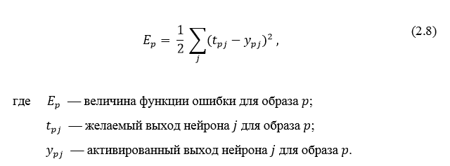
Неактивированное состояние каждого нейрона j для образа p записывается в виде взвешенной суммы по формуле 2.9:

Выход каждого нейрона j является значением активационной функции
 , которая переводит нейрон в активированное состояние. В качестве функции активации может использоваться любая непрерывно дифференцируемая монотонная функция. Активированное состояние нейрона вычисляется по формуле 2.10:

В качестве метода минимизации ошибки используется метод градиентного спуска, суть этого метода сводится к поиску минимума (или максимума) функции за счет движения вдоль вектора градиента. Для поиска минимума движение должно быть осуществляться в направлении антиградиента. Метод градиентного спуска в соответствии с рисунком 2.7.
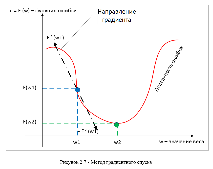
Градиент функции потери представляет из себя вектор частных производных, вычисляющийся по формуле 2.11:

Производную функции ошибки по конкретному образу можно записать по правилу цепочки, формула 2.12:
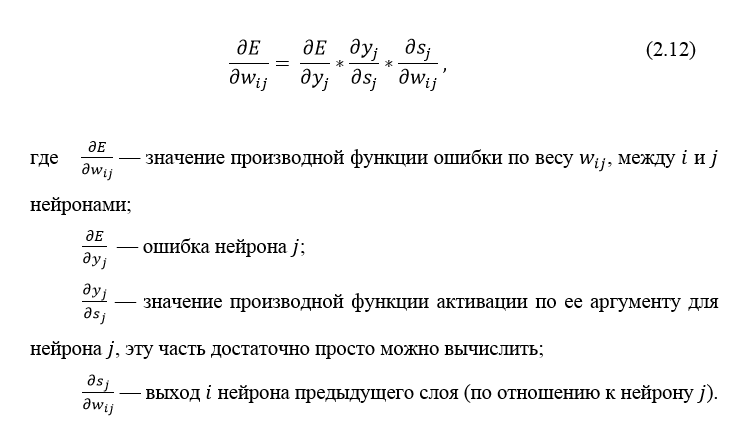
Ошибка нейрона  обычно записывается в виде символа ? (дельта). Для выходного слоя ошибка определена в явном виде, если взять производную от формулы 2.8, то получим t минус y, то есть разницу между желаемым и полученным выходом. Но как рассчитать ошибку для скрытых слоев? Для решения этой задачи, как раз и был придуман алгоритм обратного распространения ошибки. Суть его заключается в последовательном вычислении ошибок скрытых слоев с помощью значений ошибки выходного слоя, т.е. значения ошибки распространяются по сети в обратном направлении от выхода к входу.
Ошибка ? для скрытого слоя рассчитывается по формуле 2.13:

Алгоритм распространения ошибки сводится к следующим этапам:
- прямое распространение сигнала по сети, вычисления состояния нейронов;
- вычисление значения ошибки ? для выходного слоя;
- обратное распространение: последовательно от конца к началу для всех скрытых слоев вычисляем ? по формуле 2.13;
- обновление весов сети на вычисленную ранее ? ошибки.
Алгоритм обратного распространения ошибки в многослойном персептроне продемонстрирован ниже:
До этого момента были рассмотрены случаи распространения ошибки по слоям персептрона, то есть по выходному и скрытому, но помимо них, в сверточной нейросети имеются подвыборочный и сверточный.
Расчет ошибки на подвыборочном слое
Расчет ошибки на подвыборочном слое представляется в нескольких вариантах. Первый случай, когда подвыборочный слой находится перед полносвязным, тогда он имеет нейроны и связи такого же типа, как в полносвязном слое, соответственно вычисление ? ошибки ничем не отличается от вычисления ? скрытого слоя. Второй случай, когда подвыборочный слой находится перед сверточным, вычисление ? происходит путем обратной свертки. Для понимания обратно свертки, необходимо сперва понять обычную свертку и то, что скользящее окно по карте признаков (во время прямого распространения сигнала) можно интерпретировать, как обычный скрытый слой со связями между нейронами, но главное отличие — это то, что эти связи разделяемы, то есть одна связь с конкретным значением веса может быть у нескольких пар нейронов, а не только одной. Интерпретация операции свертки в привычном многослойном виде в соответствии с рисунком 2.8.
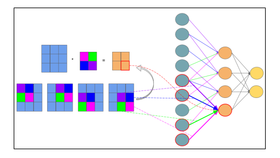
Рисунок 2.8 — Интерпретация операции свертки в многослойный вид, где связи с одинаковым цветом имеют один и тот же вес. Синим цветом обозначена подвыборочная карта, разноцветным – синаптическое ядро, оранжевым – получившаяся свертка
Теперь, когда операция свертки представлена в привычном многослойном виде, можно интуитивно понять, что вычисление дельт происходит таким же образом, как и в скрытом слое полносвязной сети. Соответственно имея вычисленные ранее дельты сверточного слоя можно вычислить дельты подвыборочного, в соответствии с рисунком 2.9.

Обратная свертка – это тот же самый способ вычисления дельт, только немного хитрым способом, заключающийся в повороте ядра на 180 градусов и скользящем процессе сканирования сверточной карты дельт с измененными краевыми эффектами. Простыми словами, нам необходимо взять ядро сверточной карты (следующего за подвыборочным слоем) повернуть его на 180 градусов и сделать обычную свертку по вычисленным ранее дельтам сверточной карты, но так чтобы окно сканирования выходило за пределы карты. Результат операции обратной свертки в соответствии с рисунком 2.10, цикл прохода обратной свертки в соответствии с рисунком 2.11.

Рисунок 2.10 — Результат операции обратной свертки

Рисунок 2.11 — Повернутое ядро на 180 градусов сканирует сверточную карту
Расчет ошибки на сверточном слое
Обычно впередиидущий слой после сверточного это подвыборочный, соответственно наша задача вычислить дельты текущего слоя (сверточного) за счет знаний о дельтах подвыборочного слоя. На самом деле дельта ошибка не вычисляется, а копируется. При прямом распространении сигнала нейроны подвыборочного слоя формировались за счет неперекрывающегося окна сканирования по сверточному слою, в процессе которого выбирались нейроны с максимальным значением, при обратном распространении, мы возвращаем дельту ошибки тому ранее выбранному максимальному нейрону, остальные же получают нулевую дельту ошибки.
Заключение
Представив операцию свертки в привычном многослойном виде (рисунок 2.8), можно интуитивно понять, что вычисление дельт происходит таким же образом, как и в скрытом слое полносвязной сети.
Источники
Алгоритм обратного распространения ошибки для сверточной нейронной сети
Обратное распространение ошибки в персептроне
Еще можно почитать в РГБ диссертацию Макаренко: АЛГОРИТМЫ И ПРОГРАММНАЯ СИСТЕМА КЛАССИФИКАЦИИ
Применение алгоритма обратного распространения ошибки — один из известных методов, используемых для глубокого обучения нейронных сетей прямого распространения (такие сети ещё называют многослойными персептронами). Этот метод относят к методу обучения с учителем, поэтому требуется задавать в обучающих примерах целевые значения. В этой статье мы рассмотрим, что собой представляет метод обратного распространения ошибки, как он реализуется, каковы его плюсы и минусы.
Сегодня нейронные сети прямого распространения используются для решения множества сложных задач. Если говорить об обучении нейронных сетей методом обратного распространения, то тут пользуются двумя проходами по всем слоям нейросети: прямым и обратным. При выполнении прямого прохода осуществляется подача входного вектора на входной слой сети, после чего происходит распространение по нейронной сети от слоя к слою. В итоге должна осуществляться генерация набора выходных сигналов — именно он, по сути, является реакцией нейронной сети на этот входной образ. При прямом проходе все синаптические веса нейросети фиксированы. При обратном проходе все синаптические веса настраиваются согласно правил коррекции ошибок, когда фактический выход нейронной сети вычитается из желаемого, что приводит к формированию сигнала ошибки. Такой сигнал в дальнейшем распространяется по сети, причём направление распространения обратно направлению синаптических связей. Именно поэтому соответствующий метод и называют алгоритмом с обратно распространённой ошибкой. Синаптические веса настраивают с целью наибольшего приближения выходного сигнала нейронной сети к желаемому.
Общее описание алгоритма обратного распространения ошибки
К примеру, нам надо обучить нейронную сеть по аналогии с той, что представлена на картинке ниже. Естественно, задачу следует выполнить, применяя алгоритм обратного распространения ошибки:
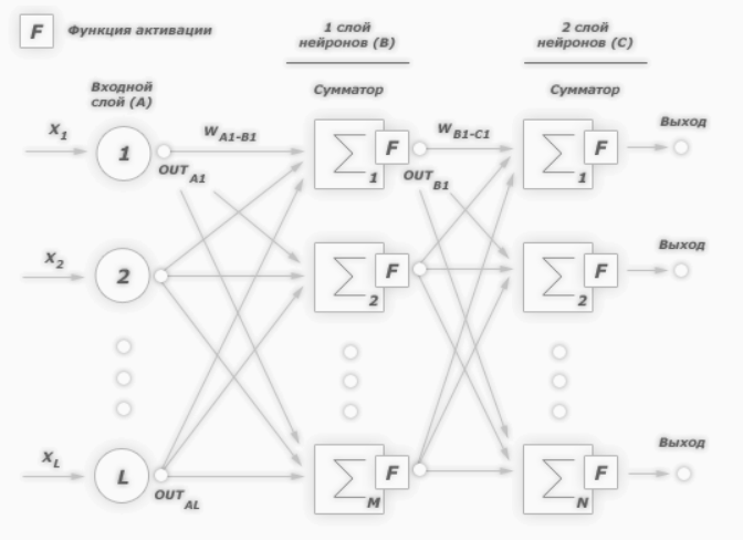
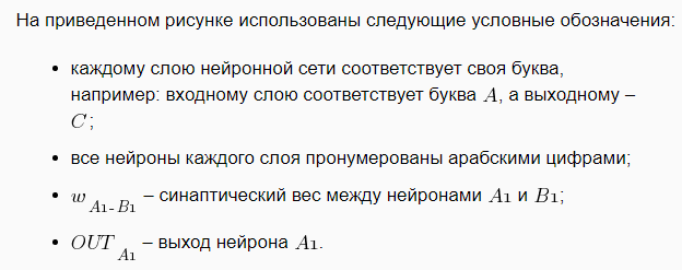
В многослойных персептронах в роли активационной функции обычно применяют сигмоидальную активационную функция, в нашем случае — логистическую. Формула:

Причём «альфа» здесь означает параметр наклона сигмоидальной функции. Меняя его, мы получаем возможность строить функции с разной крутизной.
Сигмоид может сужать диапазон изменения таким образом, чтобы значение OUT лежало между нулем и единицей. Нейронные многослойные сети характеризуются более высокой представляющей мощностью, если сравнивать их с однослойными, но это утверждение справедливо лишь в случае нелинейности. Нужную нелинейность и обеспечивает сжимающая функция. Но на практике существует много функций, которые можно использовать. Говоря о работе алгоритма обратного распространения ошибки, скажем, что для этого нужно лишь, чтобы функция была везде дифференцируема, а данному требованию как раз и удовлетворяет сигмоид. У него есть и дополнительное преимущество — автоматический контроль усиления. Если речь идёт о слабых сигналах (OUT близко к нулю), то кривая «вход-выход» характеризуется сильным наклоном, дающим большое усиление. При увеличении сигнала усиление падает. В результате большие сигналы будут восприниматься сетью без насыщения, а слабые сигналы будут проходить по сети без чрезмерного ослабления.
Цель обучения сети
Цель обучения нейросети при использовании алгоритма обратного распространения ошибки — это такая подстройка весов нейросети, которая позволит при приложении некоторого множества входов получить требуемое множество выходов нейронов (выходных нейронов). Можно назвать эти множества входов и выходов векторами. В процессе обучения предполагается, что для любого входного вектора существует целевой вектор, парный входному и задающий требуемый выход. Эту пару называют обучающей. Работая с нейросетями, мы обучаем их на многих парах.
Также можно сказать, что алгоритм использует стохастический градиентный спуск и продвигается в многомерном пространстве весов в направлении антиградиента, причём цель — это достижение минимума функции ошибки.
При практическом применении метода обучение продолжают не до максимально точной настройки нейросети на минимум функции ошибки, а пока не будет достигнуто довольно точное его приближение. С одной стороны, это даёт возможность уменьшить количество итераций обучения, с другой — избежать переобучения нейронной сети.
Пошаговая реализация метода обратного распространения ошибки
Необходимо выполнить следующие действия:
1. Инициализировать синаптические веса случайными маленькими значениями.
2. Выбрать из обучающего множества очередную обучающую пару; подать на вход сети входной вектор.
3. Выполнить вычисление выходных значений нейронной сети.
4. Посчитать разность между выходом нейросети и требуемым выходом (речь идёт о целевом векторе обучающей пары).
5. Скорректировать веса сети в целях минимизации ошибки.
6. Повторять для каждого вектора обучающего множества шаги 2-5, пока ошибка обучения нейронной сети на всём множестве не достигнет уровня, который является приемлемым.
Виды обучения сети по методу обратного распространения
Сегодня существует много модификаций алгоритма обратного распространения ошибки. Возможно обучение не «по шагам» (выходная ошибка вычисляется, веса корректируются на каждом примере), а «по эпохам» в offline-режиме (изменения весовых коэффициентов происходит после подачи на вход нейросети всех примеров обучающего множества, а ошибка обучения neural сети усредняется по всем примерам).
Обучение «по эпохам» более устойчиво к выбросам и аномальным значениям целевой переменной благодаря усреднению ошибки по многим примерам. Зато в данном случае увеличивается вероятность «застревания» в локальных минимумах. При обучении «по шагам» такая вероятность меньше, ведь применение отдельных примеров создаёт «шум», «выталкивающий» алгоритм обратного распространения из ям градиентного рельефа.
Преимущества и недостатки метода
К плюсам можно отнести простоту в реализации и устойчивость к выбросам и аномалиям в данных, и это основные преимущества. Но есть и минусы:
• неопределенно долгий процесс обучения;
• вероятность «паралича сети» (при больших значениях рабочая точка функции активации попадает в область насыщения сигмоиды, а производная величина приближается к 0, в результате чего коррекции весов почти не происходят, а процесс обучения «замирает»;
• алгоритм уязвим к попаданию в локальные минимумы функции ошибки.
Значение метода обратного распространения
Появление алгоритма стало знаковым событием и положительно отразилось на развитии нейросетей, ведь он реализует эффективный с точки зрения вычислительных процессов способ обучения многослойного персептрона. В то же самое время, было бы неправильным сказать, что алгоритм предлагает наиболее оптимальное решение всех потенциальных проблем. Зато он действительно развеял пессимизм относительно машинного обучения многослойных машин, который воцарился после публикации в 1969 году работы американского учёного с фамилией Минский.
Источники:
— «Алгоритм обратного распространения ошибки»;
— «Back propagation algorithm».