A false positive error or false positive (false alarm) is a result that indicates a given condition exists when it doesn’t.
You can get the number of false positives from the confusion matrix. For a binary classification problem, it is described as follows:
| Predicted = 0 | Predicted = 1 | Total | |
|---|---|---|---|
| Actual = 0 | True Negative (TN) | False Positive(FP) | N |
| Actual = 1 | False Negative (FN) | True Positive (TP) | P |
| Total | N * | P * |
In statistical hypothesis testing, the false positive rate is equal to the significance level, (alpha), and (1 — alpha) is defined as the specificity of the test. Complementarily, the false negative rate is given by (beta).
The different measures for classification are:
| Name | Definition | Synonyms |
|---|---|---|
| False positive rate ((alpha)) | FP/N | Type I error, 1- specificity |
| True Positive rate ((1-beta)) | TP/P | 1 — Type II error, power, sensitivity, recall |
| Positive prediction value | TP/P* | Precision |
| Negative prediction value | TN/N* | |
| Overall accuracy | (TN + TP)/N | |
| Overall error rate | (FP + FN)/N |
Also, note that F-score is the harmonic mean of precision and recall.
[text{F1 score} = frac{2 * text{precision} * text{recall}}{text{precision} + text{recall}}]
For example, in cancer detection, sensitivity and specificity are the following:
- Sensitivity: Of all the people with cancer, how many were correctly diagnosed?
- Specificity: Of all the people without cancer, how many were correctly diagnosed?
And precision and recall are the following:
- Recall: Of all the people who have cancer, how many did we diagnose as having cancer?
- Precision: Of all the people we diagnosed with cancer, how many actually had cancer?
Often, we want to make binary prediction e.g. in predicting the quality of care of the patient in the hospital, whether the patient receive poor care or good care? We can do this using a threshold value (t).
- if (P(poor care = 1) geq t), predict poor quality
- if (P(poor care = 1 < t), predict good quality
Now, the question arises, what value of (t) we should consider.
- if (t) is large, the model will predict poor care rarely hence detect patients receiving the worst care.
- if (t) is small, the model will predict good care rarely hence detect all patients receiving poor care.
i.e.
- A model with a higher threshold will have a lower sensitivity and a higher specificity.
- A model with a lower threshold will have a higher sensitivity and a lower specificity.
Thus, the answer to the above question depends on what problem you are trying to solve. With no preference between the errors, we normally select (t = 0.5).
Area Under the ROC Curve gives the AUC score of a model.
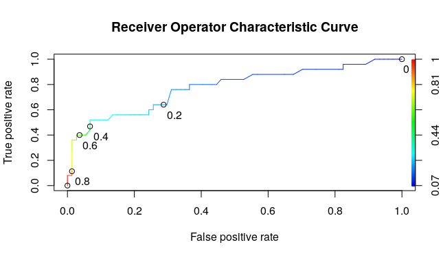
- The threshold of 1 means that the model will not catch any poor care cases, or have sensitivity of 0 but it’ll correctly label all the good care cases, meaning that you have a false positive rate of 0.
- The threshold of 0 means that the model will catch all of the poor care cases or have a sensitivity of 1, but it’ll label all of the good care cases as poor care cases too, meaning that you’ll have a false positive rate of 1.
Below is xkcd comic regarding the wrong interpretation of p-value and false positives.

Explanation of above comic on explain xkcd wiki.
References:
- An Introduction to Statistical Learning
- False positives and false negatives — Wikipedia
- Sensitivity and specificity — Wikipedia
- Precision and recall — Wikipedia
This page is open source. Improve its content!
-
1
error rate
Англо-русский словарь нормативно-технической терминологии > error rate
-
2
error rate
heart rate — частота пульса, частота сердечных сокращений
English-Russian big polytechnic dictionary > error rate
-
3
error rate
частота [появления] ошибок
1) параметр, характеризующий качество канала связи
2) число ошибок на тысячу строк исходного текста программы.
The error rate does not remain constant but increases with the size of the programs. — Частота появления ошибок не является величиной постоянной, а увеличивается по мере роста объёма программы KLOC
Англо-русский толковый словарь терминов и сокращений по ВТ, Интернету и программированию. > error rate
-
4
error rate
коэффициент ошибок; частота ошибок
English-Russian base dictionary > error rate
-
5
error rate
English-Russian dictionary of Information technology > error rate
-
6
error rate
Большой англо-русский и русско-английский словарь > error rate
-
7
error rate
Англо-русский словарь технических терминов > error rate
-
8
error rate
Англо-русский словарь нефтегазовой промышленности > error rate
-
9
error rate
9) SAP.тех. предрасположенность к возникновению ошибок
Универсальный англо-русский словарь > error rate
-
10
error rate
Англо-русский экономический словарь > error rate
-
11
error rate
Англо-русский словарь по компьютерной безопасности > error rate
-
12
error rate
English-Russian electronics dictionary > error rate
-
13
error rate
The New English-Russian Dictionary of Radio-electronics > error rate
-
14
error rate
коэффициент ошибок; частота ошибок
English-Russian dictionary of computer science and programming > error rate
-
15
error rate
Англо-русский словарь по полиграфии и издательскому делу > error rate
-
16
error rate
Англо-русский словарь по авиации > error rate
-
17
error rate
English-Russian dictionary of modern telecommunications > error rate
-
18
error rate
English-Russian dictionary of telecommunications and their abbreviations > error rate
-
19
error rate
English-Russian dictionary of terms that are used in computer games > error rate
-
20
error rate
частота появления ошибок; частота ошибок
English-Russian dictionary of technical terms > error rate
Страницы
- Следующая →
- 1
- 2
- 3
- 4
- 5
- 6
- 7
См. также в других словарях:
-
Error Rate — [engl.], Fehlerrate … Universal-Lexikon
-
error rate — In communications, the ratio between the number of bits received incorrectly and the total number of bits in the transmission, also known as bit error rate (BER). Some methods for determining error rate use larger or logical units, such as… … Dictionary of networking
-
error rate — klaidų dažnis statusas T sritis automatika atitikmenys: angl. error rate vok. Fehlerhäufigkeit, f; Fehlerrate, f rus. частота ошибок, f pranc. fréquence des erreurs, f … Automatikos terminų žodynas
-
error rate — klaidų intensyvumas statusas T sritis automatika atitikmenys: angl. error rate vok. Fehlerrate, f rus. интенсивность потока ошибок, f pranc. débit d erreur, m … Automatikos terminų žodynas
-
error rate — A measure of data integrity, expressed as the fraction of flawed bits; often expressed as a negative power of 10 as in 10 (a rate of one error in every one million bits) … IT glossary of terms, acronyms and abbreviations
-
Error rate — Частота (появления) ошибок … Краткий толковый словарь по полиграфии
-
error rate — n. ratio of incorrect assignments to categories or classes of a classification (Archaeology) … English contemporary dictionary
-
error rate — Number of faulty products expressed as a percentage of total output … American business jargon
-
error rate — / erə reɪt/ noun the number of mistakes per thousand entries or per page … Marketing dictionary in english
-
error rate — / erə reɪt/ noun the number of mistakes per thousand entries or per page … Dictionary of banking and finance
-
Technique for Human Error Rate Prediction — (THERP) is a technique used in the field of Human reliability Assessment (HRA), for the purposes of evaluating the probability of a human error occurring throughout the completion of a specific task. From such analyses measures can then be taken… … Wikipedia
The EER refers to that point in a DET (Detection Error Tradeoff) curve where the FAR (False Acceptance rate) equals the FRR (False Rejection Rate).
From: Advances in Ubiquitous Computing, 2020
Replay attack detection using excitation source and system features
Madhusudan Singh, Debadatta Pati, in Advances in Ubiquitous Computing, 2020
2.4.3.1 Equal error rate and detection error tradeoff
The SV performance is generally shown by a detection error tradeoff (DET) curve and measured in terms of EER, where the false rejection rate (FRR) and false acceptance rate (FAR) are equal [49]. In false rejection, a genuine is classified as an impostor while in false acceptance, an impostor is accepted as a genuine speaker. Under a replay spoofing scenario, the replay attackers usually aim at specified (target) speakers and thereby increase the FAR of the system. Thus, under replay attacks, the FAR is a more relevant measuring parameter for evaluating the system performance. Accordingly, we have used two metrics to evaluate the system performance under both the baseline and spoofing test conditions: zero-effort false acceptance rate (ZFAR) and replay attack false acceptance rate (RFAR). ZFAR and RFAR are related to zero-effort impostor trials and replay trials, respectively.
The baseline ZFAR or equivalently the EER performance is computed by pooling all genuine and zero-effort impostor trials together. The RFAR performance is computed using the replay trials only, under replay attacks. The computation of RFAR is based on the fixed decision threshold (at EER point) of the baseline system, as shown in Fig. 2.5. As the same baseline ASV system is used for both ZFAR and RFAR computation, the difference RFAR-ZFAR directly indicates system vulnerability to replay attacks [3]. In a positive sense, it represents ASV systems’ capability to resist spoof attacks. A smaller value of RFAR-ZFAR indicates better replay detection accuracy. For a foolproof spoof-resistant (RFAR = 0) ASV system, the RFAR-ZFAR will approach to (-ZFAR). Moreover, since the same ASV system is used for both baseline and spoofing tests, the scores and decisions for all genuine trials will remain unaffected. Consequently, the FRR will remain constant, under both test conditions. Altogether, ZFAR, RFAR, and their difference RFAR-ZFAR can be used as evaluation metrics to compare the different ASV systems’ performance under a replay spoofing scenario.

Fig. 2.5. Synthetic example showing computation of ZFAR and RFAR using a decision threshold fixed at EER point (P) of the baseline system.
Read full chapter
URL:
https://www.sciencedirect.com/science/article/pii/B9780128168011000025
The use of WSN (wireless sensor network) in the surveillance of endangered bird species
Amira Boulmaiz, … Djemil Messadeg, in Advances in Ubiquitous Computing, 2020
9.9.2.1 Segmentation and recognition performance
To examine the performance and efficiency of the proposed segmentation method, namely TRD, we took the sound of the Ferruginous Duck with a duration just over 6 s with a sampling rate of 44.1 kHz, which gives a total number of samples of 265,250. Its time domain and spectrogram graphs are shown in Fig. 9.17A. By adding an environment noise, which leads to a SNR = 10 dB, we can get the time domain and spectrogram graphs of noisy sound shown in Fig. 9.17B. Fig. 9.17C represents the time domain graph and spectrogram of the noisy bird sound after applying the proposed tonal region detector (TRD). The samples are reducing from 265,250 down to 44,109, which represent approximately one-quarter of the total number of samples.

Fig. 9.17. The time domain graph of selected Ferruginous Duck sound in the left and his spectrogram in the right (A) in clean condition, (B) perturbed by environment noise at SNR = 10 dB, and (C) after applying the tonal region detector (TRD).
The recognition performance for different front-end/normalization setups found per each feature extraction strategy (GTECC, MFCC, PMVDR, PNCC, and MWSCC) is given in Fig. 9.18. The results are reported in terms of EER (equal error rates). The EER refers to that point in a DET (Detection Error Tradeoff) curve where the FAR (False Acceptance rate) equals the FRR (False Rejection Rate). A perfect scoring model would yield an EER of zero, so a lower EER value indicates a better performance.

Fig. 9.18. Performance comparison of alternative popular features considered in this study against GTECC in terms of EERs (%) for different values of SNR: (A) SNR = 50 dB, (B) SNR varies from 30 to 0 dB, (C) SNR varies from 0 to − 10 dB, and (D) the average values.
The training sounds data were corrupted by an additive white Gaussian noise (AWGN) with a SNR equal to 50 dB. However, the testing data were corrupted by an AWGN with a SNR that varies from − 10 to 30 dB in 5-dB steps, in order to simulate the real-world complex noisy environments. From Fig. 9.18, we can see that the proposed GTECC front-end is almost in all cases (whether in clean or noisy conditions) the most efficient in terms of EER, with or without application of a method of normalization. Moreover, GTECC postprocessed by Quantile-based cepstral dynamics normalization (GTECC-QCN) gives an average EER equal to 10.18%, which is the lowest EER compared to the other studied methods, followed by MWSCC-QCN with an average EER of 11.61% and PNCC-QCN with an average EER equal to 12.87%, then MFCC-QCN with an average EER equal to 13.78%, then PMCC-QCN with an average EER equal to 14.11%, and finally PMVDR-QCN with an average EER equal to 14.91%.
Let us consider now the performance of normalization methods used in our study for the reduction of noise in the detected segments as tonal regions in the sound of a bird. From Fig. 9.18, we can observe that spectral subtraction (SS) is less effective for reducing white Gaussian noise, especially with a SNR < 0 dB. Normalizations CMVN and CGN have relatively similar results on the Gaussian white noise with a significantly superior performance of the normalization CGN, when applied to PMVDR, in the presence of AWGN with a SNR between 0 and − 10 dB. Finally, QCN has the best performance when applied to the six methods of characterization studied namely GTECC, MFCC, PMVDR, PMCC, PNCC, and MWSCC.
Read full chapter
URL:
https://www.sciencedirect.com/science/article/pii/B9780128168011000098
Generative adversarial network for video anomaly detection
Thittaporn Ganokratanaa, Supavadee Aramvith, in Generative Adversarial Networks for Image-to-Image Translation, 2021
16.4.4 Performance of DSTN
We evaluate the proposed DSTN regarding accuracy and time complexity aspects. The ROC curve is used to illustrate the performance of anomaly detection at the frame level and the pixel level and analyze the experimental results with other state-of-the-art works. Additionally, the AUC and the EER are evaluated as the criteria for determining the results.
The performance of DSTN is first evaluated on the UCSD dataset, consisting of 10 and 12 videos for the UCSD Ped1 and the UCSD Ped2 with the pixel-level ground truth, by using both frame-level and pixel-level protocols. In the first stage of DSTN, patch extraction is implemented to provide the appearance features of the foreground object and its motion regarding the vector changes in each patch. The patches are extracted independently from each original image with a size of 238 × 158 pixels (UCSD Ped1) and 360 × 240 pixels (UCSD Ped2) to apply it with (w/4) × h × cp. As a result, we obtain 22 k patches from the UCSD Ped1 and 13.6 k patches from the UCSD Ped2. Then, to feed into the spatiotemporal translation model, we resize all patches to the 256 × 256 default size in both training and testing time.
During training, the input of G (the concatenation of f and fBR patches) and target data (the generated dense optical flow OFgen) are set to the same size as the default resolution of 256 × 256 pixels. The encoding and decoding modules in G are implemented differently. As in the encoder network, the image resolution is encoded from 256 → 128 → 64 → 32 → 16 → 8 → 4 → 2 → 1 to obtain the latent space representing the spatial image in one-dimensional data space. CNN effectively employs this downscale with kernels of 3 × 3 and stride s = 2. Additionally, the number of neurons corresponding to the image resolution in En is introduced in each layer from 6 → 64 → 128 → 256 → 512 → 512 → 512 → 512 → 512. In contrast, De decodes the latent space to reach the target data (the temporal representation of OFgen) with a size of 256 × 256 pixels using the same structure as En. The dropout is employed in De as noise z to remove the neuron connections using probability p = 0.5, resulting in the prevention of overfitting on the training samples. Since D needs to fluctuate G to correct the classification between real and fake images at training time, PatchGAN is then applied by inputting a patch size of 64 × 64 pixels to output the probability of class label for the object. The PatchGAN architecture is constructed from 64 → 32 → 16 → 8 → 4 → 2 → 1, which is then flattened to 512 neurons and plugged in with Fully Connection (FC) and Softmax layers. The use of PatchGAN benefits the model in terms of time complexity. This is probably because there are fewer parameters to learn on the partial image, making the model less complex and can achieve good running time for the training process. In the aspect of testing, G is specifically employed to reconstruct OFgen in order to analyze the real motion information OFfus. The image resolution for testing and training are set to the same resolution for all datasets.
The quantitative performance of DSTN is presented in Table 16.1 where we consider the DSTN with various state-of-the-art works, e.g., AMDN [15], GMM-FCN [12], Convolutional AE [14], and future frame prediction [21]. From Table 16.1 it can be observed that the DSTN overcomes most of the methods in both frame-level and pixel-level criteria since we achieve higher AUC and lower EER on the UCSD Dataset. Moreover, we show the qualitative performance of DSTN using the standard evaluation for anomaly detection research known as the ROC curves, where we vary a threshold from 0 to 1 to plot the curve of TPR against FPR. The qualitative performance of DSTN is compared with other approaches in both frame-level evaluation (see Fig. 16.20A) and pixel-level evaluation (see Fig. 16.20B) on the UCSD Ped1 and at the frame-level evaluation on the UCSD Ped2 as presented in Figs. 16.20 and 16.21, respectively. Following Figs. 16.20 and 16.21, the DSTN (circle) shows the strongest growth curve on TPR and overcomes all the competing methods in the frame and pixel level. This means that the DSTN is a reliable and effective method to be able to detect and localize the anomalies with high precision.
Table 16.1. EER and AUC comparison of DSTN with other methods on UCSD Dataset [26].
| Method | Ped1 (frame level) | Ped1 (pixel level) | Ped2 (frame level) | Ped2 (pixel level) | ||||
|---|---|---|---|---|---|---|---|---|
| EER | AUC | EER | AUC | EER | AUC | EER | AUC | |
| MPPCA | 40% | 59.0% | 81% | 20.5% | 30% | 69.3% | – | – |
| Social Force (SF) | 31% | 67.5% | 79% | 19.7% | 42% | 55.6% | 80% | – |
| SF + MPPCA | 32% | 68.8% | 71% | 21.3% | 36% | 61.3% | 72% | – |
| Sparse Reconstruction | 19% | – | 54% | 45.3% | – | – | – | – |
| MDT | 25% | 81.8% | 58% | 44.1% | 25% | 82.9% | 54% | – |
| Detection at 150fps | 15% | 91.8% | 43% | 63.8% | – | – | – | – |
| SR + VAE | 16% | 90.2% | 41.6% | 64.1% | 18% | 89.1% | – | – |
| AMDN (double fusion) | 16% | 92.1% | 40.1% | 67.2% | 17% | 90.8% | – | – |
| GMM | 15.1% | 92.5% | 35.1% | 69.9% | – | – | – | – |
| Plug-and-Play CNN | 8% | 95.7% | 40.8% | 64.5% | 18% | 88.4% | – | – |
| GANs | 8% | 97.4% | 35% | 70.3% | 14% | 93.5% | – | – |
| GMM-FCN | 11.3% | 94.9% | 36.3% | 71.4% | 12.6% | 92.2% | 19.2% | 78.2% |
| Convolutional AE | 27.9% | 81% | – | – | 21.7% | 90% | – | – |
| Liu et al. | 23.5% | 83.1% | – | 33.4% | 12% | 95.4% | – | 40.6% |
| Adversarial discriminator | 7% | 96.8% | 34% | 70.8% | 11% | 95.5% | – | – |
| AnomalyNet | 25.2% | 83.5% | – | 45.2% | 10.3% | 94.9% | – | 52.8% |
| DSTN (proposed method) | 5.2% | 98.5% | 27.3% | 77.4% | 9.4% | 95.5% | 21.8% | 83.1% |


Fig. 16.20. ROC Comparison of DSTN with other methods on UCSD Ped1 dataset: (A) frame-level evaluation and (B) pixel-level evaluation [26].

Fig. 16.21. ROC Comparison of DSTN with other methods on UCSD Ped2 dataset at frame-level evaluation [26].
Examples of the experimental results of DSTN on the UCSD Ped 1 and Ped 2 dataset are illustrated in Fig. 16.22 to extensively present its performance in detecting and localizing anomalies in the scene. According to Fig. 16.22, the proposed DSTN is able to detect and locate various types of abnormalities effectively with each object, e.g., (a) a wheelchair, (b) a vehicle, (c) a skateboard, and (d) a bicycle, or even more than one anomaly in the same scene, e.g., (e) bicycles, (f) a vehicle and a bicycle, and (g) a bicycle and a skateboard. However, we face the false positive problems in Fig. 16.22H a bicycle and a skateboard, where the walking person (normal event) is detected as an anomaly. Even the bicycle and the skateboard are correctly detected as anomalies in Fig. 16.22H, the false detection on the walking person makes this frame wrong anyway. The false positive anomaly detection is probably caused by a similar speed of walking to cycling in the scene.


Fig. 16.22. Examples of DSTN performance in detecting on localizing anomalies on UCSD Ped1 and Ped2 dataset: (A) a wheelchair, (B) a vehicle, (C) a skateboard, (D) a bicycle, (E) bicycles, (F) a vehicle and a bicycle, (G) a bicycle and a skateboard, and (H) a bicycle and a skateboard [26].
For the UMN dataset, the performance of DSTN is evaluated using the same settings as training parameters and network configuration on the UCSD pedestrian dataset. Table 16.2 indicates the AUC performance comparison of the DSTN with various competing works such as GANs [20], adversarial discriminator [22], AnomalyNet [23], and so on. Table 16.2 shows that the proposed DSTN achieves the best AUC results the same as Ref. [23], which outperforms all other methods. Noticeably, most of the competing methods can achieve high AUC on the UMN dataset. This is because the UMN dataset has less complexity regarding its abnormal patterns than the UCSD pedestrian and the Avenue datasets. Fig. 16.23 shows the performance of DSTN in detecting and localizing anomalies in different scenarios on the UMN dataset, including (d) an indoor and outdoors in (a), (b), and (c), where we can detect most of the individual objects in the crowded scene.
Table 16.2. AUC comparison of DSTN with other methods on UMN dataset [26].
| Method | AUC |
|---|---|
| Optical-flow | 0.84 |
| SFM | 0.96 |
| Sparse reconstruction | 0.976 |
| Commotion | 0.988 |
| Plug-and-play CNN | 0.988 |
| GANs | 0.99 |
| Adversarial discriminator | 0.99 |
| Anomalynet | 0.996 |
| DSTN (proposed method) | 0.996 |

Fig. 16.23. Examples of DSTN performance in detecting on localizing anomalies on UMN dataset, where (A), (B), and (D) contain running activity outdoors while (C) is in an indoor [26].
Apart from evaluating DSTN on the UCSD and the UMN datasets, we also assess our performance on the challenging CUHK Avenue dataset with the same parameter and configuration settings as the UCSD and the UMN datasets. Table 16.3 presents the performance comparison in terms of EER and AUC of the DSTN with other competing works [6, 12, 14, 21, 23] in which the proposed DSTN surpasses all state-of-the-art works for both protocols. We show examples of the DSTN performance in detecting and localizing various types of anomalies, e.g., (a) jumping, (b) throwing papers, (c) falling papers, and (d) grabbing a bag, on the CUHK Avenue dataset in Fig. 16.24 The DSTN can effectively detect and localize anomalies in this dataset, even in Fig. 16.24D, which contains only small movements for abnormal events (only the human head and the fallen bag are slightly moving).
Table 16.3. EER and AUC comparison of DSTN with other methods on CUHK Avenue dataset [26].
| Method | EER | AUC |
|---|---|---|
| Convolutional AE | 25.1% | 70.2% |
| Detection at 150 FPS | – | 80.9% |
| GMM-FCN | 22.7% | 83.4% |
| Liu et al. | – | 85.1% |
| Anomalynet | 22% | 86.1% |
| DSTN (proposed method) | 20.2% | 87.9% |

Fig. 16.24. Examples of DSTN performance in detecting on localizing anomalies on CUHK Avenue dataset: (A) jumping, (B) throwing papers, (C) falling papers, and (D) grabbing a bag [26].
To indicate the significance of our performance for real-time use, we then compare the running time of DSTN during testing in seconds per frame as shown in Table 16.4 with other competing methods [3–6, 15] following the environment and the computational time from Ref. [15].
Table 16.4. Running time comparison on testing measurement (seconds per frame).
| Method | CPU (GHz) | GPU | Memory (GB) | Running time | |||
|---|---|---|---|---|---|---|---|
| Ped1 | Ped2 | UMN | Avenue | ||||
| Sparse Reconstruction | 2.6 | – | 2.0 | 3.8 | – | 0.8 | – |
| Detection at 150 fps | 3.4 | – | 8.0 | 0.007 | – | – | 0.007 |
| MDT | 3.9 | – | 2.0 | 17 | 23 | – | – |
| Li et al. | 2.8 | – | 2.0 | 0.65 | 0.80 | – | – |
| AMDN (double fusion) | 2.1 | Nvidia Quadro K4000 | 32 | 5.2 | – | – | – |
| DSTN (proposed method) | 2.8 | – | 24 | 0.315 | 0.319 | 0.318 | 0.334 |
Regarding Table 16.4, we achieve a lower running time than most of the competing methods except for Ref. [6]. This is because the architecture of DSTN relies on the framework of the deep learning model using multiple layers of the convolutional neural network, which is more complex than Ref. [6] that uses the learning of a sparse dictionary and provides fewer connections. However, according to the experimental results in Tables 16.1 and 16.3, our proposed DSTN significantly provides higher AUC and lower EER with respect to the frame and the pixel level on the CUHK Avenue and the UCSD pedestrian datasets than Ref. [6]. Regarding the running time, the proposed method runs 3.17 fps for the UCSD Ped1 dataset, 3.15 fps for the UCSD Ped2 dataset, 3.15 fps for the UMN dataset, and 3 fps for the CUHK Avenue dataset. In every respect, we provide the performance comparison of the proposed DSTN with other competing works [3–6, 15] to show our performance in regard to the frame-level AUC and the running time in seconds per frame for the UCSD Ped1 and Ped2 dataset as presented in Figs. 16.25 and 16.26, respectively.

Fig. 16.25. Frame-level AUC comparison and running time on UCSD Ped1 dataset.

Fig. 16.26. Frame-level AUC comparison and running time on UCSD Ped2 dataset.
Considering Figs. 16.25 and 16.26, our proposed method achieves the best results regarding the AUC and running time aspects. In this way, we can conclude that our DSTN surpasses other state-of-the-art approaches since we reach the highest AUC values at the frame level anomaly detection and the pixel level localization and given the good computational time for real-world applications.
Read full chapter
URL:
https://www.sciencedirect.com/science/article/pii/B9780128235195000117
Cognitive radio evolution
Joseph MitolaIII, in Cognitive Radio Communications and Networks, 2010
20.4.2 Human Language and Machine Translation
Computer processing of human language includes both real-time speech recognition and high-performance text processing as well as machine translation. During the evolution period of Table 20.1, CRs may perceive spoken and written human language (HL) with sufficient reliability to detect, characterize, and respond appropriately to stereotypical situations, unburdening the user from the counterproductive tedium of identifying the situation for the radio. Machine translation in the cell phone may assist global travelers with greetings, hailing a taxi, understanding directions to the restaurant, and the like. Such information prosthetics may augment today’s native language facilities. With ubiquity of coverage behind it, CRA evolves toward more accurately characterizing the user’s information needs, such as via speech recognition and synthesis to interact with wearable wireless medical instruments, opening new dimensions of QoI.
Computer Speech
Computer speech technology offers opportunities for machine perception of content in well-structured audio channels such as 800 directory assistance. Although deployed with all Windows XPTM laptops, speech recognition does not appear to be in wide use for interaction with personal electronics or machine dictation. However, the technology now is mature enough to transcribe carefully spoken speech in benign acoustic environments such as a (quiet) home office, with 3–10% raw word error rates, reduced in structured utterances such as dictation to less than 2%. In situations where the speech is emotional, diffluent, heavily accented, or focused on a rare topic, the word error rates increase to about 25%, but even with these high word error rates topic spotting for geographical topics can yield 14.7% precision, improved by an order of magnitude during the past five years [767].
Speaker identification technology [768] has equal error rates (equal probability of false dismissal and false alarm) of <10% for relatively small collections of speakers (<100). Such algorithms are influenced (usually corrupted) by acoustic backgrounds that distort the speaker models. Speaker recognition may be termed a soft biometric since it could be used to estimate a degree of belief that the current speaker is the usual user of the CR to align user profiles. Such speaker modeling could contribute to multifactor biometrics to deter the theft of personal information from wireless devices.
Text Understanding
Business intelligence markets are deploying text understanding technology that typically focuses on the quantitative assessment of the metrics of text documents, such as to assess and predict the performance of a business organization. Quantitative analysis of databases and spreadsheets often do not clearly establish the causal relationships needed for related business decision making. Causal cues typically are evident in the unstructured text of business documents like customer contact reports, but the extraction of those relationships historically has been excessively labor intensive. Therefore, businesses, law enforcement, and government organizations are employing text analysis to enhance their use of unstructured text for business intelligence [769], with rapidly growing markets. These products mix word sense disambiguation, named entity detection, and sentence structure analysis with business rules for more accurate business metrics than is practicable using purely statistical text mining approaches on relatively small text corpora. Google depends on the laws of very large numbers, but medium to large businesses may generate only hundreds to thousands of customer contact reports in the time interval of interest. For example, IBM’s unstructured information management architecture (UIMA) [770] text analysis analyzes small samples of text in ways potentially relevant to cognitive radio architecture evolution such as product defect detection.
In addition, Google’s recent release of the Android open handset alliance software [771] suggests a mix of statistical machine learning with at least shallow analysis of user input (e.g., for intent in the Android tool box). Google has become a popular benchmark for text processing. For example, a query tool based on ALICE (artificial linguistic Internet computer entity) is reported to improve on Google by 22% (increasing proportion of finding answers from 46% to 68%) in interactive question answering with a small sample of 21 users. Of the half of users expressing a preference, 40% preferred the ALICE-based tool (FAQchat) [772]. The commercial successful text retrieval market led by Google is stimulating research increasingly relevant to cognitive radio architecture evolution. For example, unstructured comments in wireless network service and maintenance records can yield early insight into product and service issues before they become widespread. This can lead to quicker issue resolution and lower aftermarket service and recall costs. Cognitive wireless networks (CWNs) might analyze their own maintenance records to discover operations, administration, and maintenance issues with less human oversight [773], enhancing the cost-effectiveness of cognitive devices and infrastructure compared to conventionally maintained wireless products and networks. This might entail a combination of text processing and functional description languages (FDL) such as the E3 FDL [749, 774].
The global mobility of the foundation era of Table 20.1 spurred the creation of world-phones such as GSM mobile phones that work nearly everywhere. During the evolution era, text analysis, real-time speech translation [775], text translation [776], image translation [777], and automatic identification of objects in images [778] will propel CRA evolution toward the higher layers of the protocol stack, ultimately with the user (from preferences to personal data) as the eighth layer. For example, if a future cognitive PDA knows from its most recent GPS coordinates that it is near the location of a new user’s home address and recognizes light levels consistent indoors as well as a desk and chair, then it could enable Bluetooth to check for a home computer, printer, and other peripherals. Detecting such peripherals, it could ask the user to approve sharing of data with these peripherals so that the PDA could automatically acquire information needed to assist the user, such as the user’s address book. The user could either provide permission or explain, for example, “You are my daughter’s new PDA, so you don’t need my address book. But it is OK to get hers. Her name is Barbara.” Objects prototypical of work and leisure events such as golf clubs could stimulate proactive behavior to tailor the PDA to the user, such as wallpaper of the great Scottish golf courses.
Read full chapter
URL:
https://www.sciencedirect.com/science/article/pii/B9780123747150000204
Human Factors
Luis M. Bergasa, … Joshua Puerta, in Intelligent Vehicles, 2018
9.1.5.3 General Observations
We begin by pointing out that one main drawback to perform a fair comparison between results obtained with different methods is the lack of a common database. Results obtained with one database could be biased by data collected and, maybe, the specific characteristics of driver environment. Performance of the algorithms depends also on data collected, CAN bus data are widely recorded, but other acquired signals could lead to achieving the best results, independently of the selected method.
A second observation is that most research papers only show the correct recognition rates to measure the goodness of the algorithm. Correct recognition performance is a vague indicator of algorithm actuation. For example, if our test set is formed by 95% samples which are labeled “normal driving” behavior and 5% samples with “aggressive driving,” a system with a constant output of “normal driving” will achieve 95% correct recognition. Even when this system is impossible to use, performance is in the state-of-the-art rates. More useful indicators to measure the performance of the algorithms are precision and recall. Precision is the fraction of retrieved instances that are relevant, let’s say “how useful the search results are,” while recall is the fraction of relevant instances that are retrieved, in other words, is “how complete the results are.” A single measure that combines both quantities is the traditional F-measure. The use of both indicators, together with F factor is highly recommended and encouraged. Other similar rates that better describe recognition performance are the false acceptance rate and false rejection rates, that can be combined to define Receiver operating characteristic (ROC) or detection error tradeoff (DET) curves. To represent recognition rate with a single quantity obtained from ROC curves, Equal Error Rate (EER) is widely used.
A third observation is that some systems increase the number of parameters when the input vector increases (e.g., adding more signals). In this case, the system may produce undesirable results. Trying to adjust one parameter may lead to an unpredictable result for other input data. Also, having more parameters to adjust requires more data in the training set, just to guarantee that enough samples are provided to the algorithm (and usually, input data are not so easy to obtain). If the training database is small, the algorithm could try to be overfitted to this training set with reduced generalization power.
A fourth observation is that the training set should be rich enough to cover a high spectrum of situations. Training with data obtained in very similar environments and testing with data obtained in other situations may lead to tricky results. Factors that have to be considered in experiment definition should include the number of drivers and experience of these drivers, drivers familiar or not with the scenario or the simulator; drivers with experience in the specific vehicle may obtain better results than novice ones.
A fifth observation is related to information extraction and feature definition. During the experimental phase a usual tradeoff should be achieved between the number of possible input signals and the cost of these signals. Since experimental data recording is expensive (drivers’ recruitment, simulator hours, vehicle consumption), a common criteria is to record “everything.” Once recorded, an initial information extraction procedure is suggested since maybe some variables could be correlated or could be combined without losing generality (but reducing processing time). In this initial procedure it is also advisable to estimate noisy signals that can be filtered or noise reduction procedure for signals that may require it.
A sixth observation is that the precise definition of classes is a complex task. Even simple classes like aggressive, calm, and normal driving have different definitions in research. Calm driving could mean optimal driving (in the sense of fuel consumption for example) or the driving condition that is more repeated or achieved in the training set. As a reference signal or indicator of driving behavior, fuel or energy consumption has been widely adopted. When this is not possible, experts in the field have been considered (e.g., in traffic safety) or the researcher directly evaluates the performance. Experts or external evaluation are preferred to avoid bias based on a priori knowledge of experiments.
A seventh observation notes that the acquisition of labeled data for a supervised driving learning process can be a costly and time-consuming task that requires the training of external evaluators. For naturalistic driving, where the driver voluntarily decides which tasks to perform at all times, the labeling process can become infeasible. However, data without known distraction states (unlabeled data) can be collected in an inexpensive way (e.g., from driver’s naturalistic driving records). In order to make use of these low cost data, semisupervised learning is proposed for model construction, due to its capability of extracting useful information from both labeled and unlabeled training data. Liu et al. (2016) investigate the benefit of semisupervised machine learning where unlabeled training data can be utilized in addition to labeled training data.
The last observation is related to implementation issues. Using onboard embedded hardware in the vehicle or smartphones as a recording and processing platform is now the state-of-the-art technology. They have enough recording space, processing power, and enough sensor devices at a very reasonable cost. They can be placed in any car to obtain naturalistic driving data using huge numbers of drivers and vehicle types. In the next years, new emergent techniques related to big data, deep learning, and data analytics will take advantage of these systems to improve intelligent vehicles’ capabilities.
Read full chapter
URL:
https://www.sciencedirect.com/science/article/pii/B9780128128008000096
Biometric Authentication to Access Controlled Areas Through Eye Tracking
Virginio Cantoni, … Haochen Wang, in Human Recognition in Unconstrained Environments, 2017
9.3 Methods Based on Fixation and Scanpath Analysis
The analysis of fixations and scanpaths for biometric purposes dates back to at least ten years ago, with a work in which Silver and Biggs [36] compared keystroke to eye-tracking biometrics. Although they found that models based on keystroke biometric data performed much better than those involving gaze, this work was one of the first to open the door to the use of eye tracking as an alternative identification and verification technique.
Much more recently, Holland and Komogortsev [19] explored the possibility to exploit reading scanpaths for person identification (Fig. 9.2). Their dataset was acquired with a high-frequency eye tracker (1000 Hz) and involved 32 participants. Various eye features were exploited, among which fixation count, average fixation duration, average vectorial saccade amplitude, average horizontal saccade amplitude, and average vertical saccade amplitude. In addition, the aggregated scanpath data were calculated: scanpath length, scanpath area, regions of interest, inflection count, slope coefficients of the amplitude-duration, and main sequence relationships. The similarity was then measured with the Gaussian Cumulative Distribution Function (CDF). A weight information fusion was also conducted to combine the features. The best five top features were average fixation duration (30% EER – Equal Error Rate), fixation count (34% EER), average horizontal saccade amplitude (36% EER), average vectorial saccade velocity (37% EER), and inflection count (38% EER); the fusion technique yielded an EER of 27%.

Figure 9.2. An example of reading scanpath (reproduced from Holland and Komogortsev [19]).
Rigas et al. [34] employed the graph matching technique for identification purposes. Ten photos of faces were used as stimuli, with a 50 Hz eye tracker. A graph was constructed by clustering fixation points with the 2-round MST (Minimum Spanning Tree) technique for each subject. For the analysis, a joint MST was created. Ideally, if two MSTs come from the same subject, then the degree of overlapping is higher than those that come from two different persons. Fifteen participants were involved in eight sessions, and classification accuracy between 67.5% and 70.2% was obtained using the KNN and Support Vector Machine classifiers.
Biedert et al. [2] considered the use of task learning effects for the detection of illicit access to computers. Their basic hypothesis was that a legit user would operate a system normally, rapidly passing the “key points” of an interface without effort. On the contrary, an attacker would need to understand the interface before using it. The typical (student’s) task of checking for emails in a web based interface and receiving messages from a hypothetical supervisor was simulated. The authors assumed that a casual user would scan the interface for relevant information while the actual user would find the appropriate information more straightforwardly. To quantitatively assess this, the Relative Conditional Gaze Entropy (RCGE) approach was proposed, which analyzes the distribution of gaze coordinates.
Galdi et al. [15] and Cantoni et al. [4] carried out some studies on identification using 16 still grayscale face images as stimuli. The first study [15] involved 88 participants and data were acquired in three sessions. For the analysis, the face images were subdivided into 17 Areas of Interest (AOIs) including different parts of the face (e.g., right and left eye, mouth, nose, etc.). Feature vectors containing 17 values (one for each AOI) were then built for each tester. These values were obtained by calculating the average total fixation duration in each AOI from all 16 images. The first session was used to construct the user model, while the second and third sessions were exploited for testing purposes. Comparisons were performed by calculating the Euclidean and Cosine distances between pairs of vectors. Both single features and combined features were tried in the data analysis, and the best result was achieved with combined features with an EER of 0.361.
In addition to the dataset used in the first study [15], 34 new participants were introduced in the second study [4], one year after the first data acquisition. The same stimuli used in the first experiments were employed. Instead of manually dividing the face into AOIs, this time an automatic face normalization algorithm was applied, so that the positions and sizes of AOIs were exactly the same in all pictures. In particular, the image area was divided into a 7×6 grid (42 cells). For each cell, a weight was calculated based on the number of fixations (density) and the total fixation duration in it. As an example, Fig. 9.3 shows the density graphs of four different observers.

Figure 9.3. Density graphs of four different observers. The size of red circles indicates the weight associated with the cell (reproduced from Cantoni et al. [4]).
Weights were also calculated for arcs connecting cells, using an algorithm that merged together the different observations of the 16 different subjects’ faces. In the end, for each tester a model was created represented by two 7×6 matrices (one for the number of fixations and one for the total fixation duration) and a 42×42 adjacency matrix for the weighted paths. The similarity between the model and the test matrices was measured by building a difference matrix and then calculating the Frobenius norm of it. The developed approach was called GANT: Gaze ANalysis Technique for human identification. In the experiments, the model was constructed from 111 testers of the first study and 24 from the second study. The remaining data were divided into two groups to form the test dataset. Trials using single and combined features were conducted, and the combination of all features (density, total fixation duration, and weighted path) yielded the best ERR of 28%.
Holland and Komogortsev [20] used datasets built from both a high frequency eye tracker (1000 Hz) and a low-cost device (75 Hz). Thirty two participants provided eye data for the first eye tracker, and 173 for the second. Four features were calculated from fixations, namely: start time, duration, horizontal centroid, and vertical centroid. Seven features were derived from saccadic movements, namely: start time, duration, horizontal amplitude, horizontal mean velocity, vertical mean velocity, horizontal peak velocity, and vertical peak velocity. Five statistic methods were applied to assess the distribution between recordings, namely the Ansari–Bradley test, the Mann–Whitney U-test, the two-sample Kolmogorov–Smirnov test, the two-sample t-test, and the two-sample Cramér–von Mises test. The Weighted Mean, Support Vector Machines, Random Forest and Likelihood-Ratio classifiers were also used. An ERR of 16.5% and a rank-1 identification rate of 82.6% were obtained using the two-sample Cramér–von Mises test and the Random Forest classifier.
The data gathered from the two already quoted studies by Galdi et al. [15] and Cantoni et al. [4] were also exploited by Cantoni et al. [5] and by Galdi et al. [16] for the identification of gender and age – useful in many situations, even if not strictly biometric tasks. Two learning methods were employed, namely Adaboost and Support Vector Machines, using the feature vectors already built for testing the GANT technique. Regarding gender identification, with Adaboost the best results were obtained with the arcs feature vector, with a 53% correct classification when the observed faces were of female subjects and a 56.5% correct classification when the observed faces were of males. With SVM, still with the arcs feature vector, scores reached about 60% of correct classification for both male and female observed faces. As for age classification, with Adaboost an improvement could be noticed compared to gender (with an overall correct classification of around 55% – distinction between over and under 30). However, the performance of SVM on age categorization was not as good as gender classification, with the best result of 54.86% of correct classifications using the arcs feature vectors.
George and Routray [17] explored various eye features derived from eye fixations and saccade states in the context of the BioEye 2015 competition (of which they were the winners). The competition dataset consisted of three session recordings from 153 participants. Sessions 1 and 2 were separated by a 30 min interval, while session 3 was recorded one year later. Data were acquired with a high-frequency eye tracker (1000 Hz) and down-sampled to 250 Hz. The stimuli were a jumping point and text. Firstly, eye data were grouped into fixations and saccades. For fixations, the following features were calculated: fixation duration, standard deviation for the X coordinate, standard deviation for the Y coordinate, scanpath length, angle with the previous fixation, skewness X, skewness Y, kurtosis X, kurtosis Y, dispersion, and average velocity. For saccades, many features were used, among which saccadic duration, dispersion, mean, median, skewness. After a backward feature selection step, the chosen features became the input to a Radial Basis Function Network (RBFN). In the experiments, Session 1 data became the training dataset, and Session 2 and Session 3 data served as a testing dataset. The study yielded a 98% success rate with both stimuli with the 30 minute interval, and 94% as the best accuracy for data acquired in one year.
Read full chapter
URL:
https://www.sciencedirect.com/science/article/pii/B9780081007051000099
Biometric Market Forecasts
Mark Lockie, in The Biometric Industry Report (Second Edition), 2002
3.3.4 Speaker Verification Market
The creation of computer-based systems that analyse a person’s speech patterns to provide positive authentication has been under serious development for more than a decade. So it is surprising that until recently only a handful of reference implementations have been in evidence to prove the validity of such technology in the commercial world.
Fundamentally speaker verification and identification technologies have it all to play for. After all, the systems provide one of the simplest and most natural modes of authentication and they can operate without the need for specialised equipment – a microphone is a standard accessory of any multimedia computer and verification can also be performed over standard phone lines.
The problem has historically been one of robustness and reliability limitations. This situation is gradually getting better, however. Microphone technology is constantly improving, while the cost of the sensors is comparatively inexpensive. Meanwhile, the processing power needed to analyse the voice can be packed into increasingly small, low power devices, and as signal processing technology evolves, new and efficient algorithms for extracting and compressing the key features of a speech signal are emerging.
A person’s voice is a natural indicator of identity and the principle of a speaker-based biometric system is to analyse the characteristics of that voice in order to determine whether they are sufficiently similar to characteristics stored on file as a biometric template. This process can be either in a one-to-one verification scenario, or in a one-to-many identification configuration.
Generally speaking there are three main ways that people can use a speaker verification system:
- •
-
Text dependent – This requires the user to utter a pre-determined word or phrase. Most vendors offer this type of authentication mechanism.
- •
-
Text prompted – This requires the user to utter random words or phrases from a pre-enrolled set. This is popular in corrections monitoring as it can guard against tape recordings of a person’s voice.
- •
-
Text independent – This type of system lets the user speak freely and can be very unobtrusive if the speech is verified whilst in conversation with a call centre operator. The user enrols in the system by saying a passage of text that contains several examples of all the phonemes that characterise a human voice. When a user subsequently verifies their identity they will normally need to provide a passage of speech long enough to contain clear examples of these phonemes (usually around half a minute’s worth). Obviously the more speech provided the better the probability of a correct matching decision.
No single supplier dominates the voice biometric landscape. Some suppliers use other companies’ engines in their solution offerings, while some provide the entire solution using their own verification engines. Others focus on providing the verification engines alone. Broadly speaking the landscape could be separated into solution providers and technology suppliers.
3.3.4.1 Technical Developments
All voice-based biometric systems require a user interface, software or hybrid hardware/software to convert digital speech data into templates, as well as a matching engine, which allows speech templates to be compared to one another.
There are many things a developer can do to enhance the voice signal from the user interface, which might only be capable of giving a sub-optimal voice signal. The sort of problem a vendor might have to put up with includes background and random noise, poor quality signal channels and signal coding treatments. These sorts of problem have to be considered when designing the system – so a system that operates primarily on a mobile phone network will have to look specifically at signal coding treatment, for example.
Architectures
An important choice for companies wishing to install speaker verification technology is where to place the system components in a distributed context. Some suppliers can perform the matching processes within a standalone device, such as an embedded system, while others use client server configurations, where authentication is provided remotely.
Standalone configurations could include a simple PC/microphone scenario, but it also includes embedded solutions in devices such as a mobile phone. A major advantage in this architecture is that the voice data does not leave the phone, although processing power is an issue.
Standalone solutions are not generally feasible using standard phone technology, as the addition of software to the phone handset is generally unfeasible in the majority of landline phones on the market. Such systems are best served by a server-based approach – although more severe degradation issues must be faced in this scenario.
Feature extraction
The conversion of digitised speech data into representative templates relies on some form of feature extraction process. These generally look at pitch and formant frequencies found in the voice.
The feature extraction process, while similar to that for isolated word recognition, is mainly aimed at describing and preserving information that characterises the way a person speaks rather than the words that are delivered. This process is best achieved by looking at the higher frequencies within the bandwidth.
Public telephone network infrastructures comply with a base bandwidth specification of 300Hz to 4300 Hz. This could potentially be a problem for female speakers, who often have characteristics above this upper range. However to date no serious drop in accuracy has been noted.
Clearly the amount of information extracted is proportional to the size of the speech template. Typical template sizes range anywhere from 40 bytes to tens of kilobytes. Research is still underway to try and reduce template size without compromising quality and therefore performance. The benefits of small template sizes include speedier transmission across telecommunication networks and faster database searches if the technology is used in an identification configuration.
Performance
While fingerprint, hand and face recognition biometrics are leading the way in terms of systems deployed, voice biometrics perform surprisingly well in tests. In the UK, the Communications and Electronics Security Group (CESG) carried out tests on seven biometric technologies. These showed the voice-based systems to be second to iris recognition in overall performance (where three attempts were given to access the system).
Although the performance situation is improving, it is still important for potential users to do the maths when considering rolling the system out to the population at large – in a mobile commerce scenario, for example. Even at low equal error rates (EER) a large number of users would still be falsely rejected on a regular basis and back up procedures would be necessary.
Performance can be influenced in many ways, but one important influence is that of the user interface itself. Allowing the user to speak in as natural a fashion as possible can help as it helps to reduce stress and avoids speech variations. One factor which causes increased stress in the voice is a poorly designed interactive voice response (IVR) system that leaves a caller on hold or having to wade through many levels of options. If the user has to utter too much text, this can also cause problems, as the pitch or syllable stress may vary.
Spoofing
Fooling a biometric system is possible regardless of the biometric being used – as evidenced by recent spoofing attempts, which even cracked iris recognition.
With speaker verification, the worst case scenario is if somebody replays a recording of a person’s voice into a microphone. Although there are some voice systems that claim to discriminate between live and recorded speech, they are by no means infallible.
However, in speech technologies’ favour is the ability for the system to use operational techniques that make forgery or replay attack more difficult. The simplest is to present a random subset of words taken from a full set of words taken at enrolment. However, other techniques, such as challenge/response systems can also be used.
3.3.4.2 Market Developments
Voice based biometric systems are making headway in many of the horizontal markets but the main ones include PC/Network access and financial transaction authentication. The vertical markets where speaker verification is proving most popular are the law and order, telecoms, financial services, healthcare, government and commercial sectors.
Notable contract wins over the last year have been the launch of an account access application by Banco Bradesco in Brazil; the deployment of a call centre (for PIN/Password reset) operation for the publisher Associated Mediabase; the tracking of young offenders in the community by the UK’s Home Office and a system which allows Union Pacific Railroad customers to arrange the return of empty railcars once the freight has been delivered.
Major applications
The use of speaker verification (sv) technology in law enforcement applications is one of the biggest sectors for the industry. In particular, the use of the technology to monitor parolees or young offenders (released into the community) is proving successful, with numerous roll outs in European markets, in particular. Another successful application in this sector is the monitoring of inmates.
Call centre-based applications are proving strong hunting grounds for suppliers of voice systems. A trend that is evident in this area is the combination of speech recognition and speaker verification systems in what is often referred to as a total voice solution. The advantage is that it provides customers with a 24-hour automated service, which can extend the application further than a speech recognition configuration alone. This is because speaker verification adds security to the system and so allows applications to bypass the need for a caller to speak to a call centre operator to verify identity.
The use of speaker verification in password reset operations are also proving popular. It is often reported that the most common call to a company’s help desk is because of forgotten passwords. This is an ideal application for speaker verification, which can be used to authenticate the identity of the employee and then automatically reissue a PIN or password to the caller.
Looking forward, the possible use of speaker verification technology in mobile phones or new PDA technology provides an exciting opportunity. As the third generation phones are launched over the next year, it will quickly become apparent that their functionality also brings a security headache.
This is one area where sv technology can provide an answer – although it faces hot competition from other biometrics, such as fingerprint, dynamic signature verification and iris recognition. Nevertheless there are companies that have made strong progress in the mobile phone sector, such as Domain Dynamics in the UK, which recently demonstrated the possibility of using a SIM card to perform authentication (it did this in conjunction with Schlumberger Sema and Mitsubishi).
Corporate news
From a corporate perspective an important development has been the number of integrators and value added resellers, which have now appeared on the market. This helps to spread the reach of voice biometrics into new vertical markets and new geographic locations.
Elsewhere changes have included the sale of SpeakEZ Voice Print technology from T-Netix to Speechworks International and the closing down of leading supplier Lernaut & Hauspie Speech Products – which sold its business and technology assets to ScanSoft.
In terms of technology providers, a selection of the market leaders include Nuance, VoiceVault, Speechworks, Domain Dynamics, Veritel and Persay.
3.3.4.3 Drivers
- •
-
Existing infrastructure – Most biometrics providers have to worry about providing hardware to end users of their technology. Speech based systems are in the privileged position of already having a huge infrastructure in place that is capable of supporting its requirements – namely the landline and mobile phone networks.
- •
-
Improving accuracy – This was once a significant problem for voice biometrics. Today this is improving as evidenced by tests carried out by CESG in the UK. However, in the type of application that promises the greatest future growth potential – e- and m-commerce – the accuracy will still have to improve unless many legitimate users are turned away.
- •
-
Increased number of VARs/integrators – the increased number of VARs and integrators will bring speech-based biometrics to the market in applications so far untapped.
- •
-
Call centre automation – Increasingly the use of sv technology to process callers to call centres is being introduced. This trend is likely to continue as the need to give customers greater functionality increases along with the continual pressure to cut call centre operation costs.
- •
-
m-commerce opportunities – the emergence of commerce opportunities on mobile phones will provide a future growth opportunity for sv technology. The technology could also be used to cut down on mobile phone theft – as phones that only respond to authenticated users emerge.
3.3.4.4 Detractors
- •
-
Accuracy – As detailed above, the accuracy of speaker verification technology must still be improved in order for the greatest potential markets to be tapped. In particular accuracy is dependent on establishing clever user interfaces and systems to enable the user to speak as naturally as possible.
- •
-
Competing technologies – The speaker verification market faces stiff competition in markets such as m-commerce from other biometrics, such as fingerprint, and verification techniques, such as PINs and passwords.
- •
-
Slow adoption – Apart from a few exceptions, mobile phone operators have been slow to answer the security challenge, instead focusing on other challenges such as the roll out of new generation networks, increased phone functionality, bluetooth and so on.
3.3.4.5 Outlook
No other biometric has the advantage of an infrastructure quite as established as that of voice biometric technology and this could prove to be a winning formula over the years to come. Now that accuracy and robustness problems appear to be resolved, there is every chance this biometric will do well. In particular, call centre applications are expected to provide a great boost in short-term growth, with e-and m-commerce opportunities emerging in the next three years.
From a revenue perspective, in 2002 the amount of money created by the industry stood at US$13.9 million, some 5% of the total market. This is expected to keep at a similar market share to 2006, which is impressive considering the strong growth of other technologies such as fingerprint, face and iris recognition.

Figure 3.7. Revenue Forecast for Voice Verification Technology 2000–2006 (US$ million)
Read full chapter
URL:
https://www.sciencedirect.com/science/article/pii/B9781856173940500086
Touch-based continuous mobile device authentication: State-of-the-art, challenges and opportunities
Ahmad Zairi Zaidi, … Ali Safaa Sadiq, in Journal of Network and Computer Applications, 2021
3.5.3 Equal error rate (EER)
An equal error rate (EER) measures the trade-off between security and usability (Meng et al., 2018a,b), and it is the most used performance evaluation metric in biometric-based authentication scheme (Chang et al., 2018). EER is the value when FAR equals FRR (Khan et al., 2016). EER measures the overall accuracy of a continuous authentication schemes and its comparative performance with other schemes (Teh et al., 2016). EER is also used to measure the overall performance of an authentication scheme regardless of parameters used (Murmuria et al., 2015). It is worth to note that varying the threshold of decision value of a classifier is usually used to obtain ERR (Al-Rubaie and Chang, 2016). Eq. (3) shows the calculation of EER.
(3)EER=FAR+FRR2
where the difference between FAR and FRR should have the smallest value based on the variation of thresholds (Smith-Creasey and Rajarajan, 2017). Lower EER indicates a more secure and useable authentication scheme. Therefore, a smaller EER is preferred (Nguyen et al., 2017). In the case of continuous authentication scheme, it can detect illegitimate users better, and the legitimate users do not have to be locked out frequently (Smith-Creasey and Rajarajan, 2019). EER of 0 indicates a perfect classification (Palaskar et al., 2016). However, in reality, it is unrealistic to achieve a perfect authentication accuracy as the classifier may not be able to accurately classify all touch strokes.
Read full article
URL:
https://www.sciencedirect.com/science/article/pii/S1084804521001740
Monozygotic twin face recognition: An in-depth analysis and plausible improvements
Vinusha Sundaresan, S. Amala Shanthi, in Image and Vision Computing, 2021
2.3 Investigation on the performance achieved
The most often used reliable measures of performance were the recognition rate and the Equal Error Rate (EER). The recognition rate was employed as the performance measure, while the system operated in the identification mode. In contrast, the EER was used to evaluate a system that operated in the verification mode. Recognition rate merely implies the count of subjects, who are precisely identified from the given image collection by the recognition system. In contrast, EER reveals the measure of the system, where the False Acceptance Rate (FAR) and the False Rejection Rate (FRR) equals. Here, FAR and FRR indicate the errors that are produced from the face recognition system. For instance, consider the individuals of a twin pair as A and B. FAR denotes the measure that twin A is falsely identified, when B is actually the claimed identity in the twin pair. In the other case, FRR denotes the measure that twin A is falsely rejected (B is falsely identified), when A is actually the claimed identity in the twin pair. These two errors occur very often, when it comes to twin discrimination. Specifically, when FAR dominates FRR, it represents a very crucial security issue in applications because an imposter is being admitted in place of a genuine individual. On the contrary, the Verification Rate (VR) and accuracy denote the measure that the claimed identity is correctly identified. Hence, the performance of current face recognition systems has been evaluated by either one of the following measures: (i) EER, (ii) Recognition rate, (iii) Accuracy and (iv) VR at % FAR. For the recognition system to be efficient, recognition rate, accuracy and VR must be higher. On the contrary, EER and FAR must be possibly small. Table 5 reveals the performances values, which were achieved using various twin recognition approaches of the past. On considering EER, the lowest achieved value fell in the range (0.01, 0.04) at 90% confidence interval [15]. However, the number of twins considered for the experimentation was small, when compared to the most recent works. Further, it should be noted that illumination, expression and time-lapse between image acquisitions strongly affected the EER performance. It was evident from [19], as stated in Table 5. Moreover, on considering the VR at % FAR, the performance from past research was comparatively small and it was not beyond 90%. This is in contrast to the most recent works, which produced higher recognition rates as high as 99.45% and 100% for uncontrolled and controlled illuminations, respectively [23]. However, this increase was achieved at the cost of computation complexity and the use of so many traits, feature extraction algorithms and their resultant combinations. Further, the accuracy measure was also small, not exceeding 90%, even with the use of deep learning architectures [24]. Hence, the research to attain higher recognition rates and reduced EERs in twin recognition is still necessitated.
Table 5. Year-wise existing research and performances.
| Year | Author [citation] | Performance metric | Best performance values achieved |
|---|---|---|---|
| 2011 | Phillips et al. [15] | EER | At 90% confidence interval and neutral expression:
|
| 2011 | Klare et al. [16] | True Accept Rate (TAR) at % FAR |
|
| 2012 | Srinivas et al. [17] | EER |
|
| 2013 | Juefei-Xu and Savvides [18] | VR at % FAR |
|
| 2014 | Paone et al. [19] | EER | Change of minimum EER from same day to one-year time-lapse for the best performing algorithm:
|
| 2015 | Le et al. [20] | Recognition Rate | For ND-TWINS-2009-2010 dataset with smiling-no glass condition, the average recognition rate was as high as:
|
| 2017 | Afaneh et al. [21] | EER |
|
| 2018 | Toygar et al. [22] | Recognition Rate | Maximum Recognition Rate = 75% (Fusing Right Profile Face and Right Ear) |
| 2019 | Toygar et al. [23] | Recognition Rate, EER | Maximum Recognition Rate = 100% (controlled illumination) Maximum Recognition Rate = 99.45% (uncontrolled illumination) Minimum EER = 0.54% (controlled illumination) Minimum EER = 1.63% (uncontrolled illumination) |
| 2019 | Ahmad et al. [24] | Accuracy, EER | Average Accuracy = 87.2% EER Range was between 1.4% and 9.3% |
Read full article
URL:
https://www.sciencedirect.com/science/article/pii/S0262885621002365
Abnormal behavior recognition for intelligent video surveillance systems: A review
Amira Ben Mabrouk, Ezzeddine Zagrouba, in Expert Systems with Applications, 2018
4.2 Evaluation metrics
Several metrics are provided to evaluate a video surveillance system. The two commonly used criteria are the Equal Error Rate (EER) and the Area Under Roc curve (AUC). Those two criteria are derived from the Receiver Operating Characteristic (ROC) Curve which is highly used for performance comparison. EER is the point on the ROC curve where the false positive rate (normal behavior is considered as abnormal) is equal to the false negative rate (abnormal behavior is identified as normal). For a good recognition algorithm, the EER should be as small as possible. Conversely, a system is considered having good performances if the value of the AUC is high. An other used recognition measure is the accuracy (A) which corresponds to the fraction of the correctly classified behaviors. In Table 7, we summarize the performance evaluation of previous interesting papers whose results are available.
Read full article
URL:
https://www.sciencedirect.com/science/article/pii/S0957417417306334
The EER refers to that point in a DET (Detection Error Tradeoff) curve where the FAR (False Acceptance rate) equals the FRR (False Rejection Rate).
From: Advances in Ubiquitous Computing, 2020
Replay attack detection using excitation source and system features
Madhusudan Singh, Debadatta Pati, in Advances in Ubiquitous Computing, 2020
2.4.3.1 Equal error rate and detection error tradeoff
The SV performance is generally shown by a detection error tradeoff (DET) curve and measured in terms of EER, where the false rejection rate (FRR) and false acceptance rate (FAR) are equal [49]. In false rejection, a genuine is classified as an impostor while in false acceptance, an impostor is accepted as a genuine speaker. Under a replay spoofing scenario, the replay attackers usually aim at specified (target) speakers and thereby increase the FAR of the system. Thus, under replay attacks, the FAR is a more relevant measuring parameter for evaluating the system performance. Accordingly, we have used two metrics to evaluate the system performance under both the baseline and spoofing test conditions: zero-effort false acceptance rate (ZFAR) and replay attack false acceptance rate (RFAR). ZFAR and RFAR are related to zero-effort impostor trials and replay trials, respectively.
The baseline ZFAR or equivalently the EER performance is computed by pooling all genuine and zero-effort impostor trials together. The RFAR performance is computed using the replay trials only, under replay attacks. The computation of RFAR is based on the fixed decision threshold (at EER point) of the baseline system, as shown in Fig. 2.5. As the same baseline ASV system is used for both ZFAR and RFAR computation, the difference RFAR-ZFAR directly indicates system vulnerability to replay attacks [3]. In a positive sense, it represents ASV systems’ capability to resist spoof attacks. A smaller value of RFAR-ZFAR indicates better replay detection accuracy. For a foolproof spoof-resistant (RFAR = 0) ASV system, the RFAR-ZFAR will approach to (-ZFAR). Moreover, since the same ASV system is used for both baseline and spoofing tests, the scores and decisions for all genuine trials will remain unaffected. Consequently, the FRR will remain constant, under both test conditions. Altogether, ZFAR, RFAR, and their difference RFAR-ZFAR can be used as evaluation metrics to compare the different ASV systems’ performance under a replay spoofing scenario.
Fig. 2.5. Synthetic example showing computation of ZFAR and RFAR using a decision threshold fixed at EER point (P) of the baseline system.
Read full chapter
URL:
https://www.sciencedirect.com/science/article/pii/B9780128168011000025
The use of WSN (wireless sensor network) in the surveillance of endangered bird species
Amira Boulmaiz, … Djemil Messadeg, in Advances in Ubiquitous Computing, 2020
9.9.2.1 Segmentation and recognition performance
To examine the performance and efficiency of the proposed segmentation method, namely TRD, we took the sound of the Ferruginous Duck with a duration just over 6 s with a sampling rate of 44.1 kHz, which gives a total number of samples of 265,250. Its time domain and spectrogram graphs are shown in Fig. 9.17A. By adding an environment noise, which leads to a SNR = 10 dB, we can get the time domain and spectrogram graphs of noisy sound shown in Fig. 9.17B. Fig. 9.17C represents the time domain graph and spectrogram of the noisy bird sound after applying the proposed tonal region detector (TRD). The samples are reducing from 265,250 down to 44,109, which represent approximately one-quarter of the total number of samples.
Fig. 9.17. The time domain graph of selected Ferruginous Duck sound in the left and his spectrogram in the right (A) in clean condition, (B) perturbed by environment noise at SNR = 10 dB, and (C) after applying the tonal region detector (TRD).
The recognition performance for different front-end/normalization setups found per each feature extraction strategy (GTECC, MFCC, PMVDR, PNCC, and MWSCC) is given in Fig. 9.18. The results are reported in terms of EER (equal error rates). The EER refers to that point in a DET (Detection Error Tradeoff) curve where the FAR (False Acceptance rate) equals the FRR (False Rejection Rate). A perfect scoring model would yield an EER of zero, so a lower EER value indicates a better performance.
Fig. 9.18. Performance comparison of alternative popular features considered in this study against GTECC in terms of EERs (%) for different values of SNR: (A) SNR = 50 dB, (B) SNR varies from 30 to 0 dB, (C) SNR varies from 0 to − 10 dB, and (D) the average values.
The training sounds data were corrupted by an additive white Gaussian noise (AWGN) with a SNR equal to 50 dB. However, the testing data were corrupted by an AWGN with a SNR that varies from − 10 to 30 dB in 5-dB steps, in order to simulate the real-world complex noisy environments. From Fig. 9.18, we can see that the proposed GTECC front-end is almost in all cases (whether in clean or noisy conditions) the most efficient in terms of EER, with or without application of a method of normalization. Moreover, GTECC postprocessed by Quantile-based cepstral dynamics normalization (GTECC-QCN) gives an average EER equal to 10.18%, which is the lowest EER compared to the other studied methods, followed by MWSCC-QCN with an average EER of 11.61% and PNCC-QCN with an average EER equal to 12.87%, then MFCC-QCN with an average EER equal to 13.78%, then PMCC-QCN with an average EER equal to 14.11%, and finally PMVDR-QCN with an average EER equal to 14.91%.
Let us consider now the performance of normalization methods used in our study for the reduction of noise in the detected segments as tonal regions in the sound of a bird. From Fig. 9.18, we can observe that spectral subtraction (SS) is less effective for reducing white Gaussian noise, especially with a SNR < 0 dB. Normalizations CMVN and CGN have relatively similar results on the Gaussian white noise with a significantly superior performance of the normalization CGN, when applied to PMVDR, in the presence of AWGN with a SNR between 0 and − 10 dB. Finally, QCN has the best performance when applied to the six methods of characterization studied namely GTECC, MFCC, PMVDR, PMCC, PNCC, and MWSCC.
Read full chapter
URL:
https://www.sciencedirect.com/science/article/pii/B9780128168011000098
Generative adversarial network for video anomaly detection
Thittaporn Ganokratanaa, Supavadee Aramvith, in Generative Adversarial Networks for Image-to-Image Translation, 2021
16.4.4 Performance of DSTN
We evaluate the proposed DSTN regarding accuracy and time complexity aspects. The ROC curve is used to illustrate the performance of anomaly detection at the frame level and the pixel level and analyze the experimental results with other state-of-the-art works. Additionally, the AUC and the EER are evaluated as the criteria for determining the results.
The performance of DSTN is first evaluated on the UCSD dataset, consisting of 10 and 12 videos for the UCSD Ped1 and the UCSD Ped2 with the pixel-level ground truth, by using both frame-level and pixel-level protocols. In the first stage of DSTN, patch extraction is implemented to provide the appearance features of the foreground object and its motion regarding the vector changes in each patch. The patches are extracted independently from each original image with a size of 238 × 158 pixels (UCSD Ped1) and 360 × 240 pixels (UCSD Ped2) to apply it with (w/4) × h × cp. As a result, we obtain 22 k patches from the UCSD Ped1 and 13.6 k patches from the UCSD Ped2. Then, to feed into the spatiotemporal translation model, we resize all patches to the 256 × 256 default size in both training and testing time.
During training, the input of G (the concatenation of f and fBR patches) and target data (the generated dense optical flow OFgen) are set to the same size as the default resolution of 256 × 256 pixels. The encoding and decoding modules in G are implemented differently. As in the encoder network, the image resolution is encoded from 256 → 128 → 64 → 32 → 16 → 8 → 4 → 2 → 1 to obtain the latent space representing the spatial image in one-dimensional data space. CNN effectively employs this downscale with kernels of 3 × 3 and stride s = 2. Additionally, the number of neurons corresponding to the image resolution in En is introduced in each layer from 6 → 64 → 128 → 256 → 512 → 512 → 512 → 512 → 512. In contrast, De decodes the latent space to reach the target data (the temporal representation of OFgen) with a size of 256 × 256 pixels using the same structure as En. The dropout is employed in De as noise z to remove the neuron connections using probability p = 0.5, resulting in the prevention of overfitting on the training samples. Since D needs to fluctuate G to correct the classification between real and fake images at training time, PatchGAN is then applied by inputting a patch size of 64 × 64 pixels to output the probability of class label for the object. The PatchGAN architecture is constructed from 64 → 32 → 16 → 8 → 4 → 2 → 1, which is then flattened to 512 neurons and plugged in with Fully Connection (FC) and Softmax layers. The use of PatchGAN benefits the model in terms of time complexity. This is probably because there are fewer parameters to learn on the partial image, making the model less complex and can achieve good running time for the training process. In the aspect of testing, G is specifically employed to reconstruct OFgen in order to analyze the real motion information OFfus. The image resolution for testing and training are set to the same resolution for all datasets.
The quantitative performance of DSTN is presented in Table 16.1 where we consider the DSTN with various state-of-the-art works, e.g., AMDN [15], GMM-FCN [12], Convolutional AE [14], and future frame prediction [21]. From Table 16.1 it can be observed that the DSTN overcomes most of the methods in both frame-level and pixel-level criteria since we achieve higher AUC and lower EER on the UCSD Dataset. Moreover, we show the qualitative performance of DSTN using the standard evaluation for anomaly detection research known as the ROC curves, where we vary a threshold from 0 to 1 to plot the curve of TPR against FPR. The qualitative performance of DSTN is compared with other approaches in both frame-level evaluation (see Fig. 16.20A) and pixel-level evaluation (see Fig. 16.20B) on the UCSD Ped1 and at the frame-level evaluation on the UCSD Ped2 as presented in Figs. 16.20 and 16.21, respectively. Following Figs. 16.20 and 16.21, the DSTN (circle) shows the strongest growth curve on TPR and overcomes all the competing methods in the frame and pixel level. This means that the DSTN is a reliable and effective method to be able to detect and localize the anomalies with high precision.
Table 16.1. EER and AUC comparison of DSTN with other methods on UCSD Dataset [26].
| Method | Ped1 (frame level) | Ped1 (pixel level) | Ped2 (frame level) | Ped2 (pixel level) | ||||
|---|---|---|---|---|---|---|---|---|
| EER | AUC | EER | AUC | EER | AUC | EER | AUC | |
| MPPCA | 40% | 59.0% | 81% | 20.5% | 30% | 69.3% | – | – |
| Social Force (SF) | 31% | 67.5% | 79% | 19.7% | 42% | 55.6% | 80% | – |
| SF + MPPCA | 32% | 68.8% | 71% | 21.3% | 36% | 61.3% | 72% | – |
| Sparse Reconstruction | 19% | – | 54% | 45.3% | – | – | – | – |
| MDT | 25% | 81.8% | 58% | 44.1% | 25% | 82.9% | 54% | – |
| Detection at 150fps | 15% | 91.8% | 43% | 63.8% | – | – | – | – |
| SR + VAE | 16% | 90.2% | 41.6% | 64.1% | 18% | 89.1% | – | – |
| AMDN (double fusion) | 16% | 92.1% | 40.1% | 67.2% | 17% | 90.8% | – | – |
| GMM | 15.1% | 92.5% | 35.1% | 69.9% | – | – | – | – |
| Plug-and-Play CNN | 8% | 95.7% | 40.8% | 64.5% | 18% | 88.4% | – | – |
| GANs | 8% | 97.4% | 35% | 70.3% | 14% | 93.5% | – | – |
| GMM-FCN | 11.3% | 94.9% | 36.3% | 71.4% | 12.6% | 92.2% | 19.2% | 78.2% |
| Convolutional AE | 27.9% | 81% | – | – | 21.7% | 90% | – | – |
| Liu et al. | 23.5% | 83.1% | – | 33.4% | 12% | 95.4% | – | 40.6% |
| Adversarial discriminator | 7% | 96.8% | 34% | 70.8% | 11% | 95.5% | – | – |
| AnomalyNet | 25.2% | 83.5% | – | 45.2% | 10.3% | 94.9% | – | 52.8% |
| DSTN (proposed method) | 5.2% | 98.5% | 27.3% | 77.4% | 9.4% | 95.5% | 21.8% | 83.1% |
Fig. 16.20. ROC Comparison of DSTN with other methods on UCSD Ped1 dataset: (A) frame-level evaluation and (B) pixel-level evaluation [26].
Fig. 16.21. ROC Comparison of DSTN with other methods on UCSD Ped2 dataset at frame-level evaluation [26].
Examples of the experimental results of DSTN on the UCSD Ped 1 and Ped 2 dataset are illustrated in Fig. 16.22 to extensively present its performance in detecting and localizing anomalies in the scene. According to Fig. 16.22, the proposed DSTN is able to detect and locate various types of abnormalities effectively with each object, e.g., (a) a wheelchair, (b) a vehicle, (c) a skateboard, and (d) a bicycle, or even more than one anomaly in the same scene, e.g., (e) bicycles, (f) a vehicle and a bicycle, and (g) a bicycle and a skateboard. However, we face the false positive problems in Fig. 16.22H a bicycle and a skateboard, where the walking person (normal event) is detected as an anomaly. Even the bicycle and the skateboard are correctly detected as anomalies in Fig. 16.22H, the false detection on the walking person makes this frame wrong anyway. The false positive anomaly detection is probably caused by a similar speed of walking to cycling in the scene.
Fig. 16.22. Examples of DSTN performance in detecting on localizing anomalies on UCSD Ped1 and Ped2 dataset: (A) a wheelchair, (B) a vehicle, (C) a skateboard, (D) a bicycle, (E) bicycles, (F) a vehicle and a bicycle, (G) a bicycle and a skateboard, and (H) a bicycle and a skateboard [26].
For the UMN dataset, the performance of DSTN is evaluated using the same settings as training parameters and network configuration on the UCSD pedestrian dataset. Table 16.2 indicates the AUC performance comparison of the DSTN with various competing works such as GANs [20], adversarial discriminator [22], AnomalyNet [23], and so on. Table 16.2 shows that the proposed DSTN achieves the best AUC results the same as Ref. [23], which outperforms all other methods. Noticeably, most of the competing methods can achieve high AUC on the UMN dataset. This is because the UMN dataset has less complexity regarding its abnormal patterns than the UCSD pedestrian and the Avenue datasets. Fig. 16.23 shows the performance of DSTN in detecting and localizing anomalies in different scenarios on the UMN dataset, including (d) an indoor and outdoors in (a), (b), and (c), where we can detect most of the individual objects in the crowded scene.
Table 16.2. AUC comparison of DSTN with other methods on UMN dataset [26].
| Method | AUC |
|---|---|
| Optical-flow | 0.84 |
| SFM | 0.96 |
| Sparse reconstruction | 0.976 |
| Commotion | 0.988 |
| Plug-and-play CNN | 0.988 |
| GANs | 0.99 |
| Adversarial discriminator | 0.99 |
| Anomalynet | 0.996 |
| DSTN (proposed method) | 0.996 |
Fig. 16.23. Examples of DSTN performance in detecting on localizing anomalies on UMN dataset, where (A), (B), and (D) contain running activity outdoors while (C) is in an indoor [26].
Apart from evaluating DSTN on the UCSD and the UMN datasets, we also assess our performance on the challenging CUHK Avenue dataset with the same parameter and configuration settings as the UCSD and the UMN datasets. Table 16.3 presents the performance comparison in terms of EER and AUC of the DSTN with other competing works [6, 12, 14, 21, 23] in which the proposed DSTN surpasses all state-of-the-art works for both protocols. We show examples of the DSTN performance in detecting and localizing various types of anomalies, e.g., (a) jumping, (b) throwing papers, (c) falling papers, and (d) grabbing a bag, on the CUHK Avenue dataset in Fig. 16.24 The DSTN can effectively detect and localize anomalies in this dataset, even in Fig. 16.24D, which contains only small movements for abnormal events (only the human head and the fallen bag are slightly moving).
Table 16.3. EER and AUC comparison of DSTN with other methods on CUHK Avenue dataset [26].
| Method | EER | AUC |
|---|---|---|
| Convolutional AE | 25.1% | 70.2% |
| Detection at 150 FPS | – | 80.9% |
| GMM-FCN | 22.7% | 83.4% |
| Liu et al. | – | 85.1% |
| Anomalynet | 22% | 86.1% |
| DSTN (proposed method) | 20.2% | 87.9% |
Fig. 16.24. Examples of DSTN performance in detecting on localizing anomalies on CUHK Avenue dataset: (A) jumping, (B) throwing papers, (C) falling papers, and (D) grabbing a bag [26].
To indicate the significance of our performance for real-time use, we then compare the running time of DSTN during testing in seconds per frame as shown in Table 16.4 with other competing methods [3–6, 15] following the environment and the computational time from Ref. [15].
Table 16.4. Running time comparison on testing measurement (seconds per frame).
| Method | CPU (GHz) | GPU | Memory (GB) | Running time | |||
|---|---|---|---|---|---|---|---|
| Ped1 | Ped2 | UMN | Avenue | ||||
| Sparse Reconstruction | 2.6 | – | 2.0 | 3.8 | – | 0.8 | – |
| Detection at 150 fps | 3.4 | – | 8.0 | 0.007 | – | – | 0.007 |
| MDT | 3.9 | – | 2.0 | 17 | 23 | – | – |
| Li et al. | 2.8 | – | 2.0 | 0.65 | 0.80 | – | – |
| AMDN (double fusion) | 2.1 | Nvidia Quadro K4000 | 32 | 5.2 | – | – | – |
| DSTN (proposed method) | 2.8 | – | 24 | 0.315 | 0.319 | 0.318 | 0.334 |
Regarding Table 16.4, we achieve a lower running time than most of the competing methods except for Ref. [6]. This is because the architecture of DSTN relies on the framework of the deep learning model using multiple layers of the convolutional neural network, which is more complex than Ref. [6] that uses the learning of a sparse dictionary and provides fewer connections. However, according to the experimental results in Tables 16.1 and 16.3, our proposed DSTN significantly provides higher AUC and lower EER with respect to the frame and the pixel level on the CUHK Avenue and the UCSD pedestrian datasets than Ref. [6]. Regarding the running time, the proposed method runs 3.17 fps for the UCSD Ped1 dataset, 3.15 fps for the UCSD Ped2 dataset, 3.15 fps for the UMN dataset, and 3 fps for the CUHK Avenue dataset. In every respect, we provide the performance comparison of the proposed DSTN with other competing works [3–6, 15] to show our performance in regard to the frame-level AUC and the running time in seconds per frame for the UCSD Ped1 and Ped2 dataset as presented in Figs. 16.25 and 16.26, respectively.
Fig. 16.25. Frame-level AUC comparison and running time on UCSD Ped1 dataset.
Fig. 16.26. Frame-level AUC comparison and running time on UCSD Ped2 dataset.
Considering Figs. 16.25 and 16.26, our proposed method achieves the best results regarding the AUC and running time aspects. In this way, we can conclude that our DSTN surpasses other state-of-the-art approaches since we reach the highest AUC values at the frame level anomaly detection and the pixel level localization and given the good computational time for real-world applications.
Read full chapter
URL:
https://www.sciencedirect.com/science/article/pii/B9780128235195000117
Cognitive radio evolution
Joseph MitolaIII, in Cognitive Radio Communications and Networks, 2010
20.4.2 Human Language and Machine Translation
Computer processing of human language includes both real-time speech recognition and high-performance text processing as well as machine translation. During the evolution period of Table 20.1, CRs may perceive spoken and written human language (HL) with sufficient reliability to detect, characterize, and respond appropriately to stereotypical situations, unburdening the user from the counterproductive tedium of identifying the situation for the radio. Machine translation in the cell phone may assist global travelers with greetings, hailing a taxi, understanding directions to the restaurant, and the like. Such information prosthetics may augment today’s native language facilities. With ubiquity of coverage behind it, CRA evolves toward more accurately characterizing the user’s information needs, such as via speech recognition and synthesis to interact with wearable wireless medical instruments, opening new dimensions of QoI.
Computer Speech
Computer speech technology offers opportunities for machine perception of content in well-structured audio channels such as 800 directory assistance. Although deployed with all Windows XPTM laptops, speech recognition does not appear to be in wide use for interaction with personal electronics or machine dictation. However, the technology now is mature enough to transcribe carefully spoken speech in benign acoustic environments such as a (quiet) home office, with 3–10% raw word error rates, reduced in structured utterances such as dictation to less than 2%. In situations where the speech is emotional, diffluent, heavily accented, or focused on a rare topic, the word error rates increase to about 25%, but even with these high word error rates topic spotting for geographical topics can yield 14.7% precision, improved by an order of magnitude during the past five years [767].
Speaker identification technology [768] has equal error rates (equal probability of false dismissal and false alarm) of <10% for relatively small collections of speakers (<100). Such algorithms are influenced (usually corrupted) by acoustic backgrounds that distort the speaker models. Speaker recognition may be termed a soft biometric since it could be used to estimate a degree of belief that the current speaker is the usual user of the CR to align user profiles. Such speaker modeling could contribute to multifactor biometrics to deter the theft of personal information from wireless devices.
Text Understanding
Business intelligence markets are deploying text understanding technology that typically focuses on the quantitative assessment of the metrics of text documents, such as to assess and predict the performance of a business organization. Quantitative analysis of databases and spreadsheets often do not clearly establish the causal relationships needed for related business decision making. Causal cues typically are evident in the unstructured text of business documents like customer contact reports, but the extraction of those relationships historically has been excessively labor intensive. Therefore, businesses, law enforcement, and government organizations are employing text analysis to enhance their use of unstructured text for business intelligence [769], with rapidly growing markets. These products mix word sense disambiguation, named entity detection, and sentence structure analysis with business rules for more accurate business metrics than is practicable using purely statistical text mining approaches on relatively small text corpora. Google depends on the laws of very large numbers, but medium to large businesses may generate only hundreds to thousands of customer contact reports in the time interval of interest. For example, IBM’s unstructured information management architecture (UIMA) [770] text analysis analyzes small samples of text in ways potentially relevant to cognitive radio architecture evolution such as product defect detection.
In addition, Google’s recent release of the Android open handset alliance software [771] suggests a mix of statistical machine learning with at least shallow analysis of user input (e.g., for intent in the Android tool box). Google has become a popular benchmark for text processing. For example, a query tool based on ALICE (artificial linguistic Internet computer entity) is reported to improve on Google by 22% (increasing proportion of finding answers from 46% to 68%) in interactive question answering with a small sample of 21 users. Of the half of users expressing a preference, 40% preferred the ALICE-based tool (FAQchat) [772]. The commercial successful text retrieval market led by Google is stimulating research increasingly relevant to cognitive radio architecture evolution. For example, unstructured comments in wireless network service and maintenance records can yield early insight into product and service issues before they become widespread. This can lead to quicker issue resolution and lower aftermarket service and recall costs. Cognitive wireless networks (CWNs) might analyze their own maintenance records to discover operations, administration, and maintenance issues with less human oversight [773], enhancing the cost-effectiveness of cognitive devices and infrastructure compared to conventionally maintained wireless products and networks. This might entail a combination of text processing and functional description languages (FDL) such as the E3 FDL [749, 774].
The global mobility of the foundation era of Table 20.1 spurred the creation of world-phones such as GSM mobile phones that work nearly everywhere. During the evolution era, text analysis, real-time speech translation [775], text translation [776], image translation [777], and automatic identification of objects in images [778] will propel CRA evolution toward the higher layers of the protocol stack, ultimately with the user (from preferences to personal data) as the eighth layer. For example, if a future cognitive PDA knows from its most recent GPS coordinates that it is near the location of a new user’s home address and recognizes light levels consistent indoors as well as a desk and chair, then it could enable Bluetooth to check for a home computer, printer, and other peripherals. Detecting such peripherals, it could ask the user to approve sharing of data with these peripherals so that the PDA could automatically acquire information needed to assist the user, such as the user’s address book. The user could either provide permission or explain, for example, “You are my daughter’s new PDA, so you don’t need my address book. But it is OK to get hers. Her name is Barbara.” Objects prototypical of work and leisure events such as golf clubs could stimulate proactive behavior to tailor the PDA to the user, such as wallpaper of the great Scottish golf courses.
Read full chapter
URL:
https://www.sciencedirect.com/science/article/pii/B9780123747150000204
Human Factors
Luis M. Bergasa, … Joshua Puerta, in Intelligent Vehicles, 2018
9.1.5.3 General Observations
We begin by pointing out that one main drawback to perform a fair comparison between results obtained with different methods is the lack of a common database. Results obtained with one database could be biased by data collected and, maybe, the specific characteristics of driver environment. Performance of the algorithms depends also on data collected, CAN bus data are widely recorded, but other acquired signals could lead to achieving the best results, independently of the selected method.
A second observation is that most research papers only show the correct recognition rates to measure the goodness of the algorithm. Correct recognition performance is a vague indicator of algorithm actuation. For example, if our test set is formed by 95% samples which are labeled “normal driving” behavior and 5% samples with “aggressive driving,” a system with a constant output of “normal driving” will achieve 95% correct recognition. Even when this system is impossible to use, performance is in the state-of-the-art rates. More useful indicators to measure the performance of the algorithms are precision and recall. Precision is the fraction of retrieved instances that are relevant, let’s say “how useful the search results are,” while recall is the fraction of relevant instances that are retrieved, in other words, is “how complete the results are.” A single measure that combines both quantities is the traditional F-measure. The use of both indicators, together with F factor is highly recommended and encouraged. Other similar rates that better describe recognition performance are the false acceptance rate and false rejection rates, that can be combined to define Receiver operating characteristic (ROC) or detection error tradeoff (DET) curves. To represent recognition rate with a single quantity obtained from ROC curves, Equal Error Rate (EER) is widely used.
A third observation is that some systems increase the number of parameters when the input vector increases (e.g., adding more signals). In this case, the system may produce undesirable results. Trying to adjust one parameter may lead to an unpredictable result for other input data. Also, having more parameters to adjust requires more data in the training set, just to guarantee that enough samples are provided to the algorithm (and usually, input data are not so easy to obtain). If the training database is small, the algorithm could try to be overfitted to this training set with reduced generalization power.
A fourth observation is that the training set should be rich enough to cover a high spectrum of situations. Training with data obtained in very similar environments and testing with data obtained in other situations may lead to tricky results. Factors that have to be considered in experiment definition should include the number of drivers and experience of these drivers, drivers familiar or not with the scenario or the simulator; drivers with experience in the specific vehicle may obtain better results than novice ones.
A fifth observation is related to information extraction and feature definition. During the experimental phase a usual tradeoff should be achieved between the number of possible input signals and the cost of these signals. Since experimental data recording is expensive (drivers’ recruitment, simulator hours, vehicle consumption), a common criteria is to record “everything.” Once recorded, an initial information extraction procedure is suggested since maybe some variables could be correlated or could be combined without losing generality (but reducing processing time). In this initial procedure it is also advisable to estimate noisy signals that can be filtered or noise reduction procedure for signals that may require it.
A sixth observation is that the precise definition of classes is a complex task. Even simple classes like aggressive, calm, and normal driving have different definitions in research. Calm driving could mean optimal driving (in the sense of fuel consumption for example) or the driving condition that is more repeated or achieved in the training set. As a reference signal or indicator of driving behavior, fuel or energy consumption has been widely adopted. When this is not possible, experts in the field have been considered (e.g., in traffic safety) or the researcher directly evaluates the performance. Experts or external evaluation are preferred to avoid bias based on a priori knowledge of experiments.
A seventh observation notes that the acquisition of labeled data for a supervised driving learning process can be a costly and time-consuming task that requires the training of external evaluators. For naturalistic driving, where the driver voluntarily decides which tasks to perform at all times, the labeling process can become infeasible. However, data without known distraction states (unlabeled data) can be collected in an inexpensive way (e.g., from driver’s naturalistic driving records). In order to make use of these low cost data, semisupervised learning is proposed for model construction, due to its capability of extracting useful information from both labeled and unlabeled training data. Liu et al. (2016) investigate the benefit of semisupervised machine learning where unlabeled training data can be utilized in addition to labeled training data.
The last observation is related to implementation issues. Using onboard embedded hardware in the vehicle or smartphones as a recording and processing platform is now the state-of-the-art technology. They have enough recording space, processing power, and enough sensor devices at a very reasonable cost. They can be placed in any car to obtain naturalistic driving data using huge numbers of drivers and vehicle types. In the next years, new emergent techniques related to big data, deep learning, and data analytics will take advantage of these systems to improve intelligent vehicles’ capabilities.
Read full chapter
URL:
https://www.sciencedirect.com/science/article/pii/B9780128128008000096
Biometric Authentication to Access Controlled Areas Through Eye Tracking
Virginio Cantoni, … Haochen Wang, in Human Recognition in Unconstrained Environments, 2017
9.3 Methods Based on Fixation and Scanpath Analysis
The analysis of fixations and scanpaths for biometric purposes dates back to at least ten years ago, with a work in which Silver and Biggs [36] compared keystroke to eye-tracking biometrics. Although they found that models based on keystroke biometric data performed much better than those involving gaze, this work was one of the first to open the door to the use of eye tracking as an alternative identification and verification technique.
Much more recently, Holland and Komogortsev [19] explored the possibility to exploit reading scanpaths for person identification (Fig. 9.2). Their dataset was acquired with a high-frequency eye tracker (1000 Hz) and involved 32 participants. Various eye features were exploited, among which fixation count, average fixation duration, average vectorial saccade amplitude, average horizontal saccade amplitude, and average vertical saccade amplitude. In addition, the aggregated scanpath data were calculated: scanpath length, scanpath area, regions of interest, inflection count, slope coefficients of the amplitude-duration, and main sequence relationships. The similarity was then measured with the Gaussian Cumulative Distribution Function (CDF). A weight information fusion was also conducted to combine the features. The best five top features were average fixation duration (30% EER – Equal Error Rate), fixation count (34% EER), average horizontal saccade amplitude (36% EER), average vectorial saccade velocity (37% EER), and inflection count (38% EER); the fusion technique yielded an EER of 27%.
Figure 9.2. An example of reading scanpath (reproduced from Holland and Komogortsev [19]).
Rigas et al. [34] employed the graph matching technique for identification purposes. Ten photos of faces were used as stimuli, with a 50 Hz eye tracker. A graph was constructed by clustering fixation points with the 2-round MST (Minimum Spanning Tree) technique for each subject. For the analysis, a joint MST was created. Ideally, if two MSTs come from the same subject, then the degree of overlapping is higher than those that come from two different persons. Fifteen participants were involved in eight sessions, and classification accuracy between 67.5% and 70.2% was obtained using the KNN and Support Vector Machine classifiers.
Biedert et al. [2] considered the use of task learning effects for the detection of illicit access to computers. Their basic hypothesis was that a legit user would operate a system normally, rapidly passing the “key points” of an interface without effort. On the contrary, an attacker would need to understand the interface before using it. The typical (student’s) task of checking for emails in a web based interface and receiving messages from a hypothetical supervisor was simulated. The authors assumed that a casual user would scan the interface for relevant information while the actual user would find the appropriate information more straightforwardly. To quantitatively assess this, the Relative Conditional Gaze Entropy (RCGE) approach was proposed, which analyzes the distribution of gaze coordinates.
Galdi et al. [15] and Cantoni et al. [4] carried out some studies on identification using 16 still grayscale face images as stimuli. The first study [15] involved 88 participants and data were acquired in three sessions. For the analysis, the face images were subdivided into 17 Areas of Interest (AOIs) including different parts of the face (e.g., right and left eye, mouth, nose, etc.). Feature vectors containing 17 values (one for each AOI) were then built for each tester. These values were obtained by calculating the average total fixation duration in each AOI from all 16 images. The first session was used to construct the user model, while the second and third sessions were exploited for testing purposes. Comparisons were performed by calculating the Euclidean and Cosine distances between pairs of vectors. Both single features and combined features were tried in the data analysis, and the best result was achieved with combined features with an EER of 0.361.
In addition to the dataset used in the first study [15], 34 new participants were introduced in the second study [4], one year after the first data acquisition. The same stimuli used in the first experiments were employed. Instead of manually dividing the face into AOIs, this time an automatic face normalization algorithm was applied, so that the positions and sizes of AOIs were exactly the same in all pictures. In particular, the image area was divided into a 7×6 grid (42 cells). For each cell, a weight was calculated based on the number of fixations (density) and the total fixation duration in it. As an example, Fig. 9.3 shows the density graphs of four different observers.
Figure 9.3. Density graphs of four different observers. The size of red circles indicates the weight associated with the cell (reproduced from Cantoni et al. [4]).
Weights were also calculated for arcs connecting cells, using an algorithm that merged together the different observations of the 16 different subjects’ faces. In the end, for each tester a model was created represented by two 7×6 matrices (one for the number of fixations and one for the total fixation duration) and a 42×42 adjacency matrix for the weighted paths. The similarity between the model and the test matrices was measured by building a difference matrix and then calculating the Frobenius norm of it. The developed approach was called GANT: Gaze ANalysis Technique for human identification. In the experiments, the model was constructed from 111 testers of the first study and 24 from the second study. The remaining data were divided into two groups to form the test dataset. Trials using single and combined features were conducted, and the combination of all features (density, total fixation duration, and weighted path) yielded the best ERR of 28%.
Holland and Komogortsev [20] used datasets built from both a high frequency eye tracker (1000 Hz) and a low-cost device (75 Hz). Thirty two participants provided eye data for the first eye tracker, and 173 for the second. Four features were calculated from fixations, namely: start time, duration, horizontal centroid, and vertical centroid. Seven features were derived from saccadic movements, namely: start time, duration, horizontal amplitude, horizontal mean velocity, vertical mean velocity, horizontal peak velocity, and vertical peak velocity. Five statistic methods were applied to assess the distribution between recordings, namely the Ansari–Bradley test, the Mann–Whitney U-test, the two-sample Kolmogorov–Smirnov test, the two-sample t-test, and the two-sample Cramér–von Mises test. The Weighted Mean, Support Vector Machines, Random Forest and Likelihood-Ratio classifiers were also used. An ERR of 16.5% and a rank-1 identification rate of 82.6% were obtained using the two-sample Cramér–von Mises test and the Random Forest classifier.
The data gathered from the two already quoted studies by Galdi et al. [15] and Cantoni et al. [4] were also exploited by Cantoni et al. [5] and by Galdi et al. [16] for the identification of gender and age – useful in many situations, even if not strictly biometric tasks. Two learning methods were employed, namely Adaboost and Support Vector Machines, using the feature vectors already built for testing the GANT technique. Regarding gender identification, with Adaboost the best results were obtained with the arcs feature vector, with a 53% correct classification when the observed faces were of female subjects and a 56.5% correct classification when the observed faces were of males. With SVM, still with the arcs feature vector, scores reached about 60% of correct classification for both male and female observed faces. As for age classification, with Adaboost an improvement could be noticed compared to gender (with an overall correct classification of around 55% – distinction between over and under 30). However, the performance of SVM on age categorization was not as good as gender classification, with the best result of 54.86% of correct classifications using the arcs feature vectors.
George and Routray [17] explored various eye features derived from eye fixations and saccade states in the context of the BioEye 2015 competition (of which they were the winners). The competition dataset consisted of three session recordings from 153 participants. Sessions 1 and 2 were separated by a 30 min interval, while session 3 was recorded one year later. Data were acquired with a high-frequency eye tracker (1000 Hz) and down-sampled to 250 Hz. The stimuli were a jumping point and text. Firstly, eye data were grouped into fixations and saccades. For fixations, the following features were calculated: fixation duration, standard deviation for the X coordinate, standard deviation for the Y coordinate, scanpath length, angle with the previous fixation, skewness X, skewness Y, kurtosis X, kurtosis Y, dispersion, and average velocity. For saccades, many features were used, among which saccadic duration, dispersion, mean, median, skewness. After a backward feature selection step, the chosen features became the input to a Radial Basis Function Network (RBFN). In the experiments, Session 1 data became the training dataset, and Session 2 and Session 3 data served as a testing dataset. The study yielded a 98% success rate with both stimuli with the 30 minute interval, and 94% as the best accuracy for data acquired in one year.
Read full chapter
URL:
https://www.sciencedirect.com/science/article/pii/B9780081007051000099
Biometric Market Forecasts
Mark Lockie, in The Biometric Industry Report (Second Edition), 2002
3.3.4 Speaker Verification Market
The creation of computer-based systems that analyse a person’s speech patterns to provide positive authentication has been under serious development for more than a decade. So it is surprising that until recently only a handful of reference implementations have been in evidence to prove the validity of such technology in the commercial world.
Fundamentally speaker verification and identification technologies have it all to play for. After all, the systems provide one of the simplest and most natural modes of authentication and they can operate without the need for specialised equipment – a microphone is a standard accessory of any multimedia computer and verification can also be performed over standard phone lines.
The problem has historically been one of robustness and reliability limitations. This situation is gradually getting better, however. Microphone technology is constantly improving, while the cost of the sensors is comparatively inexpensive. Meanwhile, the processing power needed to analyse the voice can be packed into increasingly small, low power devices, and as signal processing technology evolves, new and efficient algorithms for extracting and compressing the key features of a speech signal are emerging.
A person’s voice is a natural indicator of identity and the principle of a speaker-based biometric system is to analyse the characteristics of that voice in order to determine whether they are sufficiently similar to characteristics stored on file as a biometric template. This process can be either in a one-to-one verification scenario, or in a one-to-many identification configuration.
Generally speaking there are three main ways that people can use a speaker verification system:
- •
-
Text dependent – This requires the user to utter a pre-determined word or phrase. Most vendors offer this type of authentication mechanism.
- •
-
Text prompted – This requires the user to utter random words or phrases from a pre-enrolled set. This is popular in corrections monitoring as it can guard against tape recordings of a person’s voice.
- •
-
Text independent – This type of system lets the user speak freely and can be very unobtrusive if the speech is verified whilst in conversation with a call centre operator. The user enrols in the system by saying a passage of text that contains several examples of all the phonemes that characterise a human voice. When a user subsequently verifies their identity they will normally need to provide a passage of speech long enough to contain clear examples of these phonemes (usually around half a minute’s worth). Obviously the more speech provided the better the probability of a correct matching decision.
No single supplier dominates the voice biometric landscape. Some suppliers use other companies’ engines in their solution offerings, while some provide the entire solution using their own verification engines. Others focus on providing the verification engines alone. Broadly speaking the landscape could be separated into solution providers and technology suppliers.
3.3.4.1 Technical Developments
All voice-based biometric systems require a user interface, software or hybrid hardware/software to convert digital speech data into templates, as well as a matching engine, which allows speech templates to be compared to one another.
There are many things a developer can do to enhance the voice signal from the user interface, which might only be capable of giving a sub-optimal voice signal. The sort of problem a vendor might have to put up with includes background and random noise, poor quality signal channels and signal coding treatments. These sorts of problem have to be considered when designing the system – so a system that operates primarily on a mobile phone network will have to look specifically at signal coding treatment, for example.
Architectures
An important choice for companies wishing to install speaker verification technology is where to place the system components in a distributed context. Some suppliers can perform the matching processes within a standalone device, such as an embedded system, while others use client server configurations, where authentication is provided remotely.
Standalone configurations could include a simple PC/microphone scenario, but it also includes embedded solutions in devices such as a mobile phone. A major advantage in this architecture is that the voice data does not leave the phone, although processing power is an issue.
Standalone solutions are not generally feasible using standard phone technology, as the addition of software to the phone handset is generally unfeasible in the majority of landline phones on the market. Such systems are best served by a server-based approach – although more severe degradation issues must be faced in this scenario.
Feature extraction
The conversion of digitised speech data into representative templates relies on some form of feature extraction process. These generally look at pitch and formant frequencies found in the voice.
The feature extraction process, while similar to that for isolated word recognition, is mainly aimed at describing and preserving information that characterises the way a person speaks rather than the words that are delivered. This process is best achieved by looking at the higher frequencies within the bandwidth.
Public telephone network infrastructures comply with a base bandwidth specification of 300Hz to 4300 Hz. This could potentially be a problem for female speakers, who often have characteristics above this upper range. However to date no serious drop in accuracy has been noted.
Clearly the amount of information extracted is proportional to the size of the speech template. Typical template sizes range anywhere from 40 bytes to tens of kilobytes. Research is still underway to try and reduce template size without compromising quality and therefore performance. The benefits of small template sizes include speedier transmission across telecommunication networks and faster database searches if the technology is used in an identification configuration.
Performance
While fingerprint, hand and face recognition biometrics are leading the way in terms of systems deployed, voice biometrics perform surprisingly well in tests. In the UK, the Communications and Electronics Security Group (CESG) carried out tests on seven biometric technologies. These showed the voice-based systems to be second to iris recognition in overall performance (where three attempts were given to access the system).
Although the performance situation is improving, it is still important for potential users to do the maths when considering rolling the system out to the population at large – in a mobile commerce scenario, for example. Even at low equal error rates (EER) a large number of users would still be falsely rejected on a regular basis and back up procedures would be necessary.
Performance can be influenced in many ways, but one important influence is that of the user interface itself. Allowing the user to speak in as natural a fashion as possible can help as it helps to reduce stress and avoids speech variations. One factor which causes increased stress in the voice is a poorly designed interactive voice response (IVR) system that leaves a caller on hold or having to wade through many levels of options. If the user has to utter too much text, this can also cause problems, as the pitch or syllable stress may vary.
Spoofing
Fooling a biometric system is possible regardless of the biometric being used – as evidenced by recent spoofing attempts, which even cracked iris recognition.
With speaker verification, the worst case scenario is if somebody replays a recording of a person’s voice into a microphone. Although there are some voice systems that claim to discriminate between live and recorded speech, they are by no means infallible.
However, in speech technologies’ favour is the ability for the system to use operational techniques that make forgery or replay attack more difficult. The simplest is to present a random subset of words taken from a full set of words taken at enrolment. However, other techniques, such as challenge/response systems can also be used.
3.3.4.2 Market Developments
Voice based biometric systems are making headway in many of the horizontal markets but the main ones include PC/Network access and financial transaction authentication. The vertical markets where speaker verification is proving most popular are the law and order, telecoms, financial services, healthcare, government and commercial sectors.
Notable contract wins over the last year have been the launch of an account access application by Banco Bradesco in Brazil; the deployment of a call centre (for PIN/Password reset) operation for the publisher Associated Mediabase; the tracking of young offenders in the community by the UK’s Home Office and a system which allows Union Pacific Railroad customers to arrange the return of empty railcars once the freight has been delivered.
Major applications
The use of speaker verification (sv) technology in law enforcement applications is one of the biggest sectors for the industry. In particular, the use of the technology to monitor parolees or young offenders (released into the community) is proving successful, with numerous roll outs in European markets, in particular. Another successful application in this sector is the monitoring of inmates.
Call centre-based applications are proving strong hunting grounds for suppliers of voice systems. A trend that is evident in this area is the combination of speech recognition and speaker verification systems in what is often referred to as a total voice solution. The advantage is that it provides customers with a 24-hour automated service, which can extend the application further than a speech recognition configuration alone. This is because speaker verification adds security to the system and so allows applications to bypass the need for a caller to speak to a call centre operator to verify identity.
The use of speaker verification in password reset operations are also proving popular. It is often reported that the most common call to a company’s help desk is because of forgotten passwords. This is an ideal application for speaker verification, which can be used to authenticate the identity of the employee and then automatically reissue a PIN or password to the caller.
Looking forward, the possible use of speaker verification technology in mobile phones or new PDA technology provides an exciting opportunity. As the third generation phones are launched over the next year, it will quickly become apparent that their functionality also brings a security headache.
This is one area where sv technology can provide an answer – although it faces hot competition from other biometrics, such as fingerprint, dynamic signature verification and iris recognition. Nevertheless there are companies that have made strong progress in the mobile phone sector, such as Domain Dynamics in the UK, which recently demonstrated the possibility of using a SIM card to perform authentication (it did this in conjunction with Schlumberger Sema and Mitsubishi).
Corporate news
From a corporate perspective an important development has been the number of integrators and value added resellers, which have now appeared on the market. This helps to spread the reach of voice biometrics into new vertical markets and new geographic locations.
Elsewhere changes have included the sale of SpeakEZ Voice Print technology from T-Netix to Speechworks International and the closing down of leading supplier Lernaut & Hauspie Speech Products – which sold its business and technology assets to ScanSoft.
In terms of technology providers, a selection of the market leaders include Nuance, VoiceVault, Speechworks, Domain Dynamics, Veritel and Persay.
3.3.4.3 Drivers
- •
-
Existing infrastructure – Most biometrics providers have to worry about providing hardware to end users of their technology. Speech based systems are in the privileged position of already having a huge infrastructure in place that is capable of supporting its requirements – namely the landline and mobile phone networks.
- •
-
Improving accuracy – This was once a significant problem for voice biometrics. Today this is improving as evidenced by tests carried out by CESG in the UK. However, in the type of application that promises the greatest future growth potential – e- and m-commerce – the accuracy will still have to improve unless many legitimate users are turned away.
- •
-
Increased number of VARs/integrators – the increased number of VARs and integrators will bring speech-based biometrics to the market in applications so far untapped.
- •
-
Call centre automation – Increasingly the use of sv technology to process callers to call centres is being introduced. This trend is likely to continue as the need to give customers greater functionality increases along with the continual pressure to cut call centre operation costs.
- •
-
m-commerce opportunities – the emergence of commerce opportunities on mobile phones will provide a future growth opportunity for sv technology. The technology could also be used to cut down on mobile phone theft – as phones that only respond to authenticated users emerge.
3.3.4.4 Detractors
- •
-
Accuracy – As detailed above, the accuracy of speaker verification technology must still be improved in order for the greatest potential markets to be tapped. In particular accuracy is dependent on establishing clever user interfaces and systems to enable the user to speak as naturally as possible.
- •
-
Competing technologies – The speaker verification market faces stiff competition in markets such as m-commerce from other biometrics, such as fingerprint, and verification techniques, such as PINs and passwords.
- •
-
Slow adoption – Apart from a few exceptions, mobile phone operators have been slow to answer the security challenge, instead focusing on other challenges such as the roll out of new generation networks, increased phone functionality, bluetooth and so on.
3.3.4.5 Outlook
No other biometric has the advantage of an infrastructure quite as established as that of voice biometric technology and this could prove to be a winning formula over the years to come. Now that accuracy and robustness problems appear to be resolved, there is every chance this biometric will do well. In particular, call centre applications are expected to provide a great boost in short-term growth, with e-and m-commerce opportunities emerging in the next three years.
From a revenue perspective, in 2002 the amount of money created by the industry stood at US$13.9 million, some 5% of the total market. This is expected to keep at a similar market share to 2006, which is impressive considering the strong growth of other technologies such as fingerprint, face and iris recognition.
Figure 3.7. Revenue Forecast for Voice Verification Technology 2000–2006 (US$ million)
Read full chapter
URL:
https://www.sciencedirect.com/science/article/pii/B9781856173940500086
Touch-based continuous mobile device authentication: State-of-the-art, challenges and opportunities
Ahmad Zairi Zaidi, … Ali Safaa Sadiq, in Journal of Network and Computer Applications, 2021
3.5.3 Equal error rate (EER)
An equal error rate (EER) measures the trade-off between security and usability (Meng et al., 2018a,b), and it is the most used performance evaluation metric in biometric-based authentication scheme (Chang et al., 2018). EER is the value when FAR equals FRR (Khan et al., 2016). EER measures the overall accuracy of a continuous authentication schemes and its comparative performance with other schemes (Teh et al., 2016). EER is also used to measure the overall performance of an authentication scheme regardless of parameters used (Murmuria et al., 2015). It is worth to note that varying the threshold of decision value of a classifier is usually used to obtain ERR (Al-Rubaie and Chang, 2016). Eq. (3) shows the calculation of EER.
(3)EER=FAR+FRR2
where the difference between FAR and FRR should have the smallest value based on the variation of thresholds (Smith-Creasey and Rajarajan, 2017). Lower EER indicates a more secure and useable authentication scheme. Therefore, a smaller EER is preferred (Nguyen et al., 2017). In the case of continuous authentication scheme, it can detect illegitimate users better, and the legitimate users do not have to be locked out frequently (Smith-Creasey and Rajarajan, 2019). EER of 0 indicates a perfect classification (Palaskar et al., 2016). However, in reality, it is unrealistic to achieve a perfect authentication accuracy as the classifier may not be able to accurately classify all touch strokes.
Read full article
URL:
https://www.sciencedirect.com/science/article/pii/S1084804521001740
Monozygotic twin face recognition: An in-depth analysis and plausible improvements
Vinusha Sundaresan, S. Amala Shanthi, in Image and Vision Computing, 2021
2.3 Investigation on the performance achieved
The most often used reliable measures of performance were the recognition rate and the Equal Error Rate (EER). The recognition rate was employed as the performance measure, while the system operated in the identification mode. In contrast, the EER was used to evaluate a system that operated in the verification mode. Recognition rate merely implies the count of subjects, who are precisely identified from the given image collection by the recognition system. In contrast, EER reveals the measure of the system, where the False Acceptance Rate (FAR) and the False Rejection Rate (FRR) equals. Here, FAR and FRR indicate the errors that are produced from the face recognition system. For instance, consider the individuals of a twin pair as A and B. FAR denotes the measure that twin A is falsely identified, when B is actually the claimed identity in the twin pair. In the other case, FRR denotes the measure that twin A is falsely rejected (B is falsely identified), when A is actually the claimed identity in the twin pair. These two errors occur very often, when it comes to twin discrimination. Specifically, when FAR dominates FRR, it represents a very crucial security issue in applications because an imposter is being admitted in place of a genuine individual. On the contrary, the Verification Rate (VR) and accuracy denote the measure that the claimed identity is correctly identified. Hence, the performance of current face recognition systems has been evaluated by either one of the following measures: (i) EER, (ii) Recognition rate, (iii) Accuracy and (iv) VR at % FAR. For the recognition system to be efficient, recognition rate, accuracy and VR must be higher. On the contrary, EER and FAR must be possibly small. Table 5 reveals the performances values, which were achieved using various twin recognition approaches of the past. On considering EER, the lowest achieved value fell in the range (0.01, 0.04) at 90% confidence interval [15]. However, the number of twins considered for the experimentation was small, when compared to the most recent works. Further, it should be noted that illumination, expression and time-lapse between image acquisitions strongly affected the EER performance. It was evident from [19], as stated in Table 5. Moreover, on considering the VR at % FAR, the performance from past research was comparatively small and it was not beyond 90%. This is in contrast to the most recent works, which produced higher recognition rates as high as 99.45% and 100% for uncontrolled and controlled illuminations, respectively [23]. However, this increase was achieved at the cost of computation complexity and the use of so many traits, feature extraction algorithms and their resultant combinations. Further, the accuracy measure was also small, not exceeding 90%, even with the use of deep learning architectures [24]. Hence, the research to attain higher recognition rates and reduced EERs in twin recognition is still necessitated.
Table 5. Year-wise existing research and performances.
| Year | Author [citation] | Performance metric | Best performance values achieved |
|---|---|---|---|
| 2011 | Phillips et al. [15] | EER | At 90% confidence interval and neutral expression:
|
| 2011 | Klare et al. [16] | True Accept Rate (TAR) at % FAR |
|
| 2012 | Srinivas et al. [17] | EER |
|
| 2013 | Juefei-Xu and Savvides [18] | VR at % FAR |
|
| 2014 | Paone et al. [19] | EER | Change of minimum EER from same day to one-year time-lapse for the best performing algorithm:
|
| 2015 | Le et al. [20] | Recognition Rate | For ND-TWINS-2009-2010 dataset with smiling-no glass condition, the average recognition rate was as high as:
|
| 2017 | Afaneh et al. [21] | EER |
|
| 2018 | Toygar et al. [22] | Recognition Rate | Maximum Recognition Rate = 75% (Fusing Right Profile Face and Right Ear) |
| 2019 | Toygar et al. [23] | Recognition Rate, EER | Maximum Recognition Rate = 100% (controlled illumination) Maximum Recognition Rate = 99.45% (uncontrolled illumination) Minimum EER = 0.54% (controlled illumination) Minimum EER = 1.63% (uncontrolled illumination) |
| 2019 | Ahmad et al. [24] | Accuracy, EER | Average Accuracy = 87.2% EER Range was between 1.4% and 9.3% |
Read full article
URL:
https://www.sciencedirect.com/science/article/pii/S0262885621002365
Abnormal behavior recognition for intelligent video surveillance systems: A review
Amira Ben Mabrouk, Ezzeddine Zagrouba, in Expert Systems with Applications, 2018
4.2 Evaluation metrics
Several metrics are provided to evaluate a video surveillance system. The two commonly used criteria are the Equal Error Rate (EER) and the Area Under Roc curve (AUC). Those two criteria are derived from the Receiver Operating Characteristic (ROC) Curve which is highly used for performance comparison. EER is the point on the ROC curve where the false positive rate (normal behavior is considered as abnormal) is equal to the false negative rate (abnormal behavior is identified as normal). For a good recognition algorithm, the EER should be as small as possible. Conversely, a system is considered having good performances if the value of the AUC is high. An other used recognition measure is the accuracy (A) which corresponds to the fraction of the correctly classified behaviors. In Table 7, we summarize the performance evaluation of previous interesting papers whose results are available.
Read full article
URL:
https://www.sciencedirect.com/science/article/pii/S0957417417306334
Современный жёсткий диск — уникальный компонент компьютера. Он уникален тем, что хранит в себе служебную информацию, изучая которую, можно оценить «здоровье» диска. Эта информация содержит в себе историю изменения множества параметров, отслеживаемых винчестером в процессе функционирования. Больше ни один компонент системного блока не предоставляет владельцу статистику своей работы! Вкупе с тем, что HDD является одним из самых ненадёжных компонентов компьютера, такая статистика может быть весьма полезной и помочь его владельцу избежать нервотрёпки и потери денег и времени.
Информация о состоянии диска доступна благодаря комплексу технологий, называемых общим именем S.M.A.R.T. (Self-Monitoring, Analisys and Reporting Technology, т. е. технология самомониторинга, анализа и отчёта). Этот комплекс довольно обширен, но мы поговорим о тех его аспектах, которые позволяют посмотреть на атрибуты S.M.A.R.T., отображаемые в какой-либо программе по тестированию винчестера, и понять, что творится с диском.
Отмечу, что нижесказанное относится к дискам с интерфейсами SATA и РАТА. У дисков SAS, SCSI и других серверных дисков тоже есть S.M.A.R.T., но его представление сильно отличается от SATA/PATA. Да и мониторит серверные диски обычно не человек, а RAID-контроллер, потому про них мы говорить не будем.
Итак, если мы откроем S.M.A.R.T. в какой-либо из многочисленных программ, то увидим приблизительно следующую картину (на скриншоте приведён S.M.A.R.T. диска Hitachi Deskstar 7К1000.С HDS721010CLA332 в HDDScan 3.3):
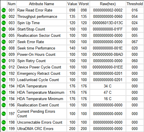
S.M.A.R.T. в HDDScan 3.3
В каждой строке отображается отдельный атрибут S.M.A.R.T. Атрибуты имеют более-менее стандартизованные названия и определённый номер, которые не зависят от модели и производителя диска.
Каждый атрибут S.M.A.R.T. имеет несколько полей. Каждое поле относится к определённому классу из следующих: ID, Value, Worst, Threshold и RAW. Рассмотрим каждый из классов.
- ID (может также именоваться Number) — идентификатор, номер атрибута в технологии S.M.A.R.T. Название одного и того же атрибута программами может выдаваться по-разному, а вот идентификатор всегда однозначно определяет атрибут. Особенно это полезно в случае программ, которые переводят общепринятое название атрибута с английского языка на русский. Иногда получается такая белиберда, что понять, что же это за параметр, можно только по его идентификатору.
- Value (Current) — текущее значение атрибута в попугаях (т. е. в величинах неизвестной размерности). В процессе работы винчестера оно может уменьшаться, увеличиваться и оставаться неизменным. По показателю Value нельзя судить о «здоровье» атрибута, не сравнивая его со значением Threshold этого же атрибута. Как правило, чем меньше Value, тем хуже состояние атрибута (изначально все классы значений, кроме RAW, на новом диске имеют максимальное из возможных значение, например 100).
- Worst — наихудшее значение, которого достигало значение Value за всю жизнь винчестера. Измеряется тоже в «попугаях». В процессе работы оно может уменьшаться либо оставаться неизменным. По нему тоже нельзя однозначно судить о здоровье атрибута, нужно сравнивать его с Threshold.
- Threshold — значение в «попугаях», которого должен достигнуть Value этого же атрибута, чтобы состояние атрибута было признано критическим. Проще говоря, Threshold — это порог: если Value больше Threshold — атрибут в порядке; если меньше либо равен — с атрибутом проблемы. Именно по такому критерию утилиты, читающие S.M.A.R.T., выдают отчёт о состоянии диска либо отдельного атрибута вроде «Good» или «Bad». При этом они не учитывают, что даже при Value, большем Threshold, диск на самом деле уже может быть умирающим с точки зрения пользователя, а то и вовсе ходячим мертвецом, поэтому при оценке здоровья диска смотреть стоит всё-таки на другой класс атрибута, а именно — RAW. Однако именно значение Value, опустившееся ниже Threshold, может стать легитимным поводом для замены диска по гарантии (для самих гарантийщиков, конечно же) — кто же яснее скажет о здоровье диска, как не он сам, демонстрируя текущее значение атрибута хуже критического порога? Т. е. при значении Value, большем Threshold, сам диск считает, что атрибут здоров, а при меньшем либо равном — что болен. Очевидно, что при Threshold=0 состояние атрибута не будет признано критическим никогда. Threshold — постоянный параметр, зашитый производителем в диске.
- RAW (Data) — самый интересный, важный и нужный для оценки показатель. В большинстве случаев он содержит в себе не «попугаи», а реальные значения, выражаемые в различных единицах измерения, напрямую говорящие о текущем состоянии диска. Основываясь именно на этом показателе, формируется значение Value (а вот по какому алгоритму оно формируется — это уже тайна производителя, покрытая мраком). Именно умение читать и анализировать поле RAW даёт возможность объективно оценить состояние винчестера.
Этим мы сейчас и займёмся — разберём все наиболее используемые атрибуты S.M.A.R.T., посмотрим, о чём они говорят и что нужно делать, если они не в порядке.
| Аттрибуты S.M.A.R.T. | |||||||||||||||||
| 01 | 02 | 03 | 04 | 05 | 07 | 08 | 09 | 10 | 11 | 12 | 183 | 184 | 187 | 188 | 189 | 190 | |
| 0x | 01 | 02 | 03 | 04 | 05 | 07 | 08 | 09 | 0A | 0B | 0C | B7 | B8 | BB | BC | BD | BE |
| 191 | 192 | 193 | 194 | 195 | 196 | 197 | 198 | 199 | 200 | 201 | 202 | 203 | 220 | 240 | 254 | ||
| 0x | BF | С0 | С1 | С2 | С3 | С4 | С5 | С6 | С7 | С8 | С9 | СА | CB | DC | F0 | FE |
Перед тем как описывать атрибуты и допустимые значения их поля RAW, уточню, что атрибуты могут иметь поле RAW разного типа: текущее и накапливающее. Текущее поле содержит значение атрибута в настоящий момент, для него свойственно периодическое изменение (для одних атрибутов — изредка, для других — много раз за секунду; другое дело, что в программах чтения S.M.A.R.T. такое быстрое изменение не отображается). Накапливающее поле — содержит статистику, обычно в нём содержится количество возникновений конкретного события со времени первого запуска диска.
Текущий тип характерен для атрибутов, для которых нет смысла суммировать их предыдущие показания. Например, показатель температуры диска является текущим: его цель — в демонстрации температуры в настоящий момент, а не суммы всех предыдущих температур. Накапливающий тип свойственен атрибутам, для которых весь их смысл заключается в предоставлении информации за весь период «жизни» винчестера. Например, атрибут, характеризующий время работы диска, является накапливающим, т. е. содержит количество единиц времени, отработанных накопителем за всю его историю.
Приступим к рассмотрению атрибутов и их RAW-полей.
Атрибут: 01 Raw Read Error Rate
| Тип | текущий, может быть накапливающим для WD и старых Hitachi |
| Описание | содержит частоту возникновения ошибок при чтении с пластин |
Для всех дисков Seagate, Samsung (начиная с семейства SpinPoint F1 (включительно)) и Fujitsu 2,5″ характерны огромные числа в этих полях.
Для остальных дисков Samsung и всех дисков WD в этом поле характерен 0.
Для дисков Hitachi в этом поле характерен 0 либо периодическое изменение поля в пределах от 0 до нескольких единиц.
Такие отличия обусловлены тем, что все жёсткие диски Seagate, некоторые Samsung и Fujitsu считают значения этих параметров не так, как WD, Hitachi и другие Samsung. При работе любого винчестера всегда возникают ошибки такого рода, и он преодолевает их самостоятельно, это нормально, просто на дисках, которые в этом поле содержат 0 или небольшое число, производитель не счёл нужным указывать истинное количество этих ошибок.
Таким образом, ненулевой параметр на дисках WD и Samsung до SpinPoint F1 (не включительно) и большое значение параметра на дисках Hitachi могут указывать на аппаратные проблемы с диском. Необходимо учитывать, что утилиты могут отображать несколько значений, содержащихся в поле RAW этого атрибута, как одно, и оно будет выглядеть весьма большим, хоть это и будет неверно (подробности см. ниже).
На дисках Seagate, Samsung (SpinPoint F1 и новее) и Fujitsu на этот атрибут можно не обращать внимания.
Атрибут: 02 Throughput Performance
| Тип | текущий |
| Описание | содержит значение средней производительности диска и измеряется в каких-то «попугаях». Обычно его ненулевое значение отмечается на винчестерах Hitachi. На них он может изменяться после изменения параметров ААМ, а может и сам по себе по неизвестному алгоритму |
Параметр не даёт никакой информации пользователю и не говорит ни о какой опасности при любом своём значении.
Атрибут: 03 Spin-Up Time
| Тип | текущий |
| Описание | содержит время, за которое шпиндель диска в последний раз разогнался из состояния покоя до номинальной скорости. Может содержать два значения — последнее и, например, минимальное время раскрутки. Может измеряться в миллисекундах, десятках миллисекунд и т. п. — это зависит от производителя и модели диска |
Время разгона может различаться у разных дисков (причём у дисков одного производителя тоже) в зависимости от тока раскрутки, массы блинов, номинальной скорости шпинделя и т. п.
Кстати, винчестеры Fujitsu всегда имеют единицу в этом поле в случае отсутствия проблем с раскруткой шпинделя.
Практически ничего не говорит о здоровье диска, поэтому при оценке состояния винчестера на параметр можно не обращать внимания.
Атрибут: 04 Number of Spin-Up Times (Start/Stop Count)
| Тип | накапливающий |
| Описание | содержит количество раз включения диска. Бывает ненулевым на только что купленном диске, находившемся в запаянной упаковке, что может говорить о тестировании диска на заводе. Или ещё о чём-то, мне не известном  |
При оценке здоровья не обращайте на атрибут внимания.
Атрибут: 05 Reallocated Sector Count
| Тип | накапливающий |
| Описание | содержит количество секторов, переназначенных винчестером в резервную область. Практически ключевой параметр в оценке состояния |
Поясним, что вообще такое «переназначенный сектор». Когда диск в процессе работы натыкается на нечитаемый/плохо читаемый/незаписываемый/плохо записываемый сектор, он может посчитать его невосполнимо повреждённым. Специально для таких случаев производитель предусматривает на каждом диске (на каких-то моделях — в центре (логическом конце) диска, на каких-то — в конце каждого трека и т. д.) резервную область. При наличии повреждённого сектора диск помечает его как нечитаемый и использует вместо него сектор в резервной области, сделав соответствующие пометки в специальном списке дефектов поверхности — G-list. Такая операция по назначению нового сектора на роль старого называется remap (ремап) либо переназначение, а используемый вместо повреждённого сектор — переназначенным. Новый сектор получает логический номер LBA старого, и теперь при обращении ПО к сектору с этим номером (программы же не знают ни о каких переназначениях!) запрос будет перенаправляться в резервную область.
Таким образом, хоть сектор и вышел из строя, объём диска не изменяется. Понятно, что не изменяется он до поры до времени, т. к. объём резервной области не бесконечен. Однако резервная область вполне может содержать несколько тысяч секторов, и допустить, чтобы она закончилась, будет весьма безответственно — диск нужно будет заменить задолго до этого.
Кстати, ремонтники говорят, что диски Samsung очень часто ни в какую не хотят выполнять переназначение секторов.
На счёт этого атрибута мнения разнятся. Лично я считаю, что если он достиг 10, диск нужно обязательно менять — ведь это означает прогрессирующий процесс деградации состояния поверхности либо блинов, либо головок, либо чего-то ещё аппаратного, и остановить этот процесс возможности уже нет. Кстати, по сведениям лиц, приближенных к Hitachi, сама Hitachi считает диск подлежащим замене, когда на нём находится уже 5 переназначенных секторов. Другой вопрос, официальная ли эта информация, и следуют ли этому мнению сервис-центры. Что-то мне подсказывает, что нет
Другое дело, что сотрудники сервис-центров могут отказываться признавать диск неисправным, если фирменная утилита производителя диска пишет что-то вроде «S.M.A.R.T. Status: Good» или значения Value либо Worst атрибута будут больше Threshold (собственно, по такому критерию может оценивать и сама утилита производителя). И формально они будут правы. Но кому нужен диск с постоянным ухудшением его аппаратных компонентов, даже если такое ухудшение соответствует природе винчестера, а технология производства жёстких дисков старается минимизировать его последствия, выделяя, например, резервную область?
Атрибут: 07 Seek Error Rate
| Тип | текущий |
| Описание | содержит частоту возникновения ошибок при позиционировании блока магнитных головок (БМГ) |
Описание формирования этого атрибута почти полностью совпадает с описанием для атрибута 01 Raw Read Error Rate, за исключением того, что для винчестеров Hitachi нормальным значением поля RAW является только 0.
Таким образом, на атрибут на дисках Seagate, Samsung SpinPoint F1 и новее и Fujitsu 2,5″ не обращайте внимания, на остальных моделях Samsung, а также на всех WD и Hitachi ненулевое значение свидетельствует о проблемах, например, с подшипником и т. п.
Атрибут: 08 Seek Time Performance
| Тип | текущий |
| Описание | содержит среднюю производительность операций позиционирования головок, измеряется в «попугаях». Как и параметр 02 Throughput Performance, ненулевое значение обычно отмечается на дисках Hitachi и может изменяться после изменения параметров ААМ, а может и само по себе по неизвестному алгоритму |
Не даёт никакой информации пользователю и не говорит ни о какой опасности при любом своём значении.
Атрибут: 09 Power On Hours Count (Power-on Time)
| Тип | накапливающий |
| Описание | содержит количество часов, в течение которых винчестер был включён |
Ничего не говорит о здоровье диска.
Атрибут: 10 (0А — в шестнадцатеричной системе счисления) Spin Retry Count
| Тип | накапливающий |
| Описание | содержит количество повторов запуска шпинделя, если первая попытка оказалась неудачной |
О здоровье диска чаще всего не говорит.
Основные причины увеличения параметра — плохой контакт диска с БП или невозможность БП выдать нужный ток в линию питания диска.
В идеале должен быть равен 0. При значении атрибута, равном 1-2, внимания можно не обращать. Если значение больше, в первую очередь следует обратить пристальное внимание на состояние блока питания, его качество, нагрузку на него, проверить контакт винчестера с кабелем питания, проверить сам кабель питания.
Наверняка диск может стартовать не сразу из-за проблем с ним самим, но такое бывает очень редко, и такую возможность нужно рассматривать в последнюю очередь.
Атрибут: 11 (0B) Calibration Retry Count (Recalibration Retries)
| Тип | накапливающий |
| Описание | содержит количество повторных попыток сброса накопителя (установки БМГ на нулевую дорожку) при неудачной первой попытке |
Ненулевое, а особенно растущее значение параметра может означать проблемы с диском.
Атрибут: 12 (0C) Power Cycle Count
| Тип | накапливающий |
| Описание | содержит количество полных циклов «включение-отключение» диска |
Не связан с состоянием диска.
Атрибут: 183 (B7) SATA Downshift Error Count
| Тип | накапливающий |
| Описание | содержит количество неудачных попыток понижения режима SATA. Суть в том, что винчестер, работающий в режимах SATA 3 Гбит/с или 6 Гбит/с (и что там дальше будет в будущем), по какой-то причине (например, из-за ошибок) может попытаться «договориться» с дисковым контроллером о менее скоростном режиме (например, SATA 1,5 Гбит/с или 3 Гбит/с соответственно). В случае «отказа» контроллера изменять режим диск увеличивает значение атрибута |
Не говорит о здоровье накопителя.
Атрибут: 184 (B8) End-to-End Error
| Тип | накапливающий |
| Описание | содержит количество ошибок, возникших при передаче данных через кэш винчестера |
Ненулевое значение указывает на проблемы с диском.
Атрибут: 187 (BB) Reported Uncorrected Sector Count (UNC Error)
| Тип | накапливающий |
| Описание | содержит количество секторов, которые были признаны кандидатами на переназначение (см. атрибут 197) за всю историю жизни диска. Причём если сектор становится кандидатом повторно, значение атрибута тоже увеличивается |
Ненулевое значение атрибута явно указывает на ненормальное состояние диска (в сочетании с ненулевым значением атрибута 197) или на то, что оно было таковым ранее (в сочетании с нулевым значением 197).
Атрибут: 188 (BC) Command Timeout
| Тип | накапливающий |
| Описание | содержит количество операций, выполнение которых было отменено из-за превышения максимально допустимого времени ожидания отклика |
Такие ошибки могут возникать из-за плохого качества кабелей, контактов, используемых переходников, удлинителей и т. д., а также из-за несовместимости диска с конкретным контроллером SATA/РАТА на материнской плате (либо дискретным). Из-за ошибок такого рода возможны BSOD в Windows.
Ненулевое значение атрибута говорит о потенциальной «болезни» диска.
Атрибут: 189 (BD) High Fly Writes
| Тип | накапливающий |
| Описание | содержит количество зафиксированных случаев записи при высоте полета головки выше рассчитанной — скорее всего, из-за внешних воздействий, например вибрации |
Для того чтобы сказать, почему происходят такие случаи, нужно уметь анализировать логи S.M.A.R.T., которые содержат специфичную для каждого производителя информацию, что на сегодняшний день не реализовано в общедоступном ПО — следовательно, на атрибут можно не обращать внимания.
Атрибут: 190 (BE) Airflow Temperature
| Тип | текущий |
| Описание | содержит температуру винчестера для дисков Hitachi, Samsung, WD и значение «100 − [RAW-значение атрибута 194]» для Seagate |
Не говорит о состоянии диска.
Атрибут: 191 (BF) G-Sensor Shock Count (Mechanical Shock)
| Тип | накапливающий |
| Описание | содержит количество критических ускорений, зафиксированных электроникой диска, которым подвергался накопитель и которые превышали допустимые. Обычно это происходит при ударах, падениях и т. п. |
Актуален для мобильных винчестеров. На дисках Samsung на него часто можно не обращать внимания, т. к. они могут иметь очень чувствительный датчик, который, образно говоря, реагирует чуть ли не на движение воздуха от крыльев пролетающей в одном помещении с диском мухи.
Вообще срабатывание датчика не является признаком удара. Может расти даже от позиционирования БМГ самим диском, особенно если его не закрепить. Основное назначение датчика — прекратить операцию записи при вибрациях, чтобы избежать ошибок.
Не говорит о здоровье диска.
Атрибут: 192 (С0) Power Off Retract Count (Emergency Retry Count)
| Тип | накапливающий |
| Описание | для разных винчестеров может содержать одну из следующих двух характеристик: либо суммарное количество парковок БМГ диска в аварийных ситуациях (по сигналу от вибродатчика, обрыву/понижению питания и т. п.), либо суммарное количество циклов включения/выключения питания диска (характерно для современных WD и Hitachi) |
Не позволяет судить о состоянии диска.
Атрибут: 193 (С1) Load/Unload Cycle Count
| Тип | накапливающий |
| Описание | содержит количество полных циклов парковки/распарковки БМГ. Анализ этого атрибута — один из способов определить, включена ли на диске функция автоматической парковки (столь любимая, например, компанией Western Digital): если его содержимое превосходит (обычно — многократно) содержимое атрибута 09 — счётчик отработанных часов, — то парковка включена |
Не говорит о здоровье диска.
Атрибут: 194 (С2) Temperature (HDA Temperature, HDD Temperature)
| Тип | текущий/накапливающий |
| Описание | содержит текущую температуру диска. Температура считывается с датчика, который на разных моделях может располагаться в разных местах. Поле вместе с текущей также может содержать максимальную и минимальную температуры, зафиксированные за всё время эксплуатации винчестера |
О состоянии диска атрибут не говорит, но позволяет контролировать один из важнейших параметров. Моё мнение: при работе старайтесь не допускать повышения температуры винчестера выше 50 градусов, хоть производителем обычно и декларируется максимальный предел температуры в 55-60 градусов.
Атрибут: 195 (С3) Hardware ECC Recovered
| Тип | накапливающий |
| Описание | содержит количество ошибок, которые были скорректированы аппаратными средствами ECC диска |
Особенности, присущие этому атрибуту на разных дисках, полностью соответствуют таковым атрибутов 01 и 07.
Атрибут: 196 (С4) Reallocated Event Count
| Тип | накапливающий |
| Описание | содержит количество операций переназначения секторов |
Косвенно говорит о здоровье диска. Чем больше значение — тем хуже. Однако нельзя однозначно судить о здоровье диска по этому параметру, не рассматривая другие атрибуты.
Этот атрибут непосредственно связан с атрибутом 05. При росте 196 чаще всего растёт и 05. Если при росте атрибута 196 атрибут 05 не растёт, значит, при попытке ремапа кандидат в бэд-блоки оказался софт-бэдом (подробности см. ниже), и диск исправил его, так что сектор был признан здоровым, и в переназначении не было необходимости.
Если атрибут 196 меньше атрибута 05, значит, во время некоторых операций переназначения выполнялся перенос нескольких повреждённых секторов за один приём.
Если атрибут 196 больше атрибута 05, значит, при некоторых операциях переназначения были обнаружены исправленные впоследствии софт-бэды.
Атрибут: 197 (С5) Current Pending Sector Count
| Тип | текущий |
| Описание | содержит количество секторов-кандидатов на переназначение в резервную область |
Натыкаясь в процессе работы на «нехороший» сектор (например, контрольная сумма сектора не соответствует данным в нём), диск помечает его как кандидат на переназначение, заносит его в специальный внутренний список и увеличивает параметр 197. Из этого следует, что на диске могут быть повреждённые секторы, о которых он ещё не знает — ведь на пластинах вполне могут быть области, которые винчестер какое-то время не использует.
При попытке записи в сектор диск сначала проверяет, не находится ли этот сектор в списке кандидатов. Если сектор там не найден, запись проходит обычным порядком. Если же найден, проводится тестирование этого сектора записью-чтением. Если все тестовые операции проходят нормально, то диск считает, что сектор исправен. (Т. е. был т. н. «софт-бэд» — ошибочный сектор возник не по вине диска, а по иным причинам: например, в момент записи информации отключилось электричество, и диск прервал запись, запарковав БМГ. В итоге данные в секторе окажутся недописанными, а контрольная сумма сектора, зависящая от данных в нём, вообще останется старой. Налицо будет расхождение между нею и данными в секторе.) В таком случае диск проводит изначально запрошенную запись и удаляет сектор из списка кандидатов. При этом атрибут 197 уменьшается, также возможно увеличение атрибута 196.
Если же тестирование заканчивается неудачей, диск выполняет операцию переназначения, уменьшая атрибут 197, увеличивая 196 и 05, а также делает пометки в G-list.
Итак, ненулевое значение параметра говорит о неполадках (правда, не может сказать о том, в само́м ли диске проблема).
При ненулевом значении нужно обязательно запустить в программах Victoria или MHDD последовательное чтение всей поверхности с опцией remap. Тогда при сканировании диск обязательно наткнётся на плохой сектор и попытается произвести запись в него (в случае Victoria 3.5 и опции Advanced remap — диск будет пытаться записать сектор до 10 раз). Таким образом программа спровоцирует «лечение» сектора, и в итоге сектор будет либо исправлен, либо переназначен.
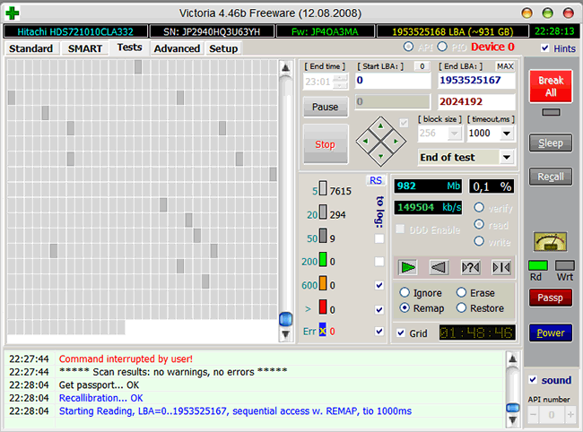
Идёт последовательное чтение с ремапом в Victoria 4.46b
В случае неудачи чтения как с remap, так и с Advanced remap, стоит попробовать запустить последовательную запись в тех же Victoria или MHDD. Учитывайте, что операция записи стирает данные, поэтому перед её применением обязательно делайте бэкап!
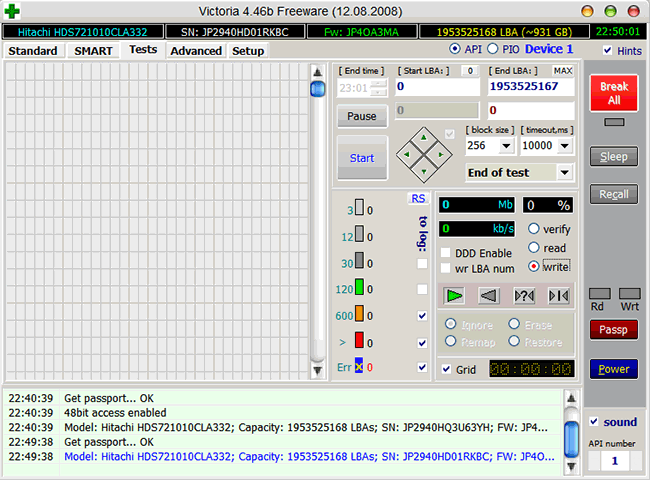
Запуск последовательной записи в Victoria 4.46b
Иногда от невыполнения ремапа могут помочь следующие манипуляции: снимите плату электроники диска и почистите контакты гермоблока винчестера, соединяющие его с платой — они могут быть окислены. Будь аккуратны при выполнении этой процедуры — из-за неё можно лишиться гарантии!
Невозможность ремапа может быть обусловлена ещё одной причиной — диск исчерпал резервную область, и ему просто некуда переназначать секторы.
Если же значение атрибута 197 никакими манипуляциями не снижается до 0, следует думать о замене диска.
Атрибут: 198 (С6) Offline Uncorrectable Sector Count (Uncorrectable Sector Count)
| Тип | текущий |
| Описание | означает то же самое, что и атрибут 197, но отличие в том, что данный атрибут содержит количество секторов-кандидатов, обнаруженных при одном из видов самотестирования диска — оффлайн-тестировании, которое диск запускает в простое в соответствии с параметрами, заданными прошивкой |
Параметр этот изменяется только под воздействием оффлайн-тестирования, никакие сканирования программами на него не влияют. При операциях во время самотестирования поведение атрибута такое же, как и атрибута 197.
Ненулевое значение говорит о неполадках на диске (точно так же, как и 197, не конкретизируя, кто виноват).
Атрибут: 199 (С7) UltraDMA CRC Error Count
| Тип | накапливающий |
| Описание | содержит количество ошибок, возникших при передаче по интерфейсному кабелю в режиме UltraDMA (или его эмуляции винчестерами SATA) от материнской платы или дискретного контроллера контроллеру диска |
В подавляющем большинстве случаев причинами ошибок становятся некачественный шлейф передачи данных, разгон шин PCI/PCI-E компьютера либо плохой контакт в SATA-разъёме на диске или на материнской плате/контроллере.
Ошибки при передаче по интерфейсу и, как следствие, растущее значение атрибута могут приводить к переключению операционной системой режима работы канала, на котором находится накопитель, в режим PIO, что влечёт резкое падение скорости чтения/записи при работе с ним и загрузку процессора до 100% (видно в Диспетчере задач Windows).
В случае винчестеров Hitachi серий Deskstar 7К3000 и 5К3000 растущий атрибут может говорить о несовместимости диска и SATA-контроллера. Чтобы исправить ситуацию, нужно принудительно переключить такой диск в режим SATA 3 Гбит/с.
Моё мнение: при наличии ошибок — переподключите кабель с обоих концов; если их количество растёт и оно больше 10 — выбрасывайте шлейф и ставьте вместо него новый или снимайте разгон.
Можно считать, что о здоровье диска атрибут не говорит.
Атрибут: 200 (С8) Write Error Rate (MultiZone Error Rate)
| Тип | текущий |
| Описание | содержит частоту возникновения ошибок при записи |
Ненулевое значение говорит о проблемах с диском — в частности, у дисков WD большие цифры могут означать «умирающие» головки.
Атрибут: 201 (С9) Soft Read Error Rate
| Тип | текущий |
| Описание | содержит частоту возникновения ошибок чтения, произошедших по вине программного обеспечения |
Влияние на здоровье неизвестно.
Атрибут: 202 (СА) Data Address Mark Error
| Тип | неизвестно |
| Описание | содержание атрибута — загадка, но проанализировав различные диски, могу констатировать, что ненулевое значение — это плохо |
Атрибут: 203 (CB) Run Out Cancel
| Тип | текущий |
| Описание | содержит количество ошибок ECC |
Влияние на здоровье неизвестно.
Атрибут: 220 (DC) Disk Shift
| Тип | текущий |
| Описание | содержит измеренный в неизвестных единицах сдвиг пластин диска относительно оси шпинделя |
Влияние на здоровье неизвестно.
Атрибут: 240 (F0) Head Flying Hours
| Тип | накапливающий |
| Описание | содержит время, затраченное на позиционирование БМГ. Счётчик может содержать несколько значений в одном поле |
Влияние на здоровье неизвестно.
Атрибут: 254 (FE) Free Fall Event Count
| Тип | накапливающий |
| Описание | содержит зафиксированное электроникой количество ускорений свободного падения диска, которым он подвергался, т. е., проще говоря, показывает, сколько раз диск падал |
Влияние на здоровье неизвестно.
Подытожим описание атрибутов. Ненулевые значения:
- атрибутов 01, 07, 195 — вызывают подозрения в «болезни» у некоторых моделей дисков;
- атрибутов 10, 11, 188, 196, 199, 202 — вызывают подозрения у всех дисков;
- и, наконец, атрибутов 05, 184, 187, 197, 198, 200 — прямо говорят о неполадках.
При анализе атрибутов учитывайте, что в некоторых параметрах S.M.A.R.T. могут храниться несколько значений этого параметра: например, для предпоследнего запуска диска и для последнего. Такие параметры длиной в несколько байт логически состоят из нескольких значений длиной в меньшее количество байт — например, параметр, хранящий два значения для двух последних запусков, под каждый из которых отводится 2 байта, будет иметь длину 4 байта. Программы, интерпретирующие S.M.A.R.T., часто не знают об этом, и показывают этот параметр как одно число, а не два, что иногда приводит к путанице и волнению владельца диска. Например, «Raw Read Error Rate», хранящий предпоследнее значение «1» и последнее значение «0», будет выглядеть как 65536.
Надо отметить, что не все программы умеют правильно отображать такие атрибуты. Многие как раз и переводят атрибут с несколькими значениями в десятичную систему счисления как одно огромное число. Правильно же отображать такое содержимое — либо с разбиением по значениям (тогда атрибут будет состоять из нескольких отдельных чисел), либо в шестнадцатеричной системе счисления (тогда атрибут будет выглядеть как одно число, но его составляющие будут легко различимы с первого взгляда), либо и то, и другое одновременно. Примерами правильных программ служат HDDScan, CrystalDiskInfo, Hard Disk Sentinel.
Продемонстрируем отличия на практике. Вот так выглядит мгновенное значение атрибута 01 на одном из моих Hitachi HDS721010CLA332 в неучитывающей особенности этого атрибута Victoria 4.46b:
![]()
Атрибут 01 в Victoria 4.46b
А так выглядит он же в «правильной» HDDScan 3.3:
![]()
Атрибут 01 в HDDScan 3.3
Плюсы HDDScan в данном контексте очевидны, не правда ли?
Если анализировать S.M.A.R.T. на разных дисках, то можно заметить, что одни и те же атрибуты могут вести себя по-разному. Например, некоторые параметры S.M.A.R.T. винчестеров Hitachi после определённого периода неактивности диска обнуляются; параметр 01 имеет особенности на дисках Hitachi, Seagate, Samsung и Fujitsu, 03 — на Fujitsu. Также известно, что после перепрошивки диска некоторые параметры могут установиться в 0 (например, 199). Однако подобное принудительное обнуление атрибута ни в коем случае не будет говорить о том, что проблемы с диском решены (если таковые были). Ведь растущий критичный атрибут — это следствие неполадок, а не причина.
При анализе множества массивов данных S.M.A.R.T. становится очевидным, что набор атрибутов у дисков разных производителей и даже у разных моделей одного производителя может отличаться. Связано это с так называемыми специфичными для конкретного вендора (vendor specific) атрибутами (т. е. атрибутами, используемыми для мониторинга своих дисков определённым производителем) и не должно являться поводом для волнения. Если ПО мониторинга умеет читать такие атрибуты (например, Victoria 4.46b), то на дисках, для которых они не предназначены, они могут иметь «страшные» (огромные) значения, и на них просто не нужно обращать внимания. Вот так, например, Victoria 4.46b отображает RAW-значения атрибутов, не предназначенных для мониторинга у Hitachi HDS721010CLA332:
«Страшные» значения в Victoria 4.46b
Нередко встречается проблема, когда программы не могут считать S.M.A.R.T. диска. В случае исправного винчестера это может быть вызвано несколькими факторами. Например, очень часто не отображается S.M.A.R.T. при подключении диска в режиме AHCI. В таких случаях стоит попробовать разные программы, в частности HDD Scan, которая обладает умением работать в таком режиме, хоть у неё и не всегда это получается, либо же стоит временно переключить диск в режим совместимости с IDE, если есть такая возможность. Далее, на многих материнских платах контроллеры, к которым подключаются винчестеры, бывают не встроенными в чипсет или южный мост, а реализованы отдельными микросхемами. В таком случае DOS-версия Victoria, например, не увидит подключённый к контроллеру жёсткий диск, и ей нужно будет принудительно указывать его, нажав клавишу [Р] и введя номер канала с диском. Часто не читаются S.M.A.R.T. у USB-дисков, что объясняется тем, что USB-контроллер просто не пропускает команды для чтения S.M.A.R.T. Практически никогда не читается S.M.A.R.T. у дисков, функционирующих в составе RAID-массива. Здесь тоже есть смысл попробовать разные программы, но в случае аппаратных RAID-контроллеров это бесполезно.
Если после покупки и установки нового винчестера какие-либо программы (HDD Life, Hard Drive Inspector и иже с ними) показывают, что: диску осталось жить 2 часа; его производительность — 27%; здоровье — 19,155% (выберите по вкусу) — то паниковать не стоит. Поймите следующее. Во-первых, нужно смотреть на показатели S.M.A.R.T., а не на непонятно откуда взявшиеся числа здоровья и производительности (впрочем, принцип их подсчёта понятен: берётся наихудший показатель). Во-вторых, любая программа при оценке параметров S.M.A.R.T. смотрит на отклонение значений разных атрибутов от предыдущих показаний. При первых запусках нового диска параметры непостоянны, необходимо некоторое время на их стабилизацию. Программа, оценивающая S.M.A.R.T., видит, что атрибуты изменяются, производит расчёты, у неё получается, что при их изменении такими темпами накопитель скоро выйдет из строя, и она начинает сигнализировать: «Спасайте данные!» Пройдёт некоторое время (до пары месяцев), атрибуты стабилизируются (если с диском действительно всё в порядке), утилита наберёт данных для статистики, и сроки кончины диска по мере стабилизации S.M.A.R.T. будут переноситься всё дальше и дальше в будущее. Оценка программами дисков Seagate и Samsung — вообще отдельный разговор. Из-за особенностей атрибутов 1, 7, 195 программы даже для абсолютно здорового диска обычно выдают заключение, что он завернулся в простыню и ползёт на кладбище.
Обратите внимание, что возможна следующая ситуация: все атрибуты S.M.A.R.T. — в норме, однако на самом деле диск — с проблемами, хоть этого пока ни по чему не заметно. Объясняется это тем, что технология S.M.A.R.T. работает только «по факту», т. е. атрибуты меняются только тогда, когда диск в процессе работы встречает проблемные места. А пока он на них не наткнулся, то и не знает о них и, следовательно, в S.M.A.R.T. ему фиксировать нечего.
Таким образом, S.M.A.R.T. — это полезная технология, но пользоваться ею нужно с умом. Кроме того, даже если S.M.A.R.T. вашего диска идеален, и вы постоянно устраиваете диску проверки — не полагайтесь на то, что ваш диск будет «жить» ещё долгие годы. Винчестерам свойственно ломаться так быстро, что S.M.A.R.T. просто не успевает отобразить его изменившееся состояние, а бывает и так, что с диском — явные нелады, но в S.M.A.R.T. — всё в порядке. Можно сказать, что хороший S.M.A.R.T. не гарантирует, что с накопителем всё хорошо, но плохой S.M.A.R.T. гарантированно свидетельствует о проблемах. При этом даже с плохим S.M.A.R.T. утилиты могут показывать, что состояние диска — «здоров», из-за того, что критичными атрибутами не достигнуты пороговые значения. Поэтому очень важно анализировать S.M.A.R.T. самому, не полагаясь на «словесную» оценку программ.
Хоть технология S.M.A.R.T. и работает, винчестеры и понятие «надёжность» настолько несовместимы, что принято считать их просто расходным материалом. Ну, как картриджи в принтере. Поэтому во избежание потери ценных данных делайте их периодическое резервное копирование на другой носитель (например, другой винчестер). Оптимально делать две резервные копии на двух разных носителях, не считая винчестера с оригинальными данными. Да, это ведёт к дополнительным затратам, но поверьте: затраты на восстановление информации со сломавшегося HDD обойдутся вам в разы — если не на порядок-другой — дороже. А ведь данные далеко не всегда могут восстановить даже профессионалы. Т. е. единственная возможность обеспечить надёжное хранение ваших данных — это делать их бэкап.
Напоследок упомяну некоторые программы, которые хорошо подходят для анализа S.M.A.R.T. и тестирования винчестеров: HDDScan (работает в Windows, бесплатная), CrystalDiskInfo (Windows, бесплатная), Hard Disk Sentinel (платная для Windows, бесплатная для DOS), HD Tune (Windows, платная, есть бесплатная старая версия).
И наконец, мощнейшие программы для тестирования: Victoria (Windows, DOS, бесплатная), MHDD (DOS, бесплатная).