1 Introduction
Minimum Bayes risk (MBR) training
[1, 2, 3]
has been shown to be an effective way to train neural net–based acoustic models
and is widely used for state-of-the-art speech recognition systems
[4, 5, 6].
MBR training minimizes an expected loss, where the loss measures the distance
between a reference and a hypothesis.
State-level MBR (sMBR) training
[7, 8]
is a popular form of MBR training which uses a loss defined at the frame level
based on clustered context-dependent phonemes or subphonemes.
It is computationally tractable, has an elegant lattice-based formulation using
the expectation semiring [9, 10],
and has been shown to perform favorably in terms of word error rate (WER)
compared to alternative losses that have been proposed
[8, 11].
Given the prevalence of word error rate as an evaluation metric, it is natural to
consider using it during MBR training.
We refer to this as
word-level edit-based MBR (word-level EMBR) training.
However expected word edit distance over a lattice is harder to compute than the
expected frame-level loss used by sMBR training.
As a result, many approximations to the true edit distance have been proposed for
lattice-based MBR training
[2, 12, 13, 7, 8, 14, 15].
Gibson provides a systematic review of the strengths and weaknesses of various
approximations [15, chapter 6].
Heigold et al. show that it is possible to exactly compute expected word edit
distance over a lattice by first expanding the lattice using an approach sometimes
termed error marking [16, 17].
While impressive, error marking is computationally and implementionally non-trivial,
and increases the size of the lattices.
The memory required for FST determinization during error marking increases rapidly
with utterance length, and van Dalen and Gales found a practical limit of around
10 words with the conventional determinization algorithm or around 20 words with
an improved, memory-efficient algorithm [17].
The time complexity also means error marking is unlikely to be compatible with
on-the-fly lattice generation.
In this paper we propose an alternative approach to lattice-based word-level EMBR
training.
The gradient of the expected loss optimized by MBR training may itself be written
as an expectation, allowing the gradient to be approximated by sampling.
The samples are paths through the lattice used during conventional sMBR training.
This approach is extremely flexible as it places almost no restriction on the form
of loss that may be used.
We use this approach to perform word-level EMBR training for two speech recognition
tasks and show that this improves WER compared to sMBR training.
To our knowledge this is also the first work to investigate word-level EMBR training
for state-of-the-art acoustic models based on neural nets.
Similar forms of sampled MBR training have been proposed previously.
Graves performed sampled EMBR training for the special case of a CTC model, noting
that the special structure of CTC allows trivial sampling and specialized approaches
to reduce the variance of the samples
[18]
.
Speech recognition may be viewed as a simple reinforcement learning problem where
an action consists of outputting a given word sequence.
In this view MBR training is learning a stochastic policy, and the sampling-based
approach described here is very similar to the
REINFORCE algorithm
[19, 20]
, though here we sample from a probability
distribution which is globally normalized instead of locally normalized, and there
are differences in the form of variance reduction used.
It should be noted that some previous investigations have reported better WER from
optimizing a state-level or phoneme-level criterion than a word-level criterion
[2] [15, chapter 7].
However some have reported the opposite [14].
We find the word-level criterion more effective in our experiments but do not
investigate this question systematically.
In the remainder of this paper we review the sequence-level probabilistic model
used by MBR training (§2 and §3), describe
MBR training (§4), discuss EMBR training
(§5), describe our sampling-based approach to MBR training
(§6), and describe our experimental results (§7).
2 FST-based probabilistic models
In this section we review how a weighted finite state transducer (FST)
[21] may be globally normalized to obtain a probabilistic
model.
The model used for MBR training is defined in this way.
A weighted FST defined over the real semiring (also called the probability
semiring) may naturally be turned into a probabilistic model over a sequence of
its output labels [22].
Each edge in the weighted FST has a real-valued weight and an
optional output label taken from a specified output alphabet, and an optional
input label taken from a specified input alphabet.
The absence of an input or output label is usually denoted with a special epsilon
label.
A path through the FST from the initial state to the final state111For simplicity we assume throughout that there is a single final state with
trivial final weight and no edges leaving it.
consists of a sequence of edges, and the weight of the path is defined
as the product of the weights of its edges.
The probability of a path is defined by globally normalizing this weight function:
This is a Markovian distribution.
The output label sequence associated with a path is the
sequence of non-epsilon output labels along the path.
The probability of a sequence of output labels is defined as the sum of the
probabilities of all paths consistent with :
3 Sequence-level model for recognition
In this section we briefly recap a conditional probabilistic model often used for
speech recognition.
This probabilistic model is an important component in sMBR training.
An acoustic model specifies a mapping
from an acoustic feature vector sequence to an
acoustic logit sequence given model parameters .
Each dimension
of the logit vector
is typically
associated with a cluster of context-dependent phonemes or sub-phonemes
[23].
In this paper the acoustic model is a stacked long short-term memory (LSTM)
network [24].
Given a logit sequence , we define a weighted FST as the composition
of a score FST and a decoder graph FST .
The decoder graph is itself a composition and incorporates weighted information
about context-dependence (C), pronunciation (L) and word sequence plausibility (G)
[25].
The score FST input and output alphabets and the decoder graph input alphabet are
.
The decoder graph output alphabet is the vocabulary.
We refer to as the unrolled decoder graph since composition with
effectively unrolls the decoder graph over time.
The score FST has a simple “sausage” structure with
states and an edge from state to state with input and output label
and log weight for each frame and cluster index .
The conditional probabilistic model over a word sequence
given an acoustic feature vector sequence
is obtained by applying the procedure described in §2 to the
unrolled decoder graph .
This gives
where and is the weight of a path.
It will be helpful to know the gradient of the log weight and log probability with
respect to the acoustic logits.
Due to the way the score FST is constructed, the sequence of non-epsilon input
labels encountered along a path through consists of a cluster index
for each frame .
The overall log weight has an additive contribution
from the acoustic model, and the gradient
consists of a matrix which has a one at for each frame
and zeros elsewhere.
The gradient of the log probability is given by
4 Minimum Bayes risk (MBR) training
Minimum Bayes risk (MBR) training
[1, 2, 3]
minimizes the expected loss222MBR training is named by analogy with MBR decoding [26],
but otherwise has little to do with Bayesian modeling or decision theory.
as a function of , where the loss specifies how bad
it is to output when the reference word sequence is .
Broadly speaking MBR concentrates probability mass:
a sufficiently flexible model trained to convergence with MBR will assign a
probability of to the word sequence(s) with smallest loss.
State-level minimum Bayes risk (sMBR) training
[7, 8]
defines the loss , now over instead of , to be
the number of frames at which the current cluster index differs from the reference
cluster index.
The sequence of time-aligned reference cluster indices is typically obtained
using forced alignment.
This loss has a number of disadvantages compared to minimizing the number of
word errors [15, chapter 6].
However it has the advantage that the expected loss and its gradient may be
computed tractably using an elegant formulation based on the
expectation semiring [9, 10].
The crucial property of the loss that makes it tractable is that the loss of
a path can be decomposed additively over the edges in the path.
Typically it is not feasible to perform sMBR training over the full unrolled
decoder graph , and a lattice containing a subset of paths is used
instead
[27, 4].
There has been some interest recently in performing exact “lattice-free”
sequence training using a simplified decoder graph [28].
5 Edit-based MBR (EMBR) training
Given the prevalence of word error rate (WER) as an evaluation metric,
a natural loss to use for MBR training is the edit distance between the
reference and hypothesized word sequences.
We refer to MBR training using a Levenshtein distance as the loss as
edit-based MBR (EMBR) training, and to using the number of word errors as
word-level EMBR training.
The number of word errors is the result of a dynamic programming computation and
does not decompose additively over the edges in a path, meaning the expectation
semiring approach cannot be applied without modification.
As discussed in §1, it is in fact possible to exactly compute the
expected number of word errors over a lattice by expanding the lattice using
error marking, but this approach produces larger lattices, in practice limits the
maximum utterance length, and is not compatible with on-the-fly lattice generation
[16, 17].
6 Sampled MBR training
In this section we look at a simple sampling-based approach to computing the MBR
loss value and its gradient.
This approach is essentially agnostic to the form of loss used, allowing us to
perform EMBR training simply and efficiently.
We consider the expected loss as a function of rather than
since
this provides the gradients required to implement sampled MBR in a modular
graph-of-operations framework such as TensorFlow
[29].
Samples from can be drawn efficiently using
backward filtering–forward sampling [30].
First the conventional backward algorithm is used to compute the sum of
the weights of all partial paths from each FST state to the final state.
The FST is then reweighted using as a potential function,
i.e. replacing the weight of each edge , which goes from some state
to some state , with [31].
This results in an equivalent FST which is locally normalized or stochastic,
i.e. the sum of edge weights leaving each state is one [31].
Samples from the reweighted FST can be drawn using simple ancestral sampling,
i.e. sample an edge leaving the initial state, then an edge leaving the end state
of the sampled edge, and repeat until we reach the final state.
In our implementation the values are computed once to draw multiple samples
and the reweighting is performed on-the-fly during sampling.
We can approximate the expected loss using a straightforward Monte Carlo
approximation:
where each is an independent sample from and
.
We write to denote averaging over samples.
The true gradient, writing for , is
This can be re-expressed using (5) as
Thus the MBR gradient is a scalar-vector covariance [10],
i.e. it is of the form
, and an unbiased
estimate is
We refer to using (12) during gradient-based training as
sampled MBR training.
It has the intuitive interpretation that samples with worse-than-average loss have
the log weight of the corresponding path reduced, and samples with better-than-average
loss have the log weight of the corresponding path increased.
The subtraction of in (12) makes the
estimated gradient invariant to an overall additive shift in loss, and may be seen
as performing variance reduction333Sampled MBR without variance reduction may be defined by approximating
as
.
The variance reduced version we have presented is equivalent to approximating
as
.
Both are unbiased estimates of the desired gradient since
.
,
often regarded as extremely important in sampling-based policy optimization for
reinforcement learning
[32, 33, 34].
Example code for sampled MBR training is shown in Figure 1.
Our implementation consisted of a TensorFlow op with input acoustic logits and
output expected loss.
def mbr(sample_path, collapse_path, get_gammas,
get_loss, num_samples, ref_labels):
paths = [sample_path()
for _ in range(num_samples)]
losses = [
get_loss(collapse_path(path), ref_labels)
for path in paths
]
mean_loss = np.mean(losses)
mean_gammas = sum([
get_gammas(path) * (loss — mean_loss)
for path, loss in zip(paths, losses)
]) / (num_samples — 1)
return mean_loss, mean_gammas
Here sample_path returns a sampled path from a lattice,
collapse_path ( in (2))
takes a path to a word sequence,
get_gammas takes a path to a matrix with a one
for each (frame, cluster index) which occurs in the path
(see §3), and
get_loss computes Levenshtein distance in the case of EMBR
training.
7 Experiments
We compared sMBR and sampled word-level EMBR training for two model architectures
on two speech recognition tasks.
7.1 CTC-style 2-channel Google Home model
We compared the performance of sMBR and EMBR training for a 2-channel query
recognition task (Google Home) using a CTC-style model where the set of clustered
context-dependent phonemes includes a blank symbol.
Our acoustic feature vector sequence was -dimensional with a
frame step, and consisted of a stack of three frames of log
mel filterbanks for each channel.
A stacked unidirectional LSTM acoustic model with layers of cells each
was used, followed by a linear layer with output dimension (the number of
clusters).
These “raw” logits were post-processed by applying log normalization with a
softmax-then-log then adding to the logit for CTC blank and scaling the
logits for the remaining clusters by to mimic what is often done during
decoding for CTC models; this post-processing does not seem to be critical for
good performance.
The initial CTC system was trained from a random initialization using
million
steps of asynchronous stochastic gradient descent, using context-dependent
phonemes as the reference label sequence.
The sMBR and EMBR systems were trained for a further
million steps, with the
best systems selected by WER on a small held-out dev set being obtained after a
total of roughly million and million steps respectively.
For both CTC and MBR training, each step computed the gradient on one whole
utterance.
Lattices for MBR training were generated on-the-fly.
Alignments for sMBR training were computed on-the-fly.
The decoder graph used during MBR training was constructed from a weak bigram
language model estimated on the training data, and a CTC-style context-dependent
C transducer with blank symbol was used [35].
EMBR training used samples per step.
The WER used during EMBR training was computed with language-specific capitalization
and punctuation normalization.
The learning rate for EMBR training was set times larger than for sMBR training
because the number of word errors is typically smaller than the number of frame
errors, and the typical gradient norm values during sMBR and EMBR training reflected
this.
We verified that using a times larger learning rate for sMBR was detrimental.
The training data was a voice search–specific subset of a corpus of around
million anonymized utterances with artificial room reverbation and noise added.
WER was evaluated on three corpora of anonymized -channel Google Home utterances.
WER on the dev set during training is presented in Figure 2.
Somewhat contrary to common wisdom that sMBR training converges quickly, we
observe WER continuing to improve for around million steps.
After billion total steps, sMBR training gets worse on the dev set and stays
roughly constant on the training set (not shown), meaning it is suffering from
overfitting.
EMBR training takes a long time to achieve its full gains; indeed it is not clear
it has converged even at billion total steps.
EMBR performance appears to be as good or better than sMBR after any number of
steps.
An EMBR step with samples in our set-up took around the same time as an
sMBR step.
EMBR has little overhead because sampling paths given the beta probabilities is
cheap and because overall computation time for both sMBR and EMBR is typically
dominated by the stacked LSTM computations and lattice generation.

and word-level EMBR (bottom).
The evaluation results are presented in Table 1.
We can see the sampled word-level EMBR training gave a 4–5 % relative gain
over sMBR training.
sMBR and word-level EMBR.
7.2 Non-CTC 1-channel voice search model
We also compared the performance of sMBR and EMBR training for a 1-channel voice
search task.
Our acoustic feature vector sequence was -dimensional with a
frame step, and consisted of a stack of four frames of log
mel filterbanks.
The stacked LSTM had layers of cells each.
An initial cross-entropy system was trained for million steps.
The sMBR and EMBR systems were trained for a futher million steps, and the
models with best WER on a held-out dev set were at around million and
million total steps respectively.
The systems were trained on a corpus of around million anonymized voice search
and dictation utterances with artificial reverb and noise added and evaluated on
four voice search test sets including one with noise added.
WER on the dev set during training is presented in Figure 3,
and results are presented in Table 2.
In these experiments we used the same learning rate for sMBR and EMBR training
since we were not yet fully aware of the mismatch in dynamic range; using a smaller
learning rate may improve sMBR performance.
We observed consistent gains from word-level EMBR training on this task.

(top) and word-level EMBR (bottom).
sMBR and word-level EMBR.
8 Conclusion
We have seen that sampled word-level EMBR training provides a simple and effective
way to optimize expected word error rate during training, and that this improves
empirical performance on two speech recognition tasks with disparate architectures.
9 Acknowledgements
Many thanks to Erik McDermott for his patient and helpful feedback on successive
drafts of this manuscript, and to Haşim Sak for many fruitful and enjoyable
discussions while implementing sMBR and EMBR training in TensorFlow.
References
-
[1]
J. Kaiser, B. Horvat, and Z. Kacic, “A novel loss function for the overall
risk criterion based discriminative training of HMM models,” inProc.
ICSLP, 2000. -
[2]
D. Povey and P. C. Woodland, “Minimum phone error and I-smoothing for
improved discriminative training,” in Proc. ICASSP, 2002. -
[3]
V. Doumpiotis and W. Byrne, “Pinched lattice minimum Bayes risk
discriminative training for large vocabulary continuous speech
recognition,” in Proc. Interspeech, 2004. -
[4]
B. Kingsbury, “Lattice-based optimization of sequence classification criteria
for neural-network acoustic modeling,” inProc. ICASSP, 2009.
-
[5]
H. Sak, A. Senior, K. Rao, and F. Beaufays, “Fast and accurate recurrent
neural network acoustic models for speech recognition,” inProc.
Interspeech, 2015. -
[6]
J. R. Bellegarda and C. Monz, “State of the art in statistical methods for
language and speech processing,” Computer Speech & Language,
vol. 35, pp. 163–184, 2016. -
[7]
M. Gibson and T. Hain, “Hypothesis spaces for minimum Bayes risk training in
large vocabulary speech recognition,” in Proc. Interspeech, 2006. -
[8]
D. Povey and B. Kingsbury, “Evaluation of proposed modifications to MPE for
large scale discriminative training,” in Proc. ICASSP, 2007. -
[9]
J. Eisner, “Expectation semirings: Flexible EM for learning finite-state
transducers,” in Proc. ESSLLI workshop on finite-state methods in
NLP, 2001. -
[10]
G. Heigold, T. Deselaers, R. Schlüter, and H. Ney, “Modified MMI/MPE: A
direct evaluation of the margin in speech recognition,” in Proc.
ICML, 2008. -
[11]
K. Veselỳ, A. Ghoshal, L. Burget, and D. Povey, “Sequence-discriminative
training of deep neural networks,” in Proc. Interspeech, 2013. -
[12]
J. Zheng and A. Stolcke, “Improved discriminative training using phone
lattices,” in Proc. Interspeech, 2005. -
[13]
W. Macherey, L. Haferkamp, R. Schlüter, and H. Ney, “Investigations on
error minimizing training criteria for discriminative training in automatic
speech recognition,” in Proc. Interspeech, 2005. -
[14]
Z.-J. Yan, B. Zhu, Y. Hu, and R.-H. Wang, “Minimum word classification error
training of HMMs for automatic speech recognition,” in Proc. ICASSP,
2008. -
[15]
M. Gibson, “Minimum Bayes risk acoustic model estimation and adaptation,”
Ph.D. dissertation, University of Sheffield, UK, 2008. -
[16]
G. Heigold, W. Macherey, R. Schluter, and H. Ney, “Minimum exact word error
training,” in Proc. ASRU, 2005. -
[17]
R. C. Van Dalen and M. J. Gales, “Annotating large lattices with the exact
word error,” in Proc. Interspeech, 2015. -
[18]
A. Graves and N. Jaitly, “Towards end-to-end speech recognition with
recurrent neural networks,” in Proc. ICML, 2014. -
[19]
R. J. Williams, “Simple statistical gradient-following algorithms for
connectionist reinforcement learning,” Machine learning, vol. 8, no.
3-4, pp. 229–256, 1992. -
[20]
M. Ranzato, S. Chopra, M. Auli, and W. Zaremba, “Sequence level training with
recurrent neural networks,” in Proc. ICLR, 2016. -
[21]
M. Mohri, F. Pereira, and M. Riley, “Weighted finite-state transducers in
speech recognition,” Computer Speech & Language, vol. 16, no. 1,
pp. 69–88, 2002. -
[22]
J. Eisner, “Parameter estimation for probabilistic finite-state
transducers,” in Proc. Association for Computational Linguistics,
2002. -
[23]
G. E. Dahl, D. Yu, L. Deng, and A. Acero, “Context-dependent pre-trained deep
neural networks for large-vocabulary speech recognition,” IEEE
Transactions on Audio, Speech, and Language Processing, vol. 20, no. 1, pp.
30–42, 2012. -
[24]
S. Hochreiter and J. Schmidhuber, “Long short-term memory,” Neural
computation, vol. 9, no. 8, pp. 1735–1780, 1997. -
[25]
M. Mohri, F. Pereira, and M. Riley, “Speech recognition with weighted
finite-state transducers,” in Springer Handbook of Speech
Processing, 2008, pp. 559–584. -
[26]
V. Goel and W. J. Byrne, “Minimum Bayes-risk automatic speech recognition,”
Computer Speech & Language, vol. 14, no. 2, pp. 115–135, 2000. -
[27]
V. Valtchev, J. Odell, P. C. Woodland, and S. J. Young, “Lattice-based
discriminative training for large vocabulary speech recognition,” in
Proc. ICASSP, 1996. -
[28]
D. Povey, V. Peddinti, D. Galvez, P. Ghahrmani, V. Manohar, X. Na, Y. Wang, and
S. Khudanpur, “Purely sequence-trained neural networks for ASR based on
lattice-free MMI,” 2016. -
[29]
M. Abadi, P. Barham, J. Chen, Z. Chen, A. Davis, J. Dean, M. Devin,
S. Ghemawat, G. Irving, M. Isard et al., “TensorFlow: A system for
large-scale machine learning,” in Proc. OSDI, 2016. -
[30]
H.-A. Loeliger and M. Molkaraie, “Estimating the partition function of 2-D
fields and the capacity of constrained noiseless 2-D channels using
tree-based Gibbs sampling,” in Proc. Information Theory Workshop,
2009, pp. 228–232. -
[31]
M. Mohri and M. Riley, “A weight pushing algorithm for large vocabulary
speech recognition,” in Proc. Interspeech, 2001. -
[32]
R. S. Sutton, D. A. McAllester, S. P. Singh, Y. Mansour et al.,
“Policy gradient methods for reinforcement learning with function
approximation,” in NIPS, vol. 99, 1999, pp. 1057–1063. -
[33]
F. Sehnke, C. Osendorfer, T. Rückstieß, A. Graves, J. Peters, and
J. Schmidhuber, “Parameter-exploring policy gradients,” Neural
Networks, vol. 23, no. 4, pp. 551–559, 2010. -
[34]
V. Mnih, N. Heess, A. Graves et al., “Recurrent models of visual
attention,” in Advances in neural information processing systems,
2014, pp. 2204–2212. -
[35]
H. Sak, A. Senior, K. Rao, O. Irsoy, A. Graves, F. Beaufays, and J. Schalkwyk,
“Learning acoustic frame labeling for speech recognition with recurrent
neural networks,” in Proc. ICASSP, 2015.
State-level minimum Bayes risk (sMBR) training has become the de facto
standard for sequence-level training of speech recognition acoustic models. It
has an elegant formulation using the expectation semiring, and gives large
improvements in word error rate (WER) over models trained solely using
cross-entropy (CE) or connectionist temporal classification (CTC). sMBR
training optimizes the expected number of frames at which the reference and
hypothesized acoustic states differ. It may be preferable to optimize the
expected WER, but WER does not interact well with the expectation semiring, and
previous approaches based on computing expected WER exactly involve expanding
the lattices used during training. In this paper we show how to perform
optimization of the expected WER by sampling paths from the lattices used
during conventional sMBR training. The gradient of the expected WER is itself
an expectation, and so may be approximated using Monte Carlo sampling. We show
experimentally that optimizing WER during acoustic model training gives 5%
relative improvement in WER over a well-tuned sMBR baseline on a 2-channel
query recognition task (Google Home).
PDF
Abstract
Code
No code implementations yet. Submit
your code now
Tasks
Datasets
Add Datasets
introduced or used in this paper
Results from the Paper
Submit
results from this paper
to get state-of-the-art GitHub badges and help the
community compare results to other papers.
Methods
No methods listed for this paper. Add
relevant methods here
If you’ve spent any time at all using an automatic speech recognition service, you may have seen the phrase “word error rate,” or WER, for short. But even if you’re brand new to transcriptions, WER is the most common metric you’ll see when comparing ASR services. Luckily, you don’t have to be a math whiz to figure it out – you just need to know this formula:
Word Error Rate = (Substitutions + Insertions + Deletions) / Number of Words Spoken
And that’s it! To go a bit more in depth, here’s how to effectively determine each of these factors:
- Substitutions are anytime a word gets replaced (for example, “twinkle” is transcribed as “crinkle”)
- Insertions are anytime a word gets added that wasn’t said (for example, “trailblazers” becomes “tray all blazers”)
- Deletions are anytime a word is omitted from the transcript (for example, “get it done” becomes “get done”)
Word Error Rate in Practice
Let’s take a look at an example audio.
The correct text is below:
We wanted people to know that we’ve got something brand new and essentially this product is, uh, what we call disruptive, changes the way that people interact with technology.
Now, here’s how that sentence was translated using Google’s speech to text API:
We wanted people to know that how to me where i know and essentially this product is what we call scripted changes the way people are rapid technology.
To correctly calculate WER, we take a look at the substitutions, insertions, and deletions between the two.

Add up the substitutions, insertions, and deletions, and you get a total of 11. Divide that by 29 (the total number of words spoken in the original file) to get a word error rate of about 38 percent. In some cases, the entire meaning of the sentence was changed.

Recently, we ran a test. We took 30 popular podcasts of varying topics and number of speakers, and transcribed them with Rev AI, Google, and Speechmatics. The overall WER for each service is below:
- Rev AI: 17.1%
- Google (video model): 18.3%
- Speechmatics: 21.3%
As these results suggest, you’ll get a different word error rate from whichever service you choose. And though WER is an important and standard metric, it’s not the only thing you should focus on.
The Power of Speaker Diarization
Are all of your transcriptions just one person narrating into a recorder? Great! You’ve somehow found the sweet spot of perfect audio.
What’s more likely, however, is that your files contain multiple speakers. Those speakers may sometimes cut each other off or talk over each other. They may even sound fairly similar.
One of the cool features of Rev AI is speaker diarization. This recognizes the different speakers in the room and attributes text to each. Whether it’s two people having an interview or a panel of four speakers, you can see who said what and when they said it. This is particularly useful if you’re planning to quote the speakers later. Imagine attributing a statement to the incorrect person – and even worse, getting the crux of their message wrong because of a high WER rate. You just may have two people upset with you: the actual speaker and the person you incorrectly cited.

Not all ASR services offer diarization, so keep that in mind if you’re often recording multiple people talking at once. You’ll want to be able to quickly discern between them.
Other Factors to Consider
WER can be an incredibly useful tool; however, it’s just one consideration when you’re choosing an ASR service.
A key thing to remember is that your WER will be inaccurate if you don’t normalize things like capitalization, punctuation, or numbers across your transcripts. Rev AI automatically transcribes spoken words into sentences and paragraphs. This is especially important if you are transcribing your audio files to increase accessibility. Transcripts formatted with these features will be significantly easier for your audience to read.
Word error rate can also be influenced by a number of additional factors, such as background noise, speaker volume, and regional dialects. Think about the times you’ve recorded someone or heard an interview during an event. Were you able to find a quiet, secure room away from all the hubbub? Did the speaker have a clear, booming voice? Chances are, there were some extenuating circumstances that didn’t allow for the perfect environment – and that’s just a part of life.
Certain ASR services are unable to distinguish sounds in these situations. Others, like Rev AI, can accurately transcribe the speakers no matter their volume or how far away they are from the recorder. Not everyone is going to have the lung capacity of Mick Jagger, and that’s fine. While we don’t require a minimum volume, other ASR services may. If you tend to interview quieter talkers or are in environments where you can’t make a lot of noise, be mindful of any requirements before making your selection.
Final Thoughts
Now that you’re comfortable calculating word error rate, you can feel more confident in your search for an ASR service. See how the power of a low WER can help your business reach new heights. Try Rev AI for free and get five hours of credit simply for signing up.
Try it free
The transcription industry has evolved a lot over the past 10 years. Academic and Healthcare firms remain the largest transcription customers. However, other industries such as financial, legal, manufacturing, and education also make up a significant percentage of the customer base.
Automatic Speech Recognition (ASR) software have made our daily routines more convenient. For instance, Alexa can now tell you how the weather will look like today.
Perhaps like most industries, transcription industry has been affected by ASR. This software are increasingly being used by various players that require transcripts. ASR is a cheap transcription solution. However, there is a big problem with the accuracy of ASR transcripts.
According to research comparing the accuracy rates of human transcriptionists and ASR software, human transcriptionists had an error rate of about 4% while commercially available ASR transcription software’s error rate was found to be 12%.
In a nutshell, the error rate of ASR is three times as bad as that of humans.
In 2017, Google announced that its voice recognition software had attained a Word Error Rate (WER) of about 4.7%. Is it really possible?
Let’s understand how ASR works and what are its implications in our transcription and translation industry.
What is Word Error Rate Mechanism (WER): By Definition
Word Error Rate (WER) is a common metric used to compare the accuracy of the transcripts produced by speech recognition APIs.
How to calculate WER (Word Error Rate Mechanism)
Here is a simple formula to understand how Word Error Rate (WER) is calculated:
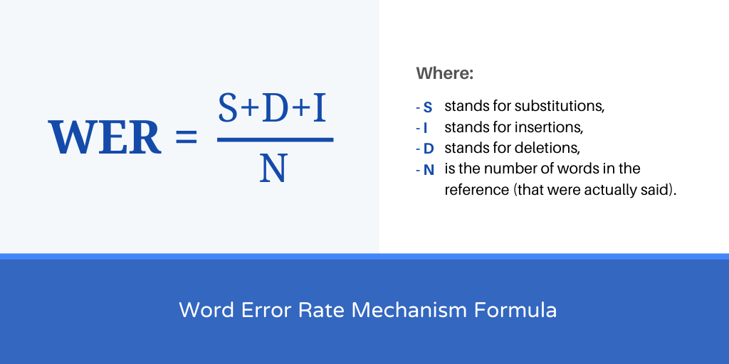
- S stands for substitutions,
- I stands for insertions,
- D stands for deletions,
- N is the number of words in the reference (that were actually said).
What Affects the Word Error Rate?
For speech recognition APIs like IBM Watson and Google Speech, a 25%-word error rate is about average for regular speech recognition. If the speech data is more technical, more “accented”, more industry-specific, and noisier, it becomes less likely that a general speech recognition API (or humans) will be more accurate.
Technical and Industry-specific Language
Human transcriptionists charge more for technical and industry-specific language, and there’s a reason for it. Reliably recognizing industry terms is complex and does take effort. Due to this, speech recognition systems trained on “average” data are found struggling with more specialized words.
Speaking with Different Accents and Dialects
What is construed as a strong accent in Dublin is normal in New York. Large companies like Google, Nuance and IBM have built speech recognition systems which are very familiar with “General American English” and British English. However, they may not be familiar with the different accents and dialects of English spoken in different cities around the world..
Disruptive Noise
Noisy audio and background noise is unwelcome but is common in many audio files. People rarely make business calls to us from a sound studio, or using VoIP and traditional phone systems compress audio that cut off many frequencies and add noise artifacts.
ASR Transcription Challenges and Word Error Rate Mechanism
Enterprise ASR software is built to understand a given accent and a limited number of words. For example, with some large companies their ASR software can recognize the National Switchboard Corpus, which is a popular database of words used in phone calls conversations that have already been transcribed.
Unfortunately, in the real world, audio files are different. For example, they may feature speakers with different accents or speaking different languages.
Also, most ASR software use WER to measure transcription errors. This measure has its shortfalls, such as:
- WER ignores the importance of words, giving the same score for each error in a document. In the real world, this isn’t accurate as some errors in a transcript matter compared to others.
- WER disregards punctuation and speaker labels.
- The test ignores the uhhs… and the mmhs…, duplicates and false starts that can interfere with the reading of your transcript.
Recent Research Findings on ASR
Researchers from leading companies like Google, Baidu, IBM, and Microsoft have been racing towards achieving the lowest-ever Word Error Rates from their speech recognition engines that has yielded remarkable results.
Gaining momentum from advances in neural networks and massive datasets compiled by them, WERs have improved to the extent of grabbing headlines about matching or even surpassing human efficiency.
Microsoft researchers, in contrast, report that their ASR engine has a WER of 5.1%, while for IBM Watson, it is 5.5%, and Google claims an error rate of just 4.9% (info source).
However, these tests were conducted by using a common set of audio recordings, i.e., a corpus called Switchboard, which consists of a large number of recordings of phone conversations covering a broad array of topics. Switchboard is a reasonable choice, as it has been used in the field for many years and is nearly ubiquitous in the current literature. Also, by testing against the audio corpus (database of speech audio files), researchers are able to make comparisons between themselves and competitors. Google is the lone exception, as it uses its own, internal test corpus (large structured set of texts).
This type of testing leads is limited as the claims of surpassing human transcriptionists are based on a very specific kind of audio. However, audio isn’t perfect or consistent and has many variables, and all of them can have a significant impact on transcription accuracy.
Is ASR Software’s WER Good Enough For Your Industry?
Stats reference:- An article written and shared by Andy Anderegg on Medium
ASR transcription accuracy rates don’t come close to the accuracy of human transcriptionists.
ASR transcription is also affected by cross talk, accents, background noise in the audio, and unknown words. In such instances, the accuracy will be poorer.
If you want to use ASR for transcription, be prepared to deal with:
- Inaccurate Transcripts
Accurate transcription is important, especially in the legal, business, and health industries. For instance, an inaccurate medical transcript can lead to a misdiagnosis and miscommunication.
ASR software produce more transcription errors than human transcriptionists. It is not uncommon to get a completely unintelligible transcript after using ASR. - Minimal Transcription Options
ASR software doesn’t have formatting or transcript options. The result will be transcripts that are not suited to your needs.
On the other hand, human transcriptionists can produce word to word or verbatim transcripts. - Different Speaking Styles
English is widely spoken in many parts of the world. However, there are considerable differences in the pronunciation and meaning of different words. People from different regions have their own way of speaking which is usually influenced by local dialects. Training voice recognition software to understand the various ways that English is spoken has proven to be quite difficult.
Transcription software also struggle when audio files have background noises. While AI has gotten incredibly good at reducing background noises in audio files, it is still far from perfect. If your file has background noises, you shouldn’t expect 100% accurate transcripts from using transcription software. - Ambiguous Vocabularies and Homophones
Transcription software also struggle to understand the context in speech. As a result, they cannot automatically detect missing parts of conversations in files. The inability to comprehend context can also lead to serious translation errors, which can have dire consequences in various industries. When words are spoken with a clear pause after every word, transcription software can easily and accurately transcribe the content. Therefore, the software would be best for dictations that revolve around short sentences.
However, in reality, humans speak in a more complex fashion. For example, some people talk softly while others talk faster when they are anxious. Transcription tools struggle to produce accurate transcripts in such contexts.
The Cost of Ignoring Quality Over Price
If you chose ASR transcription because it’s cheap, you will get low-quality transcripts full of errors. Such a transcript can cost you your business, money and even customers.
Here are two examples of businesses that had to pay dearly for machine-made transcription errors.
In 2006, Alitalia Airlines offered business class flights to its customers at a subsidized price of $39 compared to their usual $3900 price. Unknown to the customers, a copy-paste error had been made and the subsidized price was a mistake. More than 2000 customers had already booked the flight by the time the error was corrected. The customers wouldn’t accept the cancellation of their purchased tickets, and the airline had no choice but to reduce its prices leading to a loss of more than $7.2 million.
Another company, Fidelity Magellan Fund, had to cancel its dividend distribution when a transcription error saw it posting a capital gain of $1.3 billion rather than a loss of a similar amount. The transcription had omitted the negative sign causing the dividend estimate to be higher by $2.6million.
ASR transcription may be cheaper than human transcription. However, its errors can be costly. When you want accurate transcripts, human transcriptions are still the best option.
So, What Should You Do?
What is the way forward? Should you transition to automatic transcription or stay with the reliable manual transcription services provider?
Automatic transcription is fast and will save you time when you are on a deadline. However, in almost all cases, the transcripts will have to be brushed up for accuracy by professional transcriptionists.
Trained human transcriptionists can accurately identify complex terminology, accents, different dialects, and the presence of multiple speakers. The type of project should help you determine what form of transcription is best for you. If you are looking for highly accurate transcripts or work in a specialized industry like legal, academia, or medical, then working with a transcription company specialized in human transcription will be your best option.
Our Promise To You!
Unlike our peers, who have moved towards automated technology to gain a competitive cost advantage and maximize profits at the cost of accuracy, we stand our ground by only employing US-based human transcriptionist to whom we can trust for quality and confidentiality.
Our clients generally belong to different niche like legal, academic, businesses and more where quality matters above all. We have an unwavering commitment to client satisfaction, rather than mere concern for profit.