Ошибка округления это

Ошибки округления

Даже
если предположить, что исходная информация
не содержит никаких ошибок и все
вычислительные процессы конечны и не
приводят к ошибкам ограничения, то все
равно в этом случае присутствует третий
тип ошибок – ошибки округления.
Предположим, что вычисления производятся
на машине, в которой каждое число
представляется 5-ю значащими цифрами,
и что необходимо сложить два числа
9.2654 и 7.1625, причем эти два числа являются
точными. Сумма их равна 16.4279, она содержит
6 значащих цифр и не помещается в разрядной
сетке нашей гипотетической машины.
Поэтому 6-значный результат будет
округлен
до 16.428, и при этом возникает ошибка
округления.
Так как компьютеры всегда работают с
конечным числом значащих цифр, то
потребность в округлении возникает
довольно часто.

Вопросы
округления относятся только к
действительным числам. При выполнении
операций с целыми числами потребность
в округлении не возникает. Сумма, разность
и произведение целых чисел сами являются
целыми числами; если результат слишком
велик, то это свидетельствует об ошибке
в программе. Частное от деления двух
целых чисел не всегда является целым
числом, но при делении целых чисел
дробная часть отбрасывается.

Абсолютная и относительная погрешности

Допустим,
что точная ширина стола – А=384 мм, а мы,
измерив ее, получили а=381 мм. Модуль
разности между точным значением
измеряемой величины и ее приближенным
значением называется абсолютной
погрешностью
.
В данном примере абсолютная погрешность
3 мм. Но на практике мы никогда не знаем
точного значения измеряемой величины,
поэтому не можем точно знать абсолютную
погрешность.

Но
обычно мы знаем точность измерительных
приборов, опыт наблюдателя, производящего
измерения и т.д. Это дает возможность
составить представление об абсолютной
погрешности измерения. Если, например,
мы рулеткой измеряем длину комнаты, то
нам нетрудно учесть метры и сантиметры,
но вряд ли мы сможем учесть миллиметры.
Да в этом и нет надобности. Поэтому мы
сознательно допускаем ошибку в пределах
1 см. абсолютная погрешность длины
комнаты меньше 1 см. Измеряя длину
какого-либо отрезка миллиметровой
линейкой, мы имеем право утверждать,
что погрешность измерения не превышает
1 мм.

Абсолютная
погрешность _а
приближенного числа а дает возможность
установить границы, в которых лежит
точное число А:

Абсолютная
погрешность не является достаточным
показателем качества измерения и не
характеризует точность вычислений или
измерений. Если известно, что, измерив
некоторую длину, мы получили абсолютную
погрешность в 1 см, то никаких заключений
о том, хорошо или плохо мы измеряли,
сделать нельзя. Если мы измеряли длину
карандаша в 15 см и ошиблись на 1 см, наше
измерение никуда не годится. Если же мы
измеряли 20-метровый коридор и ошиблись
всего на 1 см, то наше измерение – образец
точности. Важна
не только сама абсолютная погрешность,
но и та доля, которую она составляет от
измеренной величины.
В первом примере абс. погрешность 1 см
составляет 1/15 долю измеряемой величины
или 7%, во втором – 1/2000 или 0.05%. Второе
измерение значительно лучше.

Относительной
погрешностью называют отношение
абсолютной погрешности к абсолютному
значению приближенной величины:

.

В
отличие от абсолютной погрешности,
которая обычно есть величина размерная,
относительная погрешность всегда есть
величина безразмерная. Обычно ее выражают
в %.

Пример

При измерении
длины в 5 см допущена абсолютная
погрешность в 0.1 см. Какова относительная
погрешность? (Ответ 2%)

При
подсчете числа жителей города, которое
оказалось равным 2
000
000,
допущена
погрешность 100 человек. Какова относительная
погрешность? (Ответ
0.005%)

Результат
всякого измерения выражается числом,
лишь приблизительно характеризующим
измеряемую величину. Поэтому при
вычислениях мы имеем дело с приближенными
числами. При записи приближенных чисел
принимается, что последняя цифра справа
характеризует величину абсолютной
погрешности.

Например,
если записано 12.45, то это не значит, что
величина, характеризуемая этим числом,
не содержит тысячных долей. Можно
утверждать, что тысячные доли при
измерении не учитывались, следовательно,
абсолютная погрешность меньше половины
единицы последнего разряда:
.
Аналогично, относительно приближенного
числа 1.283, можно сказать, что абсолютная
погрешность меньше 0.0005:.

Приближенные
числа принято записывать так, чтобы
абсолютная погрешность не превышала
единицы последнего десятичного разряда.
Или, иначе говоря, абсолютная
погрешность приближенного числа
характеризуется числом десятичных
знаков после запятой.

Как же
быть, если при тщательном измерении
какой-нибудь величины получится, что
она содержит целую единицу, 2 десятых,
5 сотых, не содержит тысячных, а
десятитысячные не поддаются учету? Если
записать 1.25, то в этой записи тысячные
не учтены, тогда как на самом деле мы
уверены, что их нет. В таком случае
принято ставить на их месте 0, – надо
писать 1.250. Таким образом, числа 1.25 и
1.250 обозначают не одно и то же. Первое –
содержит тысячные; мы только не знаем,
сколько именно. Второе – тысячных не
содержит, о десятитысячных ничего
сказать нельзя.

Сложнее
приходится при записи больших приближенных
чисел. Пусть число жителей деревни равно
2000 человек, а в городе приблизительно
457
000
жителей. Причем относительно города в
тысячах мы уверены, но допускаем
погрешность в сотнях и десятках. В первом
случае нули в конце числа указывают на
отсутствие сотен, десятков и единиц,
такие нули мы назовем значащими;
во втором случае нули указывают на наше
незнание числа сотен, десятков и единиц.
Такие нули мы назовем незначащими.
При записи приближенного числа,
содержащего нули надо дополнительно
оговаривать их значимость. Обычно нули
– незначащие. Иногда на незначимость
нулей можно указывать, записывая число
в экспоненциальном виде (457*10³).

Сравним
точность двух приближенных чисел 1362.3
и 2.37. В первом абсолютная погрешность
не превосходит 0.1, во втором – 0.01. Поэтому
второе число выглядит более точным, чем
первое.

Подсчитаем
относительную погрешность. Для первого
числа
;
для второго.
Второе число значительно (почти в 100
раз) менее точно, чем первое. Получается
это потому, что в первом числе дано 5
верных (значащих) цифр, тогда как во
втором – только 3.

Все
цифры приближенного числа, в которых
мы уверены, будем называть верными
(значащими) цифрами. Нули сразу справа
после запятой не бывают значащими, они
лишь указывают на порядок стоящих правее
значащих цифр. Нули в крайних правых
позициях числа могут быть как значащими,
так и не значащими. Например, каждое из
следующих чисел имеет 3 значащие цифры:
283*10⁵,
200*10²,
22.5, 0.0811, 2.10, 0.0000458.

Пример

Сколько
значащих (верных) цифр в следующих
числах:

0.75
(2), 12.050 (5), 1875*10⁵
(4), 0.06*10⁹
(1)

Оценить
относительную погрешность следующих
приближенных чисел:

0.989
(0.1%),

нули
значащие: 21000 (0.005%),

0.000
024
(4%),

0.05 (20%)

Нетрудно
заметить, что для примерной оценки
относительной погрешности числа
достаточно подсчитать количество
значащих цифр. Для числа, имеющего только
одну значащую цифру относительная
погрешность около 10%;

с
2-мя значащими цифрами – 1%;

с
3-мя значащими цифрами – 0.1%;

с
4-мя значащими цифрами – 0.01% и т.д.

При
вычислениях с приближенными числами
нас будет интересовать вопрос: как,
исходя из данных приближенных чисел,
получить ответ с нужной относительной
погрешностью.

Часто
при этом все исходные данные приходится
брать с одной и той же погрешностью,
именно с погрешностью наименее точного
из данных чисел. Поэтому часто приходится
более точное число заменять менее точным
– округлять.

округление
до десятых 27.136 
27.1,

округление
до целых 32.8 
33.

Правило
округления: Если крайняя левая из
отбрасываемых при округлении цифр
меньше 5, то последнюю сохраняемую цифру
не изменяют; если крайняя левая из
отбрасываемых цифр больше 5 или если
она равна 5, то последнюю сохраняемую
цифру увеличивают на 1.

Пример

округлить
до десятых 17.96 (18.0)

округлить
до сотых 14.127 (14.13)

округлить,
сохранив 3 верные цифры: 83.501 (83.5), 728.21
(728), 0.0168835 (0.01688).

Соседние файлы в предмете [НЕСОРТИРОВАННОЕ]

• #
• #
• #
• #
• #
• #
• #
• #
• #
• #
• #

Что такое ошибка округления?

Ошибка округления или ошибка округления – это математический просчет или ошибка квантования, вызванная изменением числа на целое или на число с меньшим количеством десятичных знаков. По сути, это разница между результатом математического алгоритма, использующего точную арифметику, и того же алгоритма, использующего несколько менее точную округленную версию того же числа или чисел. Значимость ошибки округления зависит от обстоятельств.

Хотя в большинстве случаев ошибка округления достаточно несущественна, чтобы ее игнорировать, она может иметь кумулятивный эффект в современной компьютеризированной финансовой среде, и в этом случае ее, возможно, придется исправить. Ошибка округления может быть особенно проблематичной, когда округленный ввод используется в серии вычислений, что приводит к увеличению ошибки, а иногда и к перевесу вычислений.

Термин «ошибка округления» также иногда используется для обозначения суммы, несущественной для очень большой компании.

Как работает ошибка округления

В финансовых отчетах многих компаний регулярно содержится предупреждение о том, что «цифры могут не совпадать из-за округления». В таких случаях очевидная ошибка вызвана только особенностями финансовой таблицы и не требует исправления.

Пример ошибки округления

Например, рассмотрим ситуацию, когда финансовое учреждение по ошибке округляет процентные ставки по ипотечным кредитам в конкретном месяце, в результате чего с его клиентов взимаются процентные ставки в размере 4% и 5% вместо 3,60% и 4,70% соответственно. В этом случае ошибка округления может затронуть десятки тысяч клиентов, а величина ошибки приведет к тому, что учреждение понесет сотни тысяч долларов расходов на исправление транзакций и исправление ошибки.

Бурный рост больших данных и связанных с ними передовых приложений для анализа данных только увеличил вероятность ошибок округления. Часто ошибка округления возникает случайно; это по своей природе непредсказуемо или иным образом трудно контролировать – отсюда и множество проблем, связанных с «чистыми данными» из больших данных. В других случаях ошибка округления возникает, когда исследователь по незнанию округляет переменную до нескольких десятичных знаков.

Для акробатических движений, округления см. Округлять.

А ошибка округления,^[1] также называемый ошибка округления,^[2] разница между результатом, полученным данным алгоритм с использованием точной арифметики и результата, полученного с помощью того же алгоритма с использованием округленной арифметики конечной точности.^[3] Ошибки округления возникают из-за неточности в представлении действительных чисел и выполняемых с ними арифметических операций. Это форма ошибка квантования.^[4] При использовании приближения уравнения или алгоритмов, особенно при использовании конечного числа цифр для представления действительных чисел (которые теоретически имеют бесконечно много цифр), одна из целей числовой анализ должен оценивать ошибки вычислений.^[5] Ошибки вычислений, также называемые числовые ошибки, включить оба ошибки усечения и ошибки округления.

Когда выполняется последовательность вычислений с вводом, содержащим ошибку округления, ошибки могут накапливаться, иногда доминируя при вычислении. В плохо воспитанный проблемы, может накапливаться значительная ошибка.^[6]

Короче говоря, в численных расчетах есть два основных аспекта ошибок округления:^[7]

1. Цифровые компьютеры имеют ограничения по величине и точности их способности представлять числа.
2. Некоторые числовые операции очень чувствительны к ошибкам округления. Это может быть связано как с математическими соображениями, так и с тем, как компьютеры выполняют арифметические операции.

Ошибка представления

Ошибка, возникающая при попытке представить число с помощью конечной строки цифр, является формой ошибки округления, называемой ошибка представления.^[8] Вот несколько примеров ошибок представления в десятичных представлениях:

Обозначение	Представление	Приближение	Ошибка
1/7	0.142 857	0.142 857	0.000 000 142 857
пер. 2	0.693 147 180 559 945 309 41…	0.693 147	0.000 000 180 559 945 309 41…
бревно10 2	0.301 029 995 663 981 195 21…	0.3010	0.000 029 995 663 981 195 21…
3√2	1.259 921 049 894 873 164 76…	1.25992	0.000 001 049 894 873 164 76…
√2	1.414 213 562 373 095 048 80…	1.41421	0.000 003 562 373 095 048 80…
е	2.718 281 828 459 045 235 36…	2.718 281 828 459 045	0.000 000 000 000 000 235 36…
π	3.141 592 653 589 793 238 46…	3.141 592 653 589 793	0.000 000 000 000 000 238 46…

Увеличение числа цифр, разрешенных в представлении, уменьшает величину возможных ошибок округления, но любое представление, ограниченное конечным числом цифр, все равно вызовет некоторую степень ошибки округления для бесчисленное множество действительные числа. Дополнительные цифры, используемые для промежуточных этапов расчета, известны как охранные цифры.^[9]

Многократное округление может привести к накоплению ошибок.^[10] Например, если 9,945309 округляется до двух десятичных знаков (9,95), а затем снова округляется до одного десятичного знака (10,0), общая ошибка составляет 0,054691. Округление 9,945309 до одного десятичного знака (9,9) за один шаг приводит к меньшей ошибке (0,045309). Обычно это происходит при выполнении арифметических операций (см. Потеря значимости ).

Система счисления с плавающей запятой

По сравнению с система счисления с фиксированной точкой, то система счисления с плавающей запятой более эффективен при представлении действительных чисел, поэтому широко используется в современных компьютерах. Пока реальные цифры бесконечны и непрерывны, система счисления с плавающей запятой конечно и дискретно. Таким образом, в системе счисления с плавающей точкой возникает ошибка представления, которая приводит к ошибке округления.

Обозначение системы счисления с плавающей запятой

Система счисления с плавающей запятой характеризуется целые числа:

: основание или основание

: точность

: диапазон экспоненты, где это нижняя граница и это верхняя граница

• Любой имеет следующий вид:

куда такое целое число, что за , и такое целое число, что .

Нормализованная система с плавающей запятой

, куда

считает выбор знака, положительный или отрицательный

считает выбор первой цифры

считает оставшуюся мантиссу

считает выбор показателей

считает тот случай, когда число .

Стандарт IEEE

в IEEE стандартная база двоичная, т.е. , и используется нормализация. Стандарт IEEE хранит знак, показатель степени и мантиссу в отдельных полях слова с плавающей запятой, каждое из которых имеет фиксированную ширину (количество бит). Два наиболее часто используемых уровня точности для чисел с плавающей запятой — это одинарная точность и двойная точность.

Точность	Знак (биты)	Экспонента (биты)	Мантисса (биты)
Одинокий	1	8	23
Двойной	1	11	52

Машина эпсилон

Машина эпсилон может использоваться для измерения уровня ошибки округления в системе счисления с плавающей запятой. Вот два разных определения.^[3]

Ошибка округления при разных правилах округления

Существует два общих правила округления: округление за отрезком и округление до ближайшего. Стандарт IEEE использует округление до ближайшего.

• Округление до ближайшего: устанавливается равным ближайшему числу с плавающей запятой к . Когда есть ничья, используется число с плавающей запятой, последняя сохраненная цифра которого четная.
  • Для стандарта IEEE, где базовый является , это означает, что когда есть ничья, она округляется так, чтобы последняя цифра была равна .
  • Это правило округления более точное, но более затратное с точки зрения вычислений.
  • Округление таким образом, чтобы последняя сохраненная цифра была даже при равенстве, гарантирует, что она не округляется систематически в большую или меньшую сторону. Это сделано для того, чтобы избежать возможности нежелательного медленного дрейфа в длинных вычислениях просто из-за смещения округления.

• В следующем примере показан уровень ошибки округления в соответствии с двумя правилами округления.^[3] Правило округления (округление до ближайшего) в целом приводит к меньшей ошибке округления.

Икс	По очереди	Ошибка округления	Округление до ближайшего	Ошибка округления
1.649	1.6	0.049	1.6	0.049
1.650	1.6	0.050	1.6	0.050
1.651	1.6	0.051	1.7	-0.049
1.699	1.6	0.099	1.7	-0.001
1.749	1.7	0.049	1.7	0.049
1.750	1.7	0.050	1.8	-0.050

Расчет ошибки округления в стандарте IEEE

Предположим, что используется округление до ближайшего и двойная точность IEEE.

• Пример: десятичное число может быть преобразован в

Поскольку бит справа от двоичной точки — это и за ним следуют другие ненулевые биты, правило округления до ближайшего требует округления, то есть добавления немного к кусочек. Таким образом, нормализованное представление с плавающей запятой в стандарте IEEE является

.

Это представление получается отбрасыванием бесконечного хвоста

из правого хвоста, а затем добавил на этапе округления.

потом .

Таким образом, ошибка округления равна .

Измерение ошибки округления с помощью машины эпсилон

Машина эпсилон может использоваться для измерения уровня ошибки округления при использовании двух вышеупомянутых правил округления. Ниже приведены формулы и соответствующие доказательства.^[3] Здесь используется первое определение машинного эпсилона.

Теорема

1. По очереди:
2. Округление до ближайшего:

Доказательство

Позволять куда , и разреши быть представлением с плавающей запятой . Поскольку используется последовательное нарезание,* Чтобы определить максимум этой величины, необходимо найти максимум числителя и минимум знаменателя. С (нормализованная система), минимальное значение знаменателя равно . Числитель ограничен сверху величиной . Таким образом, . Следовательно, для округления до ближайшего. Доказательство для округления до ближайшего аналогично.

• Обратите внимание, что первое определение машинного эпсилон не совсем эквивалентно второму определению при использовании правила округления до ближайшего, но оно эквивалентно для последовательного перехода.

Ошибка округления, вызванная арифметикой с плавающей запятой

Даже если некоторые числа могут быть представлены в точности числами с плавающей запятой и такие числа называются номера машин, выполнение арифметики с плавающей запятой может привести к ошибке округления в окончательном результате.

Добавление

Машинное сложение состоит из выстраивания десятичных знаков двух добавляемых чисел, их сложения и последующего сохранения результата как числа с плавающей запятой. Само сложение может быть выполнено с более высокой точностью, но результат должен быть округлен до указанной точности, что может привести к ошибке округления.^[3]

Например, добавив к в IEEE двойной точности следующим образом:

Из этого примера видно, что при сложении большого числа и малого числа может возникнуть ошибка округления, поскольку сдвиг десятичных знаков в мантиссах для согласования показателей степени может вызвать потерю некоторых цифр.

Умножение

В общем, продукт -цифровые мантиссы содержат до цифр, поэтому результат может не соответствовать мантиссе.^[3] Таким образом, в результат будет включена ошибка округления.

Разделение

В общем, частное -цифровые мантиссы могут содержать более -цифры.^[3] Таким образом, в результат будет включена ошибка округления.

Вычитающая отмена

Вычитание двух почти равных чисел называется вычитающее аннулирование.^[3]

Накопление ошибки округления

Ошибки могут увеличиваться или накапливаться, когда последовательность вычислений применяется к начальному входу с ошибкой округления из-за неточного представления.

Нестабильные алгоритмы

Алгоритм или численный процесс называется стабильный если небольшие изменения на входе вызывают только небольшие изменения на выходе, и это называется неустойчивый если производятся большие изменения на выходе.^[11]

Последовательность вычислений обычно происходит при запуске какого-либо алгоритма. Количество ошибок в результате зависит от стабильность алгоритма. Ошибка округления будет увеличиваться из-за нестабильных алгоритмов.

Например, за с данный. Легко показать, что . Предполагать это наше начальное значение и имеет небольшую ошибку представления , что означает, что начальный вход в этот алгоритм вместо . Затем алгоритм выполняет следующую последовательность вычислений.

Ошибка округления увеличивается в последующих вычислениях, поэтому этот алгоритм нестабилен.

Плохо обусловленные проблемы

Даже если используется стабильный алгоритм, решение проблемы все равно может быть неточным из-за накопления ошибки округления, когда сама проблема плохо воспитанный.

В номер условия Задачи — это отношение относительного изменения решения к относительному изменению на входе.^[3] Проблема в том хорошо кондиционированный если небольшие относительные изменения входных данных приводят к небольшим относительным изменениям в решении. В противном случае проблема в плохо воспитанный.^[3] Другими словами, проблема в том, плохо воспитанный если его число условия «намного больше», чем .

Число обусловленности вводится как мера ошибок округления, которые могут возникнуть при решении плохо обусловленных задач.^[7]

Например, многочлены высшего порядка имеют тенденцию быть очень плохо воспитанный, то есть они очень чувствительны к ошибке округления.^[7]

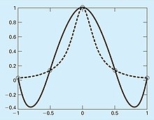
В 1901 г. Карл Рунге опубликовал исследование об опасностях полиномиальной интерполяции высокого порядка. Он посмотрел на следующую простую на вид функцию:

который сейчас называется Функция Рунге. Он взял равноудаленные точки данных из этой функции на интервале . Затем он использовал интерполяционные полиномы возрастающего порядка и обнаружил, что по мере того, как он брал больше точек, полиномы и исходная кривая значительно отличались, как показано на Рисунке «Сравнение1» и Рисунке «Сравнение 2». Дальше ситуация сильно ухудшилась с увеличением заказа. Как показано на Рисунке «Сравнение 2», посадка стала еще хуже, особенно в конце интервала.

Нажмите на рисунки, чтобы увидеть полное описание.

Пример из реального мира: отказ ракеты Patriot из-за увеличения ошибки округления

25 февраля 1991 года, во время войны в Персидском заливе, американская ракетная батарея «Пэтриот» в Дхаране, Саудовская Аравия, не смогла перехватить приближающуюся иракскую ракету «Скад». Скад врезался в казармы американской армии и убил 28 солдат. Отчет о Счетная палата правительства озаглавленный «Противоракетная оборона Patriot: проблема программного обеспечения, приведшая к отказу системы в Дахране, Саудовская Аравия», сообщает о причине сбоя: неточный расчет времени с момента загрузки из-за компьютерных арифметических ошибок. В частности, время в десятых долях секунды, измеренное внутренними часами системы, было умножено на 10, чтобы получить время в секундах. Этот расчет был выполнен с использованием 24-битного регистра с фиксированной точкой. В частности, значение 1/10, которое имеет неограниченное двоичное расширение, было прервано на 24 бита после точки счисления. Маленькая ошибка прерывания, умноженная на большое число, дающее время в десятых долях секунды, привела к значительной ошибке. Действительно, батарея Patriot проработала около 100 часов, и простой расчет показывает, что результирующая временная погрешность из-за увеличенной ошибки прерывания составила около 0,34 секунды. (Число 1/10 равно . Другими словами, двоичное разложение 1/10 равно . Теперь 24-битный регистр в Патриоте хранится вместо вводя ошибку двоичный, или около десятичный. Умножая на количество десятых долей секунды в часов дает ). Скад едет примерно 1676 метров в секунду, и поэтому за это время проходит более полукилометра. Этого было достаточно, чтобы приближающийся Скад находился за пределами «ворот дальности», которые отслеживал Патриот. По иронии судьбы, тот факт, что вычисление плохого времени было улучшено в некоторых частях кода, но не во всех, способствовал возникновению проблемы, поскольку это означало, что неточности не отменялись.^[12]

Смотрите также

• Точность (арифметика)
• Усечение
• Округление
• Потеря значимости
• Плавающая точка
• Алгоритм суммирования Кахана
• Машина эпсилон
• Полином Уилкинсона

Рекомендации

внешняя ссылка

• Ошибка округления в MathWorld.
• Гольдберг, Дэвид (Март 1991 г.). «Что должен знать каждый компьютерный ученый об арифметике с плавающей точкой» (PDF). Опросы ACM Computing. 23 (1): 5–48. Дои:10.1145/103162.103163. Получено 2016-01-20. ([1], [2] )
• 20 известных программных катастроф

Rounding means replacing a number with an approximate value that has a shorter, simpler, or more explicit representation. For example, replacing $23.4476 with $23.45, the fraction 312/937 with 1/3, or the expression √2 with 1.414.

Rounding is often done to obtain a value that is easier to report and communicate than the original. Rounding can also be important to avoid misleadingly precise reporting of a computed number, measurement, or estimate; for example, a quantity that was computed as 123,456 but is known to be accurate only to within a few hundred units is usually better stated as «about 123,500».

On the other hand, rounding of exact numbers will introduce some round-off error in the reported result. Rounding is almost unavoidable when reporting many computations – especially when dividing two numbers in integer or fixed-point arithmetic; when computing mathematical functions such as square roots, logarithms, and sines; or when using a floating-point representation with a fixed number of significant digits. In a sequence of calculations, these rounding errors generally accumulate, and in certain ill-conditioned cases they may make the result meaningless.

Accurate rounding of transcendental mathematical functions is difficult because the number of extra digits that need to be calculated to resolve whether to round up or down cannot be known in advance. This problem is known as «the table-maker’s dilemma».

Rounding has many similarities to the quantization that occurs when physical quantities must be encoded by numbers or digital signals.

A wavy equals sign (≈: approximately equal to) is sometimes used to indicate rounding of exact numbers, e.g., 9.98 ≈ 10. This sign was introduced by Alfred George Greenhill in 1892.^[1]

Ideal characteristics of rounding methods include:

1. Rounding should be done by a function. This way, when the same input is rounded in different instances, the output is unchanged.
2. Calculations done with rounding should be close to those done without rounding.
   • As a result of (1) and (2), the output from rounding should be close to its input, often as close as possible by some metric.
3. To be considered rounding, the range will be a subset of the domain, in general discrete. A classical range is the integers, Z.
4. Rounding should preserve symmetries that already exist between the domain and range. With finite precision (or a discrete domain), this translates to removing bias.
5. A rounding method should have utility in computer science or human arithmetic where finite precision is used, and speed is a consideration.

Because it is not usually possible for a method to satisfy all ideal characteristics, many different rounding methods exist.

As a general rule, rounding is idempotent;^[2] i.e., once a number has been rounded, rounding it again will not change its value. Rounding functions are also monotonic; i.e., rounding a larger number gives a larger or equal result than rounding a smaller number^{[clarification needed]}. In the general case of a discrete range, they are piecewise constant functions.

Types of rounding[edit]

Typical rounding problems include:

Rounding problem	Example input	Result	Rounding criterion
Approximating an irrational number by a fraction	π	22 / 7	1-digit-denominator
Approximating a rational number by another fraction with smaller numerator and denominator	399 / 941	3 / 7	1-digit-denominator
Approximating a fraction, which have periodic decimal expansion, by a finite decimal fraction	5 / 3	1.6667	4 decimal places
Approximating a fractional decimal number by one with fewer digits	2.1784	2.18	2 decimal places
Approximating a decimal integer by an integer with more trailing zeros	23,217	23,200	3 significant figures
Approximating a large decimal integer using scientific notation	300,999,999	3.01 × 108	3 significant figures
Approximating a value by a multiple of a specified amount	48.2	45	Multiple of 15
Rounding each one of a finite set of real numbers (mostly fractions) to an integer (sometimes the second-nearest integer) so that the sum of the rounded numbers equals the rounded sum of the numbers (needed e.g. [1] for the apportionment of seats, implemented e.g. by the largest remainder method, see Mathematics of apportionment, and [2] for distributing the total VAT of an invoice to its items)	{3/12, 4/12, 5/12}	{0, 0, 1}	Sum of rounded elements equals rounded sum of elements

Rounding to integer[edit]

The most basic form of rounding is to replace an arbitrary number by an integer. All the following rounding modes are concrete implementations of an abstract single-argument «round()» procedure. These are true functions (with the exception of those that use randomness).

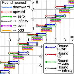
Directed rounding to an integer[edit]

These four methods are called directed rounding, as the displacements from the original number x to the rounded value y are all directed toward or away from the same limiting value (0, +∞, or −∞). Directed rounding is used in interval arithmetic and is often required in financial calculations.

If x is positive, round-down is the same as round-toward-zero, and round-up is the same as round-away-from-zero. If x is negative, round-down is the same as round-away-from-zero, and round-up is the same as round-toward-zero. In any case, if x is an integer, y is just x.

Where many calculations are done in sequence, the choice of rounding method can have a very significant effect on the result. A famous instance involved a new index set up by the Vancouver Stock Exchange in 1982. It was initially set at 1000.000 (three decimal places of accuracy), and after 22 months had fallen to about 520 — whereas stock prices had generally increased in the period. The problem was caused by the index being recalculated thousands of times daily, and always being rounded down to 3 decimal places, in such a way that the rounding errors accumulated. Recalculating with better rounding gave an index value of 1098.892 at the end of the same period.^[3]

For the examples below, sgn(x) refers to the sign function applied to the original number, x.

Rounding down[edit]

• round down (or take the floor, or round toward negative infinity): y is the largest integer that does not exceed x.

  

For example, 23.7 gets rounded to 23, and −23.2 gets rounded to −24.

Rounding up[edit]

• round up (or take the ceiling, or round toward positive infinity): y is the smallest integer that is not less than x.

  

For example, 23.2 gets rounded to 24, and −23.7 gets rounded to −23.

Rounding toward zero[edit]

• round toward zero (or truncate, or round away from infinity): y is the integer that is closest to x such that it is between 0 and x (included); i.e. y is the integer part of x, without its fraction digits.

  

For example, 23.7 gets rounded to 23, and −23.7 gets rounded to −23.

Rounding away from zero[edit]

• round away from zero (or round toward infinity): y is the integer that is closest to 0 (or equivalently, to x) such that x is between 0 and y (included).

  

For example, 23.2 gets rounded to 24, and −23.2 gets rounded to −24.

Rounding to the nearest integer[edit]

Rounding a number x to the nearest integer requires some tie-breaking rule for those cases when x is exactly half-way between two integers — that is, when the fraction part of x is exactly 0.5.

If it were not for the 0.5 fractional parts, the round-off errors introduced by the round to nearest method would be symmetric: for every fraction that gets rounded down (such as 0.268), there is a complementary fraction (namely, 0.732) that gets rounded up by the same amount.

When rounding a large set of fixed-point numbers with uniformly distributed fractional parts, the rounding errors by all values, with the omission of those having 0.5 fractional part, would statistically compensate each other. This means that the expected (average) value of the rounded numbers is equal to the expected value of the original numbers when numbers with fractional part 0.5 from the set are removed.

In practice, floating-point numbers are typically used, which have even more computational nuances because they are not equally spaced.

Rounding half up[edit]

The following tie-breaking rule, called round half up (or round half toward positive infinity), is widely used in many disciplines.^{[citation needed]} That is, half-way values of x are always rounded up.

• If the fractional part of x is exactly 0.5, then y = x + 0.5

  

For example, 23.5 gets rounded to 24, and −23.5 gets rounded to −23.

However, some programming languages (such as Java, Python) define their half up as round half away from zero here.^[4][5]

This method only requires checking one digit to determine rounding direction in two’s complement and similar representations.

Rounding half down[edit]

One may also use round half down (or round half toward negative infinity) as opposed to the more common round half up.

• If the fractional part of x is exactly 0.5, then y = x − 0.5

  

For example, 23.5 gets rounded to 23, and −23.5 gets rounded to −24.

However, some programming languages (such as Java, Python) define their half down as round half toward zero here.^[4][5]

Rounding half toward zero[edit]

One may also round half toward zero (or round half away from infinity) as opposed to the conventional round half away from zero.

• If the fractional part of x is exactly 0.5, then y = x − 0.5 if x is positive, and y = x + 0.5 if x is negative.

  

For example, 23.5 gets rounded to 23, and −23.5 gets rounded to −23.

This method treats positive and negative values symmetrically, and therefore is free of overall positive/negative bias if the original numbers are positive or negative with equal probability. It does, however, still have bias toward zero.

Rounding half away from zero[edit]

The other tie-breaking method commonly taught and used is the round half away from zero (or round half toward infinity), namely:

• If the fractional part of x is exactly 0.5, then y = x + 0.5 if x is positive, and y = x − 0.5 if x is negative.

  

For example, 23.5 gets rounded to 24, and −23.5 gets rounded to −24.

This can be more efficient on binary computers because only the first omitted bit needs to be considered to determine if it rounds up (on a 1) or down (on a 0). This is one method used when rounding to significant figures due to its simplicity.

This method, also known as commercial rounding,^{[citation needed]} treats positive and negative values symmetrically, and therefore is free of overall positive/negative bias if the original numbers are positive or negative with equal probability. It does, however, still have bias away from zero.

It is often used for currency conversions and price roundings (when the amount is first converted into the smallest significant subdivision of the currency, such as cents of a euro) as it is easy to explain by just considering the first fractional digit, independently of supplementary precision digits or sign of the amount (for strict equivalence between the paying and recipient of the amount).

Rounding half to even[edit]

A tie-breaking rule without positive/negative bias and without bias toward/away from zero is round half to even. By this convention, if the fractional part of x is 0.5, then y is the even integer nearest to x. Thus, for example, +23.5 becomes +24, as does +24.5; however, −23.5 becomes −24, as does −24.5. This function minimizes the expected error when summing over rounded figures, even when the inputs are mostly positive or mostly negative, provided they are neither mostly even nor mostly odd.

This variant of the round-to-nearest method is also called convergent rounding, statistician’s rounding, Dutch rounding, Gaussian rounding, odd–even rounding,^[6] or bankers’ rounding.

This is the default rounding mode used in IEEE 754 operations for results in binary floating-point formats, and the more sophisticated mode^{[clarification needed]} used when rounding to significant figures.

By eliminating bias, repeated addition or subtraction of independent numbers, as in a one-dimensional random walk, will give a rounded result with an error that tends to grow in proportion to the square root of the number of operations rather than linearly.

However, this rule distorts the distribution by increasing the probability of evens relative to odds. Typically this is less important^{[citation needed]} than the biases that are eliminated by this method.

Rounding half to odd[edit]

A similar tie-breaking rule to round half to even is round half to odd. In this approach, if the fractional part of x is 0.5, then y is the odd integer nearest to x. Thus, for example, +23.5 becomes +23, as does +22.5; while −23.5 becomes −23, as does −22.5.

This method is also free from positive/negative bias and bias toward/away from zero, provided the numbers to be rounded are neither mostly even nor mostly odd. It also shares the round half to even property of distorting the original distribution, as it increases the probability of odds relative to evens.

This variant is almost never used in computations, except in situations where one wants to avoid increasing the scale of floating-point numbers, which have a limited exponent range. With round half to even, a non-infinite number would round to infinity, and a small denormal value would round to a normal non-zero value. Effectively, this mode prefers preserving the existing scale of tie numbers, avoiding out-of-range results when possible for numeral systems of even radix (such as binary and decimal).^{[clarification needed (see talk)]}

Rounding to prepare for shorter precision[edit]

This rounding mode (RPSP in this chapter) is used to avoid getting wrong result with double (including multiple) rounding. With this rounding mode, one can avoid wrong result after double rounding, if all roundings except the final one are done using RPSP, and only final rounding uses the externally requested mode.

With decimal arithmetic, if there is a choice between numbers with the smallest significant digit 0 or 1, 4 or 5, 5 or 6, 9 or 0, then the digit different from 0 or 5 shall be selected; otherwise, choice is arbitrary. IBM defines ^[7] that, in the latter case, a digit with the smaller magnitude shall be selected. RPSP can be applied with the step between two consequent roundings as small as a single digit (for example, rounding to 1/10 can be applied after rounding to 1/100).
For example, when rounding to integer,

• 20.0 is rounded to 20;
• 20.01, 20.1, 20.9, 20.99, 21, 21.01, 21.9, 21.99 are rounded to 21;
• 22.0, 22.1, 22.9, 22.99 are rounded to 22;
• 24.0, 24.1, 24.9, 24.99 are rounded to 24;
• 25.0 is rounded to 25;
• 25.01, 25.1 are rounded to 26.

In the example from «Double rounding» section, rounding 9.46 to one decimal gives 9.4, which rounding to integer in turn gives 9.

With binary arithmetic, the rounding is made as «round to odd» (not to be mixed with «round half to odd».) For example, when rounding to 1/4:

• x == 2.0 => result is 2
• 2.0 < x < 2.5 => result is 2.25
• x == 2.5 => result is 2.5
• 2.5 < x < 3.0 => result is 2.75
• x == 3.0 => result is 3.0

For correct results, RPSP shall be applied with the step of at least 2 binary digits, otherwise, wrong result may appear. For example,

• 3.125 RPSP to 1/4 => result is 3.25
• 3.25 RPSP to 1/2 => result is 3.5
• 3.5 round-half-to-even to 1 => result is 4 (wrong)

If the step is 2 bits or more, RPSP gives 3.25 which, in turn, round-half-to-even to integer results in 3.

RPSP is implemented in hardware in IBM zSeries and pSeries.

Randomized rounding to an integer[edit]

Alternating tie-breaking[edit]

One method, more obscure than most, is to alternate direction when rounding a number with 0.5 fractional part. All others are rounded to the closest integer.

• Whenever the fractional part is 0.5, alternate rounding up or down: for the first occurrence of a 0.5 fractional part, round up, for the second occurrence, round down, and so on. Alternatively, the first 0.5 fractional part rounding can be determined by a random seed. «Up» and «down» can be any two rounding methods that oppose each other — toward and away from positive infinity or toward and away from zero.

If occurrences of 0.5 fractional parts occur significantly more than a restart of the occurrence «counting», then it is effectively bias free. With guaranteed zero bias, it is useful if the numbers are to be summed or averaged.

Random tie-breaking[edit]

• If the fractional part of x is 0.5, choose y randomly between x + 0.5 and x − 0.5, with equal probability. All others are rounded to the closest integer.

Like round-half-to-even and round-half-to-odd, this rule is essentially free of overall bias, but it is also fair among even and odd y values. An advantage over alternate tie-breaking is that the last direction of rounding on the 0.5 fractional part does not have to be «remembered».

Stochastic rounding[edit]

Rounding as follows to one of the closest integer toward negative infinity and the closest integer toward positive infinity, with a probability dependent on the proximity is called stochastic rounding and will give an unbiased result on average.^[8]

For example, 1.6 would be rounded to 1 with probability 0.4 and to 2 with probability 0.6.

Stochastic rounding can be accurate in a way that a rounding function can never be. For example, suppose one started with 0 and added 0.3 to that one hundred times while rounding the running total between every addition. The result would be 0 with regular rounding, but with stochastic rounding, the expected result would be 30, which is the same value obtained without rounding. This can be useful in machine learning where the training may use low precision arithmetic iteratively.^[8] Stochastic rounding is also a way to achieve 1-dimensional dithering.

Comparison of approaches for rounding to an integer[edit]

Value	Functional methods	Randomized methods
Directed rounding	Round to nearest	Round to prepare for shorter precision	Alternating tie-break	Random tie-break	Stochastic
Down (toward −∞)	Up (toward +∞)	Toward 0	Away From 0	Half Down (toward −∞)	Half Up (toward +∞)	Half Toward 0	Half Away From 0	Half to Even	Half to Odd	Average	SD	Average	SD	Average	SD
+1.8	+1	+2	+1	+2	+2	+2	+2	+2	+2	+2	+1	+2	0	+2	0	+1.8	0.04
+1.5	+1	+1	+1	+1.505	0	+1.5	0.05	+1.5	0.05
+1.2	+1	+1	+1	+1	0	+1	0	+1.2	0.04
+0.8	0	+1	0	+1	+0.8	0.04
+0.5	0	0	0	+0.505	0	+0.5	0.05	+0.5	0.05
+0.2	0	0	0	0	0	0	0	+0.2	0.04
−0.2	−1	0	−1	−1	−0.2	0.04
−0.5	−1	−1	−1	−0.495	0	−0.5	0.05	−0.5	0.05
−0.8	−1	−1	−1	−1	0	−1	0	−0.8	0.04
−1.2	−2	−1	−1	−2	−1.2	0.04
−1.5	−2	−2	−2	−1.495	0	−1.5	0.05	−1.5	0.05
−1.8	−2	−2	−2	−2	0	−2	0	−1.8	0.04

Rounding to other values[edit]

Rounding to a specified multiple[edit]

The most common type of rounding is to round to an integer; or, more generally, to an integer multiple of some increment — such as rounding to whole tenths of seconds, hundredths of a dollar, to whole multiples of 1/2 or 1/8 inch, to whole dozens or thousands, etc.

In general, rounding a number x to a multiple of some specified positive value m entails the following steps:

For example, rounding x = 2.1784 dollars to whole cents (i.e., to a multiple of 0.01) entails computing 2.1784 / 0.01 = 217.84, then rounding that to 218, and finally computing 218 × 0.01 = 2.18.

When rounding to a predetermined number of significant digits, the increment m depends on the magnitude of the number to be rounded (or of the rounded result).

The increment m is normally a finite fraction in whatever numeral system is used to represent the numbers. For display to humans, that usually means the decimal numeral system (that is, m is an integer times a power of 10, like 1/1000 or 25/100). For intermediate values stored in digital computers, it often means the binary numeral system (m is an integer times a power of 2).

The abstract single-argument «round()» function that returns an integer from an arbitrary real value has at least a dozen distinct concrete definitions presented in the rounding to integer section. The abstract two-argument «roundToMultiple()» function is formally defined here, but in many cases it is used with the implicit value m = 1 for the increment and then reduces to the equivalent abstract single-argument function, with also the same dozen distinct concrete definitions.

Logarithmic rounding[edit]

Rounding to a specified power[edit]

Rounding to a specified power is very different from rounding to a specified multiple; for example, it is common in computing to need to round a number to a whole power of 2. The steps, in general, to round a positive number x to a power of some positive number b other than 1, are:

Many of the caveats applicable to rounding to a multiple are applicable to rounding to a power.

Scaled rounding[edit]

This type of rounding, which is also named rounding to a logarithmic scale, is a variant of rounding to a specified power. Rounding on a logarithmic scale is accomplished by taking the log of the amount and doing normal rounding to the nearest value on the log scale.

For example, resistors are supplied with preferred numbers on a logarithmic scale. In particular, for resistors with a 10% accuracy, they are supplied with nominal values 100, 120, 150, 180, 220, etc. rounded to multiples of 10 (E12 series). If a calculation indicates a resistor of 165 ohms is required then log(150) = 2.176, log(165) = 2.217 and log(180) = 2.255. The logarithm of 165 is closer to the logarithm of 180 therefore a 180 ohm resistor would be the first choice if there are no other considerations.

Whether a value x ∈ (a, b) rounds to a or b depends upon whether the squared value x² is greater than or less than the product ab. The value 165 rounds to 180 in the resistors example because 165² = 27225 is greater than 150 × 180 = 27000.

Floating-point rounding[edit]

In floating-point arithmetic, rounding aims to turn a given value x into a value y with a specified number of significant digits. In other words, y should be a multiple of a number m that depends on the magnitude of x. The number m is a power of the base (usually 2 or 10) of the floating-point representation.

Apart from this detail, all the variants of rounding discussed above apply to the rounding of floating-point numbers as well. The algorithm for such rounding is presented in the Scaled rounding section above, but with a constant scaling factor s = 1, and an integer base b > 1.

Where the rounded result would overflow the result for a directed rounding is either the appropriate signed infinity when «rounding away from zero», or the highest representable positive finite number (or the lowest representable negative finite number if x is negative), when «rounding toward zero». The result of an overflow for the usual case of round to nearest is always the appropriate infinity.

Rounding to a simple fraction[edit]

In some contexts it is desirable to round a given number x to a «neat» fraction — that is, the nearest fraction y = m/n whose numerator m and denominator n do not exceed a given maximum. This problem is fairly distinct from that of rounding a value to a fixed number of decimal or binary digits, or to a multiple of a given unit m. This problem is related to Farey sequences, the Stern–Brocot tree, and continued fractions.

Rounding to an available value[edit]

Finished lumber, writing paper, capacitors, and many other products are usually sold in only a few standard sizes.

Many design procedures describe how to calculate an approximate value, and then «round» to some standard size using phrases such as «round down to nearest standard value», «round up to nearest standard value», or «round to nearest standard value».^[9][10]

When a set of preferred values is equally spaced on a logarithmic scale, choosing the closest preferred value to any given value can be seen as a form of scaled rounding. Such rounded values can be directly calculated.^[11]

Rounding in other contexts[edit]

Dithering and error diffusion[edit]

When digitizing continuous signals, such as sound waves, the overall effect of a number of measurements is more important than the accuracy of each individual measurement. In these circumstances, dithering, and a related technique, error diffusion, are normally used. A related technique called pulse-width modulation is used to achieve analog type output from an inertial device by rapidly pulsing the power with a variable duty cycle.

Error diffusion tries to ensure the error, on average, is minimized. When dealing with a gentle slope from one to zero, the output would be zero for the first few terms until the sum of the error and the current value becomes greater than 0.5, in which case a 1 is output and the difference subtracted from the error so far. Floyd–Steinberg dithering is a popular error diffusion procedure when digitizing images.

As a one-dimensional example, suppose the numbers 0.9677, 0.9204, 0.7451, and 0.3091 occur in order and each is to be rounded to a multiple of 0.01. In this case the cumulative sums, 0.9677, 1.8881 = 0.9677 + 0.9204, 2.6332 = 0.9677 + 0.9204 + 0.7451, and 2.9423 = 0.9677 + 0.9204 + 0.7451 + 0.3091, are each rounded to a multiple of 0.01: 0.97, 1.89, 2.63, and 2.94. The first of these and the differences of adjacent values give the desired rounded values: 0.97, 0.92 = 1.89 − 0.97, 0.74 = 2.63 − 1.89, and 0.31 = 2.94 − 2.63.

Monte Carlo arithmetic[edit]

Monte Carlo arithmetic is a technique in Monte Carlo methods where the rounding is randomly up or down. Stochastic rounding can be used for Monte Carlo arithmetic, but in general, just rounding up or down with equal probability is more often used. Repeated runs will give a random distribution of results which can indicate the stability of the computation.^[12]

Exact computation with rounded arithmetic[edit]

It is possible to use rounded arithmetic to evaluate the exact value of a function with integer domain and range. For example, if an integer n is known to be a perfect square, its square root can be computed by converting n to a floating-point value z, computing the approximate square root x of z with floating point, and then rounding x to the nearest integer y. If n is not too big, the floating-point round-off error in x will be less than 0.5, so the rounded value y will be the exact square root of n. This is essentially why slide rules could be used for exact arithmetic.

Double rounding[edit]

Rounding a number twice in succession to different levels of precision, with the latter precision being coarser, is not guaranteed to give the same result as rounding once to the final precision except in the case of directed rounding.^{[nb 1]} For instance rounding 9.46 to one decimal gives 9.5, and then 10 when rounding to integer using rounding half to even, but would give 9 when rounded to integer directly. Borman and Chatfield^[13] discuss the implications of double rounding when comparing data rounded to one decimal place to specification limits expressed using integers.

In Martinez v. Allstate and Sendejo v. Farmers, litigated between 1995 and 1997, the insurance companies argued that double rounding premiums was permissible and in fact required. The US courts ruled against the insurance companies and ordered them to adopt rules to ensure single rounding.^[14]

Some computer languages and the IEEE 754-2008 standard dictate that in straightforward calculations the result should not be rounded twice. This has been a particular problem with Java as it is designed to be run identically on different machines, special programming tricks have had to be used to achieve this with x87 floating point.^[15][16] The Java language was changed to allow different results where the difference does not matter and require a strictfp qualifier to be used when the results have to conform accurately; strict floating point has been restored in Java 17.^[17]

In some algorithms, an intermediate result is computed in a larger precision, then must be rounded to the final precision. Double rounding can be avoided by choosing an adequate rounding for the intermediate computation. This consists in avoiding to round to midpoints for the final rounding (except when the midpoint is exact). In binary arithmetic, the idea is to round the result toward zero, and set the least significant bit to 1 if the rounded result is inexact; this rounding is called sticky rounding.^[18] Equivalently, it consists in returning the intermediate result when it is exactly representable, and the nearest floating-point number with an odd significand otherwise; this is why it is also known as rounding to odd.^[19][20] A concrete implementation of this approach, for binary and decimal arithmetic, is implemented as Rounding to prepare for shorter precision.

Table-maker’s dilemma[edit]

William M. Kahan coined the term «The Table-Maker’s Dilemma» for the unknown cost of rounding transcendental functions:

Nobody knows how much it would cost to compute y^w correctly rounded for every two floating-point arguments at which it does not over/underflow. Instead, reputable math libraries compute elementary transcendental functions mostly within slightly more than half an ulp and almost always well within one ulp. Why can’t y^w be rounded within half an ulp like SQRT? Because nobody knows how much computation it would cost… No general way exists to predict how many extra digits will have to be carried to compute a transcendental expression and round it correctly to some preassigned number of digits. Even the fact (if true) that a finite number of extra digits will ultimately suffice may be a deep theorem.^[21]

The IEEE 754 floating-point standard guarantees that add, subtract, multiply, divide, fused multiply–add, square root, and floating-point remainder will give the correctly rounded result of the infinite-precision operation. No such guarantee was given in the 1985 standard for more complex functions and they are typically only accurate to within the last bit at best. However, the 2008 standard guarantees that conforming implementations will give correctly rounded results which respect the active rounding mode; implementation of the functions, however, is optional.

Using the Gelfond–Schneider theorem and Lindemann–Weierstrass theorem, many of the standard elementary functions can be proved to return transcendental results, except on some well-known arguments; therefore, from a theoretical point of view, it is always possible to correctly round such functions. However, for an implementation of such a function, determining a limit for a given precision on how accurate results need to be computed, before a correctly rounded result can be guaranteed, may demand a lot of computation time or may be out of reach.^[22] In practice, when this limit is not known (or only a very large bound is known), some decision has to be made in the implementation (see below); but according to a probabilistic model, correct rounding can be satisfied with a very high probability when using an intermediate accuracy of up to twice the number of digits of the target format plus some small constant (after taking special cases into account).

Some programming packages offer correct rounding. The GNU MPFR package gives correctly rounded arbitrary precision results. Some other libraries implement elementary functions with correct rounding in double precision:

• IBM’s ml4j, which stands for Mathematical Library for Java, written by Abraham Ziv and Moshe Olshansky in 1999, correctly rounded to nearest only.^[23][24] This library was claimed to be portable, but only binaries for PowerPC/AIX, SPARC/Solaris and x86/Windows NT were provided. According to its documentation, this library uses a first step with an accuracy a bit larger than double precision, a second step based on double-double arithmetic, and a third step with a 768-bit precision based on arrays of IEEE 754 double-precision floating-point numbers.
• IBM’s Accurate portable mathematical library (abbreviated as APMathLib or just MathLib),^[25][26] also called libultim,^[27] in rounding to nearest only. This library uses up to 768 bits of working precision. It was included in the GNU C Library in 2001,^[28] but the «slow paths» (providing correct rounding) were removed from 2018 to 2021.
• Sun Microsystems’s libmcr, in the 4 rounding modes.^[29] For the difficult cases, this library also uses multiple precision, and the number of words is increased by 2 each time the Table-maker’s dilemma occurs (with undefined behavior in the very unlikely event that some limit of the machine is reached).
• CRlibm, written in the old Arénaire team (LIP, ENS Lyon). It supports the 4 rounding modes and is proved, using the knowledge of the hardest-to-round cases.^[30][31]
• The CORE-MATH project provides some correctly rounded functions in the 4 rounding modes, using the knowledge of the hardest-to-round cases.^[32][33]

There exist computable numbers for which a rounded value can never be determined no matter how many digits are calculated. Specific instances cannot be given but this follows from the undecidability of the halting problem. For instance, if Goldbach’s conjecture is true but unprovable, then the result of rounding the following value up to the next integer cannot be determined: either 1+10⁻ⁿ where n is the first even number greater than 4 which is not the sum of two primes, or 1 if there is no such number. The rounded result is 2 if such a number n exists and 1 otherwise. The value before rounding can however be approximated to any given precision even if the conjecture is unprovable.

Interaction with string searches[edit]

Rounding can adversely affect a string search for a number. For example, π rounded to four digits is «3.1416» but a simple search for this string will not discover «3.14159» or any other value of π rounded to more than four digits. In contrast, truncation does not suffer from this problem; for example, a simple string search for «3.1415», which is π truncated to four digits, will discover values of π truncated to more than four digits.

History[edit]

The concept of rounding is very old, perhaps older than the concept of division itself. Some ancient clay tablets found in Mesopotamia contain tables with rounded values of reciprocals and square roots in base 60.^[34]
Rounded approximations to π, the length of the year, and the length of the month are also ancient—see base 60 examples.

The round-to-even method has served as the ASTM (E-29) standard since 1940. The origin of the terms unbiased rounding and statistician’s rounding are fairly self-explanatory. In the 1906 fourth edition of Probability and Theory of Errors^[35] Robert Simpson Woodward called this «the computer’s rule» indicating that it was then in common use by human computers who calculated mathematical tables. Churchill Eisenhart indicated the practice was already «well established» in data analysis by the 1940s.^[36]

The origin of the term bankers’ rounding remains more obscure. If this rounding method was ever a standard in banking, the evidence has proved extremely difficult to find. To the contrary, section 2 of the European Commission report The Introduction of the Euro and the Rounding of Currency Amounts^[37] suggests that there had previously been no standard approach to rounding in banking; and it specifies that «half-way» amounts should be rounded up.

Until the 1980s, the rounding method used in floating-point computer arithmetic was usually fixed by the hardware, poorly documented, inconsistent, and different for each brand and model of computer. This situation changed after the IEEE 754 floating-point standard was adopted by most computer manufacturers. The standard allows the user to choose among several rounding modes, and in each case specifies precisely how the results should be rounded. These features made numerical computations more predictable and machine-independent, and made possible the efficient and consistent implementation of interval arithmetic.

Currently, much research tends to round to multiples of 5 or 2. For example, Jörg Baten used age heaping in many studies, to evaluate the numeracy level of ancient populations. He came up with the ABCC Index, which enables the comparison of the numeracy among regions possible without any historical sources where the population literacy was measured.^[38]

Rounding functions in programming languages[edit]

Most programming languages provide functions or special syntax to round fractional numbers in various ways. The earliest numeric languages, such as FORTRAN and C, would provide only one method, usually truncation (toward zero). This default method could be implied in certain contexts, such as when assigning a fractional number to an integer variable, or using a fractional number as an index of an array. Other kinds of rounding had to be programmed explicitly; for example, rounding a positive number to the nearest integer could be implemented by adding 0.5 and truncating.

In the last decades, however, the syntax and the standard libraries of most languages have commonly provided at least the four basic rounding functions (up, down, to nearest, and toward zero). The tie-breaking method can vary depending on the language and version or might be selectable by the programmer. Several languages follow the lead of the IEEE 754 floating-point standard, and define these functions as taking a double-precision float argument and returning the result of the same type, which then may be converted to an integer if necessary. This approach may avoid spurious overflows because floating-point types have a larger range than integer types. Some languages, such as PHP, provide functions that round a value to a specified number of decimal digits (e.g., from 4321.5678 to 4321.57 or 4300). In addition, many languages provide a printf or similar string formatting function, which allows one to convert a fractional number to a string, rounded to a user-specified number of decimal places (the precision). On the other hand, truncation (round to zero) is still the default rounding method used by many languages, especially for the division of two integer values.

In contrast, CSS and SVG do not define any specific maximum precision for numbers and measurements, which they treat and expose in their DOM and in their IDL interface as strings as if they had infinite precision, and do not discriminate between integers and floating-point values; however, the implementations of these languages will typically convert these numbers into IEEE 754 double-precision floating-point values before exposing the computed digits with a limited precision (notably within standard JavaScript or ECMAScript^[39] interface bindings).

Other rounding standards[edit]

Some disciplines or institutions have issued standards or directives for rounding.

US weather observations[edit]

In a guideline issued in mid-1966,^[40] the U.S. Office of the Federal Coordinator for Meteorology determined that weather data should be rounded to the nearest round number, with the «round half up» tie-breaking rule. For example, 1.5 rounded to integer should become 2, and −1.5 should become −1. Prior to that date, the tie-breaking rule was «round half away from zero».

Negative zero in meteorology[edit]

Some meteorologists may write «−0» to indicate a temperature between 0.0 and −0.5 degrees (exclusive) that was rounded to an integer. This notation is used when the negative sign is considered important, no matter how small is the magnitude; for example, when rounding temperatures in the Celsius scale, where below zero indicates freezing.^{[citation needed]}

See also[edit]

• Cash rounding, dealing with the absence of extremely low-value coins
• Data binning, a similar operation
• Gal’s accurate tables
• Interval arithmetic
• ISO/IEC 80000
• Kahan summation algorithm
• Party-list proportional representation, an application of rounding to integers that has been thoroughly investigated
• Signed-digit representation
• Truncation

Notes[edit]

References[edit]

External links[edit]

• Weisstein, Eric W. «Rounding». MathWorld.
• An introduction to different rounding algorithms that is accessible to a general audience but especially useful to those studying computer science and electronics.
• How To Implement Custom Rounding Procedures by Microsoft (broken)

Rounding means replacing a number with an approximate value that has a shorter, simpler, or more explicit representation. For example, replacing $23.4476 with $23.45, the fraction 312/937 with 1/3, or the expression √2 with 1.414.

Rounding is often done to obtain a value that is easier to report and communicate than the original. Rounding can also be important to avoid misleadingly precise reporting of a computed number, measurement, or estimate; for example, a quantity that was computed as 123,456 but is known to be accurate only to within a few hundred units is usually better stated as «about 123,500».

On the other hand, rounding of exact numbers will introduce some round-off error in the reported result. Rounding is almost unavoidable when reporting many computations – especially when dividing two numbers in integer or fixed-point arithmetic; when computing mathematical functions such as square roots, logarithms, and sines; or when using a floating-point representation with a fixed number of significant digits. In a sequence of calculations, these rounding errors generally accumulate, and in certain ill-conditioned cases they may make the result meaningless.

Accurate rounding of transcendental mathematical functions is difficult because the number of extra digits that need to be calculated to resolve whether to round up or down cannot be known in advance. This problem is known as «the table-maker’s dilemma».

Rounding has many similarities to the quantization that occurs when physical quantities must be encoded by numbers or digital signals.

A wavy equals sign (≈: approximately equal to) is sometimes used to indicate rounding of exact numbers, e.g., 9.98 ≈ 10. This sign was introduced by Alfred George Greenhill in 1892.^[1]

Ideal characteristics of rounding methods include:

1. Rounding should be done by a function. This way, when the same input is rounded in different instances, the output is unchanged.
2. Calculations done with rounding should be close to those done without rounding.
   • As a result of (1) and (2), the output from rounding should be close to its input, often as close as possible by some metric.
3. To be considered rounding, the range will be a subset of the domain, in general discrete. A classical range is the integers, Z.
4. Rounding should preserve symmetries that already exist between the domain and range. With finite precision (or a discrete domain), this translates to removing bias.
5. A rounding method should have utility in computer science or human arithmetic where finite precision is used, and speed is a consideration.

Because it is not usually possible for a method to satisfy all ideal characteristics, many different rounding methods exist.

As a general rule, rounding is idempotent;^[2] i.e., once a number has been rounded, rounding it again will not change its value. Rounding functions are also monotonic; i.e., rounding a larger number gives a larger or equal result than rounding a smaller number^{[clarification needed]}. In the general case of a discrete range, they are piecewise constant functions.

Types of rounding[edit]

Typical rounding problems include:

Rounding problem	Example input	Result	Rounding criterion
Approximating an irrational number by a fraction	π	22 / 7	1-digit-denominator
Approximating a rational number by another fraction with smaller numerator and denominator	399 / 941	3 / 7	1-digit-denominator
Approximating a fraction, which have periodic decimal expansion, by a finite decimal fraction	5 / 3	1.6667	4 decimal places
Approximating a fractional decimal number by one with fewer digits	2.1784	2.18	2 decimal places
Approximating a decimal integer by an integer with more trailing zeros	23,217	23,200	3 significant figures
Approximating a large decimal integer using scientific notation	300,999,999	3.01 × 108	3 significant figures
Approximating a value by a multiple of a specified amount	48.2	45	Multiple of 15
Rounding each one of a finite set of real numbers (mostly fractions) to an integer (sometimes the second-nearest integer) so that the sum of the rounded numbers equals the rounded sum of the numbers (needed e.g. [1] for the apportionment of seats, implemented e.g. by the largest remainder method, see Mathematics of apportionment, and [2] for distributing the total VAT of an invoice to its items)	{3/12, 4/12, 5/12}	{0, 0, 1}	Sum of rounded elements equals rounded sum of elements

Rounding to integer[edit]

The most basic form of rounding is to replace an arbitrary number by an integer. All the following rounding modes are concrete implementations of an abstract single-argument «round()» procedure. These are true functions (with the exception of those that use randomness).

Directed rounding to an integer[edit]

These four methods are called directed rounding, as the displacements from the original number x to the rounded value y are all directed toward or away from the same limiting value (0, +∞, or −∞). Directed rounding is used in interval arithmetic and is often required in financial calculations.

If x is positive, round-down is the same as round-toward-zero, and round-up is the same as round-away-from-zero. If x is negative, round-down is the same as round-away-from-zero, and round-up is the same as round-toward-zero. In any case, if x is an integer, y is just x.

Where many calculations are done in sequence, the choice of rounding method can have a very significant effect on the result. A famous instance involved a new index set up by the Vancouver Stock Exchange in 1982. It was initially set at 1000.000 (three decimal places of accuracy), and after 22 months had fallen to about 520 — whereas stock prices had generally increased in the period. The problem was caused by the index being recalculated thousands of times daily, and always being rounded down to 3 decimal places, in such a way that the rounding errors accumulated. Recalculating with better rounding gave an index value of 1098.892 at the end of the same period.^[3]

For the examples below, sgn(x) refers to the sign function applied to the original number, x.

Rounding down[edit]

• round down (or take the floor, or round toward negative infinity): y is the largest integer that does not exceed x.

  

For example, 23.7 gets rounded to 23, and −23.2 gets rounded to −24.

Rounding up[edit]

• round up (or take the ceiling, or round toward positive infinity): y is the smallest integer that is not less than x.

  

For example, 23.2 gets rounded to 24, and −23.7 gets rounded to −23.

Rounding toward zero[edit]

• round toward zero (or truncate, or round away from infinity): y is the integer that is closest to x such that it is between 0 and x (included); i.e. y is the integer part of x, without its fraction digits.

  

For example, 23.7 gets rounded to 23, and −23.7 gets rounded to −23.

Rounding away from zero[edit]

• round away from zero (or round toward infinity): y is the integer that is closest to 0 (or equivalently, to x) such that x is between 0 and y (included).

  

For example, 23.2 gets rounded to 24, and −23.2 gets rounded to −24.

Rounding to the nearest integer[edit]

Rounding a number x to the nearest integer requires some tie-breaking rule for those cases when x is exactly half-way between two integers — that is, when the fraction part of x is exactly 0.5.

If it were not for the 0.5 fractional parts, the round-off errors introduced by the round to nearest method would be symmetric: for every fraction that gets rounded down (such as 0.268), there is a complementary fraction (namely, 0.732) that gets rounded up by the same amount.

When rounding a large set of fixed-point numbers with uniformly distributed fractional parts, the rounding errors by all values, with the omission of those having 0.5 fractional part, would statistically compensate each other. This means that the expected (average) value of the rounded numbers is equal to the expected value of the original numbers when numbers with fractional part 0.5 from the set are removed.

In practice, floating-point numbers are typically used, which have even more computational nuances because they are not equally spaced.

Rounding half up[edit]

The following tie-breaking rule, called round half up (or round half toward positive infinity), is widely used in many disciplines.^{[citation needed]} That is, half-way values of x are always rounded up.

• If the fractional part of x is exactly 0.5, then y = x + 0.5

  

For example, 23.5 gets rounded to 24, and −23.5 gets rounded to −23.

However, some programming languages (such as Java, Python) define their half up as round half away from zero here.^[4][5]

This method only requires checking one digit to determine rounding direction in two’s complement and similar representations.

Rounding half down[edit]

One may also use round half down (or round half toward negative infinity) as opposed to the more common round half up.

• If the fractional part of x is exactly 0.5, then y = x − 0.5

  

For example, 23.5 gets rounded to 23, and −23.5 gets rounded to −24.

However, some programming languages (such as Java, Python) define their half down as round half toward zero here.^[4][5]

Rounding half toward zero[edit]

One may also round half toward zero (or round half away from infinity) as opposed to the conventional round half away from zero.

• If the fractional part of x is exactly 0.5, then y = x − 0.5 if x is positive, and y = x + 0.5 if x is negative.

  

For example, 23.5 gets rounded to 23, and −23.5 gets rounded to −23.

This method treats positive and negative values symmetrically, and therefore is free of overall positive/negative bias if the original numbers are positive or negative with equal probability. It does, however, still have bias toward zero.

Rounding half away from zero[edit]

The other tie-breaking method commonly taught and used is the round half away from zero (or round half toward infinity), namely:

• If the fractional part of x is exactly 0.5, then y = x + 0.5 if x is positive, and y = x − 0.5 if x is negative.

  

For example, 23.5 gets rounded to 24, and −23.5 gets rounded to −24.

This can be more efficient on binary computers because only the first omitted bit needs to be considered to determine if it rounds up (on a 1) or down (on a 0). This is one method used when rounding to significant figures due to its simplicity.

This method, also known as commercial rounding,^{[citation needed]} treats positive and negative values symmetrically, and therefore is free of overall positive/negative bias if the original numbers are positive or negative with equal probability. It does, however, still have bias away from zero.

It is often used for currency conversions and price roundings (when the amount is first converted into the smallest significant subdivision of the currency, such as cents of a euro) as it is easy to explain by just considering the first fractional digit, independently of supplementary precision digits or sign of the amount (for strict equivalence between the paying and recipient of the amount).

Rounding half to even[edit]

A tie-breaking rule without positive/negative bias and without bias toward/away from zero is round half to even. By this convention, if the fractional part of x is 0.5, then y is the even integer nearest to x. Thus, for example, +23.5 becomes +24, as does +24.5; however, −23.5 becomes −24, as does −24.5. This function minimizes the expected error when summing over rounded figures, even when the inputs are mostly positive or mostly negative, provided they are neither mostly even nor mostly odd.

This variant of the round-to-nearest method is also called convergent rounding, statistician’s rounding, Dutch rounding, Gaussian rounding, odd–even rounding,^[6] or bankers’ rounding.

This is the default rounding mode used in IEEE 754 operations for results in binary floating-point formats, and the more sophisticated mode^{[clarification needed]} used when rounding to significant figures.

By eliminating bias, repeated addition or subtraction of independent numbers, as in a one-dimensional random walk, will give a rounded result with an error that tends to grow in proportion to the square root of the number of operations rather than linearly.

However, this rule distorts the distribution by increasing the probability of evens relative to odds. Typically this is less important^{[citation needed]} than the biases that are eliminated by this method.

Rounding half to odd[edit]

A similar tie-breaking rule to round half to even is round half to odd. In this approach, if the fractional part of x is 0.5, then y is the odd integer nearest to x. Thus, for example, +23.5 becomes +23, as does +22.5; while −23.5 becomes −23, as does −22.5.

This method is also free from positive/negative bias and bias toward/away from zero, provided the numbers to be rounded are neither mostly even nor mostly odd. It also shares the round half to even property of distorting the original distribution, as it increases the probability of odds relative to evens.

This variant is almost never used in computations, except in situations where one wants to avoid increasing the scale of floating-point numbers, which have a limited exponent range. With round half to even, a non-infinite number would round to infinity, and a small denormal value would round to a normal non-zero value. Effectively, this mode prefers preserving the existing scale of tie numbers, avoiding out-of-range results when possible for numeral systems of even radix (such as binary and decimal).^{[clarification needed (see talk)]}

Rounding to prepare for shorter precision[edit]

This rounding mode (RPSP in this chapter) is used to avoid getting wrong result with double (including multiple) rounding. With this rounding mode, one can avoid wrong result after double rounding, if all roundings except the final one are done using RPSP, and only final rounding uses the externally requested mode.

With decimal arithmetic, if there is a choice between numbers with the smallest significant digit 0 or 1, 4 or 5, 5 or 6, 9 or 0, then the digit different from 0 or 5 shall be selected; otherwise, choice is arbitrary. IBM defines ^[7] that, in the latter case, a digit with the smaller magnitude shall be selected. RPSP can be applied with the step between two consequent roundings as small as a single digit (for example, rounding to 1/10 can be applied after rounding to 1/100).
For example, when rounding to integer,

• 20.0 is rounded to 20;
• 20.01, 20.1, 20.9, 20.99, 21, 21.01, 21.9, 21.99 are rounded to 21;
• 22.0, 22.1, 22.9, 22.99 are rounded to 22;
• 24.0, 24.1, 24.9, 24.99 are rounded to 24;
• 25.0 is rounded to 25;
• 25.01, 25.1 are rounded to 26.

In the example from «Double rounding» section, rounding 9.46 to one decimal gives 9.4, which rounding to integer in turn gives 9.

With binary arithmetic, the rounding is made as «round to odd» (not to be mixed with «round half to odd».) For example, when rounding to 1/4:

• x == 2.0 => result is 2
• 2.0 < x < 2.5 => result is 2.25
• x == 2.5 => result is 2.5
• 2.5 < x < 3.0 => result is 2.75
• x == 3.0 => result is 3.0

For correct results, RPSP shall be applied with the step of at least 2 binary digits, otherwise, wrong result may appear. For example,

• 3.125 RPSP to 1/4 => result is 3.25
• 3.25 RPSP to 1/2 => result is 3.5
• 3.5 round-half-to-even to 1 => result is 4 (wrong)

If the step is 2 bits or more, RPSP gives 3.25 which, in turn, round-half-to-even to integer results in 3.

RPSP is implemented in hardware in IBM zSeries and pSeries.

Randomized rounding to an integer[edit]

Alternating tie-breaking[edit]

One method, more obscure than most, is to alternate direction when rounding a number with 0.5 fractional part. All others are rounded to the closest integer.

• Whenever the fractional part is 0.5, alternate rounding up or down: for the first occurrence of a 0.5 fractional part, round up, for the second occurrence, round down, and so on. Alternatively, the first 0.5 fractional part rounding can be determined by a random seed. «Up» and «down» can be any two rounding methods that oppose each other — toward and away from positive infinity or toward and away from zero.

If occurrences of 0.5 fractional parts occur significantly more than a restart of the occurrence «counting», then it is effectively bias free. With guaranteed zero bias, it is useful if the numbers are to be summed or averaged.

Random tie-breaking[edit]

• If the fractional part of x is 0.5, choose y randomly between x + 0.5 and x − 0.5, with equal probability. All others are rounded to the closest integer.

Like round-half-to-even and round-half-to-odd, this rule is essentially free of overall bias, but it is also fair among even and odd y values. An advantage over alternate tie-breaking is that the last direction of rounding on the 0.5 fractional part does not have to be «remembered».

Stochastic rounding[edit]

Rounding as follows to one of the closest integer toward negative infinity and the closest integer toward positive infinity, with a probability dependent on the proximity is called stochastic rounding and will give an unbiased result on average.^[8]

For example, 1.6 would be rounded to 1 with probability 0.4 and to 2 with probability 0.6.

Stochastic rounding can be accurate in a way that a rounding function can never be. For example, suppose one started with 0 and added 0.3 to that one hundred times while rounding the running total between every addition. The result would be 0 with regular rounding, but with stochastic rounding, the expected result would be 30, which is the same value obtained without rounding. This can be useful in machine learning where the training may use low precision arithmetic iteratively.^[8] Stochastic rounding is also a way to achieve 1-dimensional dithering.

Comparison of approaches for rounding to an integer[edit]

Value	Functional methods	Randomized methods
Directed rounding	Round to nearest	Round to prepare for shorter precision	Alternating tie-break	Random tie-break	Stochastic
Down (toward −∞)	Up (toward +∞)	Toward 0	Away From 0	Half Down (toward −∞)	Half Up (toward +∞)	Half Toward 0	Half Away From 0	Half to Even	Half to Odd	Average	SD	Average	SD	Average	SD
+1.8	+1	+2	+1	+2	+2	+2	+2	+2	+2	+2	+1	+2	0	+2	0	+1.8	0.04
+1.5	+1	+1	+1	+1.505	0	+1.5	0.05	+1.5	0.05
+1.2	+1	+1	+1	+1	0	+1	0	+1.2	0.04
+0.8	0	+1	0	+1	+0.8	0.04
+0.5	0	0	0	+0.505	0	+0.5	0.05	+0.5	0.05
+0.2	0	0	0	0	0	0	0	+0.2	0.04
−0.2	−1	0	−1	−1	−0.2	0.04
−0.5	−1	−1	−1	−0.495	0	−0.5	0.05	−0.5	0.05
−0.8	−1	−1	−1	−1	0	−1	0	−0.8	0.04
−1.2	−2	−1	−1	−2	−1.2	0.04
−1.5	−2	−2	−2	−1.495	0	−1.5	0.05	−1.5	0.05
−1.8	−2	−2	−2	−2	0	−2	0	−1.8	0.04

Rounding to other values[edit]

Rounding to a specified multiple[edit]

The most common type of rounding is to round to an integer; or, more generally, to an integer multiple of some increment — such as rounding to whole tenths of seconds, hundredths of a dollar, to whole multiples of 1/2 or 1/8 inch, to whole dozens or thousands, etc.

In general, rounding a number x to a multiple of some specified positive value m entails the following steps:

For example, rounding x = 2.1784 dollars to whole cents (i.e., to a multiple of 0.01) entails computing 2.1784 / 0.01 = 217.84, then rounding that to 218, and finally computing 218 × 0.01 = 2.18.

When rounding to a predetermined number of significant digits, the increment m depends on the magnitude of the number to be rounded (or of the rounded result).

The increment m is normally a finite fraction in whatever numeral system is used to represent the numbers. For display to humans, that usually means the decimal numeral system (that is, m is an integer times a power of 10, like 1/1000 or 25/100). For intermediate values stored in digital computers, it often means the binary numeral system (m is an integer times a power of 2).

The abstract single-argument «round()» function that returns an integer from an arbitrary real value has at least a dozen distinct concrete definitions presented in the rounding to integer section. The abstract two-argument «roundToMultiple()» function is formally defined here, but in many cases it is used with the implicit value m = 1 for the increment and then reduces to the equivalent abstract single-argument function, with also the same dozen distinct concrete definitions.

Logarithmic rounding[edit]

Rounding to a specified power[edit]

Rounding to a specified power is very different from rounding to a specified multiple; for example, it is common in computing to need to round a number to a whole power of 2. The steps, in general, to round a positive number x to a power of some positive number b other than 1, are:

Many of the caveats applicable to rounding to a multiple are applicable to rounding to a power.

Scaled rounding[edit]

This type of rounding, which is also named rounding to a logarithmic scale, is a variant of rounding to a specified power. Rounding on a logarithmic scale is accomplished by taking the log of the amount and doing normal rounding to the nearest value on the log scale.

For example, resistors are supplied with preferred numbers on a logarithmic scale. In particular, for resistors with a 10% accuracy, they are supplied with nominal values 100, 120, 150, 180, 220, etc. rounded to multiples of 10 (E12 series). If a calculation indicates a resistor of 165 ohms is required then log(150) = 2.176, log(165) = 2.217 and log(180) = 2.255. The logarithm of 165 is closer to the logarithm of 180 therefore a 180 ohm resistor would be the first choice if there are no other considerations.

Whether a value x ∈ (a, b) rounds to a or b depends upon whether the squared value x² is greater than or less than the product ab. The value 165 rounds to 180 in the resistors example because 165² = 27225 is greater than 150 × 180 = 27000.

Floating-point rounding[edit]

In floating-point arithmetic, rounding aims to turn a given value x into a value y with a specified number of significant digits. In other words, y should be a multiple of a number m that depends on the magnitude of x. The number m is a power of the base (usually 2 or 10) of the floating-point representation.

Apart from this detail, all the variants of rounding discussed above apply to the rounding of floating-point numbers as well. The algorithm for such rounding is presented in the Scaled rounding section above, but with a constant scaling factor s = 1, and an integer base b > 1.

Where the rounded result would overflow the result for a directed rounding is either the appropriate signed infinity when «rounding away from zero», or the highest representable positive finite number (or the lowest representable negative finite number if x is negative), when «rounding toward zero». The result of an overflow for the usual case of round to nearest is always the appropriate infinity.

Rounding to a simple fraction[edit]

In some contexts it is desirable to round a given number x to a «neat» fraction — that is, the nearest fraction y = m/n whose numerator m and denominator n do not exceed a given maximum. This problem is fairly distinct from that of rounding a value to a fixed number of decimal or binary digits, or to a multiple of a given unit m. This problem is related to Farey sequences, the Stern–Brocot tree, and continued fractions.

Rounding to an available value[edit]

Finished lumber, writing paper, capacitors, and many other products are usually sold in only a few standard sizes.

Many design procedures describe how to calculate an approximate value, and then «round» to some standard size using phrases such as «round down to nearest standard value», «round up to nearest standard value», or «round to nearest standard value».^[9][10]

When a set of preferred values is equally spaced on a logarithmic scale, choosing the closest preferred value to any given value can be seen as a form of scaled rounding. Such rounded values can be directly calculated.^[11]

Rounding in other contexts[edit]

Dithering and error diffusion[edit]

When digitizing continuous signals, such as sound waves, the overall effect of a number of measurements is more important than the accuracy of each individual measurement. In these circumstances, dithering, and a related technique, error diffusion, are normally used. A related technique called pulse-width modulation is used to achieve analog type output from an inertial device by rapidly pulsing the power with a variable duty cycle.

Error diffusion tries to ensure the error, on average, is minimized. When dealing with a gentle slope from one to zero, the output would be zero for the first few terms until the sum of the error and the current value becomes greater than 0.5, in which case a 1 is output and the difference subtracted from the error so far. Floyd–Steinberg dithering is a popular error diffusion procedure when digitizing images.

As a one-dimensional example, suppose the numbers 0.9677, 0.9204, 0.7451, and 0.3091 occur in order and each is to be rounded to a multiple of 0.01. In this case the cumulative sums, 0.9677, 1.8881 = 0.9677 + 0.9204, 2.6332 = 0.9677 + 0.9204 + 0.7451, and 2.9423 = 0.9677 + 0.9204 + 0.7451 + 0.3091, are each rounded to a multiple of 0.01: 0.97, 1.89, 2.63, and 2.94. The first of these and the differences of adjacent values give the desired rounded values: 0.97, 0.92 = 1.89 − 0.97, 0.74 = 2.63 − 1.89, and 0.31 = 2.94 − 2.63.

Monte Carlo arithmetic[edit]

Monte Carlo arithmetic is a technique in Monte Carlo methods where the rounding is randomly up or down. Stochastic rounding can be used for Monte Carlo arithmetic, but in general, just rounding up or down with equal probability is more often used. Repeated runs will give a random distribution of results which can indicate the stability of the computation.^[12]

Exact computation with rounded arithmetic[edit]

It is possible to use rounded arithmetic to evaluate the exact value of a function with integer domain and range. For example, if an integer n is known to be a perfect square, its square root can be computed by converting n to a floating-point value z, computing the approximate square root x of z with floating point, and then rounding x to the nearest integer y. If n is not too big, the floating-point round-off error in x will be less than 0.5, so the rounded value y will be the exact square root of n. This is essentially why slide rules could be used for exact arithmetic.

Double rounding[edit]

Rounding a number twice in succession to different levels of precision, with the latter precision being coarser, is not guaranteed to give the same result as rounding once to the final precision except in the case of directed rounding.^{[nb 1]} For instance rounding 9.46 to one decimal gives 9.5, and then 10 when rounding to integer using rounding half to even, but would give 9 when rounded to integer directly. Borman and Chatfield^[13] discuss the implications of double rounding when comparing data rounded to one decimal place to specification limits expressed using integers.

In Martinez v. Allstate and Sendejo v. Farmers, litigated between 1995 and 1997, the insurance companies argued that double rounding premiums was permissible and in fact required. The US courts ruled against the insurance companies and ordered them to adopt rules to ensure single rounding.^[14]

Some computer languages and the IEEE 754-2008 standard dictate that in straightforward calculations the result should not be rounded twice. This has been a particular problem with Java as it is designed to be run identically on different machines, special programming tricks have had to be used to achieve this with x87 floating point.^[15][16] The Java language was changed to allow different results where the difference does not matter and require a strictfp qualifier to be used when the results have to conform accurately; strict floating point has been restored in Java 17.^[17]

In some algorithms, an intermediate result is computed in a larger precision, then must be rounded to the final precision. Double rounding can be avoided by choosing an adequate rounding for the intermediate computation. This consists in avoiding to round to midpoints for the final rounding (except when the midpoint is exact). In binary arithmetic, the idea is to round the result toward zero, and set the least significant bit to 1 if the rounded result is inexact; this rounding is called sticky rounding.^[18] Equivalently, it consists in returning the intermediate result when it is exactly representable, and the nearest floating-point number with an odd significand otherwise; this is why it is also known as rounding to odd.^[19][20] A concrete implementation of this approach, for binary and decimal arithmetic, is implemented as Rounding to prepare for shorter precision.

Table-maker’s dilemma[edit]

William M. Kahan coined the term «The Table-Maker’s Dilemma» for the unknown cost of rounding transcendental functions:

Nobody knows how much it would cost to compute y^w correctly rounded for every two floating-point arguments at which it does not over/underflow. Instead, reputable math libraries compute elementary transcendental functions mostly within slightly more than half an ulp and almost always well within one ulp. Why can’t y^w be rounded within half an ulp like SQRT? Because nobody knows how much computation it would cost… No general way exists to predict how many extra digits will have to be carried to compute a transcendental expression and round it correctly to some preassigned number of digits. Even the fact (if true) that a finite number of extra digits will ultimately suffice may be a deep theorem.^[21]

The IEEE 754 floating-point standard guarantees that add, subtract, multiply, divide, fused multiply–add, square root, and floating-point remainder will give the correctly rounded result of the infinite-precision operation. No such guarantee was given in the 1985 standard for more complex functions and they are typically only accurate to within the last bit at best. However, the 2008 standard guarantees that conforming implementations will give correctly rounded results which respect the active rounding mode; implementation of the functions, however, is optional.

Using the Gelfond–Schneider theorem and Lindemann–Weierstrass theorem, many of the standard elementary functions can be proved to return transcendental results, except on some well-known arguments; therefore, from a theoretical point of view, it is always possible to correctly round such functions. However, for an implementation of such a function, determining a limit for a given precision on how accurate results need to be computed, before a correctly rounded result can be guaranteed, may demand a lot of computation time or may be out of reach.^[22] In practice, when this limit is not known (or only a very large bound is known), some decision has to be made in the implementation (see below); but according to a probabilistic model, correct rounding can be satisfied with a very high probability when using an intermediate accuracy of up to twice the number of digits of the target format plus some small constant (after taking special cases into account).

Some programming packages offer correct rounding. The GNU MPFR package gives correctly rounded arbitrary precision results. Some other libraries implement elementary functions with correct rounding in double precision:

• IBM’s ml4j, which stands for Mathematical Library for Java, written by Abraham Ziv and Moshe Olshansky in 1999, correctly rounded to nearest only.^[23][24] This library was claimed to be portable, but only binaries for PowerPC/AIX, SPARC/Solaris and x86/Windows NT were provided. According to its documentation, this library uses a first step with an accuracy a bit larger than double precision, a second step based on double-double arithmetic, and a third step with a 768-bit precision based on arrays of IEEE 754 double-precision floating-point numbers.
• IBM’s Accurate portable mathematical library (abbreviated as APMathLib or just MathLib),^[25][26] also called libultim,^[27] in rounding to nearest only. This library uses up to 768 bits of working precision. It was included in the GNU C Library in 2001,^[28] but the «slow paths» (providing correct rounding) were removed from 2018 to 2021.
• Sun Microsystems’s libmcr, in the 4 rounding modes.^[29] For the difficult cases, this library also uses multiple precision, and the number of words is increased by 2 each time the Table-maker’s dilemma occurs (with undefined behavior in the very unlikely event that some limit of the machine is reached).
• CRlibm, written in the old Arénaire team (LIP, ENS Lyon). It supports the 4 rounding modes and is proved, using the knowledge of the hardest-to-round cases.^[30][31]
• The CORE-MATH project provides some correctly rounded functions in the 4 rounding modes, using the knowledge of the hardest-to-round cases.^[32][33]

There exist computable numbers for which a rounded value can never be determined no matter how many digits are calculated. Specific instances cannot be given but this follows from the undecidability of the halting problem. For instance, if Goldbach’s conjecture is true but unprovable, then the result of rounding the following value up to the next integer cannot be determined: either 1+10⁻ⁿ where n is the first even number greater than 4 which is not the sum of two primes, or 1 if there is no such number. The rounded result is 2 if such a number n exists and 1 otherwise. The value before rounding can however be approximated to any given precision even if the conjecture is unprovable.

Interaction with string searches[edit]

Rounding can adversely affect a string search for a number. For example, π rounded to four digits is «3.1416» but a simple search for this string will not discover «3.14159» or any other value of π rounded to more than four digits. In contrast, truncation does not suffer from this problem; for example, a simple string search for «3.1415», which is π truncated to four digits, will discover values of π truncated to more than four digits.

History[edit]

The concept of rounding is very old, perhaps older than the concept of division itself. Some ancient clay tablets found in Mesopotamia contain tables with rounded values of reciprocals and square roots in base 60.^[34]
Rounded approximations to π, the length of the year, and the length of the month are also ancient—see base 60 examples.

The round-to-even method has served as the ASTM (E-29) standard since 1940. The origin of the terms unbiased rounding and statistician’s rounding are fairly self-explanatory. In the 1906 fourth edition of Probability and Theory of Errors^[35] Robert Simpson Woodward called this «the computer’s rule» indicating that it was then in common use by human computers who calculated mathematical tables. Churchill Eisenhart indicated the practice was already «well established» in data analysis by the 1940s.^[36]

The origin of the term bankers’ rounding remains more obscure. If this rounding method was ever a standard in banking, the evidence has proved extremely difficult to find. To the contrary, section 2 of the European Commission report The Introduction of the Euro and the Rounding of Currency Amounts^[37] suggests that there had previously been no standard approach to rounding in banking; and it specifies that «half-way» amounts should be rounded up.

Until the 1980s, the rounding method used in floating-point computer arithmetic was usually fixed by the hardware, poorly documented, inconsistent, and different for each brand and model of computer. This situation changed after the IEEE 754 floating-point standard was adopted by most computer manufacturers. The standard allows the user to choose among several rounding modes, and in each case specifies precisely how the results should be rounded. These features made numerical computations more predictable and machine-independent, and made possible the efficient and consistent implementation of interval arithmetic.

Currently, much research tends to round to multiples of 5 or 2. For example, Jörg Baten used age heaping in many studies, to evaluate the numeracy level of ancient populations. He came up with the ABCC Index, which enables the comparison of the numeracy among regions possible without any historical sources where the population literacy was measured.^[38]

Rounding functions in programming languages[edit]

Most programming languages provide functions or special syntax to round fractional numbers in various ways. The earliest numeric languages, such as FORTRAN and C, would provide only one method, usually truncation (toward zero). This default method could be implied in certain contexts, such as when assigning a fractional number to an integer variable, or using a fractional number as an index of an array. Other kinds of rounding had to be programmed explicitly; for example, rounding a positive number to the nearest integer could be implemented by adding 0.5 and truncating.

In the last decades, however, the syntax and the standard libraries of most languages have commonly provided at least the four basic rounding functions (up, down, to nearest, and toward zero). The tie-breaking method can vary depending on the language and version or might be selectable by the programmer. Several languages follow the lead of the IEEE 754 floating-point standard, and define these functions as taking a double-precision float argument and returning the result of the same type, which then may be converted to an integer if necessary. This approach may avoid spurious overflows because floating-point types have a larger range than integer types. Some languages, such as PHP, provide functions that round a value to a specified number of decimal digits (e.g., from 4321.5678 to 4321.57 or 4300). In addition, many languages provide a printf or similar string formatting function, which allows one to convert a fractional number to a string, rounded to a user-specified number of decimal places (the precision). On the other hand, truncation (round to zero) is still the default rounding method used by many languages, especially for the division of two integer values.

In contrast, CSS and SVG do not define any specific maximum precision for numbers and measurements, which they treat and expose in their DOM and in their IDL interface as strings as if they had infinite precision, and do not discriminate between integers and floating-point values; however, the implementations of these languages will typically convert these numbers into IEEE 754 double-precision floating-point values before exposing the computed digits with a limited precision (notably within standard JavaScript or ECMAScript^[39] interface bindings).

Other rounding standards[edit]

Some disciplines or institutions have issued standards or directives for rounding.

US weather observations[edit]

In a guideline issued in mid-1966,^[40] the U.S. Office of the Federal Coordinator for Meteorology determined that weather data should be rounded to the nearest round number, with the «round half up» tie-breaking rule. For example, 1.5 rounded to integer should become 2, and −1.5 should become −1. Prior to that date, the tie-breaking rule was «round half away from zero».

Negative zero in meteorology[edit]

Some meteorologists may write «−0» to indicate a temperature between 0.0 and −0.5 degrees (exclusive) that was rounded to an integer. This notation is used when the negative sign is considered important, no matter how small is the magnitude; for example, when rounding temperatures in the Celsius scale, where below zero indicates freezing.^{[citation needed]}

See also[edit]

• Cash rounding, dealing with the absence of extremely low-value coins
• Data binning, a similar operation
• Gal’s accurate tables
• Interval arithmetic
• ISO/IEC 80000
• Kahan summation algorithm
• Party-list proportional representation, an application of rounding to integers that has been thoroughly investigated
• Signed-digit representation
• Truncation

Notes[edit]

References[edit]

External links[edit]

• Weisstein, Eric W. «Rounding». MathWorld.
• An introduction to different rounding algorithms that is accessible to a general audience but especially useful to those studying computer science and electronics.
• How To Implement Custom Rounding Procedures by Microsoft (broken)