Ошибка первого рода при испытаниях это - Исправление ошибок и поиск оптимальных решений проблем

В
практике большое распространение
получил так называемый допусковый
контроль,
суть которого состоит в определении
путем измерения или испытания значения
контролируемого параметра объекта и
сравнение полученного результата с
заданными граничными допустимыми
значениями. Частным случаем допускового
контроля является поверка средств
измерений, в процессе которой исследуется
попадание погрешностей средства
измерений в допустимые пределы. По
расположению зоны контролируемого
состояния различают допусковый контроль
состояний:

• ниже
допускаемого значения Х
< Хдн;

• выше
допускаемого значения Х
> Хдв;

• между
верхним и нижним допускаемыми значениями
Хдн< Х
< Хдв.

Результатом
контроля является не число, а одно из
взаимоисключающих утверждений:

• «контролируемая
характеристика (параметр) находится в
пределах допускаемых значений»,
результат контроля
— «годен»;

• «контролируемая
характеристика (параметр) находится за
пределами допускаемых значений»,
результат контроля
—»не
годен » или «брак».

Для
определенности примем, что решение
«годен» должно приниматься, если
выполняется условие Хдн
Х
Xвд,
где
X, Хдн, Xдв
— истинное значение и допускаемые
верхнее и нижнее значения контролируемого
параметра. На самом же деле с допускаемыми
значениями Хд и Хд сравнивается не
истинное значение Х (поскольку оно
неизвестно), а его оценка Хо, полученная
в результате измерений. Значение Х
отличается от Х на величину погрешности
измерения: Хо
= Хо+ А.
Решение «годен» при проведении
контроля принимается в случае выполнения
неравенства ХднХоХдв.
Отсюда следует, что при допусковом
контроле возможны четыре исхода.

Принято
решение «годен», когда значение
контролируемого параметра находится
в допускаемых пределах, т.е. имели место
события ХднХХдв
, ХднХоХдв.
Если известны плотности вероятностей
законов распределения f(X)
контролируемого параметра Х и погрешности
его измерения f(А),
то при взаимной независимости тих
законов и заданных допустимых верхнем
и нижнем значениях параметра вероятность
события «годен» .

2.
Принято решение «брак», когда
значение контролируемого параметра
находится вне пределов допускаемых
значений, т.е. имели место события Х
< Хдн или
Х >
Хдв и Хо< Хдн или Хо> Хдв. При оговоренных
допущениях вероятность события «негоден»
или «брак»

Принято
решение «брак», когда истинное
значение контролируемого параметра
лежит в пределах допускаемых значений,
т.е. Хо<Хдн или Хо>Хдв и Хдн
Х Хдв
и забракован исправный объект. В этом
случае принято говорить, что имеет
место ошибка
I рода. Ее
вероятность

4.
Принято решение «годен», когда
истинное значение контролируемого
параметра лежит вне пределов допускаемых
значений, т.е. имели место события Х
< Хдн или
Х>Хдв и ХднХо<Хдв
и неисправный объект признан годным. В
этом случае говорят, что произошла
ошибка
II рода,
вероятность которой

Очевидно,
что ошибки I
и
II родов
имеют разное значение для изготовителей
и потребителей (заказчиков) контролируемой
продукции
[26]. Ошибки
I рода ведут
к прямым потерям изготовителя, так как
ошибочное признание негодным в
действительности годного изделия
приводит к дополнительным затратам на
исследование, доработку и регулировку
изделия. Ошибки
II рода
непосредственно сказываются на
потребителе, который получает
некачественное изделие. При нормальной
организации отношений между потребителем
и производителем брак, обнаруженный
первым из них, приводит к рекламациям
и ущербу для изготовителя.

Рассмотренные
вероятности Рг, Рнг, Р1, и Р2 при массовом
контроле партии изделий характеризуют
средние доли годных, негодных,
неправильно забракованных и неправильно
пропущенных изделий среди всей
контролируемой их совокупности. Очевидно,
что Рг+Ргн+Р1+Р2=
1.

Достоверность
результатов допускового контроля
описывается различными показателями,
среди которых наибольшее распространение
получили вероятности ошибок
I (Р1
) и
II (Р2
) родов
и риски изготовителя и заказчика
(потребителя):

Одна
из важнейших задач планирования контроля
— выбор
оптимальной точности измерения
контролируемых параметров. При завышении
допускаемых погрешностей измерения
уменьшается стоимость средств измерений,
но увеличиваются вероятности ошибок
при контроле, что в конечном итоге
приводит к потерям. При занижении
допускаемых погрешностей стоимость
средств измерений возрастает,
вероятность ошибок контроля уменьшается,
увеличивает себестоимости выпускаемой
продукции. Очевидно, что существует
некоторая оптимальная точность,
соответствующая минимуму суммы потерь
от брака и стоимости контроля.

Приведенные
формулы позволяют осуществить
целенаправленный поиск таких значений
погрешности измерения, которые бы при
заданных верхнем и нижнем значениях
контролируемого параметра обеспечили
бы допускаемые значения вероятностей
ошибок
I и
II родов
(Р1д и Р2д
) или
соответствующих рисков. Этот поиск
производится путем численного или
графического интегрирования. Следовательно,
для рационального выбора точностных
характеристик средств измерений,
используемых при проведении контроля,
каждом конкретном случае должны быть
заданы допускаемые значения Р1д и Р2д.

3.7.
Метод импульсной рефлектометрии для
контроля протяженных объектов.

Метод
импульсной рефлектометрии, называемый
также методом
отраженных импульсов
или локационным
методом, базируется на распространении
импульсных сигналов в двух- и многопроводных
системах.

Сущность
метода импульсной рефлектометрии
заключается в следующих операциях:

Зондировании
трубопроводной системы импульсами
напряжения.
Приеме импульсов,
отраженных от места повреждения и
неоднородностей волнового сопротивления.
Выделении отражений
от места повреждений на фоне помех
(случайных и отражений от неоднородностей
трубопроводов).
Определении
расстояния до повреждения по временной
задержке отраженного импульса
относительно зондирующего.

Упрощенная
структурная схема измерений с помощью
импульсного рефлектометра приведена
на рисунке 3.

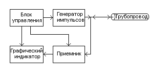
Рис.3. Упрощенная
структурная схема измерений.

    С
генератора импульсов зондирующие
импульсы подаются в трубопровод.
Отраженные импульсы поступают с
трубопровода в приемник, в котором
производятся необходимые преобразования
над ними. С выхода приемника преобразованные
сигналы поступают на графический
индикатор.     Все блоки импульсного
рефлектометра функционируют по сигналам
блока управления.     На графическом
индикаторе рефлектометра воспроизводится
рефлектограмма трубопровода — реакция
трубопровода на зондирующий импульс.

Образование
рефлектограммы трубопровода легко
проследить по диаграмме, приведенной
на рисунке 4. Здесь осью ординат является
ось расстояния, а осью абсцисс — ось
времени.

В левой
части рисунка показан трубопровод из
двух секций с согласующим устройством
и коротким замыканием, а в нижней части
— рефлектограмма этого трубопровода.
Анализируя рефлектограмму трубопровода,
оператор получает информацию о наличии
или отсутствии в ней повреждений и
неоднородностей.

Рис.4. Пример
рефлектограммы с двумя неоднородностями
в трубопроводе.

Например, по
приведенной рефлектограмме можно
сделать несколько выводов:

На рефлектограмме,
кроме зондирующего импульса, есть
только два отражения: отражение от
согласующего устройства и отражение
от короткого замыкания. Это свидетельствует
о хорошей однородности трубопровода
от начала до согласующего устройства
и от согласующего устройства до короткого
замыкания.
Выходное
сопротивление рефлектометра согласовано
с волновым сопротивлением трубопровода,
так как переотраженные сигналы, которые
при отсутствии согласования располагаются
на двойном расстоянии, отсутствуют.
Повреждение имеет
вид короткого замыкания, так как
отраженный от него сигнал изменил
полярность.
Короткое замыкание
полное, так как после отражения от него
других отражений нет.
Линия имеет большое
затухание, так как амплитуда отражения
от короткого замыкания много меньше,
чем амплитуда зондирующего сигнала.

Если
выходное сопротивление рефлектометра
не согласовано с волновым сопротивлением
трубопровода, то в моменты времени 2*
tм,
4* tм
и т.д. будут наблюдаться переотраженные
сигналы от согласующего устройства,
убывающие по амплитуде, а в моменты
времени 2*
tх,
4*tх
и т.д. — переотражения от места короткого
замыкания.

Основную
сложность и трудоемкость при методе
отраженных импульсов представляет
выделение отражения от места повреждения
на фоне помех.

Важное
значение для метода импульсной
рефлектометрии имеет отношение между
напряжением и током введенной в систему
электромагнитной волны, которое одинаково
в любой точке трубопровода. Это
соотношение:

Z
= U/I

имеет размерность
сопротивления и называется волновым
сопротивлением трубопровода.

При использовании метода импульсной
рефлектометрии в трубопроводную систему
контроля посылают зондирующий импульс
и измеряют интервал tх — время двойного
пробега этого импульса до места
повреждения (неоднородности волнового
сопротивления). Расстояние до места
повреждения рассчитывают по выражению:

Lx
= tx*V/2
,

где
V
— скорость распространения импульса в
трубопровода.

Отношение
амплитуды отраженного импульса Uо к
амплитуде зондирующего импульса Uз
обозначают коэффициентом отражения p:

p
= Uo/Uз = (Z1
— Z)
/ (Z1
+ Z),

где:
Z
— волновое сопротивление трубопровода
до места повреждения (неоднородности),

Z1
— волновое сопротивление трубопровода
в месте повреждения (неоднородности).

Отраженный
сигнал появляется в тех местах
трубопровода, где волновое сопротивление
отклоняется от своего среднего значения:
согласующие устройства, изгибах
трубопроводов, в месте обрыва, короткого
замыкания и т.д.

Если
выходное сопротивление импульсного
рефлектометра отличается от волнового
сопротивления измеряемого трубопровода,
то в месте подключения рефлектометра
к трубопровода возникают переотражения.

Переотражения
— это отражения от входного сопротивления
рефлектометра отраженных сигналов,
которые пришли к месту подключения
рефлектометра из трубопровода.

В
зависимости от соотношения входного
сопротивления рефлектометра и волнового
сопротивления трубопровода изменяется
полярность и амплитуда переотражений,
которая может оказаться соизмеримой с
амплитудой отражений. Поэтому перед
измерением рефлектометром обязательно
нужно выполнить операцию согласования
выходного сопротивления рефлектометра
с волновым сопротивлением трубопровода.

Примеры
рефлектограммы трубопровода с
переотражением без согласования
выходного сопротивления с трубопроводом
и с согласованием приведены на рис. 5 и
6:

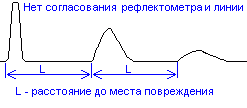
Рис.5. Рефлектограмма
трубопровода в отсутствие согласования.

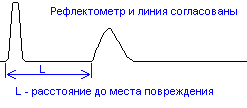
Рис.6. Рефлектограмма
трубопровода при согласовании.

При
распространении вдоль трубопровода
импульсный сигнал затухает. Затухание
трубопровода определяется ее геометрической
конструкцией и выбором материалов для
проводников и изоляции и является
частотно-зависимым. Следствием
частотной зависимости является изменение
зондирующих импульсов при их распространении
по трубопроводу: изменяется не только
амплитуда, но и форма импульса —
длительности фронта и среза импульса
увеличиваются («расплывание”
импульса). Чем длиннее трубопроводная
система, тем больше “расплывание” и
меньше амплитуда импульса. Это затрудняет
точное определение расстояния до
повреждения.

Примеры
рефлектограмм трубопроводов без
затухания и с затуханием показаны на
рисунке 7.

Рис.7. Влияние
затухания трубопровода на вид
рефлектограммы в отсутствие согласования.

Для
более точного измерения необходимо
правильно, в соответствии с длиной и
частотной характеристикой затухания
трубопровода, выбирать параметры
зондирующего импульса в рефлектометре.
Критерием правильного выбора является
минимальное «расплывание» и
максимальная амплитуда отраженного
сигнала.

Если при подключенном
трубопроводе на рефлектограмме
наблюдается только зондирующий импульс,
а отраженные сигналы отсутствуют, то
это свидетельствует о точном согласовании
выходного сопротивления рефлектометра
с волновым сопротивлением трубопровода,
отсутствии повреждений и наличии на
конце трубопровода нагрузки равной
волновому сопротивлению трубопровода
(Рис.8).

Рис.8. Рефлектограмма
при идеальном согласовании.

Вид
отраженного сигнала зависит от характера
повреждения или неоднородности. Например,
при обрыве отраженный импульс имеет ту
же полярность, что и зондирующий, а при
коротком замыкании отраженный импульс
меняет полярность (Рис.9).

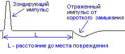
Рис.9. Рефлектограммы
при обрыве и коротком замыкании.

В
идеальном случае, когда отражение от
повреждения полное и затухание
отсутствует, амплитуда отраженного
сигнала равна амплитуде зондирующего
импульса.

Рассмотрим два
случая эквивалентных схем повреждений,
которые наиболее часто встречаются на
практике: шунтирующая
утечка
и продольное
сопротивление.

Пусть
место повреждения трубопровода
представляет собой
шунтирующую утечку
Rш:

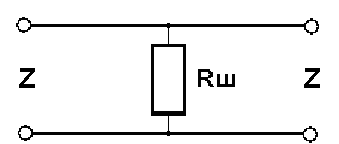
С изменением
сопротивления утечки от нуля (соответствует
короткому замыканию) до бесконечности
(соответствует исправности трубопровода),
при положительном зондирующем импульсе
отраженный импульс имеет отрицательную
полярность и изменяется по амплитуде
от максимального значения до нулевого,
в соответствии с выражением:

p=
(Z1
— Z)
/ (Z1
+ Z)
= — Z
/ (Z+2*Rш),

где:
Rш
— сопротивление шунтирующей утечки,

Z1
— волновое сопротивление трубопровода
в месте повреждения, определяется
выражением:

Z1
= (Z*R
ш) / (Z
+ Rш)

Так,
например, при коротком замыкании (Rш=0)
получаем:

p
= -1

В
этом случае сигнал отражается полностью
с изменением полярности.

При отсутствии
шунтирующей нагрузки (Rш=
)
имеем:

p
= 0

Сигнал
не отражается вообще.

При
изменении Rш
от 0 до

амплитуда отраженного сигнала уменьшается
от максимального значения до нулевого,
сохраняя отрицательную полярность (см.
рисунок).

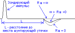
Рис.10. Рефлектограмма
при наличии шунта.

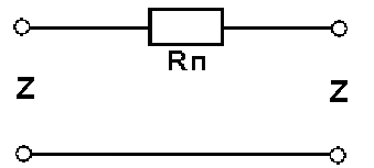
Если
эквивалентная схема места повреждения
трубопровода имеет вид включения
продольного сопротивления (например,
нарушение спайки), то с изменением
величины продольного сопротивления
отраженный импульс изменяется по
амплитуде, оставаясь той же полярности
что и зондирующий импульс.

Выражение для коэффициента отражения
при наличии включения продольного
сопротивления
будет иметь вид:

p
= (Z1
— Z)
/ (Z1
+ Z)
= 1 / (1+2*Z/Rп),

где:
Rп
— продольное сопротивление,

Z1
— волновое сопротивление трубопровода
в месте включения продольного повреждения,
определяемое выражением:

Z1
= Rп + Z

В
случае обрыва жилы (Rп=
)
получаем
коэффициент отражения:

р = 1.

Это
означает, что сигнал отражается полностью
без изменения полярности.

При нулевом
значении продольного сопротивления
(Rп=0)
имеем:

р = 0

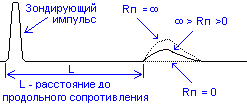
игнал
не отражается вообще.

При
изменении Rп
от

до
0 отраженный сигнал уменьшается по
амплитуде от максимального значения
до нулевого, без изменения полярности.

Рис.11. Рефлектограмма
— влияние продольного сопротивления.

Разрешающая
способность —
это минимальное расстояние между двумя
неоднородностями волнового сопротивления
при котором отраженные от них сигналы
еще наблюдаются как отдельные сигналы.

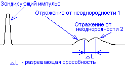
Рис.12. Рефлектограмма
— отражение от двух близких неоднородностей.

На рисунке 11
отраженные от двух неоднородностей
импульсы еще наблюдаются раздельно.

Зондирующие импульсы
распространяются в кабельных линиях
по определенным волновым каналам.

Импульсный
сигнал распространяется в трубопроводе
с определенной скоростью, которая
зависит от типа диэлектрика и определяется
выражением:

где
с
— скорость света,

g
— коэффициент укорочения электромагнитной
волны в трубопровода,

ε
— диэлектрическая проницаемость материала
изоляции трубопровода.

Коэффициент
укорочения
показывает, во сколько раз скорость
распространения импульса в трубопроводе
меньше скорости распространения в
воздухе.

В любом рефлектометре
перед измерением расстояния нужно
установить коэффициент укорочения.
Точность измерения расстояния до места
повреждения зависит от правильной
установки коэффициента укорочения.

По соотношению величин
отражения от повреждения и напряжения
помех все отражения можно разделить на
простые
и сложные.

Простое
повреждение — это такое повреждение
кабельной трубопровода, при котором
амплитуда отражения от места повреждения
больше амплитуды помех.

Сложное
повреждение — это такое повреждение,
для которого амплитуда отражения от
места повреждения меньше или равна
амплитуде помех.

По
источникам возникновения помехи бывают
асинхронные
(аддитивные)
и синхронные.

Асинхронные
помехи
не связаны с зондирующим сигналом и
неоднородностями кабельной трубопровода
и вызваны наводками от соседних кабельных
трубопроводов, от оборудования, транспорта
и различной аппаратуры.

Пример рефлектограммы трубопровода с
асинхронными помехами показан на рисунке
13.

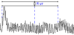
Рис.13. Рефлектограмма
трубопровода с асинхронными помехами.

На рефлектограмме
асинхронные помехи полностью закрывают
отражение от повреждения. Это отражение
невозможно рассмотреть на фоне помех.

Эффективными
методами отстройки от асинхронных помех
являются аналоговая
фильтрация
и цифровое
накопление сигнала.

Сущность цифрового
накопления
заключается в том, что одну и туже
рефлектограмму считывают несколько
раз и вычисляют среднее значение. В
связи с тем, что асинхронные помехи
носят случайный характер, после цифрового
накопления их уровень значительно
снижается.

Пример
предыдущей рефлектограммы трубопровода,
«очищенной» в результате цифрового
накопления рефлектометром, приведен
на рисунке.

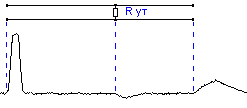
Рис.14. Рефлектограмма
с асинхронными помехами после цифровой
очистки.

На
этой рефлектограмме можно легко выделить
сигнал, отраженный от места утечки.

Синхронные
помехи связаны с зондирующим сигналом
и являются отражениями зондирующего
сигнала от неоднородностей волнового
сопротивления трубопровода (отражения
от согласующих устройств, неоднородностей
трубопроводов технологического характера
и др.).

В принципе трубопроводы
не предназначены для передачи коротких
импульсных сигналов, используемых при
методе импульсной рефлектометрии.
Поэтому этим системам контроля
трубопроводов присуще большое количество
синхронных помех. Пример рефлектограммы
трубопровода с синхронными помехами
показан на рисунке.

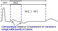
Рис.11. Рефлектограмма
трубопровода с синхронными помехами.

Синхронные
помехи можно существенно уменьшить
посредством сравнения
или
дифференциального
анализа.

При сравнении
накладывают
рефлектограммы двух трубопроводов
(неповрежденного и поврежденного),
проложенных по одной трассе.

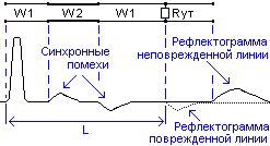
Наложение
двух рефлектограмм позволяет быстро
обнаружить начальную точку их различия,
по которой и определяют расстояние L до
повреждения.

При
дифференциальном
анализе рефлектограммы поврежденного
и неповрежденного трубопроводов
вычитают, как показано на рисунке ниже

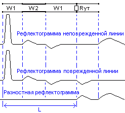
Из
рисунка видно, что при вычитании все
синхронные помехи компенсируются. По
разностной рефлектограмме легко
обнаружить отражение от места повреждения
и определить расстояние L
до него.

При
измерении качества трубопровода методом
импульсной рефлектометрии асинхронные
и синхронные помехи присутствуют на
рефлектограмме одновременно.

Асинхронные
помехи (кроме помех импульсного
характера), как правило, имеют одинаковые
величины, независимо от того, с какого
конца кабельной трубопровода ведется
измерение рефлектометром.

Синхронные
помехи при измерении с разных концов
кабеля имеют различную величину, в
зависимости от многих факторов: длины
кабельной трубопровода, затухания
импульсных сигналов, удаленности места
повреждения и мест неоднородностей
волнового сопротивления трубопровода,
точности согласования выходного
сопротивления импульсного рефлектометра
с волновым сопротивлением трубопровода
и других факторов. Поэтому отраженный
сигнал от одной и той же неоднородности
может иметь различные величины при
измерении с разных концов трубопровода.

Если
хотя бы предположительно известно, к
какому концу кабельной трубопровода
ближе может быть расположено место
повреждения, то для измерений нужно
выбирать именно этот конец кабельной
трубопровода. В других случаях желательно
проводить измерения последовательно
с двух концов трубопровода.

Следует учитывать, что даже такие
повреждения как «короткое замыкание»
и «обрыв», дающие максимальные
отражения зондирующего сигнала, не
всегда можно легко обнаружить на фоне
помех. Например, при большом затухании
и больших неоднородностях волнового
сопротивления трубопровода амплитуда
отражения от удаленного повреждений
типа “короткое замыкание” или “обрыв”
зачастую бывает меньше, чем отражения
от близко расположенных неоднородностей
волнового сопротивления. Поэтому такие
повреждения являются сложным для
обнаружения.

Соседние файлы в предмете [НЕСОРТИРОВАННОЕ]

Источник

Ошибки I и II рода при проверке гипотез, мощность

Общий обзор

Принятие неправильного решения

Мощность и связанные факторы

Проверка множественных гипотез

Общий обзор

Большинство проверяемых гипотез сравнивают между собой группы объектов, которые испытывают влияние различных факторов.

Например, можно сравнить эффективность двух видов лечения, чтобы сократить 5-летнюю смертность от рака молочной железы. Для данного исхода (например, смерть) сравнение, представляющее интерес (например, различные показатели смертности через 5 лет), называют эффектом или, если уместно, эффектом лечения.

Нулевую гипотезу выражают как отсутствие эффекта (например 5-летняя смертность от рака молочной железы одинаковая в двух группах, получающих разное лечение); двусторонняя альтернативная гипотеза будет означать, что различие эффектов не равно нулю.

Критериальная проверка гипотезы дает возможность определить, достаточно ли аргументов, чтобы отвергнуть нулевую гипотезу. Можно принять только одно из двух решений:

отвергнуть нулевую гипотезу и принять альтернативную гипотезу
остаться в рамках нулевой гипотезы

Важно: В литературе достаточно часто встречается понятие «принять нулевую гипотезу». Хотелось бы внести ясность, что со статистической точки зрения принять нулевую гипотезу невозможно, т.к. нулевая гипотеза представляет собой достаточно строгое утверждение (например, средние значения в сравниваемых группах равны ).

Поэтому фразу о принятии нулевой гипотезы следует понимать как то, что мы просто остаемся в рамках гипотезы.

Принятие неправильного решения

Возможно неправильное решение, когда отвергают/не отвергают нулевую гипотезу, потому что есть только выборочная информация.

	Верная гипотеза
H₀	H₁
Результат применения критерия	H₀	H₀ верно принята	H₀ неверно принята (Ошибка второго рода)
H₁	H₀ неверно отвергнута (Ошибка первого рода)	H₀ верно отвергнута

Ошибка 1-го рода: нулевую гипотезу отвергают, когда она истинна, и делают вывод, что имеется эффект, когда в действительности его нет. Максимальный шанс (вероятность) допустить ошибку 1-го рода обозначается α (альфа). Это уровень значимости критерия; нулевую гипотезу отвергают, если наше значение p ниже уровня значимости, т. е., если p < α.

Следует принять решение относительно значения а прежде, чем будут собраны данные; обычно назначают условное значение 0,05, хотя можно выбрать более ограничивающее значение, например 0,01.

Шанс допустить ошибку 1-го рода никогда не превысит выбранного уровня значимости, скажем α = 0,05, так как нулевую гипотезу отвергают только тогда, когда p< 0,05. Если обнаружено, что p > 0,05, то нулевую гипотезу не отвергнут и, следовательно, не допустят ошибки 1-го рода.

Ошибка 2-го рода: не отвергают нулевую гипотезу, когда она ложна, и делают вывод, что нет эффекта, тогда как в действительности он существует. Шанс возникновения ошибки 2-го рода обозначается β (бета); а величина (1-β) называется мощностью критерия.

Следовательно, мощность — это вероятность отклонения нулевой гипотезы, когда она ложна, т.е. это шанс (обычно выраженный в процентах) обнаружить реальный эффект лечения в выборке данного объема как статистически значимый.

В идеале хотелось бы, чтобы мощность критерия составляла 100%; однако это невозможно, так как всегда остается шанс, хотя и незначительный, допустить ошибку 2-го рода.

К счастью, известно, какие факторы влияют на мощность и, таким образом, можно контролировать мощность критерия, рассматривая их.

Мощность и связанные факторы

Планируя исследование, необходимо знать мощность предложенного критерия. Очевидно, можно начинать исследование, если есть «хороший» шанс обнаружить уместный эффект, если таковой существует (под «хорошим» мы подразумеваем, что мощность должна быть по крайней мере 70-80%).

Этически безответственно начинать исследование, у которого, скажем, только 40% вероятности обнаружить реальный эффект лечения; это бесполезная трата времени и денежных средств.

Ряд факторов имеют прямое отношение к мощности критерия.

Объем выборки: мощность критерия увеличивается по мере увеличения объема выборки. Это означает, что у большей выборки больше возможностей, чем у незначительной, обнаружить важный эффект, если он существует.

Когда объем выборки небольшой, у критерия может быть недостаточно мощности, чтобы обнаружить отдельный эффект. Эти методы также можно использовать для оценки мощности критерия для точно установленного объема выборки.

Вариабельность наблюдений: мощность увеличивается по мере того, как вариабельность наблюдений уменьшается.

Интересующий исследователя эффект: мощность критерия больше для более высоких эффектов. Критерий проверки гипотез имеет больше шансов обнаружить значительный реальный эффект, чем незначительный.

Уровень значимости: мощность будет больше, если уровень значимости выше (это эквивалентно увеличению допущения ошибки 1-го рода, α, а допущение ошибки 2-го рода, β, уменьшается).

Таким образом, вероятнее всего, исследователь обнаружит реальный эффект, если на стадии планирования решит, что будет рассматривать значение р как значимое, если оно скорее будет меньше 0,05, чем меньше 0,01.

Обратите внимание, что проверка ДИ для интересующего эффекта указывает на то, была ли мощность адекватной. Большой доверительный интервал следует из небольшой выборки и/или набора данных с существенной вариабельностью и указывает на недостаточную мощность.

Проверка множественных гипотез

Часто нужно выполнить критериальную проверку значимости множественных гипотез на наборе данных с многими переменными или существует более двух видов лечения.

Ошибка 1-го рода драматически увеличивается по мере увеличения числа сравнений, что приводит к ложным выводам относительно гипотез. Следовательно, следует проверить только небольшое число гипотез, выбранных для достижения первоначальной цели исследования и точно установленных априорно.

Можно использовать какую-нибудь форму апостериорного уточнения значения р, принимая во внимание число выполненных проверок гипотез.

Например, при подходе Бонферрони (его часто считают довольно консервативным) умножают каждое значение р на число выполненных проверок; тогда любые решения относительно значимости будут основываться на этом уточненном значении р.

Связанные определения:
p-уровень
Альтернативная гипотеза, альтернатива
Альфа-уровень
Бета-уровень
Гипотеза
Двусторонний критерий
Критерий для проверки гипотезы
Критическая область проверки гипотезы
Мощность
Мощность исследования
Мощность статистического критерия
Нулевая гипотеза
Односторонний критерий
Ошибка I рода
Ошибка II рода
Статистика критерия
Эквивалентные статистические критерии

В начало

Содержание портала

Источник

This article is about erroneous outcomes of statistical tests. For closely related concepts in binary classification and testing generally, see false positives and false negatives.

In statistical hypothesis testing, a type I error is the mistaken rejection of an actually true null hypothesis (also known as a «false positive» finding or conclusion; example: «an innocent person is convicted»), while a type II error is the failure to reject a null hypothesis that is actually false (also known as a «false negative» finding or conclusion; example: «a guilty person is not convicted»).^[1] Much of statistical theory revolves around the minimization of one or both of these errors, though the complete elimination of either is a statistical impossibility if the outcome is not determined by a known, observable causal process.
By selecting a low threshold (cut-off) value and modifying the alpha (α) level, the quality of the hypothesis test can be increased.^[2] The knowledge of type I errors and type II errors is widely used in medical science, biometrics and computer science.^{[clarification needed]}

Intuitively, type I errors can be thought of as errors of commission, i.e. the researcher unluckily concludes that something is the fact. For instance, consider a study where researchers compare a drug with a placebo. If the patients who are given the drug get better than the patients given the placebo by chance, it may appear that the drug is effective, but in fact the conclusion is incorrect.
In reverse, type II errors are errors of omission. In the example above, if the patients who got the drug did not get better at a higher rate than the ones who got the placebo, but this was a random fluke, that would be a type II error. The consequence of a type II error depends on the size and direction of the missed determination and the circumstances. An expensive cure for one in a million patients may be inconsequential even if it truly is a cure.

Definition[edit]

Statistical background[edit]

In statistical test theory, the notion of a statistical error is an integral part of hypothesis testing. The test goes about choosing about two competing propositions called null hypothesis, denoted by H₀ and alternative hypothesis, denoted by H₁. This is conceptually similar to the judgement in a court trial. The null hypothesis corresponds to the position of the defendant: just as he is presumed to be innocent until proven guilty, so is the null hypothesis presumed to be true until the data provide convincing evidence against it. The alternative hypothesis corresponds to the position against the defendant. Specifically, the null hypothesis also involves the absence of a difference or the absence of an association. Thus, the null hypothesis can never be that there is a difference or an association.

If the result of the test corresponds with reality, then a correct decision has been made. However, if the result of the test does not correspond with reality, then an error has occurred. There are two situations in which the decision is wrong. The null hypothesis may be true, whereas we reject H₀. On the other hand, the alternative hypothesis H₁ may be true, whereas we do not reject H₀. Two types of error are distinguished: type I error and type II error.^[3]

Type I error[edit]

The first kind of error is the mistaken rejection of a null hypothesis as the result of a test procedure. This kind of error is called a type I error (false positive) and is sometimes called an error of the first kind. In terms of the courtroom example, a type I error corresponds to convicting an innocent defendant.

Type II error[edit]

The second kind of error is the mistaken failure to reject the null hypothesis as the result of a test procedure. This sort of error is called a type II error (false negative) and is also referred to as an error of the second kind. In terms of the courtroom example, a type II error corresponds to acquitting a criminal.^[4]

Crossover error rate[edit]

The crossover error rate (CER) is the point at which type I errors and type II errors are equal. A system with a lower CER value provides more accuracy than a system with a higher CER value.

False positive and false negative[edit]

In terms of false positives and false negatives, a positive result corresponds to rejecting the null hypothesis, while a negative result corresponds to failing to reject the null hypothesis; «false» means the conclusion drawn is incorrect. Thus, a type I error is equivalent to a false positive, and a type II error is equivalent to a false negative.

Table of error types[edit]

Tabularised relations between truth/falseness of the null hypothesis and outcomes of the test:^[5]

Table of error types	Null hypothesis (H₀) is
True	False
Decision about null hypothesis (H₀)	Don’t reject	Correct inference (true negative) (probability = 1−α)	Type II error (false negative) (probability = β)
Reject	Type I error (false positive) (probability = α)	Correct inference (true positive) (probability = 1−β)

Table of error types

Null hypothesis (H₀) is

True

False

Decision
about null
hypothesis (H₀)

Don’t
reject

Correct inference
(true negative)

(probability = 1−α)

Type II error
(false negative)
(probability = β)

Reject

Type I error
(false positive)
(probability = α)

Correct inference
(true positive)

(probability = 1−β)

Error rate[edit]

The results obtained from negative sample (left curve) overlap with the results obtained from positive samples (right curve). By moving the result cutoff value (vertical bar), the rate of false positives (FP) can be decreased, at the cost of raising the number of false negatives (FN), or vice versa (TP = True Positives, TPR = True Positive Rate, FPR = False Positive Rate, TN = True Negatives).

A perfect test would have zero false positives and zero false negatives. However, statistical methods are probabilistic, and it cannot be known for certain whether statistical conclusions are correct. Whenever there is uncertainty, there is the possibility of making an error. Considering this nature of statistics science, all statistical hypothesis tests have a probability of making type I and type II errors.^[6]

The type I error rate is the probability of rejecting the null hypothesis given that it is true. The test is designed to keep the type I error rate below a prespecified bound called the significance level, usually denoted by the Greek letter α (alpha) and is also called the alpha level. Usually, the significance level is set to 0.05 (5%), implying that it is acceptable to have a 5% probability of incorrectly rejecting the true null hypothesis.^[7]
The rate of the type II error is denoted by the Greek letter β (beta) and related to the power of a test, which equals 1−β.^[8]

These two types of error rates are traded off against each other: for any given sample set, the effort to reduce one type of error generally results in increasing the other type of error.^[9]

The quality of hypothesis test[edit]

The same idea can be expressed in terms of the rate of correct results and therefore used to minimize error rates and improve the quality of hypothesis test. To reduce the probability of committing a type I error, making the alpha value more stringent is quite simple and efficient. To decrease the probability of committing a type II error, which is closely associated with analyses’ power, either increasing the test’s sample size or relaxing the alpha level could increase the analyses’ power.^[10] A test statistic is robust if the type I error rate is controlled.

Varying different threshold (cut-off) value could also be used to make the test either more specific or more sensitive, which in turn elevates the test quality. For example, imagine a medical test, in which an experimenter might measure the concentration of a certain protein in the blood sample. The experimenter could adjust the threshold (black vertical line in the figure) and people would be diagnosed as having diseases if any number is detected above this certain threshold. According to the image, changing the threshold would result in changes in false positives and false negatives, corresponding to movement on the curve.^[11]

Example[edit]

Since in a real experiment it is impossible to avoid all type I and type II errors, it is important to consider the amount of risk one is willing to take to falsely reject H₀ or accept H₀. The solution to this question would be to report the p-value or significance level α of the statistic. For example, if the p-value of a test statistic result is estimated at 0.0596, then there is a probability of 5.96% that we falsely reject H₀. Or, if we say, the statistic is performed at level α, like 0.05, then we allow to falsely reject H₀ at 5%. A significance level α of 0.05 is relatively common, but there is no general rule that fits all scenarios.

Vehicle speed measuring[edit]

The speed limit of a freeway in the United States is 120 kilometers per hour. A device is set to measure the speed of passing vehicles. Suppose that the device will conduct three measurements of the speed of a passing vehicle, recording as a random sample X₁, X₂, X₃. The traffic police will or will not fine the drivers depending on the average speed . That is to say, the test statistic

${displaystyle T={frac {X_{1}+X_{2}+X_{3}}{3}}={bar {X}}}$

In addition, we suppose that the measurements X₁, X₂, X₃ are modeled as normal distribution N(μ,4). Then, T should follow N(μ,4/3) and the parameter μ represents the true speed of passing vehicle. In this experiment, the null hypothesis H₀ and the alternative hypothesis H₁ should be

H₀: μ=120 against H₁: μ>120.

If we perform the statistic level at α=0.05, then a critical value c should be calculated to solve

${displaystyle Pleft(Zgeqslant {frac {c-120}{frac {2}{sqrt {3}}}}right)=0.05}$

According to change-of-units rule for the normal distribution. Referring to Z-table, we can get

${displaystyle {frac {c-120}{frac {2}{sqrt {3}}}}=1.645Rightarrow c=121.9}$

Here, the critical region. That is to say, if the recorded speed of a vehicle is greater than critical value 121.9, the driver will be fined. However, there are still 5% of the drivers are falsely fined since the recorded average speed is greater than 121.9 but the true speed does not pass 120, which we say, a type I error.

The type II error corresponds to the case that the true speed of a vehicle is over 120 kilometers per hour but the driver is not fined. For example, if the true speed of a vehicle μ=125, the probability that the driver is not fined can be calculated as

${displaystyle P=(T<121.9|mu =125)=Pleft({frac {T-125}{frac {2}{sqrt {3}}}}<{frac {121.9-125}{frac {2}{sqrt {3}}}}right)=phi (-2.68)=0.0036}$

which means, if the true speed of a vehicle is 125, the driver has the probability of 0.36% to avoid the fine when the statistic is performed at level 125 since the recorded average speed is lower than 121.9. If the true speed is closer to 121.9 than 125, then the probability of avoiding the fine will also be higher.

The tradeoffs between type I error and type II error should also be considered. That is, in this case, if the traffic police do not want to falsely fine innocent drivers, the level α can be set to a smaller value, like 0.01. However, if that is the case, more drivers whose true speed is over 120 kilometers per hour, like 125, would be more likely to avoid the fine.

Etymology[edit]

In 1928, Jerzy Neyman (1894–1981) and Egon Pearson (1895–1980), both eminent statisticians, discussed the problems associated with «deciding whether or not a particular sample may be judged as likely to have been randomly drawn from a certain population»:^[12] and, as Florence Nightingale David remarked, «it is necessary to remember the adjective ‘random’ [in the term ‘random sample’] should apply to the method of drawing the sample and not to the sample itself».^[13]

They identified «two sources of error», namely:

(a) the error of rejecting a hypothesis that should have not been rejected, and

(b) the error of failing to reject a hypothesis that should have been rejected.

In 1930, they elaborated on these two sources of error, remarking that:

…in testing hypotheses two considerations must be kept in view, we must be able to reduce the chance of rejecting a true hypothesis to as low a value as desired; the test must be so devised that it will reject the hypothesis tested when it is likely to be false.

In 1933, they observed that these «problems are rarely presented in such a form that we can discriminate with certainty between the true and false hypothesis» . They also noted that, in deciding whether to fail to reject, or reject a particular hypothesis amongst a «set of alternative hypotheses», H₁, H₂…, it was easy to make an error:

…[and] these errors will be of two kinds:

(I) we reject H₀ [i.e., the hypothesis to be tested] when it is true,^[14]

(II) we fail to reject H₀ when some alternative hypothesis H_A or H₁ is true. (There are various notations for the alternative).

In all of the papers co-written by Neyman and Pearson the expression H₀ always signifies «the hypothesis to be tested».

In the same paper they call these two sources of error, errors of type I and errors of type II respectively.^[15]

[edit]

Null hypothesis[edit]

It is standard practice for statisticians to conduct tests in order to determine whether or not a «speculative hypothesis» concerning the observed phenomena of the world (or its inhabitants) can be supported. The results of such testing determine whether a particular set of results agrees reasonably (or does not agree) with the speculated hypothesis.

On the basis that it is always assumed, by statistical convention, that the speculated hypothesis is wrong, and the so-called «null hypothesis» that the observed phenomena simply occur by chance (and that, as a consequence, the speculated agent has no effect) – the test will determine whether this hypothesis is right or wrong. This is why the hypothesis under test is often called the null hypothesis (most likely, coined by Fisher (1935, p. 19)), because it is this hypothesis that is to be either nullified or not nullified by the test. When the null hypothesis is nullified, it is possible to conclude that data support the «alternative hypothesis» (which is the original speculated one).

The consistent application by statisticians of Neyman and Pearson’s convention of representing «the hypothesis to be tested» (or «the hypothesis to be nullified») with the expression H₀ has led to circumstances where many understand the term «the null hypothesis» as meaning «the nil hypothesis» – a statement that the results in question have arisen through chance. This is not necessarily the case – the key restriction, as per Fisher (1966), is that «the null hypothesis must be exact, that is free from vagueness and ambiguity, because it must supply the basis of the ‘problem of distribution,’ of which the test of significance is the solution.»^[16] As a consequence of this, in experimental science the null hypothesis is generally a statement that a particular treatment has no effect; in observational science, it is that there is no difference between the value of a particular measured variable, and that of an experimental prediction.^{[citation needed]}

Statistical significance[edit]

If the probability of obtaining a result as extreme as the one obtained, supposing that the null hypothesis were true, is lower than a pre-specified cut-off probability (for example, 5%), then the result is said to be statistically significant and the null hypothesis is rejected.

British statistician Sir Ronald Aylmer Fisher (1890–1962) stressed that the «null hypothesis»:

… is never proved or established, but is possibly disproved, in the course of experimentation. Every experiment may be said to exist only in order to give the facts a chance of disproving the null hypothesis.

— Fisher, 1935, p.19

Application domains[edit]

Medicine[edit]

In the practice of medicine, the differences between the applications of screening and testing are considerable.

Medical screening[edit]

Screening involves relatively cheap tests that are given to large populations, none of whom manifest any clinical indication of disease (e.g., Pap smears).

Testing involves far more expensive, often invasive, procedures that are given only to those who manifest some clinical indication of disease, and are most often applied to confirm a suspected diagnosis.

For example, most states in the USA require newborns to be screened for phenylketonuria and hypothyroidism, among other congenital disorders.

Hypothesis: «The newborns have phenylketonuria and hypothyroidism»

Null Hypothesis (H₀): «The newborns do not have phenylketonuria and hypothyroidism»,

Type I error (false positive): The true fact is that the newborns do not have phenylketonuria and hypothyroidism but we consider they have the disorders according to the data.

Type II error (false negative): The true fact is that the newborns have phenylketonuria and hypothyroidism but we consider they do not have the disorders according to the data.

Although they display a high rate of false positives, the screening tests are considered valuable because they greatly increase the likelihood of detecting these disorders at a far earlier stage.

The simple blood tests used to screen possible blood donors for HIV and hepatitis have a significant rate of false positives; however, physicians use much more expensive and far more precise tests to determine whether a person is actually infected with either of these viruses.

Perhaps the most widely discussed false positives in medical screening come from the breast cancer screening procedure mammography. The US rate of false positive mammograms is up to 15%, the highest in world. One consequence of the high false positive rate in the US is that, in any 10-year period, half of the American women screened receive a false positive mammogram. False positive mammograms are costly, with over $100 million spent annually in the U.S. on follow-up testing and treatment. They also cause women unneeded anxiety. As a result of the high false positive rate in the US, as many as 90–95% of women who get a positive mammogram do not have the condition. The lowest rate in the world is in the Netherlands, 1%. The lowest rates are generally in Northern Europe where mammography films are read twice and a high threshold for additional testing is set (the high threshold decreases the power of the test).

The ideal population screening test would be cheap, easy to administer, and produce zero false-negatives, if possible. Such tests usually produce more false-positives, which can subsequently be sorted out by more sophisticated (and expensive) testing.

Medical testing[edit]

False negatives and false positives are significant issues in medical testing.

Hypothesis: «The patients have the specific disease».

Null hypothesis (H₀): «The patients do not have the specific disease».

Type I error (false positive): «The true fact is that the patients do not have a specific disease but the physicians judges the patients was ill according to the test reports».

False positives can also produce serious and counter-intuitive problems when the condition being searched for is rare, as in screening. If a test has a false positive rate of one in ten thousand, but only one in a million samples (or people) is a true positive, most of the positives detected by that test will be false. The probability that an observed positive result is a false positive may be calculated using Bayes’ theorem.

Type II error (false negative): «The true fact is that the disease is actually present but the test reports provide a falsely reassuring message to patients and physicians that the disease is absent».

False negatives produce serious and counter-intuitive problems, especially when the condition being searched for is common. If a test with a false negative rate of only 10% is used to test a population with a true occurrence rate of 70%, many of the negatives detected by the test will be false.

This sometimes leads to inappropriate or inadequate treatment of both the patient and their disease. A common example is relying on cardiac stress tests to detect coronary atherosclerosis, even though cardiac stress tests are known to only detect limitations of coronary artery blood flow due to advanced stenosis.

Biometrics[edit]

Biometric matching, such as for fingerprint recognition, facial recognition or iris recognition, is susceptible to type I and type II errors.

Hypothesis: «The input does not identify someone in the searched list of people»

Null hypothesis: «The input does identify someone in the searched list of people»

Type I error (false reject rate): «The true fact is that the person is someone in the searched list but the system concludes that the person is not according to the data».

Type II error (false match rate): «The true fact is that the person is not someone in the searched list but the system concludes that the person is someone whom we are looking for according to the data».

The probability of type I errors is called the «false reject rate» (FRR) or false non-match rate (FNMR), while the probability of type II errors is called the «false accept rate» (FAR) or false match rate (FMR).

If the system is designed to rarely match suspects then the probability of type II errors can be called the «false alarm rate». On the other hand, if the system is used for validation (and acceptance is the norm) then the FAR is a measure of system security, while the FRR measures user inconvenience level.

Security screening[edit]

False positives are routinely found every day in airport security screening, which are ultimately visual inspection systems. The installed security alarms are intended to prevent weapons being brought onto aircraft; yet they are often set to such high sensitivity that they alarm many times a day for minor items, such as keys, belt buckles, loose change, mobile phones, and tacks in shoes.

Here, the null hypothesis is that the item is not a weapon, while the alternative hypothesis is that the item is a weapon.

A type I error (false positive): «The true fact is that the item is not a weapon but the system still alarms».

Type II error (false negative) «The true fact is that the item is a weapon but the system keeps silent at this time».

The ratio of false positives (identifying an innocent traveler as a terrorist) to true positives (detecting a would-be terrorist) is, therefore, very high; and because almost every alarm is a false positive, the positive predictive value of these screening tests is very low.

The relative cost of false results determines the likelihood that test creators allow these events to occur. As the cost of a false negative in this scenario is extremely high (not detecting a bomb being brought onto a plane could result in hundreds of deaths) whilst the cost of a false positive is relatively low (a reasonably simple further inspection) the most appropriate test is one with a low statistical specificity but high statistical sensitivity (one that allows a high rate of false positives in return for minimal false negatives).

Computers[edit]

The notions of false positives and false negatives have a wide currency in the realm of computers and computer applications, including computer security, spam filtering, Malware, Optical character recognition and many others.

For example, in the case of spam filtering the hypothesis here is that the message is a spam.

Thus, null hypothesis: «The message is not a spam».

Type I error (false positive): «Spam filtering or spam blocking techniques wrongly classify a legitimate email message as spam and, as a result, interferes with its delivery».

While most anti-spam tactics can block or filter a high percentage of unwanted emails, doing so without creating significant false-positive results is a much more demanding task.

Type II error (false negative): «Spam email is not detected as spam, but is classified as non-spam». A low number of false negatives is an indicator of the efficiency of spam filtering.

References[edit]

^ «Type I Error and Type II Error». explorable.com. Retrieved 14 December 2019.
^ Chow, Y. W.; Pietranico, R.; Mukerji, A. (27 October 1975). «Studies of oxygen binding energy to hemoglobin molecule». Biochemical and Biophysical Research Communications. 66 (4): 1424–1431. doi:10.1016/0006-291x(75)90518-5. ISSN 0006-291X. PMID 6.
^ A modern introduction to probability and statistics : understanding why and how. Dekking, Michel, 1946-. London: Springer. 2005. ISBN 978-1-85233-896-1. OCLC 262680588.{{cite book}}: CS1 maint: others (link)
^ A modern introduction to probability and statistics : understanding why and how. Dekking, Michel, 1946-. London: Springer. 2005. ISBN 978-1-85233-896-1. OCLC 262680588.{{cite book}}: CS1 maint: others (link)
^ Sheskin, David (2004). Handbook of Parametric and Nonparametric Statistical Procedures. CRC Press. p. 54. ISBN 1584884401.
^ Smith, R. J.; Bryant, R. G. (27 October 1975). «Metal substitutions incarbonic anhydrase: a halide ion probe study». Biochemical and Biophysical Research Communications. 66 (4): 1281–1286. doi:10.1016/0006-291x(75)90498-2. ISSN 0006-291X. PMC 9650581. PMID 3.
^ Lindenmayer, David. (2005). Practical conservation biology. Burgman, Mark A. Collingwood, Vic.: CSIRO Pub. ISBN 0-643-09310-9. OCLC 65216357.
^ Chow, Y. W.; Pietranico, R.; Mukerji, A. (27 October 1975). «Studies of oxygen binding energy to hemoglobin molecule». Biochemical and Biophysical Research Communications. 66 (4): 1424–1431. doi:10.1016/0006-291x(75)90518-5. ISSN 0006-291X. PMID 6.
^ Smith, R. J.; Bryant, R. G. (27 October 1975). «Metal substitutions incarbonic anhydrase: a halide ion probe study». Biochemical and Biophysical Research Communications. 66 (4): 1281–1286. doi:10.1016/0006-291x(75)90498-2. ISSN 0006-291X. PMC 9650581. PMID 3.
^ Smith, R. J.; Bryant, R. G. (27 October 1975). «Metal substitutions incarbonic anhydrase: a halide ion probe study». Biochemical and Biophysical Research Communications. 66 (4): 1281–1286. doi:10.1016/0006-291x(75)90498-2. ISSN 0006-291X. PMC 9650581. PMID 3.
^ Moroi, K.; Sato, T. (15 August 1975). «Comparison between procaine and isocarboxazid metabolism in vitro by a liver microsomal amidase-esterase». Biochemical Pharmacology. 24 (16): 1517–1521. doi:10.1016/0006-2952(75)90029-5. ISSN 1873-2968. PMID 8.
^ NEYMAN, J.; PEARSON, E. S. (1928). «On the Use and Interpretation of Certain Test Criteria for Purposes of Statistical Inference Part I». Biometrika. 20A (1–2): 175–240. doi:10.1093/biomet/20a.1-2.175. ISSN 0006-3444.
^ C.I.K.F. (July 1951). «Probability Theory for Statistical Methods. By F. N. David. [Pp. ix + 230. Cambridge University Press. 1949. Price 155.]». Journal of the Staple Inn Actuarial Society. 10 (3): 243–244. doi:10.1017/s0020269x00004564. ISSN 0020-269X.
^ Note that the subscript in the expression H₀ is a zero (indicating null), and is not an «O» (indicating original).
^ Neyman, J.; Pearson, E. S. (30 October 1933). «The testing of statistical hypotheses in relation to probabilities a priori». Mathematical Proceedings of the Cambridge Philosophical Society. 29 (4): 492–510. Bibcode:1933PCPS…29..492N. doi:10.1017/s030500410001152x. ISSN 0305-0041. S2CID 119855116.
^ Fisher, R.A. (1966). The design of experiments. 8th edition. Hafner:Edinburgh.

Bibliography[edit]

Betz, M.A. & Gabriel, K.R., «Type IV Errors and Analysis of Simple Effects», Journal of Educational Statistics, Vol.3, No.2, (Summer 1978), pp. 121–144.
David, F.N., «A Power Function for Tests of Randomness in a Sequence of Alternatives», Biometrika, Vol.34, Nos.3/4, (December 1947), pp. 335–339.
Fisher, R.A., The Design of Experiments, Oliver & Boyd (Edinburgh), 1935.
Gambrill, W., «False Positives on Newborns’ Disease Tests Worry Parents», Health Day, (5 June 2006). [1] Archived 17 May 2018 at the Wayback Machine
Kaiser, H.F., «Directional Statistical Decisions», Psychological Review, Vol.67, No.3, (May 1960), pp. 160–167.
Kimball, A.W., «Errors of the Third Kind in Statistical Consulting», Journal of the American Statistical Association, Vol.52, No.278, (June 1957), pp. 133–142.
Lubin, A., «The Interpretation of Significant Interaction», Educational and Psychological Measurement, Vol.21, No.4, (Winter 1961), pp. 807–817.
Marascuilo, L.A. & Levin, J.R., «Appropriate Post Hoc Comparisons for Interaction and nested Hypotheses in Analysis of Variance Designs: The Elimination of Type-IV Errors», American Educational Research Journal, Vol.7., No.3, (May 1970), pp. 397–421.
Mitroff, I.I. & Featheringham, T.R., «On Systemic Problem Solving and the Error of the Third Kind», Behavioral Science, Vol.19, No.6, (November 1974), pp. 383–393.
Mosteller, F., «A k-Sample Slippage Test for an Extreme Population», The Annals of Mathematical Statistics, Vol.19, No.1, (March 1948), pp. 58–65.
Moulton, R.T., «Network Security», Datamation, Vol.29, No.7, (July 1983), pp. 121–127.
Raiffa, H., Decision Analysis: Introductory Lectures on Choices Under Uncertainty, Addison–Wesley, (Reading), 1968.

External links[edit]

Bias and Confounding – presentation by Nigel Paneth, Graduate School of Public Health, University of Pittsburgh

Источник

This article is about erroneous outcomes of statistical tests. For closely related concepts in binary classification and testing generally, see false positives and false negatives.