Packet error rate это - Исправление ошибок и поиск оптимальных решений проблем

From Wikipedia, the free encyclopedia

In digital transmission, the number of bit errors is the number of received bits of a data stream over a communication channel that have been altered due to noise, interference, distortion or bit synchronization errors.

The bit error rate (BER) is the number of bit errors per unit time. The bit error ratio (also BER) is the number of bit errors divided by the total number of transferred bits during a studied time interval. Bit error ratio is a unitless performance measure, often expressed as a percentage.^[1]

The bit error probability p_e is the expected value of the bit error ratio. The bit error ratio can be considered as an approximate estimate of the bit error probability. This estimate is accurate for a long time interval and a high number of bit errors.

Example[edit]

As an example, assume this transmitted bit sequence:

1 1 0 0 0 1 0 1 1

and the following received bit sequence:

0 1 0 1 0 1 0 0 1,

The number of bit errors (the underlined bits) is, in this case, 3. The BER is 3 incorrect bits divided by 9 transferred bits, resulting in a BER of 0.333 or 33.3%.

Packet error ratio[edit]

The packet error ratio (PER) is the number of incorrectly received data packets divided by the total number of received packets. A packet is declared incorrect if at least one bit is erroneous. The expectation value of the PER is denoted packet error probability p_p, which for a data packet length of N bits can be expressed as

${displaystyle p_{p}=1-(1-p_{e})^{N}=1-e^{Nln(1-p_{e})}}$

assuming that the bit errors are independent of each other. For small bit error probabilities and large data packets, this is approximately

$p_{p}approx p_{e}N.$

Similar measurements can be carried out for the transmission of frames, blocks, or symbols.

The above expression can be rearranged to express the corresponding BER (p_e) as a function of the PER (p_p) and the data packet length N in bits:

${displaystyle p_{e}=1-{sqrt[{N}]{(1-p_{p})}}}$

Factors affecting the BER[edit]

In a communication system, the receiver side BER may be affected by transmission channel noise, interference, distortion, bit synchronization problems, attenuation, wireless multipath fading, etc.

The BER may be improved by choosing a strong signal strength (unless this causes cross-talk and more bit errors), by choosing a slow and robust modulation scheme or line coding scheme, and by applying channel coding schemes such as redundant forward error correction codes.

The transmission BER is the number of detected bits that are incorrect before error correction, divided by the total number of transferred bits (including redundant error codes). The information BER, approximately equal to the decoding error probability, is the number of decoded bits that remain incorrect after the error correction, divided by the total number of decoded bits (the useful information). Normally the transmission BER is larger than the information BER. The information BER is affected by the strength of the forward error correction code.

Analysis of the BER[edit]

The BER may be evaluated using stochastic (Monte Carlo) computer simulations. If a simple transmission channel model and data source model is assumed, the BER may also be calculated analytically. An example of such a data source model is the Bernoulli source.

Examples of simple channel models used in information theory are:

Binary symmetric channel (used in analysis of decoding error probability in case of non-bursty bit errors on the transmission channel)
Additive white Gaussian noise (AWGN) channel without fading.

A worst-case scenario is a completely random channel, where noise totally dominates over the useful signal. This results in a transmission BER of 50% (provided that a Bernoulli binary data source and a binary symmetrical channel are assumed, see below).

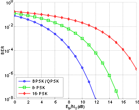
Bit-error rate curves for BPSK, QPSK, 8-PSK and 16-PSK, AWGN channel.

In a noisy channel, the BER is often expressed as a function of the normalized carrier-to-noise ratio measure denoted Eb/N0, (energy per bit to noise power spectral density ratio), or Es/N0 (energy per modulation symbol to noise spectral density).

For example, in the case of QPSK modulation and AWGN channel, the BER as function of the Eb/N0 is given by:
$operatorname {BER}={frac {1}{2}}operatorname {erfc}({sqrt {E_{b}/N_{0}}})$ .^[2]

People usually plot the BER curves to describe the performance of a digital communication system. In optical communication, BER(dB) vs. Received Power(dBm) is usually used; while in wireless communication, BER(dB) vs. SNR(dB) is used.

Measuring the bit error ratio helps people choose the appropriate forward error correction codes. Since most such codes correct only bit-flips, but not bit-insertions or bit-deletions, the Hamming distance metric is the appropriate way to measure the number of bit errors. Many FEC coders also continuously measure the current BER.

A more general way of measuring the number of bit errors is the Levenshtein distance.
The Levenshtein distance measurement is more appropriate for measuring raw channel performance before frame synchronization, and when using error correction codes designed to correct bit-insertions and bit-deletions, such as Marker Codes and Watermark Codes.^[3]

Mathematical draft[edit]

The BER is the likelihood of a bit misinterpretation due to electrical noise w(t) . Considering a bipolar NRZ transmission, we have

$x_{1}(t)=A+w(t)$ for a «1» and $x_{0}(t)=-A+w(t)$ for a «0». Each of $x_{1}(t)$ and x_0(t) has a period of .

Knowing that the noise has a bilateral spectral density ${frac {N_{0}}{2}}$ ,

$x_{1}(t)$ is ${mathcal {N}}left(A,{frac {N_{0}}{2T}}right)$

and x_0(t) is ${mathcal {N}}left(-A,{frac {N_{0}}{2T}}right)$ .

Returning to BER, we have the likelihood of a bit misinterpretation $p_{e}=p(0|1)p_{1}+p(1|0)p_{0}$ .

$p(1|0)=0.5,operatorname {erfc}left({frac {A+lambda }{{sqrt {N_{o}/T}}}}right)$ and $p(0|1)=0.5,operatorname {erfc}left({frac {A-lambda }{{sqrt {N_{o}/T}}}}right)$

where lambda is the threshold of decision, set to 0 when $p_{1}=p_{0}=0.5$ .

We can use the average energy of the signal $E=A^{2}T$ to find the final expression :

$p_{e}=0.5,operatorname {erfc}left({sqrt {{frac {E}{N_{o}}}}}right).$
±§

Bit error rate test[edit]

BERT or bit error rate test is a testing method for digital communication circuits that uses predetermined stress patterns consisting of a sequence of logical ones and zeros generated by a test pattern generator.

A BERT typically consists of a test pattern generator and a receiver that can be set to the same pattern. They can be used in pairs, with one at either end of a transmission link, or singularly at one end with a loopback at the remote end. BERTs are typically stand-alone specialised instruments, but can be personal computer–based. In use, the number of errors, if any, are counted and presented as a ratio such as 1 in 1,000,000, or 1 in 1e06.

Common types of BERT stress patterns[edit]

PRBS (pseudorandom binary sequence) – A pseudorandom binary sequencer of N Bits. These pattern sequences are used to measure jitter and eye mask of TX-Data in electrical and optical data links.
QRSS (quasi random signal source) – A pseudorandom binary sequencer which generates every combination of a 20-bit word, repeats every 1,048,575 words, and suppresses consecutive zeros to no more than 14. It contains high-density sequences, low-density sequences, and sequences that change from low to high and vice versa. This pattern is also the standard pattern used to measure jitter.
3 in 24 – Pattern contains the longest string of consecutive zeros (15) with the lowest ones density (12.5%). This pattern simultaneously stresses minimum ones density and the maximum number of consecutive zeros. The D4 frame format of 3 in 24 may cause a D4 yellow alarm for frame circuits depending on the alignment of one bits to a frame.
1:7 – Also referred to as 1 in 8. It has only a single one in an eight-bit repeating sequence. This pattern stresses the minimum ones density of 12.5% and should be used when testing facilities set for B8ZS coding as the 3 in 24 pattern increases to 29.5% when converted to B8ZS.
Min/max – Pattern rapid sequence changes from low density to high density. Most useful when stressing the repeater’s ALBO feature.
All ones (or mark) – A pattern composed of ones only. This pattern causes the repeater to consume the maximum amount of power. If DC to the repeater is regulated properly, the repeater will have no trouble transmitting the long ones sequence. This pattern should be used when measuring span power regulation. An unframed all ones pattern is used to indicate an AIS (also known as a blue alarm).
All zeros – A pattern composed of zeros only. It is effective in finding equipment misoptioned for AMI, such as fiber/radio multiplex low-speed inputs.
Alternating 0s and 1s — A pattern composed of alternating ones and zeroes.
2 in 8 – Pattern contains a maximum of four consecutive zeros. It will not invoke a B8ZS sequence because eight consecutive zeros are required to cause a B8ZS substitution. The pattern is effective in finding equipment misoptioned for B8ZS.
Bridgetap — Bridge taps within a span can be detected by employing a number of test patterns with a variety of ones and zeros densities. This test generates 21 test patterns and runs for 15 minutes. If a signal error occurs, the span may have one or more bridge taps. This pattern is only effective for T1 spans that transmit the signal raw. Modulation used in HDSL spans negates the bridgetap patterns’ ability to uncover bridge taps.
Multipat — This test generates five commonly used test patterns to allow DS1 span testing without having to select each test pattern individually. Patterns are: all ones, 1:7, 2 in 8, 3 in 24, and QRSS.
T1-DALY and 55 OCTET — Each of these patterns contain fifty-five (55), eight bit octets of data in a sequence that changes rapidly between low and high density. These patterns are used primarily to stress the ALBO and equalizer circuitry but they will also stress timing recovery. 55 OCTET has fifteen (15) consecutive zeroes and can only be used unframed without violating one’s density requirements. For framed signals, the T1-DALY pattern should be used. Both patterns will force a B8ZS code in circuits optioned for B8ZS.

Bit error rate tester[edit]

A bit error rate tester (BERT), also known as a «bit error ratio tester»^[4] or bit error rate test solution (BERTs) is electronic test equipment used to test the quality of signal transmission of single components or complete systems.

The main building blocks of a BERT are:

Pattern generator, which transmits a defined test pattern to the DUT or test system
Error detector connected to the DUT or test system, to count the errors generated by the DUT or test system
Clock signal generator to synchronize the pattern generator and the error detector
Digital communication analyser is optional to display the transmitted or received signal
Electrical-optical converter and optical-electrical converter for testing optical communication signals

References[edit]

^ Jit Lim (14 December 2010). «Is BER the bit error ratio or the bit error rate?». EDN. Retrieved 2015-02-16.
^
Digital Communications, John Proakis, Massoud Salehi, McGraw-Hill Education, Nov 6, 2007
^
«Keyboards and Covert Channels»
by Gaurav Shah, Andres Molina, and Matt Blaze (2006?)
^ «Bit Error Rate Testing: BER Test BERT » Electronics Notes». www.electronics-notes.com. Retrieved 2020-04-11.

This article incorporates public domain material from Federal Standard 1037C. General Services Administration. (in support of MIL-STD-188).

External links[edit]

QPSK BER for AWGN channel – online experiment

Источник

Delay-tolerant networks (DTNs) for satellite communications

C. Caini, in Advances in Delay-Tolerant Networks (DTNs) (Second Edition), 2021

2.3.4.4 PER and congestion

This environment suffers from congestion and PER simultaneously. Results are close to the congestion-only case, which shows that congestion is the dominant impairment.

Results of Fig. 2.3 prove the essential equivalence of DTN and PEP performance in the presence of continuous links, i.e., for fixed terminals, which is a fundamental result. It shows that DTN can provide the same goodput performance as the most effective and widely adopted solutions even in the absence of disruptions and/or network partitioning. The challenge here is the long RTT of the GEO satellite, which is enough to justify the adoption of DTN.

Read full chapter

URL:

https://www.sciencedirect.com/science/article/pii/B9780081027936000023

Transceiver Requirements

Shahin Farahani, in ZigBee Wireless Networks and Transceivers, 2008

4.2 Receiver Sensitivity

In the IEEE 802.15.4 standard, receiver sensitivity is defined as the lowest received signal power that yields a packet error rate (PER) of less than 1% [2]. IEEE 802.15.4 requires only −85 dBm of sensitivity for operations in the 2.4 GHz ISM band. In the 868/915 MHz band, if the BPSK modulation is used, the required sensitivity is −92 dBm. The optional modes of operation in the 868/915 MHz band (using ASK and OQPSK modulation) must meet −85 dBm of sensitivity.

If a 50 Ohm single-ended antenna is used, the sensitivity level of −85 dBm translates to a signal with effective (or rms) voltage of 12.6 uV:

Signal power=-85dBm=10(-85-3010)=3.16×10-12=3.16pW

Signal voltage=P×R=3.16×10-12×50=12.6uV

This means that any received signal with root-mean-square (rms) voltage of 12.6 uV or higher can be detected and the data can be extracted with a PER of less than 1%. During this test, no interference (Section 4.3) is present. Also, the PHY Service Data Unit (PSDU) length of the data packets used in this test must be 20 octets. Although it’s not required by the standard, the available commercial transceivers are capable of delivering −95 dBm to −100 dBm of sensitivity level.

Based on IEEE 802.15.4, receiver sensitivity is measured with a signal that has 0% error vector magnitude (EVM), whereas in reality, the signal may have an EVM of up to 35%, which is the maximum EVM allowed in IEEE 802.15.4. The EVM, discussed in Section 4.7, is an indication of the modulation inaccuracy. The EVM can worsen the sensitivity level, but as long as the EVM is below 35%, the sensitivity degradation should be less than 2 dB.

In IEEE 802.15.4, the carrier frequency offset of the input signal is zero during the receiver sensitivity test [2]. In reality, however, the input signal has some frequency offset and if the receiver does not use a frequency offset correction mechanism, the sensitivity level will be degraded. Figure 4.2 shows an example of receiver sensitivity degradation versus input carrier frequency offset when there is no offset correction.

Figure 4.2. Example of Receiver Sensitivity Degradation due to frequency offset

IEEE 802.15.4 not only defines the receiver minimum input signal lever (receiver sensitivity), it also determines the receiver maximum input level. A receiver must be able to receive signals with a power level of −20 dBm or higher and maintain PER of less than 1% to be compliant with IEEE 802.1.5.4.

Read full chapter

URL:

https://www.sciencedirect.com/science/article/pii/B9780750683937000042

Wireless Local Area Networks

Vijay K. Garg, in Wireless Communications & Networking, 2007

21.12.2 PER from M Neighboring IEEE 802.11 WLANs^*

Under IEEE 802.11 FH, the probability of M IEEE 802.11 induced collisions on a Bluetooth packet is given as [17]:

(21.4)PER=1−{[1−|G|L]⋅(7879)⌈H/L⌉+|G|L⋅(5779)⌈H/L⌉−G/|G|}M

Under IEEE 802.11 DS, the probability of M IEEE 802.11 induced collisions on a Bluetooth packet is given as:

(21.5)PER=1−{[1−|G|L]⋅(5779)⌈H/L⌉+|G|L⋅(5779)⌈H/L⌉−G/|G|}M

where:

H = the duration of a Bluetooth packet

L = the dwell period of an IEEE 802.11 transmission

T_w = the packet duration of IEEE 802.11

G = ⌈H/L⌉L−Tw−H

⌈x⌉ = the least integer greater than or equal to x

The collision probability of a Bluetooth piconet where there are N neighboring Bluetooth piconets and M IEEE 802.11 WLANs will be:

(21.6)(PER)syn=1−[(7879)N⋅(Ps)M]

(21.7)(PER)asyn=1−(PsUR)N(Ps)M

Read full chapter

URL:

https://www.sciencedirect.com/science/article/pii/B9780123735805500557

Physical layer design

Husheng Li, in Communications for Control in Cyber Physical Systems, 2016

8.5.1 Motivation

Since the reliability of communication is usually very high in CPSs (e.g., in the wide area monitoring system in smart grids, the packet error rate should be less than 10⁻⁵ [166]) while the communication channel may experience various degradations (e.g., the harsh environments for communications in smart grids), it is important to use channel coding to protect the information transmission.

A straightforward approach for coding in a CPS is to follow the traditional procedure of separate quantization, coding, transmission, decoding, and further processing, which is adopted in conventional communication systems (Fig. 8.7). However, separate channel decoding and system state estimation may not be optimal when there exist redundancies in the transmitted messages. For example, the transmitted codeword at time t, b(t), is generated by the observation on the physical dynamics, y(t). Due to the time correlation of system states, y(t) is correlated with y(t + 1), thus being able to provide information for decoding the codeword in the next time slot t + 1. Hence if the decoding procedure is independent of the system state estimation, the permanence will be degraded due to the loss of redundancy. One may argue that the redundancy can be removed in the source coding procedure (e.g., encoding only the innovation vector in Kalman filtering if the physical dynamics is linear with Gaussian noise [167]). However, this requires substantial computation, which a sensor may not be able to carry out. Moreover, the sensor may not have the overall system parameters for the extraction of innovation information. Hence it is more desirable to shift the burden to the controller, which has more computational power and more system information; then the inexpensive sensor focuses on transmitting the raw data.

Fig. 8.7. Illustration of the components in a CPS.

In this section, we propose an algorithm for joint channel decoding and state estimation in a CPS. We consider traditional channel codes with memory (e.g., convolutional codes). Then the physical dynamics system state evolution and the channel codes can be considered as an equivalent concatenated code, as illustrated in Fig. 8.8, in which the outer code is the generation of system observation (we call it a “nature encoded” codeword) while the inner code is the traditional channel coding. The outer code is generated by the physical dynamics in an analog manner (since the value is continuous) while the inner code is carried out by a digital encoder. We will use belief propagation (BP) [168], which has been widely applied in decoding turbo codes and low-density parity-check (LDPC) codes, to decode this equivalent concatenated code. The major challenge is that the Bayesian inference is over a hybrid system which has both continuous- and discrete-valued nodes.

Fig. 8.8. Illustration of the equivalent concatenated code for system state evolution and channel coding.

Read full chapter

URL:

https://www.sciencedirect.com/science/article/pii/B9780128019504000081

Radio channel access challenges in LoRa low-power wide-area networks

Congduc Pham, … Muhammad Ehsan, in LPWAN Technologies for IoT and M2M Applications, 2020

4.2.1.1 Encoding

First, the binary source input bits pass through an encoder. The output of encoder depends on the choice of CR value. Encoding reduces the packet error rate in the presence of short bursts of interference. LoRa uses Hamming codes for FEC. These are linear block codes and are easy to implement. LoRa uses coding rates CR of 4/5, 2/3, 4/7, and 1/2, which means if the code rate is denoted as k/n, where k represents the number of useful information bits, and encoder generates n output bits, then (n−k) are the redundant bits. If we assume CR values between 1, 2, 3, and 4 for coding rates 4/5, 4/6, 4/7, and 4/8, respectively, then the error detection and correction capabilities are as shown in Table 4–1.

Table 4–1. Error detection and correction capabilities of LoRa.

Coding rates	Error detection (bits)	Error correction (bits)
4/5	0	0
4/6	1	0
4/7	2	1
4/8	3	1

Read full chapter

URL:

https://www.sciencedirect.com/science/article/pii/B9780128188804000041

LoRaWAN for smart cities: experimental study in a campus deployment

Rakshit Ramesh, … Bharadwaj Amrutur, in LPWAN Technologies for IoT and M2M Applications, 2020

15.3.1.4 Range and packet error rate for SF8–SF11

For the sake of brevity, we have only shown results of SF12 and SF7. Our experiments show that the range of network gradually increases with increase in SF and the PER for peripheral regions in each SF becomes smaller. In SF11 (comparing with Fig. 15–4), it is observed that region (G) is not covered by the network and region € experiences a PER of >80%. In SF8 (comparing with Fig. 15–3), it is observed that region (D) comes under the network coverage and PER of region C decreases to <80%. Likewise, the trends for SF9 and SF10 become increasingly better.

Read full chapter

URL:

https://www.sciencedirect.com/science/article/pii/B9780128188804000168

Long-term evolution for machines (LTE-M)

Suresh R. Borkar, in LPWAN Technologies for IoT and M2M Applications, 2020

7.3.6 Use of LTE priority structure for LTE-M applications

One of the distinctive features of LTE is the very versatile and robust priority assignment structure for user-traffic bearers. There are 13 priority levels ranging from 0.5 (highest) to 9 (lowest) supporting guaranteed bit–rate (GBR) and non-GBR (N-GBR) bearers [20]. The priority levels are characterized by varying combinations of packet delay and packet error rate (PER). Packet delays range from 50 to 300 milliseconds and a range of 10⁻² to 10⁻⁶ is available for PER. The standards provide suggested mapping of various application classes to these priority levels but the network operators can apply their own discretion to assign the priority levels for their services. This is a strong and effective platform for managing the varying quality of service (QoS) requirements for LTE-M-based LPWAN services and provides a unique advantage to LTE-M.

Several classes of applications can be mapped for LTE-M usage. A representative mapping is suggested in Table 7–1. The best available PER of 10⁻⁶ is used since data integrity is very important for MTC type applications. This is paired with three options for packet delay—60, 100, and 300 milliseconds.

Table 7–1. Proposed LTE-M priority structure.

3GPP suggested service	Priority level	Est. packet delay (milliseconds)	Est. packet error rate	Suggested LTE-M application
Nonconversational video	5 (GBR)	300	10⁻⁶	MTC 1
IMS signaling	1 (N-GBR)	100	10⁻⁶	MTC 2
Mission-critical delay-sensitive signaling	0.5 (N-GBR)	60	10⁻⁶	MTC 3

MTC1 are applications, which may be delay-tolerant, for example utility meters. MTC 3 type applications may be delay-sensitive, for example remote robotics surgery. MTC 2 can be applied to applications such as smart city which fall in between these two extreme attributes.

Read full chapter

URL:

https://www.sciencedirect.com/science/article/pii/B9780128188804000077

Quality of service control

Yali Guo, Tricci So, in 5G NR and Enhancements, 2022

13.5.2 Alternative quality of service profile

The QoS notification control mechanism can solve the problem of service interruption due to the bearer release when the QoS cannot be guaranteed. The 5G–AN sends the notification to the core network that the QoS cannot be guaranteed. But the interaction between the core network and the application is slow. Hence, it is uncertain whether or not the application will adjust the QoS requirements. The 5G–AN can only allocate resources to meet the original QoS requirements while waiting for the adjustment instructions from the core network. At this point, the allocation of resources by the 5G–AN could become unsustainable. Due to such consideration, the alternative QoS profile is introduced as part of the QoS notification control mechanism in the 5G system. Such QoS profile is used to make the 5G–AN aware of the alternative QoS profiles when the original QoS cannot be guaranteed, so as to further improve the efficiency of resource allocation.

An alternative QoS profile is an optional optimization that depends on the QoS notification control mechanism and is only used for GBR QoS Flows with QoS notification control enabled. The PCF provides one or more alternative QoS parameter sets in the PCC rules by interacting with the AF. Then the SMF generates one or more QoS profiles for the corresponding QoS Flow, and sends them to the 5G–AN.

When the QoS cannot be guaranteed, the 5G–AN evaluates whether the resources can be sustained by one of the alternative QoS profiles. If so, it will indicate the alternative QoS profile that can be guaranteed when sending notification to the SMF. The operation at the 5G–AN is as follows:

1.: When the GFBR, PDB, or PER of a QoS Flow cannot be guaranteed, the 5G–AN evaluates whether the radio resources can guarantee an alternative QoS profile one by one according to the priority of the alternative QoS profiles. If an alternative QoS profile can be guaranteed, the 5G–AN indicates to the SMF the first matched alternative QoS profile. If none of the alternative QoS profiles can be guaranteed, the 5G–AN indicates to the SMF that QoS requirements cannot be guaranteed and there is no viable alternative QoS profile.
2.: After that, when the 5G–AN determines that the currently fulfilled GFBR, PDB, or PER are different (better or worse) from the situation indicated in the last notification, the 5G–AN indicates the latest QoS status to the SMF again.
3.: The 5G–AN always tries to fulfill the QoS profile with any alternative QoS profile that has the highest priority to meet the current situation.
4.: The SMF needs to notify the PCF after receiving the notification from the 5G–AN.
5.: The SMF may also inform the UE about changes in the QoS parameters.

Read full chapter

URL:

https://www.sciencedirect.com/science/article/pii/B9780323910606000131

LoRaWAN protocol: specifications, security, and capabilities

Alper Yegin, … Nicolas Sornin, in LPWAN Technologies for IoT and M2M Applications, 2020

3.3.3 LoRaWAN network capacity and scaling

The Okumura–Hata model is the radio propagation model to simulate results as pictured in Fig. 3–6. It is valid for deployments for which the base station is installed at high outdoor locations compared to the height of surrounding buildings. Devices are assumed to have a 0 dBi antenna, which is typical for small devices. Our simulation uses 16 channels and targets a 10% packet error rate. Fig. 3–6 shows the random position of devices and color coding for their optimal spreading factor in a hexagonal network.

Figure 3–6. Simulated network layout with hexagonal tiling.

Fig. 3–7 shows the maximum capacity results for the network and a single cell. It confirms that capacity scales easily with the density of network gateways.

Figure 3–7. Impact of multicell deployment on capacity.

These results show that the future of LoRaWAN networks, particularly in urban environments where the noise floor is expected to rise due to increased traffic, is going toward microcellular networks, for example, with receivers integrated in triple-play modems. Macro-diversity provides not only higher capacity, see Fig. 3–8, but also greater resilience to interference and lower power consumption for end devices.

Figure 3–8. Evolution of capacity as intersite distance (ISD) becomes shorter (number of messages (in millions) vs ISD).

LoRaWAN provides a horizontal connectivity solution to address the wide-ranging needs of IoT applications for LPWAN deployments. However, these benefits are only possible with intelligent NS algorithms proprietary to network solution vendors.

Read full chapter

URL:

https://www.sciencedirect.com/science/article/pii/B978012818880400003X

Performance of IEEE 802.16m and 3GPP LTE-Advanced

Sassan Ahmadi, in Mobile WiMAX, 2011

12.9.7 IEEE 802.16m Link Budget

The IMT-Advanced submissions were required to provide a detailed link budget analysis under the ITU-R specified test environments. Report ITU-R M.2135-1 provided a methodology and common parameters in order to calculate the downlink and uplink link budgets. In addition to the common parameters, the following assumptions were made in the calculations:

•: There are four transmit antennas and four receive antennas in the BS, and there are two transmit antennas and two 2 receive antennas in the MS.
•: The target packet error rate is 10% for initial transmission of data channels, and 1% for the control channels.
•: The modulation and coding scheme for the DL Assignment A-MAP is QPSK 1/8.
•: There are 6 bits transmitted over the uplink primary fast-feedback channel.
•: The MIMO scheme for downlink data is rank-1 wideband beamforming, for downlink control is SFBC with non-adaptive precoder, for uplink data is rank-1 wideband beamforming, and for uplink control is single antenna transmission.
•: The permutation (subchannelization) scheme used for DL/UL data is mini-band CRU and for DL control is DRU.
•: There is 2 dB pilot-boosting over data tones in the downlink, and no pilot boosting in the uplink.
•: No HARQ is assumed for the control channel.
•: 0.5 dB HARQ combining gain for the data channel.

Shadowing fade margin is determined as a function of the cell edge coverage reliability and the standard deviation of the log-normal shadow-fading, including penetration loss. Cell edge coverage reliability is determined for the given area coverage reliability as a function of the shadow fading standard deviation and the path loss exponent obtained from the path loss model. The cell edge reliability can be determined using simulations or using traditional numerical methods. Cell area reliability is defined as the percentage of the cell area over which coverage can be guaranteed. It is obtained from the cell edge reliability, shadow fading standard deviation, and the path loss exponent. The latter two values are used to calculate a fade margin. Macro diversity gain may be considered explicitly in order to improve the system margin or implicitly by reducing the fade margin. The path loss models are summarized in Table A1-2 of Report ITU-R M.2135-1 [6]. The IEEE 802.16m link budget in the downlink and uplink under various deployment scenarios for the TDD mode is given in Table 12-17.

TABLE 12-17. IEEE 802.16m Link Budget in Various Test Environments for the TDD Duplex Scheme [2]

	InH	UMi	UMa	RMa
Parameter	Downlink	Uplink	Downlink	Uplink	Downlink	Uplink	Downlink	Uplink
System Configuration
Carrier Frequency (GHz)	3.4	3.4	2.5	2.5	2	2	0.8	0.8
BS Antenna Heights (m)	6	6	10	10	25	25	35	35
MS Antenna Heights (m)	1.5	1.5	1.5	1.5	1.5	1.5	1.5	1.5
Cell Area Reliability	95%	95%	95%	95%	95%	95%	95%	95%
Transmission Bit Rate for Control Channel (kbps)	89.6	1.2	89.6	1.2	89.6	1.2	89.6	1.2
Transmission Bit Rate for Data Channel (Mbps)	20.23	0.98	7.53	0.21	7.53	0.21	7.53	0.21
Target Packet Error Rate for Control Channels	10⁻²	10⁻²	10⁻²	10⁻²	10⁻²	10⁻²	10⁻²	10⁻²
Target Packet Error Rate for Data Channels	10⁻¹	10⁻¹	10⁻¹	10⁻¹	10⁻¹	10⁻¹	10⁻¹	10⁻¹
Spectral Efficiency (bits/s/Hz) for Data	0.856	0.830	0.637	0.720	0.637	0.720	0.637	0.720
Pathloss Model	NLoS	NLoS	NLoS	NLoS	NLoS	NLoS	NLoS	NLoS
Mobile Speed (km/h)	3	3	3	3	30	30	120	120
Feeder Loss (dB)	2	2	2	2	2	2	2	2
Transmitter
Number of Transmit Antennas	4	2	4	2	4	2	4	2
Maximum Transmit Power per Antenna (dBm)	18	18	38	21	43	21	43	21
Total Transmit Power (dBm)	24	21	44	24	49	24	49	24
Transmitter Antenna Gain (dBi)	0	0	17	0	17	0	17	0
Transmitter Array Gain (dB)	0	0	0	0	0	0	0	0
Control Channel Power Boosting Gain (dB)	0	0	0	0	0	0	0	0
Data Channel Power Loss Due to Pilot/Control Boosting (dB)	0.2734	0	0.2734	0	0.2734	0	0.2734	0
Cable, Connector, Combiner, Body Losses, etc. (dB)	3	1	3	1	3	1	3	1
Control Channel EIRP (dBm)	21	20	58	23	63	23	63	23
Data Channel EIRP (dBm)	20.73	20	57.73	23	62.73	23	62.73	23
Receiver
Number of Receive Antennas	2	4	2	4	2	4	2	4
Receiver Antenna Gain (dBi)	0	0	0	17	0	17	0	17
Cable, Connector, Combiner, Body Losses, etc. (dB)	1	3	1	3	1	3	1	3
Receiver Noise Figure (dB)	7	5	7	5	7	5	7	5
Thermal Noise Density (dBm/Hz)	−174	−174	−174	−174	−174	−174	−174	−174
Receiver Interference Density (dBm/Hz)	−174	−174	−165	−166	−165	−166	−165	−166
Total Noise Plus Interference Density (dBm/Hz)	−166.21	−167.81	−162.88	−164.24	−162.88	−164.24	−162.88	−164.24
Occupied Channel Bandwidth (MHz)	37.81	3.15	18.90	0.79	18.90	0.79	18.90	0.79
Effective Noise Power (dBm)	−90.43	−102.82	−90.11	−105.27	−90.11	−105.27	−90.11	−105.27
Required SNR for the Control Channel (dB)	−0.56	−2.48	−1.57	−4.10	−1.95	−3.97	−1.19	−2.42
Required SNR for the Data Channel (dB)	1.41	−0.24	−1.05	−0.96	−0.21	−0.82	−0.70	0.37
Receiver Implementation Margin (dB)	2	2	2	2	2	2	2	2
HARQ Gain for Control Channel (dB)	0	0	0	0	0	0	0	0
HARQ Gain for Data Channel (dB)	0.5	0.5	0.5	0.5	0.5	0.5	0.5	0.5
Receiver Sensitivity for Control Channel (dBm)	−89.00	−103.30	−89.68	−107.37	−90.06	−107.24	−89.30	−105.69
Receiver Sensitivity for Data Channel (dBm)	−87.52	−101.57	−89.66	−104.73	−88.82	−104.59	−89.31	−103.40
Hardware Link Budget for Control Channel (dB)	110.00	123.30	147.68	147.37	153.06	147.24	152.30	145.69
Hardware Link Budget for Data Channel (dB)	108.25	121.57	147.39	144.73	151.55	144.59	152.04	143.40
Calculation of Available Path Loss
Lognormal Shadow Fading Standard Deviation (dB)	4	4	4	4	7.8	7.8	9.4	9.4
Shadow Fading Margin (dB)	2.8	2.8	3.10	3.10	8.1	8.1	10.4	10.4
BS Selection/Macro-Diversity Gain (dB)	0	0	0	0	0	0	0	0
Penetration Loss (dB)	0	0	0	0	9	9	9	9
Other Gains (dB)	0	0	0	0	0	0	0	0
Available Path Loss for Control Channel (dB)	106.20	117.50	143.58	141.27	134.96	127.14	131.90	123.29
Available Path Loss for Data Channel (dB)	104.45	115.77	143.29	138.63	133.45	124.49	131.64	121.00
Range/Coverage Efficiency Calculation
Maximum Range for Control Channel (m)	87.39	159.42	1030.29	891.56	891.93	562.90	2361.39	1412.39
Maximum Range for Data Channel (m)	79.65	145.37	1011.89	755.50	816.07	481.56	2323.96	1232.23
Coverage Area for Control Channel (km²/site)	0.02	0.08	3.33	2.50	2.50	0.99	17.52	6.27
Coverage Area for Data Channel (km²/site)	0.20	0.07	3.22	1.79	2.09	0.73	16.97	4.77

Read full chapter

URL:

https://www.sciencedirect.com/science/article/pii/B9780123749642100128

Источник

Содержание

packet error rate
Тематики
Смотреть что такое «packet error rate» в других словарях:
transmission error rate
Смотреть что такое «transmission error rate» в других словарях:
error rate
Тематики
Тематики
Тематики
См. также в других словарях:
ПК-Дайджест
Общее состояние вашего жесткого диска
Дополнительная полезная информация
Основные параметры S.M.A.R.T.
Сравнение S.M.A.R.T. различных дисков и описание проблем. Примеры оценки.
Диск 1. SeaGate 200 Гб. 2003 г. выпуска
Диск 2. WesternDigital 500 Гб. 2008 г. выпуска
Диск 3. WesternDigital 250 Гб. 2007 г. выпуска
Диск 4. WesternDigital 640 Гб. 2008 г. выпуска

packet error rate

вероятность ошибки на пакет
Отношение числа ошибочно принятых пакетов к общему числу переданных пакетов.
[Л.М. Невдяев. Телекоммуникационные технологии. Англо-русский толковый словарь-справочник. Под редакцией Ю.М. Горностаева. Москва, 2002]

Тематики

Англо-русский словарь нормативно-технической терминологии . academic.ru . 2015 .

Смотреть что такое «packet error rate» в других словарях:

Packet loss rate — Die Paketverlustrate, engl. Packet loss rate (PLR), ist in der Nachrichtentechnik ein Maß für die Übertragungsqualität einer elektronischen Datenverbindung. Die Paketverlustrate, die meist in Prozent angegeben ist, gibt an wieviele Pakete eines… … Deutsch Wikipedia

Packet (information technology) — In information technology, a packet is a formatted unit of data carried by a packet mode computer network. Computer communications links that do not support packets, such as traditional point to point telecommunications links, simply transmit… … Wikipedia

Network packet — In computer networking, a packet is a formatted unit of data carried by a packet mode computer network. Computer communications links that do not support packets, such as traditional point to point telecommunications links, simply transmit data… … Wikipedia

Symbol rate — In digital communications, symbol rate (also known as baud or modulation rate) is the number of symbol changes (waveform changes or signalling events) made to the transmission medium per second using a digitally modulated signal or a line code.… … Wikipedia

Forward error correction — In telecommunication, information theory, and coding theory, forward error correction (FEC) or channel coding[1] is a technique used for controlling errors in data transmission over unreliable or noisy communication channels. The central idea is… … Wikipedia

High-Speed Downlink Packet Access — (HSDPA) is an enhanced 3G (third generation) mobile telephony communications protocol in the High Speed Packet Access (HSPA) family, also dubbed 3.5G, 3G+ or turbo 3G, which allows networks based on Universal Mobile Telecommunications System… … Wikipedia

Adaptive Multi-Rate — Das Global System for Mobile Communications (früher Groupe Spécial Mobile, GSM) ist ein Standard für volldigitale Mobilfunknetze, der hauptsächlich für Telefonie, aber auch für leitungsvermittelte und paketvermittelte Datenübertragung sowie… … Deutsch Wikipedia

Internet Low Bit Rate Codec — (iLBC) is a royalty free [ [http://ilbcfreeware.org/documentation/gips iLBClicense.pdf Global IP Solutions iLBC Freeware Public License] ( [http://google.com/search?q=cache:ilbcfreeware.org/documentation/gips iLBClicense.pdf HTML] ) ] narrowband… … Wikipedia

Dynamic Packet Transport — (DPT) is a Cisco transport protocol designed for use in optical fiber ring networks. In overview, it is quite similar to POS and DTM. It was one of the major influences on the Resilient Packet Ring/802.17 standard. Contents 1 Protocol Design 2… … Wikipedia

Low Rate Picture Transmission — The Low Rate Picture Transmission (LRPT) is a digital transmission system, intended to deliver images and data from an orbital weather satellite directly to end users via a VHF radio signal. It is used aboard polar orbiting, near Earth weather… … Wikipedia

Channel (communications) — Old telephone wires are a challenging communications channel for modern digital communications. In telecommunications and computer networking, a communication channel, or channel, refers either to a physical transmission medium such as a wire, or … Wikipedia

Источник

transmission error rate

Универсальный англо-русский словарь . Академик.ру . 2011 .

Смотреть что такое «transmission error rate» в других словарях:

error rate — In communications, the ratio between the number of bits received incorrectly and the total number of bits in the transmission, also known as bit error rate (BER). Some methods for determining error rate use larger or logical units, such as… … Dictionary of networking

block error rate test/tester — (BLERT) A method or device used to measure the quality of the block transmission, the pattern of block transmission, and the number of block errors received. The figures obtained are used to compute the block error rate … IT glossary of terms, acronyms and abbreviations

Bit Error Rate Test — BERT or Bit Error Rate Test is a testing method for digital communication circuits that uses predetermined stress patterns comprising of a sequence of logical ones and zeros generated by a pseudorandom binary sequence. A BERT Tester typically… … Wikipedia

bit error rate test — test designed to determine the bit error rate in a given transmission and performed using special test monitoring equipment, BERT (Telecommunications) … English contemporary dictionary

bit error rate — Abbreviated BRI. The number of erroneous bits in a data transmission or in a data transfer, such as from CD ROM to memory … Dictionary of networking

bit error rate test/tester — (BERT) A method or device used to measure the quality of the bit transmission, the pattern of bit transmission, and the number of bit errors received. The figures obtained are used to compute the BER … IT glossary of terms, acronyms and abbreviations

Transmission Time Interval — TTI, Transmission Time Interval , is a parameter in UMTS (and other digital telecommunication networks) related to encapsulation of data from higher layers into frames for transmission on the radio link layer. TTI refers to the length of an… … Wikipedia

Error detection and correction — In mathematics, computer science, telecommunication, and information theory, error detection and correction has great practical importance in maintaining data (information) integrity across noisy channels and less than reliable storage… … Wikipedia

Transmission Control Protocol — The Transmission Control Protocol (TCP) is one of the core protocols of the Internet Protocol Suite. TCP is so central that the entire suite is often referred to as TCP/IP. Whereas IP handles lower level transmissions from computer to computer as … Wikipedia

Источник

error rate

1 error rate

частота ошибок
частота (появления) ошибок
коэффициент ошибок

Тематики

частота (появления) ошибок
Отношение числа битов, символов или блоков, принятых с ошибками к общему числу за время передачи.
[Л.М. Невдяев. Телекоммуникационные технологии. Англо-русский толковый словарь-справочник. Под редакцией Ю.М. Горностаева. Москва, 2002]

Тематики

частота ошибок
Процентное соотношение числа пакетов с ошибками к общему числу переданных или принятых пакетов.
[ http://www.lexikon.ru/dict/net/index.html]

Тематики

2 error rate

recurrence rate — скорость повторения; частота следования

heart rate — частота пульса, частота сердечных сокращений

generation rate — скорость образования; частота генерации

3 error rate

The error rate does not remain constant but increases with the size of the programs. — Частота появления ошибок не является величиной постоянной, а увеличивается по мере роста объёма программы см. тж. KLOC

4 error rate

5 error rate

6 error rate

7 error rate

8 error rate

9 error rate

10 error rate

11 error rate

12 error rate

13 error rate

14 error rate

15 error rate

16 error rate

17 error rate

18 error rate

19 error rate

20 error rate

См. также в других словарях:

Error Rate — [engl.], Fehlerrate … Universal-Lexikon

error rate — klaidų dažnis statusas T sritis automatika atitikmenys: angl. error rate vok. Fehlerhäufigkeit, f; Fehlerrate, f rus. частота ошибок, f pranc. fréquence des erreurs, f … Automatikos terminų žodynas

error rate — klaidų intensyvumas statusas T sritis automatika atitikmenys: angl. error rate vok. Fehlerrate, f rus. интенсивность потока ошибок, f pranc. débit d erreur, m … Automatikos terminų žodynas

error rate — A measure of data integrity, expressed as the fraction of flawed bits; often expressed as a negative power of 10 as in 10 (a rate of one error in every one million bits) … IT glossary of terms, acronyms and abbreviations

Error rate — Частота (появления) ошибок … Краткий толковый словарь по полиграфии

error rate — n. ratio of incorrect assignments to categories or classes of a classification (Archaeology) … English contemporary dictionary

error rate — Number of faulty products expressed as a percentage of total output … American business jargon

error rate — / erə reɪt/ noun the number of mistakes per thousand entries or per page … Marketing dictionary in english

error rate — / erə reɪt/ noun the number of mistakes per thousand entries or per page … Dictionary of banking and finance

Technique for Human Error Rate Prediction — (THERP) is a technique used in the field of Human reliability Assessment (HRA), for the purposes of evaluating the probability of a human error occurring throughout the completion of a specific task. From such analyses measures can then be taken… … Wikipedia

Источник

ПК-Дайджест

Жесткий диск является одним из важнейших компонентов любого ПК. Он хранит в себе всю информацию, которой вы пользуетесь на вашем ПК. Именно поэтому нужно следить за состоянием этого компонента, как и впрочем любого другого, но в случае возникновения проблем с вашим жестким диском, вы можете потерять всю информацию на нём.

Прежде чем перейти к оценке состояния жесткого диска или SSD, необходимо запомнить важное правило:

Всегда делайте копии важных фалов и документов, ведь каким бы надежным и дорогим не был ваш накопитель, от сбоев в его работе никто не застрахован.

Общее состояние вашего жесткого диска

Итак, как же узнать, в каком состоянии находится ваш жесткий диск? Вскрывать его и смотреть его внутреннее состояние нельзя. да и незачем. Для оценки его текущего состояния придумали специальную технологию — «S.M.A.R.T.». Эта технология встроена в каждый жесткий диск любого производителя и формата, и позволяет судить о его состоянии, оценивая множество параметров его работы. Просмотреть эту информацию можно разными способами: запустить специальную программу в Windows или использовать специальный загрузчик, который работает напрямую с диска или флешки, и позволяет отобразить эту информацию с жесткого диска. Вторым методом можно воспользоваться, если не работает операционная система, и есть подозрения в неисправности жесткого диска. Мы же воспользуемся первым способом, как наиболее простым и легким.

Чтобы прочитать информацию «S.M.A.R.T.» с нашего жесткого диска, воспользуемся специальной программой — «CrystalDiskInfo». Данная утилита имеет простой интерфейс, русский язык, умеет отслеживать температуру накопителя. Скачать данную программу можно тут. Запускаем программу и видим следующее:

Одним из преимуществ данной программы является перевод всех показателей жесткого диска.

Выбираем в верхней панели один из жестких дисков:

Первое, на что нужно обратить внимание, так это общий статус диска (левый верхний угол, под надписью «Техсостояние»). Если там написано «Хорошо» или «Отлично», то с вашим диском все в порядке.

В случае, если написано «Тревога», то нужно задуматься о смене диска, и скопировать всю важную информацию на другой диск. Ниже представлен пример скриншота программы для диска на WD 500GB 2008 г. производства. Т.е. на момент написания статьи ему уже 9 лет. Такой диск точно требует замены.

Н еобходимо обращать внимание на температуру диска, она должна быть не выше 45-50 градусов. Если температура превышает данные значения, нужно задуматься об охлаждении вашего диска.

Косвенно о состоянии вашего жесткого диска можно судить по времени его работы. На сайте изготовителе вашего жесткого диска можно найти время наработки на отказ, однако даже если этот порог будет превышен, то это не значит, что жесткий диск не пригоден для использования. Это лишь сигнал к тому, что нужно иногда проверять его состояние.

Дополнительная полезная информация

Перед тем, как ознакомиться с данным пунктом, настоятельно рекомендуется узнать о базовых принципах работы жесткого диска из Википедии или других источников.

Пункт техсостояние показывает общую усредненную оценку состояния жесткого диска; если мы хотим узнать более подробные сведения о работе диска, то нужно разобраться в основных показателях работы нашего диска. Для этого разберем все строки из таблицы программы. У каждого диска есть предельное значение и фактическое значение. Чтобы было более наглядно, выполните действия как на картинке ниже, установив другое отображение для RAW данных.

Теперь рассмотрим основные колонки данной таблицы.

Левые голубые и желтые кружочки обозначают оценку программы жесткого диска,
Атрибут — в ней указывается название параметра,
Текущее — состояние параметра на данный момент
Наихудшее — наихудшее значение параметра Текущее за все время.
Порог — пороговое значение параметра, установленное заводом изготовителем данного диска.
Raw-значения — самый главный показатель, который нужно сравнивать с полем «Порог»

Н иже вы увидите список, где указан каждый параметр и как он считается; жирным шрифтом в нём отмечены самые важные параметры, которые показывают состояние жесткого диска. Чтобы оценить состояние, нужно каждый параметр из графы «Raw-значения» сравнивать с числом в графе «Порог». Если число из колонки «Raw-значения» больше числа в графе «Порог», то смотрите описание в списке ниже, чтобы оценить состояние диска.

Основные параметры S.M.A.R.T.

Ошибки чтения (Raw Read Error Rate) — атрибут показывает количество ошибок чтения с пластин жесткого диска. На дисках WD, Samsung до SpinPoint F1 (не включительно), Hitachi большое значение параметра указывает на аппаратные проблемы с диском. На дисках Seagate, Samsung (SpinPoint F1 и новее) и Fujitsu на этот атрибут можно не обращать внимания. Смотреть число в графе Raw-значения.

Время раскрутки (Spin-Up Time) — время раскрутки шпинделя с «блинами», значение не влияет на состояние диска.

Запуски/Остановки шпинделя (Number of Spin-Up Times (Start/Stop Count)) — количество запусков и остановок шпинделя, не влияет на состояние диска.

Переназначенные сектора (Reallocated Sector Count) — Очень важный параметр для оценки состояния диска. Сама суть параметра: при работе диска через какое-то время появляются битые сектора, которые неправильно записываются или читаются. Диск их помечает и заменяет на другие, которые были заранее зарезервированы производителем. Это параметр показывает количество таких переназначений. Если число в графе «Raw-значения» больше числа в графе «Порог», то у диска закончились резервные сектора и начинаются ошибки в работе. При превышении значения «порог» более чем на 10%, желательна замена диска.

Ошибки позиционирования (Seek Error Rate) — частота ошибки позиционирования головок на «блинах» жесткого диска. Не влияет на состояние диска.

Часы работы (Power On Hours Count (Power-on Time)) — значение показывает количество часов работы диска. Ничего не говорит о его состоянии.

Повторные попытки раскрутки (Spin Retry Count) — количество повторных попыток раскрутить шпиндель жесткого диска с «блинами». Чаще всего ничего не говорит о здоровье диска, но значительное увеличение этого параметра указывает на плохой контакт проводов питания или нестабильную работу блока питания компьютера.

Повторы рекалибровки (Calibration Retry Count (Recalibration Retries)) — показывает количество попыток жесткого диска установки головки считывания на нулевую дорожку. Ненулевое, а особенно растущее значение параметра, может означать проблемы с диском.

Включения/Отключения (Power Cycle Count) — количество полных циклов «включение-отключение» диска. Не связан с состоянием диска.

End-to-End ошибки — ошибка четности при передаче данных между кэшем и хостом. При увеличении параметра вероятны проблемы с диском.

Отказы отключения питания (Power Off Retract Count (Emergency Retry Count)) — количество суммарных циклов включения, отключения диска. Не влияет на состояние диска.

Циклы загрузки/выгрузки (Load/Unload Cycle Count) — количество циклов парковки и распарковки головок. Не влияет на состояние диска.

Температура (Temperature (HDA Temperature, HDD Temperature)) — показывает температуру диска. На разных дисках датчик температуры находиться в разных местах. Не влияет на состояние диска, но при превышении 55-60 градусов стоит задуматься о его охлаждении.

События переназначения (Reallocated Event Count) — количество операций переназначения секторов. Косвенно говорит о здоровье диска. Чем больше значение — тем хуже. Однако нельзя однозначно судить о здоровье диска по этому параметру, не рассматривая другие атрибуты.

Нестабильные сектора ( Current Pending Sector Count ) — количество нестабильных секторов, которые когда то диск посчитал испорченными, каждый раз перед записью в такой сектор, диск проверяет этот сектор на стабильность и в зависимости от его состояния, либо заменяет его на резервный либо помечает как битый. Ненулевое значение параметра говорит о неполадках (правда, не может сказать о том, в само́м ли диске проблема).

Неисправимые ошибки секторов (Offline Uncorrectable Sector Count (Uncorrectable Sector Count)) — обозначает тоже самое что и в предыдущем пункте, но эти данные диск получает в режиме самотестирования в простое.Ненулевое значение говорит о неполадках на диске.

CRC-ошибки UltraDMA (UltraDMA CRC Error Count) — количество ошибок при передаче данных между жестким диском и материнской платой. Увеличения значения свидетельствует о некачественном кабеле, на здоровье диска не влияет.

Ошибки записи (Write Error Rate (MultiZone Error Rate)) — частота возникновения ошибок записи. Ненулевое значение говорит о проблемах с диском, а именно о износе магнитных головок.

Ошибки адресации данных (Data Address Mark Error) — содержание атрибута — загадка, но проанализировав различные диски, могу констатировать, что ненулевое значение — это плохо.

Сравнение S.M.A.R.T. различных дисков и описание проблем. Примеры оценки.

Диск 1. SeaGate 200 Гб. 2003 г. выпуска

На диске странные значения по Raw-данным, но их появление связано с возрастом диска. На момент написания статьи ему 14 лет.

Диск 2. WesternDigital 500 Гб. 2008 г. выпуска

На диске много переназначенных и нестабильных, значительно превышающих порог — это значит, что размер диска уже уменьшился и идет его деградация.

Диск 3. WesternDigital 250 Гб. 2007 г. выпуска

Диск в полном порядке, однако присутствует странное время раскрутки шпинделя. Диск полностью исправен.

Диск 4. WesternDigital 640 Гб. 2008 г. выпуска

Огромное количество ошибок чтения-записи и нестабильные сектора. Диск на замену.

Источник

Example[edit]

Packet error ratio[edit]

Factors affecting the BER[edit]

Analysis of the BER[edit]

Mathematical draft[edit]

Bit error rate test[edit]

Common types of BERT stress patterns[edit]

Bit error rate tester[edit]

See also[edit]

References[edit]

External links[edit]

Delay-tolerant networks (DTNs) for satellite communications

2.3.4.4 PER and congestion

Transceiver Requirements

4.2 Receiver Sensitivity

Wireless Local Area Networks

21.12.2 PER from M Neighboring IEEE 802.11 WLANs*

Physical layer design

8.5.1 Motivation

Radio channel access challenges in LoRa low-power wide-area networks

4.2.1.1 Encoding

LoRaWAN for smart cities: experimental study in a campus deployment

15.3.1.4 Range and packet error rate for SF8–SF11

Long-term evolution for machines (LTE-M)

7.3.6 Use of LTE priority structure for LTE-M applications

Quality of service control

13.5.2 Alternative quality of service profile

LoRaWAN protocol: specifications, security, and capabilities

3.3.3 LoRaWAN network capacity and scaling

Performance of IEEE 802.16m and 3GPP LTE-Advanced

12.9.7 IEEE 802.16m Link Budget

packet error rate

Тематики

Смотреть что такое «packet error rate» в других словарях:

transmission error rate

Смотреть что такое «transmission error rate» в других словарях:

error rate

Тематики

Тематики

Тематики

См. также в других словарях:

ПК-Дайджест

Общее состояние вашего жесткого диска

Дополнительная полезная информация

Основные параметры S.M.A.R.T.

Сравнение S.M.A.R.T. различных дисков и описание проблем. Примеры оценки.

Диск 1. SeaGate 200 Гб. 2003 г. выпуска

Диск 2. WesternDigital 500 Гб. 2008 г. выпуска

Диск 3. WesternDigital 250 Гб. 2007 г. выпуска

Диск 4. WesternDigital 640 Гб. 2008 г. выпуска

Читайте также:

21.12.2 PER from M Neighboring IEEE 802.11 WLANs^*