АКТУАЛЬНОСТЬ ТЕМЫ
Общие положения
Про регрессионный анализ вообще, и его применение в DataScience написано очень много. Есть множество учебников, монографий, справочников и статей по прикладной статистике, огромное количество информации в интернете, примеров расчетов. Можно найти множество кейсов, реализованных с использованием средств Python. Казалось бы — что тут еще можно добавить?
Однако, как всегда, есть нюансы:
1. Регрессионный анализ — это прежде всего процесс, набор действий исследователя по определенному алгоритму: «подготовка исходных данных — построение модели — анализ модели — прогнозирование с помощью модели». Это ключевая особенность. Не представляет особой сложности сформировать DataFrame исходных данных и построить модель, запустить процедуру из библиотеки statsmodels. Однако подготовка исходных данных и последующий анализ модели требуют гораздо больших затрат человеко-часов специалиста и строк программного кода, чем, собственно, построение модели. На этих этапах часто приходится возвращаться назад, корректировать модель или исходные данные. Этому, к сожалению, во многих источниках, не удаляется достойного внимания, а иногда — и совсем не уделяется внимания, что приводит к превратному представлению о регрессионном анализе.
2. Далеко не во всех источниках уделяется должное внимание интерпретации промежуточных и финальных результатов. Специалист должен уметь интерпретировать каждую цифру, полученную в ходе работы над моделью.
3. Далеко не все процедуры на этапах подготовки исходных данных или анализа модели в источниках разобраны подробно. Например, про проверку значимости коэффициента детерминации найти информацию не представляет труда, а вот про проверку адекватности модели, построение доверительных интервалов регрессии или про специфические процедуры (например, тест Уайта на гетероскедастичность) информации гораздо меньше.
4. Своеобразная сложность может возникнуть с проверкой статистических гипотез: для отечественной литературы по прикладной статистике больше характерно проверять гипотезы путем сравнения расчетного значения критерия с табличным, а в иностранных источниках чаще определяется расчетный уровень значимости и сравнивается с заданным (чаще всего 0.05 = 1-0.95). В разных источниках информации реализованы разные подходы. Инструменты python (прежде всего библиотеки scipy и statsmodels) также в основном оперируют с расчетным уровнем значимости.
5. Ну и, наконец, нельзя не отметить, что техническая документация библиотеки statsmodels составлена, на мой взгляд, далеко не идеально: информация излагается путано, изобилует повторами и пропусками, описание классов, функций и свойств выполнено фрагментарно и количество примеров расчетов — явно недостаточно.
Поэтому я решил написать ряд обзоров по регрессионному анализу средствами Python, в которых акцент будет сделан на практических примерах, алгоритме действий исследователя, интерпретации всех полученных результатов, конкретных методических рекомендациях. Буду стараться по возможности избегать теории (хотя совсем без нее получится) — все-таки предполагается, что специалист DataScience должен знать теорию вероятностей и математическую статистику, хотя бы в рамках курса высшей математики для технического или экономического вуза.
В данном статье остановимся на самои простом, классическом, стереотипном случае — простой линейной регрессии (simple linear regression), или как ее еще принято называть — парной линейной регрессионной модели (ПЛРМ) — в ситуации, когда исследователя не подстерегают никакие подводные камни и каверзы — исходные данные подчиняются нормальному закону, в выборке отсутствуют аномальные значения, отсутствует ложная корреляция. Более сложные случаи рассмотрим в дальнейшем.
Для построение регрессионной модели будем пользоваться библиотекой statsmodels.
В данной статье мы рассмотрим по возможности полный набор статистических процедур. Некоторые из них (например, дескриптивная статистика или дисперсионный анализ регрессионной модели) могут показаться избыточными. Все так, но эти процедуры улучшают наше представление о процессе и об исходных данных, поэтому в разбор я их включил, а каждый исследователь сам вправе для себя определить, потребуются ему эти процедуры или нет.
Краткий обзор источников
Источников информации по корреляционному и регрессионному анализу огромное количество, в них можно просто утонуть. Поэтому позволю себе просто порекомендовать ряд источников, на мой взгляд, наиболее полезных:
-
Кобзарь А.И. Прикладная математическая статистика. Для инженеров и научных работников. — М.: ФИЗМАТЛИТ, 2006. — 816 с.
-
Львовский Е.Н. Статистические методы построения эмпирических формул. — М.: Высшая школа, 1988. — 239 с.
-
Фёрстер Э., Рёнц Б. Методы корреляционного и регрессионного анализа / пер с нем. — М.: Финансы и статистика, 1983. — 302 с.
-
Афифи А., Эйзен С. Статистический анализ. Подход с использованием ЭВМ / пер с англ. — М.: Мир, 1982. — 488 с.
-
Дрейпер Н., Смит Г. Прикладной регрессионный анализ. Книга 1 / пер.с англ. — М.: Финансы и статистика, 1986. — 366 с.
-
Айвазян С.А. и др. Прикладная статистика: Исследование зависимостей. — М.: Финансы и статистика, 1985. — 487 с.
-
Прикладная статистика. Основы эконометрики: В 2 т. 2-е изд., испр. — Т.2: Айвазян С.А. Основы эконометрики. — М.: ЮНИТИ-ДАНА, 2001. — 432 с.
-
Магнус Я.Р. и др. Эконометрика. Начальный курс — М.: Дело, 2004. — 576 с.
-
Носко В.П. Эконометрика. Книга 1. — М.: Издательский дом «Дело» РАНХиГС, 2011. — 672 с.
-
Брюс П. Практическая статистика для специалистов Data Science / пер. с англ. — СПб.: БХВ-Петербург, 2018. — 304 с.
-
Уатт Дж. и др. Машинное обучение: основы, алгоритмы и практика применения / пер. с англ. — СПб.: БХВ-Петербург, 2022. — 640 с.
Прежде всего следует упомянуть справочник Кобзаря А.И. [1] — это безусловно выдающийся труд. Ничего подобного даже близко не издавалось. Всем рекомендую иметь под рукой.
Есть очень хорошее практическое пособие [2] — для начинающих и практиков.>
Добротная работа немецких авторов [3]. Все разобрано подробно, обстоятельно, с примерами — очень хорошая книга. Примеры приведены из области экономики.
Еще одна добротная работа — [4], с примерами медико-биологического характера.
Работа [5] считается одним из наиболее полных изложений прикладного регрессионного анализа.
Более сложные работы — [6] (классика жанра), [7], [8], [9] — выдержаны на достаточно высоком математическом уровне, примеры из экономической области.
Свежие работы [10] (с примерами на языке R) и [11] (с примерами на python).
Cтатьи
Статей про регрессионный анализ в DataScience очень много, обращаю внимание на некоторые весьма полезные из них.
Серия статей «Python, корреляция и регрессия», охватывающая весь процесс регрессионного анализа:
-
первичная обработка данных, визуализация и корреляционный анализ;
-
регрессия;
-
теория матриц в регрессионном анализе, проверка адекватности, мультиколлинеарность;
-
прогнозирование с помощью регрессионных моделей.
Очень хороший обзор «Интерпретация summary из statsmodels для линейной регрессии». В этой статье даны очень полезные ссылки:
-
Statistical Models
-
Interpreting Linear Regression Through statsmodels .summary()
Статья «Регрессионные модели в Python».
Основные предпосылки (гипотезы) регрессионного анализа
Очень кратко — об этом написано тысячи страниц в учебниках — но все же вспомним некоторые основы теории.
Проверка исходных предпосылок является очень важным моментом при статистическом анализе регрессионной модели. Если мы рассматриваем классическую линейную регрессионную модель вида:
![]()
то основными предпосылками при использовании обычного метода наименьших квадратов (МНК) для оценки ее параметров являются:
-
Среднее значение (математическое ожидание) случайной составляющей равно нулю:
![]()
-
Дисперсия случайной составляющей является постоянной:
![]()
В случае нарушения данного условия мы сталкиваемся с явлением гетероскедастичности.
-
Значения случайной составляющей статистически независимы (некоррелированы) между собой:
![]()
В случае нарушения данного условия мы сталкиваемся с явлением автокорреляции.
-
Условие существования обратной матрицы
![]()
что эквивалентно одному из двух следующих условий:

то есть число наблюдений должно превышать число параметров.
-
Значения случайной составляющей некоррелированы со значениями независимых переменных:
![]()
-
Случайная составляющая имеет нормальный закон распределения (с математическим ожиданием равным нулю — следует из условия 1):
![]()
Более подробно — см.: [3, с.90], [4, с.147], [5, с.122], [6, с.208], [7, с.49], [8, с.68], [9, с.88].
Кроме гетероскедастичности и автокорреляции возможно возникновение и других статистических аномалий — мультиколлинеарности, ложной корреляции и т.д.
Доказано, что оценки параметров, полученные с помощью МНК, обладают наилучшими свойствами (несмещенность, состоятельность, эффективность) при соблюдении ряда условий:
-
выполнение приведенных выше исходных предпосылок регрессионного анализа;
-
число наблюдений на одну независимую переменную должно быть не менее 5-6;
-
должны отсутствовать аномальные значения (выбросы).
Кроме обычного МНК существуют и другие его разновидности (взвешенный МНК, обобщенный МНК), которые применяются при наличии статистических аномалий. Кроме МНК применяются и другие методы оценки параметров моделей. В этом обзоре мы эти вопросы рассматривать не будем.
Алгоритм проведения регрессионного анализа
Алгоритм действий исследователя при построении регрессионной модели (полевые работы мы, по понятным причинам, не рассматриваем — считаем, что исходные данные уже получены):
-
Подготовительный этап — постановка целей и задач исследования.
-
Первичная обработка исходных данных — об этом много написано в учебниках и пособиях по DataScience, сюда могут относится:
-
выявление нерелевантных признаков (признаков, которые не несут полезной информации), нетипичных данных (выбросов), неинформативных признаков (имеющих большое количество одинаковых значений) и работа с ними (удаление/преобразование);
-
выделение категориальных признаков;
-
работа с пропущенными значениями;
-
преобразование признаков-дат в формат datetime и т.д.
-
Визуализация исходных данных — предварительный графический анализ.
-
Дескриптивная (описательная) статистика — расчет выборочных характеристик и предварительные выводы о свойствах исходных данных.
-
Исследование закона распределения исходных данных и, при необходимости, преобразование исходных данных к нормальному закону распределения.
-
Выявление статистически аномальных значений (выбросов), принятие решения об их исключении.
Этапы 4, 5 и 6 могут быть при необходимости объединены.
-
Корреляционный анализ — исследование корреляционных связей между исходными данными; это разведка перед проведением регрессионного анализа.
-
Построение регрессионной модели:
-
выбор моделей;
-
выбор методов;
-
оценка параметров модели.
-
Статистический анализ регрессионной модели:
-
оценка ошибок аппроксимации (error metrics);
-
анализ остатков (проверка нормальности распределения остатков и гипотезы о равенстве нулю среднего значения остатков);
-
проверка адекватности модели;
-
проверка значимости коэффициента детерминации;
-
проверка значимости коэффициентов регрессии;
-
проверка мультиколлинеарности (для множественных регрессионных моделей; вообще мультиколлинеарные переменные выявляются еще на стадии корреляционного анализа);
-
проверка автокорреляции;
-
проверка гетероскедастичности.
Этапы 8 и 9 могут быть при необходимости повторяться несколько раз.
-
Сравнительный анализ нескольких регрессионных моделей, выбор наилучшей (при необходимости).
-
Прогнозирование с помощью регрессионной модели и оценка качества прогноза.
-
Выводы и рекомендации.
Само собой, этот алгоритм не есть истина в последней инстанции — в зависимости от особенностей исходных данных и вида модели могут возникать дополнительные задачи.
Применение пользовательских функций
Далее в обзоре мной будут использованы несколько пользовательских функций для решения разнообразных задач. Все эти функции созданы для облегчения работы и уменьшения размера программного кода. Данные функции загружается из пользовательского модуля my_module__stat.py, который доступен в моем репозитории на GitHub. Лично мне так удобнее работать, хотя каждый исследователь сам формирует себе инструменты по душе — особенно в части визуализации. Желающие могут пользоваться этими функциями, либо создать свои.
Итак, вот перечень данных функций:
-
graph_scatterplot_sns — функция позволяет построить точечную диаграмму средствами seaborn и сохранить график в виде png-файла;
-
graph_hist_boxplot_probplot_XY_sns — функция позволяет визуализировать исходные данные для простой линейной регрессии путем одновременного построения гистограммы, коробчатой диаграммы и вероятностного графика (для переменных X и Y) средствами seaborn и сохранить график в виде png-файла; имеется возможность выбирать, какие графики строить (h — hist, b — boxplot, p — probplot);
-
descriptive_characteristics — функция возвращает в виде DataFrame набор статистических характеристики выборки, их ошибок и доверительных интервалов;
-
detecting_outliers_mad_test — функция выполняет проверку наличия аномальных значений (выбросов) по критерию наибольшего абсолютного отклонения (более подробно — см.[1, с.547]);
-
norm_distr_check — проверка нормальности распределения исходных данных с использованием набора из нескольких статистических тестов;
-
corr_coef_check — функция выполняет расчет коэффициента линейной корреляции Пирсона, проверку его значимости и расчет доверительных интервалов; об этой функции я писал в своей статье.
-
graph_regression_plot_sns — — функция позволяет построить график регрессионной модели.
Ряд пользовательских функций мы создаем в процессе данного обзора (они тоже включены в пользовательский модуль my_module__stat.py):
-
regression_error_metrics — расчет ошибок аппроксимации регрессионной модели;
-
ANOVA_table_regression_model — вывод таблицы дисперсионного анализа регрессионной модели;
-
regression_model_adequacy_check — проверка адекватности регрессионной модели по критерию Фишера;
-
determination_coef_check — проверка значимости коэффициента детерминации по критерию Фишера;
-
regression_coef_check — проверка значимости коэффициентов регрессии по критеирю Стьюдента;
-
Goldfeld_Quandt_test, Breush_Pagan_test, White_test — проверка гетероскедастичности с использование тестов Голдфелда-Квандта, Бриша-Пэгана и Уайта соответственно;
-
regression_pair_predict — функция для прогнозирования с помощью парной регрессионной модели: рассчитывает прогнозируемое значение переменной Y по заданной модели, а также доверительные интервалы среднего и индивидуального значения для полученного прогнозируемого значения Y;
-
graph_regression_pair_predict_plot_sns — прогнозирование: построение графика регрессионной модели (с доверительными интервалами) и вывод расчетной таблицы с данными для заданной области значений X.
ПОСТАНОВКА ЗАДАЧИ
В качестве примера рассмотрим практическую задачу из области экспертизы промышленной безопасности — калибровку ультразвукового прибора для определения прочности бетона.
Итак, суть задачи: при обследовании несущих конструкций зданий и сооружений эксперт определяет прочность бетона с использованием ультразвукового прибора «ПУЛЬСАР-2.1», для которого необходимо предварительно построить градуировочную зависимость. Заключается это в следующем — производятся замеры с фиксацией следующих показателей:
-
X — показания ультразвукового прибора «ПУЛЬСАР-2.1» (м/с)
-
Y — результаты замера прочности бетона (методом отрыва со скалыванием) склерометром ИПС-МГ4.03.
Предполагается, что между показателями X и Y имеется линейная регрессионная зависимость, которая позволит прогнозировать прочность бетона на основании измерений, проведенных прибором «ПУЛЬСАР-2.1».
Были выполнены замеры фактической прочности бетона конструкций для бетонов одного вида с одним типом крупного заполнителя, с единой технологией производства. Для построения были выбраны 14 участков (не менее 12), включая участки, в которых значение косвенного показателя максимальное, минимальное и имеет промежуточные значения.
Настройка заголовков отчета:
# Общий заголовок проекта
Task_Project = 'Калибровка ультразвукового прибора "ПУЛЬСАР-2.1" nдля определения прочности бетона'

# Заголовок, фиксирующий момент времени
AsOfTheDate = ""

  # Заголовок раздела проекта
Task_Theme = ""

# Общий заголовок проекта для графиков
Title_String = f"{Task_Project}n{AsOfTheDate}"

# Наименования переменных
Variable_Name_X = "Скорость УЗК (м/с)"
Variable_Name_Y = "Прочность бетона (МПа)"

# Константы
INCH = 25.4    # мм/дюйм
  DecPlace = 5    # number of decimal places - число знаков после запятой

# Доверительная вероятность и уровень значимости:
p_level = 0.95
a_level = 1 - p_level
Подключение модулей и библиотек:
# Стандартные модули и библиотеки

import os    # загрузка модуля для работы с операционной системой
import sys
import platform
print('{:<35}{:^0}'.format("Текущая версия Python: ", platform.python_version()), 'n')

import math
from math import *    # подключаем все содержимое модуля math, используем без псевдонимов

import numpy as np
#print ("Текущая версия модуля numpy: ", np.__version__)
print('{:<35}{:^0}'.format("Текущая версия модуля numpy: ", np.__version__))
from numpy import nan

import scipy as sci
print('{:<35}{:^0}'.format("Текущая версия модуля scipy: ", sci.__version__))
import scipy.stats as sps

import pandas as pd
print('{:<35}{:^0}'.format("Текущая версия модуля pandas: ", pd.__version__))

import matplotlib as mpl
print('{:<35}{:^0}'.format("Текущая версия модуля matplotlib: ", mpl.__version__))
import matplotlib.pyplot as plt

import seaborn as sns
print('{:<35}{:^0}'.format("Текущая версия модуля seaborn: ", sns.__version__))

import statsmodels.api as sm
import statsmodels.formula.api as smf
import statsmodels.graphics.api as smg
import statsmodels.stats.api as sms
from statsmodels.compat import lzip
print('{:<35}{:^0}'.format("Текущая версия модуля statsmodels: ", sm.__version__))

import statistics as stat    # module 'statistics' has no attribute '__version__'

import sympy as sym
print('{:<35}{:^0}'.format("Текущая версия модуля sympy: ", sym.__version__))

# Настройки numpy
np.set_printoptions(precision = 4, floatmode='fixed')

# Настройки Pandas
pd.set_option('display.max_colwidth', None)    # текст в ячейке отражался полностью вне зависимости от длины
pd.set_option('display.float_format', lambda x: '%.4f' % x)

# Настройки seaborn
sns.set_style("darkgrid")
sns.set_context(context='paper', font_scale=1, rc=None)    # 'paper', 'notebook', 'talk', 'poster', None

# Настройки Mathplotlib
f_size = 8    # пользовательская переменная для задания базового размера шрифта
plt.rcParams['figure.titlesize'] = f_size + 12    # шрифт заголовка
plt.rcParams['axes.titlesize'] = f_size + 10      # шрифт заголовка
plt.rcParams['axes.labelsize'] = f_size + 6       # шрифт подписей осей
plt.rcParams['xtick.labelsize'] = f_size + 4      # шрифт подписей меток
plt.rcParams['ytick.labelsize'] = f_size + 4
plt.rcParams['legend.fontsize'] = f_size + 6      # шрифт легенды

# Пользовательские модули и библиотеки

Text1 = os.getcwd()    # вывод пути к текущему каталогу
#print(f"Текущий каталог: {Text1}")

sys.path.insert(1, "D:REPOSITORYMyModulePython")

from my_module__stat import *
ФОРМИРОВАНИЕ ИСХОДНЫХ ДАННЫХ
Показания ультразвукового прибора «ПУЛЬСАР-2.1» (м/с):
X = np.array([
    4416, 4211, 4113, 4110, 4122,
    4427, 4535, 4311, 4511, 4475,
    3980, 4490, 4007, 4426
    ])
Результаты замера прочности бетона (методом отрыва со скалыванием) прибором ИПС-МГ4.03:
Y = np.array([
    34.2, 35.1, 31.5, 30.8, 30.0,
    34.0, 35.4, 35.8, 38.0, 37.7,
    30.0, 37.8, 31.0, 35.2
    ])
Запишем данные в DataFrame:
calibrarion_df = pd.DataFrame({
    'X': X,
    'Y': Y})
display(calibrarion_df)
calibrarion_df.info()
Сохраняем данные в csv-файл:
calibrarion_df.to_csv(
    path_or_buf='data/calibrarion_df.csv',
    mode='w+',
    sep=';')
Cоздаем копию исходной таблицы для работы:
dataset_df = calibrarion_df.copy()ВИЗУАЛИЗАЦИЯ ДАННЫХ
Границы значений переменных (при построении графиков):
(Xmin_graph, Xmax_graph) = (3800, 4800)
(Ymin_graph, Ymax_graph) = (25, 45)
# Пользовательская функция
graph_scatterplot_sns(
X, Y,
Xmin=Xmin_graph, Xmax=Xmax_graph,
Ymin=Ymin_graph, Ymax=Ymax_graph,
color='orange',
title_figure=Task_Project,
x_label=Variable_Name_X,
y_label=Variable_Name_Y,
s=100,
file_name='graph/scatterplot_XY_sns.png')
Существует универсальный набор графиков — гистограмма, коробчатая диаграмма, вероятностный график — которые позволяют исследователю сделать предварительные выводы о свойствах исходных данных.
Так как объем выборки невелик (n=14), строить гистограммы распределения переменных X и Y не имеет смысла, поэтому ограничимся построением коробчатых диаграмм и вероятностных графиков:
# Пользовательская функция
graph_hist_boxplot_probplot_XY_sns(
    data_X=X, data_Y=Y,
    data_X_min=Xmin_graph, data_X_max=Xmax_graph,
    data_Y_min=Ymin_graph, data_Y_max=Ymax_graph,
    graph_inclusion='bp',    # выбираем для построения виды графиков: b - boxplot, p - probplot)
    data_X_label=Variable_Name_X,
    data_Y_label=Variable_Name_Y,
    title_figure=Task_Project,
file_name='graph/hist_boxplot_probplot_XY_sns.png') 
Для сравнения характера распределений переменных X и Y возможно также построить совмещенную коробчатую диаграмму по стандартизованным данным:
# стандартизуем исходные данные
standardize_df = lambda X: ((X - np.mean(X))/np.std(X))

dataset_df_standardize = dataset_df.copy()
dataset_df_standardize = dataset_df_standardize.apply(standardize_df)
display(dataset_df_standardize)

# построим график
fig, axes = plt.subplots(figsize=(210/INCH, 297/INCH/2))
axes.set_title("Распределение стандартизованных переменных X и Y", fontsize = 16)
sns.boxplot(
    data=dataset_df_standardize,
    orient='h',
    width=0.5,
    ax=axes)
plt.show()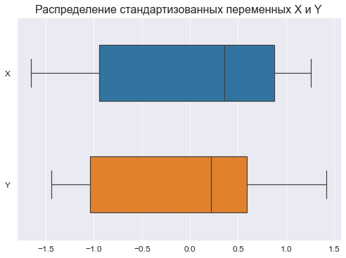
Графический анализ позволяет сделать следующие выводы:
-
Отсутствие выбросов на коробчатых диаграммах свидетельствует об однородности распределения переменных.
-
Смещение медианы вправо на коробчатых диаграммах свидетельствует о левосторонней асимметрии распределения.
ДЕСКРИПТИВНАЯ (ОПИСАТЕЛЬНАЯ СТАТИСТИКА)
Собственно говоря, данный этап требуется проводить далеко не всегда, однако с помощью статистических характеристик выборки мы тоже можем сделать полезные выводы.
Описательная статистика исходных данных средствами библиотеки Pandas — самый простой вариант:
dataset_df.describe()
Описательная статистика исходных данных средствами библиотеки statsmodels — более развернутый вариант, с большим количеством показателей:
from statsmodels.stats.descriptivestats import Description
result = Description(
    dataset_df,
    stats=["nobs", "missing", "mean", "std_err", "ci", "ci", "std", "iqr", "mad", "coef_var", "range", "max", "min", "skew", "kurtosis", "mode",
           "median", "percentiles", "distinct", "top", "freq"],
    alpha=a_level,
    use_t=True)
display(result.summary())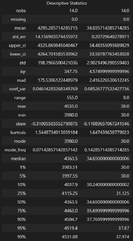
Описательная статистика исходных данных с помощью пользовательской функции descriptive_characteristics:
# Пользовательская функция
descriptive_characteristics(X)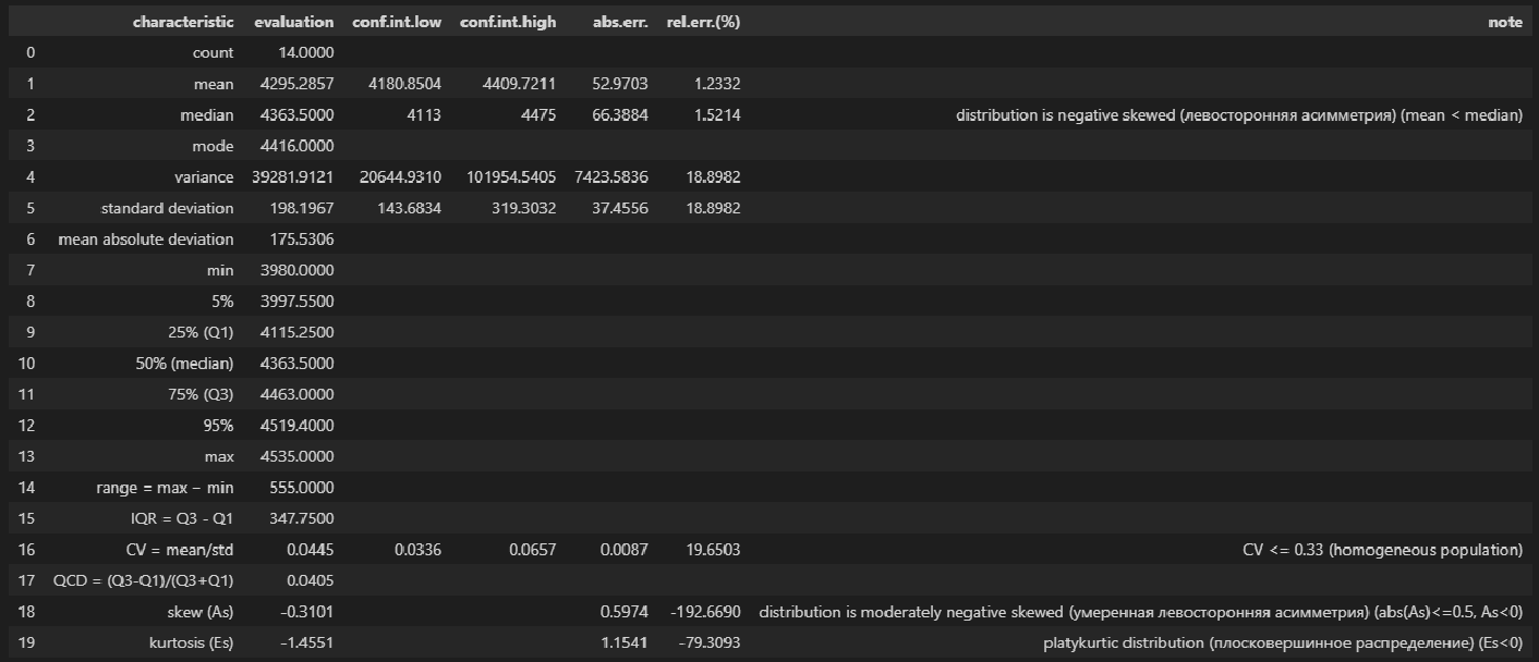
Выводы:
-
Сравнение показателей среднего арифметического (mean) и медианы (median) свидетельствует о левосторонней асимметрии (т.к.mean < median).
-
Значение коэффициента вариации CV = 0.0445 и доверительный интервал для него 0.0336 ≤ CV ≤ 0.0657 свидетельствует об однородности исходных данных (т.к. CV ≤ 0.33).
-
Значение показателя асимметрии skew (As) = -0.3101 свидетельствует об умеренной левосторонней асимметрии распределении (т.к. |As| ≤ 0.5, As < 0).
-
Значение показателя эксцесса kurtosis (Es) = -1.4551 свидетельствует о плосковершинном распределении (platykurtic distribution) (т.к. Es < 0).
# Пользовательская функция
descriptive_characteristics(Y)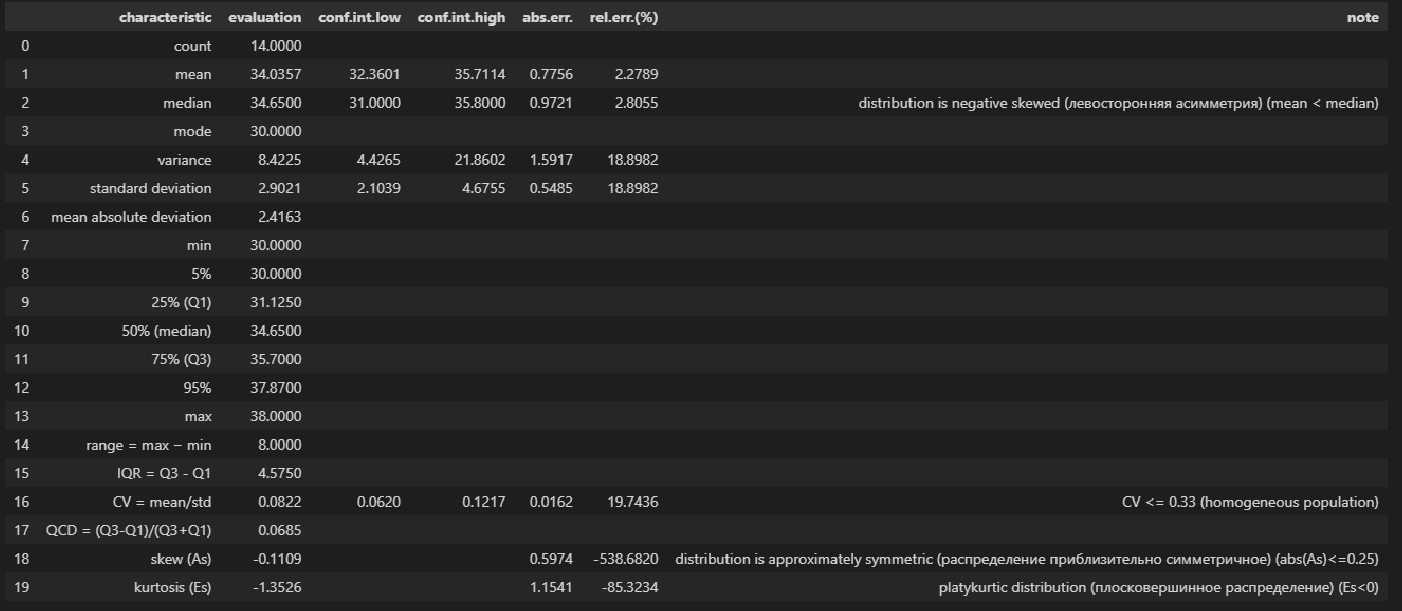
Выводы:
-
Сравнение показателей среднего арифметического (mean) и медианы (median) свидетельствует о левосторонней асимметрии (т.к.mean < median).
-
Значение коэффициента вариации CV = 0.0822 и доверительный интервал для него 0.06202 ≤ CV ≤ 0.1217 свидетельствует об однородности исходных данных (т.к. CV ≤ 0.33).
-
Значение показателя асимметрии skew (As) = -0.1109 свидетельствует о приблизительно симметричном распределении (т.к. |As| ≤ 0.25).
-
Значение показателя эксцесса kurtosis (Es) = -1.3526 свидетельствует о плосковершинном распределении (platykurtic distribution) (т.к. Es < 0).
ПРОВЕРКА НОРМАЛЬНОСТИ РАСПРЕДЕЛЕНИЯ
Для проверки нормальности распределения использована пользовательская функция norm_distr_check, которая объединяет в себе набор стандартных статистических тестов проверки нормальности. Все тесты относятся к стандартному инструментарию Pyton (библиотека scipy, модуль stats), за исключением теста Эппса-Палли (Epps-Pulley test); о том, как реализовать этот тест средствами Pyton я писал в своей статье https://habr.com/ru/post/685582/.
Примечание: для использования функции norm_distr_check в каталог с ipynb-файлом необходимо поместить папку table c файлом Tep_table.csv, который содержит табличные значения статистики критерия Эппса-Палли.
# пользовательская функция
norm_distr_check(X)
# Пользовательская функция
norm_distr_check (Y)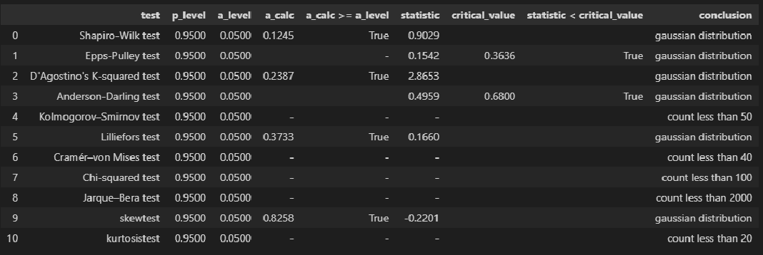
Вывод: большинство статистических тестов позволяют принять гипотезу о нормальности распределения переменных X и Y.
ПРОВЕРКА АНОМАЛЬНЫХ ЗНАЧЕНИЙ (ВЫБРОСОВ)
Статистическую проверку аномальных значений (выбросов) не стоит путать с проверкой выбросов, которая проводится на этапе первичной обработки результатов наблюдений. Последняя проводится с целью отсеять явные ошибочные данные (например, в результате неправильно поставленной запятой величина показателя может увеличиться/уменьшиться на порядок); здесь же мы говорим о статистической проверке данных, которые уже прошли этап первичной обработки.
Имеется довольно много критериев для проверки аномальных значений (подробнее см.[1]); вообще данная процедура довольно неоднозначная:
-
критерии зависят от вида распределения;
-
мало данных о сравнительной мощности этих критериев;
-
даже в случае принятии гипотезы о нормальном распределении в выборке могут быть обнаружены аномальные значения и пр.
Кроме существует дилемма: если какие-то значения в выборке признаны выбросами — стоит или не стоит исследователю исключать их? Ведь каждое значение несет в себе информацию, причем иногда весьма ценную, а сильно отклоняющиеся от основного массива данные (которые не являются выбросами в смысле первичной обработки, но являются статистическим значимыми аномальными значениями) могут кардинально изменить статистический вывод.
В общем, о задаче выявления аномальных значений (выбросов) можно написать отдельно, а пока, в данном разборе, ограничимся проверкой аномальных значений по критерию наибольшего максимального отклонения (см.[1, с.547]) с помощью пользовательской функции detecting_outliers_mad_test. Данные функция возвращает DataFrame, которые включает список аномальных значений со следующими признаками:
-
value — проверяемое значение из выборки;
-
mad_calc и mad_table — расчетное и табличное значение статистики критерия;
-
outlier_conclusion — вывод (выброс или нет).
Обращаю внимание, что критерий наибольшего максимального отклонения можно использовать только для нормально распределенных данных.
# пользовательская функция
print("Проверка наличия выбросов переменной X:n")
result = detecting_outliers_mad_test(X)
mask = (result['outlier_conclusion'] == 'outlier')
display(result[mask])
# пользовательская функция
print("Проверка наличия выбросов переменной Y:n")
result = detecting_outliers_mad_test(Y)
mask = (result['outlier_conclusion'] == 'outlier')
display(result[mask])
Вывод: в случае обеих переменных X и Y список пуст, следовательно, аномальных значений (выбросов) не выявлено.
КОРРЕЛЯЦИОННЫЙ АНАЛИЗ
Корреляционный анализ — это разведка перед построением регрессионной модели.
Выполним расчет коэффициента линейной корреляции Пирсона, проверку его значимости и построение доверительных интервалов с помощью пользовательской функции corr_coef_check (про эту функцию более подробно написано в моей статье https://habr.com/ru/post/683442/):
# пользовательская функция
display(corr_coef_check(X, Y, scale='Evans'))
Выводы:
-
Значение коэффициента корреляции coef_value = 0.8900 свидетельствует о весьма сильной корреляционной связи (по шкале Эванса).
-
Коэффициент корреляции значим по критерию Стьюдента: t_calc ≥ t_table, a_calc ≤ a_level.
-
Доверительный интервал для коэффициента корреляции: 0.6621 ≤ coef_value ≤ 0.9625.
РЕГРЕССИОННЫЙ АНАЛИЗ
Предварительная визуализация
python позволяет выполнить предварительную визуализацию, например, с помощью функции jointplot библиотеки seaborn:
fig = plt.figure(figsize=(297/INCH, 210/INCH))
axes = sns.jointplot(
    x=X, y=Y,
    kind='reg',
    ci=95)
plt.show()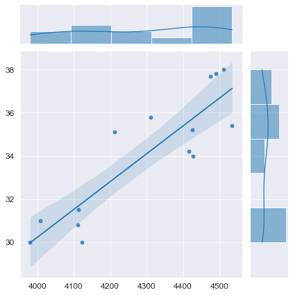
Построение модели
Выполним оценку параметров и анализ простой линейной регрессии (simple linear regression), используя библиотеку statsmodels (https://www.statsmodels.org/) и входящий в нее модуль линейной регрессии Linear Regression (https://www.statsmodels.org/stable/regression.html).
Данный модуль включает в себя классы, реализующие различные методы оценки параметров моделей линейной регрессии, в том числе:
-
класс OLS (https://www.statsmodels.org/stable/generated/statsmodels.regression.linear_model.OLS.html#statsmodels.regression.linear_model.OLS) — Ordinary Least Squares (обычный метод наименьших квадратов).
-
класс WLS (https://www.statsmodels.org/stable/generated/statsmodels.regression.linear_model.WLS.html#statsmodels.regression.linear_model.WLS) — Weighted Least Squares (метод взвешенных наименьших квадратов) (https://en.wikipedia.org/wiki/Weighted_least_squares), применяется, если имеет место гетероскедастичность данных (https://ru.wikipedia.org/wiki/Гетероскедастичность).
-
класс GLS (https://www.statsmodels.org/stable/generated/statsmodels.regression.linear_model.GLS.html#statsmodels.regression.linear_model.GLS) — Generalized Least Squares (обобщенный метод наименьших квадратов) (https://en.wikipedia.org/wiki/Generalized_least_squares), применяется, если существует определенная степень корреляции между остатками в модели регрессии.
-
класс GLSAR (https://www.statsmodels.org/stable/generated/statsmodels.regression.linear_model.GLSAR.html#statsmodels.regression.linear_model.GLSAR) — Generalized Least Squares with AR covariance structure (обобщенный метод наименьших квадратов, ковариационная структура с автокорреляцией — экспериментальный метод)
-
класс RecurciveLS (https://www.statsmodels.org/stable/examples/notebooks/generated/recursive_ls.html) — Recursive least squares (рекурсивный метод наименьших квадратов) (https://en.wikipedia.org/wiki/Recursive_least_squares_filter)
-
классы RollingOLS (https://www.statsmodels.org/stable/generated/statsmodels.regression.rolling.RollingOLS.html#statsmodels.regression.rolling.RollingOLS) и RollingWLS (https://www.statsmodels.org/stable/generated/statsmodels.regression.rolling.RollingWLS.html#statsmodels.regression.rolling.RollingWLS) — скользящая регрессия (https://www.statsmodels.org/stable/examples/notebooks/generated/rolling_ls.html, https://help.fsight.ru/ru/mergedProjects/lib/01_regression_models/rolling_regression.htm)
и т.д.
Так как исходные данные подчиняются нормальному закону распределения и аномальные значения (выбросы) отсутствуют, воспользуемся для оценки параметров обычным методом наименьших квадратов (класс OLS):
model_linear_ols = smf.ols(formula='Y ~ X', data=dataset_df)
result_linear_ols = model_linear_ols.fit()
print(result_linear_ols.summary())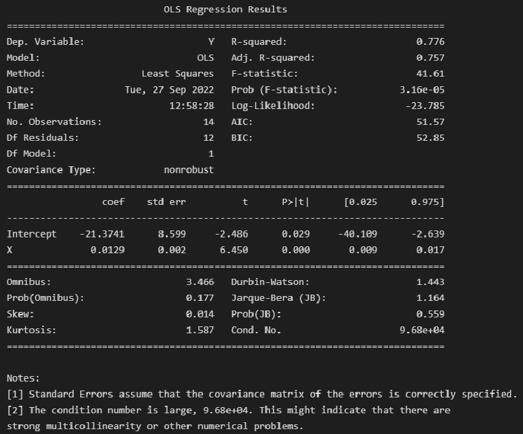
Альтернативная форма выдачи результатов:
print(result_linear_ols.summary2())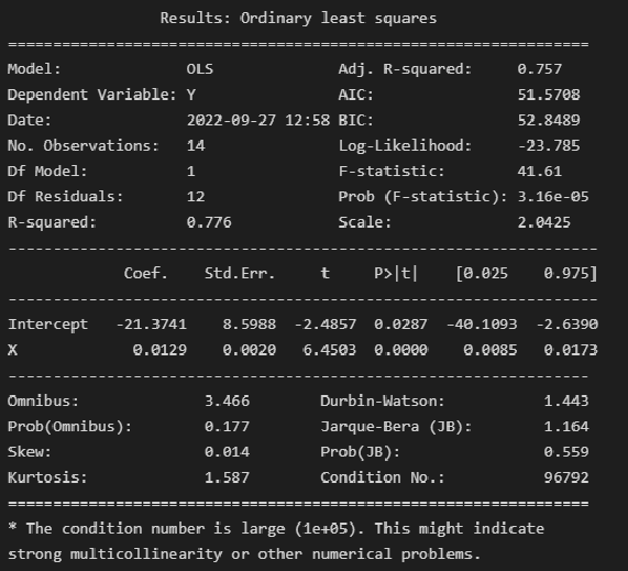
Результаты построения модели мы получаем как класс statsmodels.regression.linear_model.RegressionResults (https://www.statsmodels.org/stable/generated/statsmodels.regression.linear_model.RegressionResults.html#statsmodels.regression.linear_model.RegressionResults).
Экспресс-выводы, которые мы можем сразу сделать из результатов построения модели:
-
Коэффициенты регрессии модели Y = b0 + b1∙X:
-
Intercept = b0 = -21.3741
-
b1 = 0.0129
-
-
Коэффициент детерминации R-squared = 0.776, его скорректированная оценка Adj. R-squared = 0.757 — это означает, что регрессионная модуль объясняет 75.75% вариации переменной Y.
-
Проверка значимости коэффициента детерминации:
-
расчетное значение статистики критерия Фишера: F-statistic = 41.61
-
расчетный уровень значимости Prob (F-statistic) = 3.16e-05
-
так как значение Prob (F-statistic) < 0.05, то нулевая гипотеза R-squared = 0 НЕ ПРИНИМАЕТСЯ, т.е. коэффициент детерминации ЗНАЧИМ
-
-
Проверка значимости коэффициентов регрессии:
-
расчетный уровень значимости P>|t| не превышает 0.05 — это означает, что оба коэффициента регрессии значимы
-
об этом же свидетельствует то, что доверительный интервал для обоих коэффициентов регрессии ([0.025; 0.975]) не включает в себя точку 0
Также в таблице результатов содержится прочая информация по коэффициентам регрессии: стандартная ошибка Std.Err. расчетное значение статистики критерия Стьюдента t для проверки гипотезы о значимости.
-
-
Анализ остатков модели:
-
Тест Omnibus — про этот тест подробно написано в https://en.wikipedia.org/wiki/Omnibus_test, https://medium.com/swlh/interpreting-linear-regression-through-statsmodels-summary-4796d359035a, http://work.thaslwanter.at/Stats/html/statsModels.html.
Расчетное значение статистики критерия Omnibus = 3.466 — по сути расчетное значение F-критерия (см. https://en.wikipedia.org/wiki/Omnibus_test).
Prob(Omnibus) = 0.177 — показывает вероятность нормального распределения остатков (значение 1 указывает на совершенно нормальное распределение).
Учитывая, что в дальнейшем мы проверим нормальность распределения остатков по совокупности различных тестов, в том числе с достаточно высокой мощностью, и все тесты позволят принять гипотезу о нормальном распределении — в данном случае к тесту Omnibus возникают вопросы. С этим тестом нужно разбираться отдельно.
-
Skew = 0.014 и Kurtosis = 1.587 — показатели асимметрии и эксцесса остатков свидетельствуют, что распределение остатков практически симметричное, островершинное.
-
проверка нормальности распределения остатков по критерию Харке-Бера: расчетное значение статистики критерия Jarque-Bera (JB) = 1.164 и расчетный уровень значимости Prob(JB) = 0.559. К данным результатам также возникают вопросы, особенно, если учесть, что критерий Харке-Бера является асимптотическим, расчетное значение имеет распределение хи-квадрат, поэтому данный критерий рекомендуют применять только для больших выборок (см. https://en.wikipedia.org/wiki/Jarque–Bera_test). Проверку нормальности распределения остатков модели лучше проводить с использованием набора стандартных статистических тестов python (см. далее).
-
-
Проверка автокорреляции по критерию Дарбина-Уотсона: Durbin-Watson = 1.443.
Мы не будем здесь разбирать данный критерий, так как явление автокорреляции больше характерно для данных, выражаемых в виде временных рядов. Однако, для грубой оценки считается, что при расчетном значении статистики криетрия Дарбина=Уотсона а интервале [1; 2] автокорреляция отсутствует (см.https://en.wikipedia.org/wiki/Durbin–Watson_statistic).
Более подробно про критерий Дарбина-Уотсона — см. [1, с.659].
Прочая информация, которую можно извлечь из результатов построения модели:
-
Covariance Type — тип ковариации, подробнее см. https://habr.com/ru/post/681218/, https://towardsdatascience.com/simple-explanation-of-statsmodel-linear-regression-model-summary-35961919868b#:~:text=Covariance type is typically nonrobust,with respect to each other.
-
Scale — масштабный коэффициент для ковариационной матрицы (https://www.statsmodels.org/stable/generated/statsmodels.regression.linear_model.RegressionResults.scale.html#statsmodels.regression.linear_model.RegressionResults.scale), равен величине Mean squared error (MSE) (cреднеквадратической ошибке), об подробнее см. далее, в разделе про ошибки аппроксимации моделей.
-
Показатели сравнения качества различных моделей:
-
Log-Likelihood — логарифмическая функция правдоподобия, подробнее см. https://en.wikipedia.org/wiki/Likelihood_function#Log-likelihood, https://habr.com/ru/post/433804/
-
AIC — информационный критерий Акаике (Akaike information criterion), подробнее см. https://en.wikipedia.org/wiki/Akaike_information_criterion
-
BIC — информационный критерий Байеса (Bayesian information criterion), подробнее см. https://en.wikipedia.org/wiki/Bayesian_information_criterion
В данной статье мы эти показатели рассматривать не будем, так как задача выбора одной модели из нескольких перед нами не стоит.
-
-
Число обусловленности Cond. No = 96792 используется для проверки мультиколлинеарности (считается, что мультиколлинеарность есть, если значение Cond. No > 30) (см. http://work.thaslwanter.at/Stats/html/statsModels.html). В нашем случае парной регрессионной модели о мультиколлинеарности речь не идет.
Далее будем извлекать данные из стандартного набора выдачи результатов и анализировать их более подробно. Последующие этапы вовсе не обязательно проводить в полном объеме при решении задач, но здесь мы рассмотрим их подробно.
Параметры и уравнение регрессионной модели
Извлечем параметры полученной модели — как свойство params модели:
print('Параметры модели: n', result_linear_ols.params, type(result_linear_ols.params))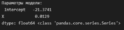
Имея параметры модели, можем формализовать уравнение модели Y = b0 + b1*X:
b0 = result_linear_ols.params['Intercept']
b1 = result_linear_ols.params['X']
Y_calc = lambda x: b0 + b1*x
График регрессионной модели
Для построения графиков регрессионных моделей можно воспользоваться стандартными возможностями библиотек statsmodels, seaborn, либо создать пользовательскую функцию — на усмотрение исследователя:
1. Построение графиков регрессионных моделей с использованием библиотеки statsmodels
С помощью функции statsmodels.graphics.plot_fit (https://www.statsmodels.org/stable/generated/statsmodels.graphics.regressionplots.plot_fit.html#statsmodels.graphics.regressionplots.plot_fit) — отображается график Y and Fitted vs.X (фактические и расчетные значения Y с доверительным интервалом для каждого значения Y):
fig, ax = plt.subplots(figsize=(297/INCH, 210/INCH))
fig = sm.graphics.plot_fit(
    result_linear_ols, 'X',
    vlines=True,    # это параметр отвечает за отображение доверительных интервалов для Y
    ax=ax)
ax.set_ylabel(Variable_Name_Y)
ax.set_xlabel(Variable_Name_X)
ax.set_title(Task_Project)
plt.show()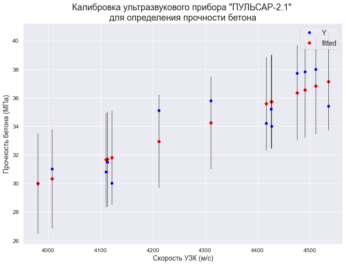
С помощью функции statsmodels.graphics.plot_regress_exog (https://www.statsmodels.org/stable/generated/statsmodels.graphics.regressionplots.plot_regress_exog.html#statsmodels.graphics.regressionplots.plot_regress_exog) — отображается область 2х2, которая содержит:
-
предыдущий график Y and Fitted vs.X;
-
график остатков Residuals versus X;
-
график Partial regression plot — график частичной регрессии, пытается показать эффект добавления другой переменной в модель, которая уже имеет одну или несколько независимых переменных (более подробно см. https://en.wikipedia.org/wiki/Partial_regression_plot);
-
график CCPR Plot (Component-Component plus Residual Plot) — еще один способ оценить влияние одной независимой переменной на переменную отклика, принимая во внимание влияние других независимых переменных (более подробно — см. https://towardsdatascience.com/calculating-price-elasticity-of-demand-statistical-modeling-with-python-6adb2fa7824d, https://www.kirenz.com/post/2021-11-14-linear-regression-diagnostics-in-python/linear-regression-diagnostics-in-python/).
fig = plt.figure(figsize=(297/INCH, 210/INCH))
sm.graphics.plot_regress_exog(result_linear_ols, 'X', fig=fig)
plt.show()
2. Построение графиков регрессионных моделей с использованием библиотеки seaborn
Воспользуемся модулем regplot библиотеки seaborn (https://seaborn.pydata.org/generated/seaborn.regplot.html). Данный модуль позволяет визуализировать различные виды регрессии:
-
линейную
-
полиномиальную
-
логистическую
-
взвешенную локальную регрессию (LOWESS — Locally Weighted Scatterplot Smoothing) (см. http://www.machinelearning.ru/wiki/index.php?title=Алгоритм_LOWESS, https://www.statsmodels.org/stable/generated/statsmodels.nonparametric.smoothers_lowess.lowess.html)
Более подробно про модуль regplot можно прочитать в статье: https://pyprog.pro/sns/sns_8_regression_models.html.
Есть более совершенный модуль lmplot (https://seaborn.pydata.org/generated/seaborn.lmplot.html), который объединяет в себе regplot и FacetGrid, но мы его здесь рассматривать не будем.
# создание рисунка (Figure) и области рисования (Axes)
fig = plt.figure(figsize=(297/INCH, 420/INCH/1.5))
ax1 = plt.subplot(2,1,1)
ax2 = plt.subplot(2,1,2)
# заголовок рисунка (Figure)
title_figure = Task_Project
fig.suptitle(title_figure, fontsize = 18)
# заголовок области рисования (Axes)
title_axes_1 = 'Линейная регрессионная модель'
ax1.set_title(title_axes_1, fontsize = 16)
# график регрессионной модели
order_mod = 1    # порядок модели
#label_legend_regr_model = 'фактические данные'
sns.regplot(
    #data=dataset_df,
    x=X, y=Y,
    #x_estimator=np.mean,
    order=order_mod,
    logistic=False,
    lowess=False,
    robust=False,
    logx=False,
    ci=95,
    scatter_kws={'s': 30, 'color': 'red'},
    line_kws={'color': 'blue'},
    #label=label_legend_regr_model,
    ax=ax1)
ax1.set_ylabel(Variable_Name_Y)
ax1.legend()
# график остатков
title_axes_2 = 'График остатков'
ax2.set_title(title_axes_2, fontsize = 16)
sns.residplot(
    #data=dataset_df,
    x=X, y=Y,
    order=order_mod,
    lowess=False,
    robust=False,
    scatter_kws={'s': 30, 'color': 'darkorange'},
    ax=ax2)
ax2.set_xlabel(Variable_Name_X)

plt.show()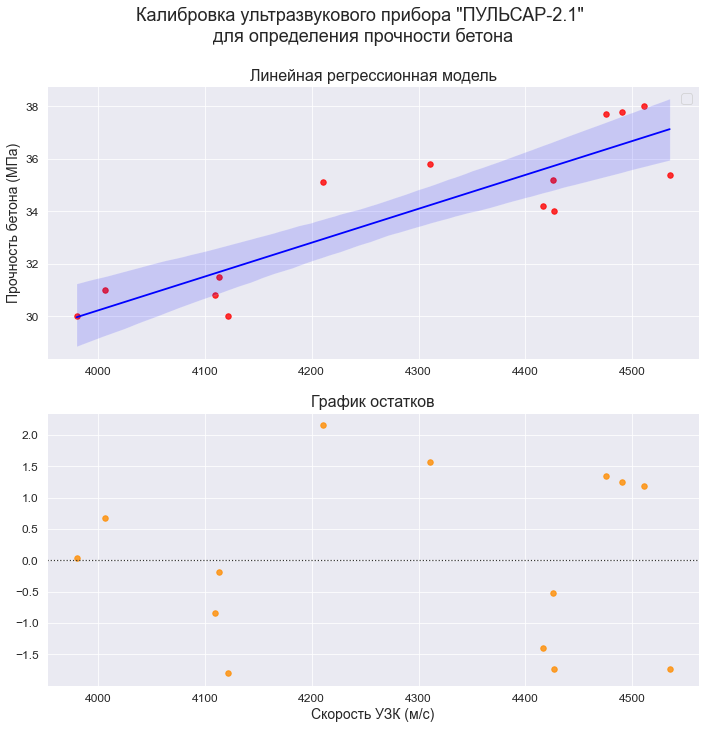
3. Построение графиков регрессионных моделей с помощью пользовательской функции
# Пользовательская функция
graph_regression_plot_sns(
    X, Y,
    regression_model=Y_calc,
    Xmin=Xmin_graph, Xmax=Xmax_graph,
    Ymin=Ymin_graph, Ymax=Ymax_graph,
    title_figure=Task_Project,
    x_label=Variable_Name_X,
    y_label=Variable_Name_Y,
    label_legend_regr_model=f'линейная регрессия Y = {b0:.3f} + {b1:.4f}*X',
    s=80,
    file_name='graph/regression_plot_lin.png')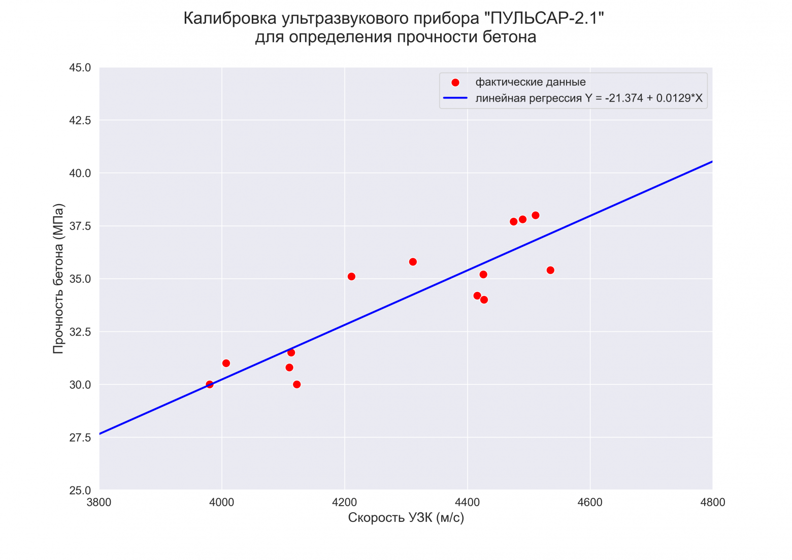
Статистический анализ регрессионной модели
1. Расчет ошибки аппроксимации (Error Metrics)
Ошибки аппроксимации (Error Metrics) позволяют получить общее представление о качестве модели, а также позволяют сравнивать между собой различные модели.
Создадим пользовательскую функцию, которая рассчитывает основные ошибки аппроксимации для заданной модели:
-
Mean squared error (MSE) или Mean squared deviation (MSD) — среднеквадратическая ошибка (https://en.wikipedia.org/wiki/Mean_squared_error):

-
Root mean square error (RMSE) или Root mean square deviation (RMSD) — квадратный корень из MSE (https://en.wikipedia.org/wiki/Root-mean-square_deviation):
![]()
-
Mean absolute error (MAE) — средняя абсолютная ошибка (https://en.wikipedia.org/wiki/Mean_absolute_error):

-
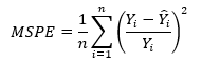
Mean squared prediction error (MSPE) — среднеквадратическая ошибка прогноза (среднеквадратическая ошибка в процентах) (https://en.wikipedia.org/wiki/Mean_squared_prediction_error):
-
Mean absolute percentage error (MAPE) — средняя абсолютная ошибка в процентах (https://en.wikipedia.org/wiki/Mean_absolute_percentage_error):

Про выбор метрики см. также https://machinelearningmastery.ru/how-to-select-the-right-evaluation-metric-for-machine-learning-models-part-2-regression-metrics-d4a1a9ba3d74/.
# Пользовательская функция
def regression_error_metrics(model, model_name=''):
    model_fit = model.fit()
    Ycalc = model_fit.predict()
    n_fit = model_fit.nobs
    Y = model.endog

    MSE = (1/n_fit) * np.sum((Y-Ycalc)**2)
    RMSE = sqrt(MSE)
    MAE = (1/n_fit) * np.sum(abs(Y-Ycalc))
    MSPE = (1/n_fit) *  np.sum(((Y-Ycalc)/Y)**2)
    MAPE = (1/n_fit) *  np.sum(abs((Y-Ycalc)/Y))

    model_error_metrics = {
        'MSE': MSE,
        'RMSE': RMSE,
        'MAE': MAE,
        'MSPE': MSPE,
        'MAPE': MAPE}

    result = pd.DataFrame({
        'MSE': MSE,
        'RMSE': RMSE,
        'MAE': MAE,
        'MSPE': "{:.3%}".format(MSPE),
        'MAPE': "{:.3%}".format(MAPE)},
        index=[model_name])

    return model_error_metrics, result

(model_error_metrics, result) = regression_error_metrics(model_linear_ols, model_name='linear_ols')
display(result)
В литературе по прикладной статистике нет единого мнения о допустимом размере относительных ошибок аппроксимации: в одних источниках допустимой считается ошибка 5-7%, в других она может быть увеличена до 8-10%, и даже до 15%.
Вывод: модель хорошо аппроксимирует фактические данные (относительная ошибка аппроксимации MAPE = 3.405% < 10%).
2. Дисперсионный анализ регрессионной модели (ДАРМ)
ДАРМ не входит в стандартную форму выдачи результатов Regression Results, однако я решил написать здесь о нем по двум причинам:
-
Именно анализ дисперсии регрессионной модели, разложение этой дисперсии на составляющие дает фундаментальное представление о сути регрессии, а термины, используемые при ДАРМ, применяются на последующих этапах анализа.
-
С терминами ДАРМ в литературе по прикладной статистике имеется некоторая путаница, в разных источниках они могут именоваться по-разному (см., например, [8, с.52]), поэтому, чтобы двигаться дальше, необходимо определиться с понятиями.
При ДАРМ общую вариацию результативного признака (Y) принято разделять на две составляющие — вариация, обусловленная регрессией и вариация, обусловленная отклонениями от регрессии (остаток), при этом в разных источниках эти термины могут именоваться и обозначаться по-разному, например:
-
Вариация, обусловленная регрессией — может называться Explained sum of squares (ESS), Sum of Squared Regression (SSR) (https://en.wikipedia.org/wiki/Explained_sum_of_squares, https://towardsdatascience.com/anova-for-regression-fdb49cf5d684), Sum of squared deviations (SSD).
-
Вариация, обусловленная отклонениями от регрессии (остаток) — может называться Residual sum of squares (RSS), Sum of squared residuals (SSR), Squared estimate of errors, Sum of Squared Error (SSE) (https://en.wikipedia.org/wiki/Residual_sum_of_squares, https://towardsdatascience.com/anova-for-regression-fdb49cf5d684); в отчественной практике также применяется термин остаточная дисперсия.
-
Общая (полная) вариация — может называться Total sum of squares (TSS), Sum of Squared Total (SST) (https://en.wikipedia.org/wiki/Partition_of_sums_of_squares, https://towardsdatascience.com/anova-for-regression-fdb49cf5d684).
Как видим, путаница знатная:
-
в разных источниках под SSR могут подразумеваться различные показатели;
-
легко перепутать показатели ESS и SSE;
-
в библиотеке statsmodel также есть смешение терминов: для показателя Explained sum of squares используется свойство ess, а для показателя Sum of squared (whitened) residuals — свойство ssr.
Мы будем пользоваться системой обозначений, принятой в большинстве источников — SSR (Sum of Squared Regression), SSE (Sum of Squared Error), SST (Sum of Squared Total). Стандартная таблица ДАРМ в этом случае имеет вид:

Примечания:
-
Здесь приведена таблица ДАРМ для множественной линейной регрессионной модели (МЛРМ), в нашем случае при ПЛРМ мы имеем частный случай p=1.
-
Показатели Fcalc-ad и Fcalc-det — расчетные значения статистики критерия Фишера при проверке адекватности модели и значимости коэффициента детерминации (об этом — см.далее).
Более подробно про дисперсионный анализ регрессионной модели — см.[4, глава 3].
Класс statsmodels.regression.linear_model.RegressionResults позволяет нам получить данные для ANOVA (см. https://www.statsmodels.org/stable/generated/statsmodels.regression.linear_model.RegressionResults.html#statsmodels.regression.linear_model.RegressionResults) как свойства класса:
-
Сумма квадратов, обусловленная регрессией / SSR (Sum of Squared Regression) — свойство ess.
-
Сумма квадратов, обусловленная отклонением от регрессии / SSE (Sum of Squared Error) — свойство ssr.
-
Общая (полная) сумма квадратов / SST (Sum of Squared Total) — свойство centered_tss.
-
Кол-во наблюдений / Number of observations — свойство nobs.
-
Число степеней свободы модели / Model degrees of freedom — равно числу переменных модели (за исключением константы, если она присутствует — свойство df_model.
-
Среднеквадратичная ошибка модели / Mean squared error the model — сумма квадратов, объясненная регрессией, деленная на число степеней свободы регрессии — свойство mse_model.
-
Среднеквадратичная ошибка остатков / Mean squared error of the residuals — сумма квадратов остатков, деленная на остаточные степени свободы — свойство mse_resid.
-
Общая среднеквадратичная ошибка / Total mean squared error — общая сумма квадратов, деленная на количество наблюдений — свойство mse_total.
Также имеется модуль statsmodels.stats.anova.anova_lm, который позволяет получить результаты ДАРМ (нескольких типов — 1, 2, 3):
# тип 1
print('The type of Anova test: 1')
display(sm.stats.anova_lm(result_linear_ols, typ=1))

# тип 2
print('The type of Anova test: 2')
display(sm.stats.anova_lm(result_linear_ols, typ=2))

# тип 3
print('The type of Anova test: 3')
display(sm.stats.anova_lm(result_linear_ols, typ=3))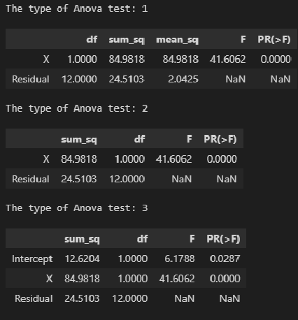
На мой взгляд, форма таблица результатов statsmodels.stats.anova.anova_lm не вполне удобна, поэтому сформируем ее самостоятельно, для чего создадим пользовательскую функцию ANOVA_table_regression_model:
# Пользовательская функция
def ANOVA_table_regression_model(model_fit):
    n = int(model_fit.nobs)
    p = int(model_fit.df_model)
    SSR = model_fit.ess
    SSE = model_fit.ssr
    SST = model_fit.centered_tss

    result = pd.DataFrame({
        'sources_of_variation': ('regression (SSR)', 'deviation from regression (SSE)', 'total (SST)'),
        'sum_of_squares': (SSR, SSE, SST),
        'degrees_of_freedom': (p, n-p-1, n-1)})
    result['squared_error'] = result['sum_of_squares'] / result['degrees_of_freedom']
    R2 = 1 - result.loc[1, 'sum_of_squares'] / result.loc[2, 'sum_of_squares']
    F_calc_adequacy = result.loc[2, 'squared_error'] / result.loc[1, 'squared_error']
    F_calc_determ_check = result.loc[0, 'squared_error'] / result.loc[1, 'squared_error']
    result['F-ratio'] = (F_calc_determ_check, F_calc_adequacy, '')

    return result

result = ANOVA_table_regression_model(result_linear_ols)
display(result)
print(f"R2 = 1 - SSE/SST = {1 - result.loc[1, 'sum_of_squares'] / result.loc[2, 'sum_of_squares']}")
print(f"F_calc_adequacy = MST / MSE = {result.loc[2, 'squared_error'] / result.loc[1, 'squared_error']}")
print(f"F_calc_determ_check = MSR / MSE = {result.loc[0, 'squared_error'] / result.loc[1, 'squared_error']}")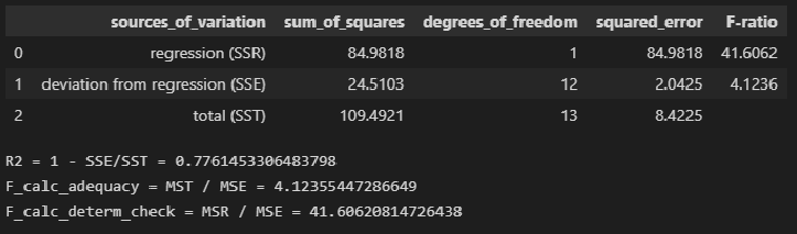
ДАРМ позволяет визуализировать вариацию:
fig, axes = plt.subplots(figsize=(210/INCH, 297/INCH/1.5))
axes.pie(
    (result.loc[0, 'sum_of_squares'], result.loc[1, 'sum_of_squares']),
    labels=(result.loc[0, 'sources_of_variation'], result.loc[1, 'sources_of_variation']),
    autopct='%.1f%%',
    startangle=60)
plt.show()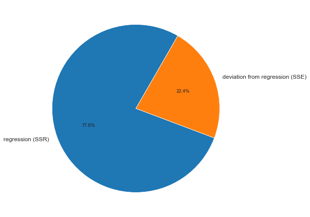
На основании данных ДАРМ мы рассчитали ряд показателей (R2, Fcalc-ad и Fcalc-det), которые будут использоваться в дальнейшем.
3. Анализ остатков (проверка нормальности распределения остатков и гипотезы о равенстве нулю среднего значения остатков)
Проверка нормальности распределения остатков — один их важнейших этапов анализа регрессионной модели. Требование нормальности распределения остатков не требуется для отыскания параметров модели, но необходимо в дальнейшем для проверки статистических гипотез с использованием критериев Фишера и Стьюдента (проверка адекватности модели, значимости коэффициента детерминации, значимости коэффициентов регрессии) и построения доверительных интервалов [5, с.122].
Остатки регрессионной модели:
print('Остатки регрессионной модели:n', result_linear_ols.resid, type(result_linear_ols.resid))
res_Y = np.array(result_linear_ols.resid)
statsmodels может выдавать различные преобразованные виды остатков (см. https://www.statsmodels.org/stable/generated/statsmodels.regression.linear_model.RegressionResults.resid_pearson.html, https://www.statsmodels.org/stable/generated/statsmodels.regression.linear_model.RegressionResults.wresid.html).
График остатков:
# Пользовательская функция
graph_scatterplot_sns(
    X, res_Y,
    Xmin=Xmin_graph, Xmax=Xmax_graph,
    Ymin=-3.0, Ymax=3.0,
    color='red',
    #title_figure=Task_Project,
    title_axes='Остатки линейной регрессионной модели', title_axes_fontsize=18,
    x_label=Variable_Name_X,
    y_label='ΔY = Y - Ycalc',
    s=75,
    file_name='graph/residuals_plot_sns.png')
Проверка нормальности распределения остатков:
# Пользовательская функция
graph_hist_boxplot_probplot_sns(
    data=res_Y,
    data_min=-2.5, data_max=2.5,
    graph_inclusion='bp',
    data_label='ΔY = Y - Ycalc',
    #title_figure=Task_Project,
    title_axes='Остатки линейной регрессионной модели', title_axes_fontsize=16,
file_name='graph/residuals_hist_boxplot_probplot_sns.png') 
norm_distr_check(res_Y)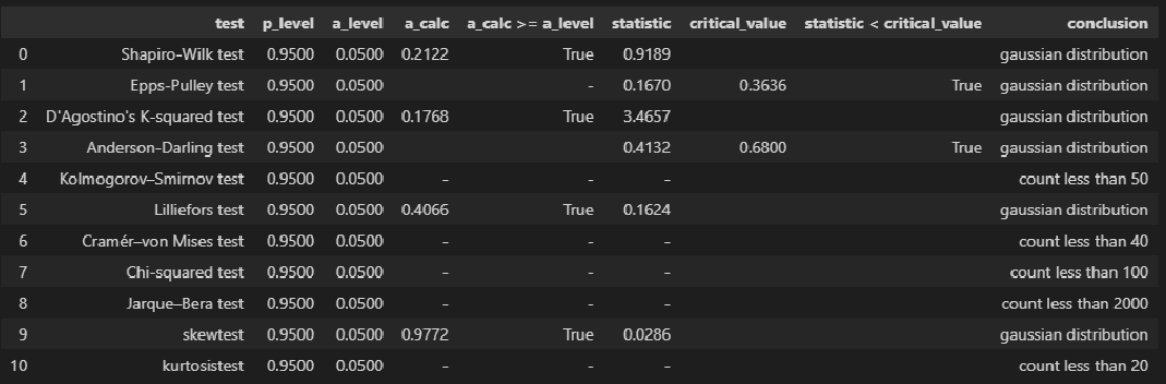
Вывод: большинство статистических тестов позволяют принять гипотезу о нормальности распределения остатков.
Проверка гипотезы о равенстве нулю среднего значения остатков — так как остатки имеют нормальное распределение, воспользуемся критерием Стьюдента (функция scipy.stats.ttest_1samp, https://docs.scipy.org/doc/scipy/reference/generated/scipy.stats.ttest_ind.html):
sps.ttest_1samp(res_Y, popmean=0)![]()
Вывод: так как расчетный уровень значимости превышает заданный (0.05), то нулевая гипотеза о равенстве нулю остатков ПРИНИМАЕТСЯ.
4. Проверка адекватности модели
Суть проверки адекватности регрессионной модели заключается в сравнении полной дисперсии MST и остаточной дисперсии MSE — проверяется гипотеза о равенстве этих дисперсий по критерию Фишера. Если дисперсии различаются значимо, то модель считается адекватной. Более подробно про проверку адекватности регрессионной — см.[1, с.658], [2, с.49], [4, с.154].
Для проверки адекватности регрессионной модели создадим пользовательскую функцию regression_model_adequacy_check:
def regression_model_adequacy_check(
    model_fit,
    p_level: float=0.95,
    model_name=''):

    n = int(model_fit.nobs)
    p = int(model_fit.df_model)    # Число степеней свободы регрессии, равно числу переменных модели (за исключением константы, если она присутствует)

    SST = model_fit.centered_tss    # SST (Sum of Squared Total)
    dfT = n-1
    MST = SST / dfT

    SSE = model_fit.ssr    # SSE (Sum of Squared Error)
    dfE = n - p - 1
    MSE = SSE / dfE

    F_calc = MST / MSE
    F_table = sci.stats.f.ppf(p_level, dfT, dfE, loc=0, scale=1)
    a_calc = 1 - sci.stats.f.cdf(F_calc, dfT, dfE, loc=0, scale=1)
    conclusion_model_adequacy_check = 'adequacy' if F_calc >= F_table else 'adequacy'

    # формируем результат
    result = pd.DataFrame({
        'SST': (SST),
        'SSE': (SSE),
        'dfT': (dfT),
        'dfE': (dfE),
        'MST': (MST),
        'MSE': (MSE),
        'p_level': (p_level),
        'a_level': (a_level),
        'F_calc': (F_calc),
        'F_table': (F_table),
        'F_calc >= F_table': (F_calc >= F_table),
        'a_calc': (a_calc),
        'a_calc <= a_level': (a_calc <= a_level),
        'adequacy_check': (conclusion_model_adequacy_check),
        },
        index=[model_name]
        )

    return result

regression_model_adequacy_check(result_linear_ols, p_level=0.95, model_name='linear_ols')
Вывод: модель является АДЕКВАТНОЙ.
5. Коэффициент детерминации и проверка его значимости
Различают несколько видов коэффициента детерминации:
-
Собственно обычный коэффициент детерминации:

Его значение может быть получено как свойство rsquared модели.
-
Скорректированный (adjusted) коэффициент детерминации — используется для того, чтобы была возможность сравнивать модели с разным числом признаков так, чтобы число регрессоров (признаков) не влияло на статистику R2, при его расчете используются несмещённые оценки дисперсий:


Его значение может быть получено как свойство rsquared_adj модели.
-
Обобщённый (extended) коэффициент детерминации — используется для сравнения моделей регрессии со свободным членом и без него, а также для сравнения между собой регрессий, построенных с помощью различных методов: МНК, обобщённого метода наименьших квадратов (ОМНК), условного метода наименьших квадратов (УМНК), обобщённо-условного метода наименьших квадратов (ОУМНК). В данном разборе ПЛРМ рассматривать этот коэффициент мы не будем.
Более подробно с теорией вопроса можно ознакомиться, например: http://www.machinelearning.ru/wiki/index.php?title=Коэффициент_детерминации), а также в [7].
Значения коэффициента детерминации и скорректированного коэффициента детерминации, извлеченные с помощью свойств rsquared и rsquared_adj модели.
print('R2 =', result_linear_ols.rsquared)
print('R2_adj =', result_linear_ols.rsquared_adj)
Значимость коэффициента детерминации можно проверить по критерию Фишера [3, с.201-203; 8, с.83].
Расчетное значение статистики критерия Фишера может быть получено с помощью свойства fvalue модели:
print(f"result_linear_ols.fvalue = {result_linear_ols.fvalue}")![]()
Расчетный уровень значимости при проверке гипотезы по критерию Фишера может быть получено с помощью свойства f_pvalue модели:
print(f"result_linear_ols.f_pvalue = {result_linear_ols.f_pvalue}")![]()
Можно рассчитать уровень значимости самостоятельно (так сказать, для лучшего понимания и общей демонстрации возможностей) — для этого воспользуемся библиотекой scipy, модулем распределения Фишера scipy.stats.f, свойством cdf (функция распределения):
df1 = int(result_linear_ols.df_model)
df2 = int(result_linear_ols.nobs - result_linear_ols.df_model - 1)
F_calc = result_linear_ols.fvalue
a_calc = 1 - sci.stats.f.cdf(F_calc, df1, df2, loc=0, scale=1)
print(a_calc)![]()
Как видим, результаты совпадают.
Табличное значение статистики критерия Фишера получить с помощью Regression Results нельзя. Рассчитаем его самостоятельно — для этого воспользуемся библиотекой scipy, модулем распределения Стьюдента scipy.stats.f, свойством ppf (процентные точки):
F_table = sci.stats.f.ppf(p_level, df1, df2, loc=0, scale=1)
print(F_table)![]()
Для удобства создадим пользовательскую функцию determination_coef_check для проверки значимости коэффициента детерминации, которая объединяет все вышеперечисленные расчеты:
# Пользовательская функция
def determination_coef_check(
    model_fit,
    p_level: float=0.95):

    a_level = 1 - p_level

    R2 = model_fit.rsquared
    R2_adj = model_fit.rsquared_adj
    n = model_fit.nobs    # объем выборки
    p = model_fit.df_model    # Model degrees of freedom. The number of regressors p. Does not include the constant if one is present.

    F_calc = R2 / (1 - R2) * (n-p-1)/p
    df1 = int(p)
    df2 = int(n-p-1)
    F_table = sci.stats.f.ppf(p_level, df1, df2, loc=0, scale=1)
    a_calc = 1 - sci.stats.f.cdf(F_calc, df1, df2, loc=0, scale=1)
    conclusion_determ_coef_sign = 'significance' if F_calc >= F_table else 'not significance'

    # формируем результат
    result = pd.DataFrame({
        'notation': ('R2'),
        'coef_value (R)': (sqrt(R2)),
        'coef_value_squared (R2)': (R2),
        'p_level': (p_level),
        'a_level': (a_level),
        'F_calc': (F_calc),
        'df1': (df1),
        'df2': (df2),
        'F_table': (F_table),
        'F_calc >= F_table': (F_calc >= F_table),
        'a_calc': (a_calc),
        'a_calc <= a_level': (a_calc <= a_level),
        'significance_check': (conclusion_determ_coef_sign),
        'conf_int_low': (''),
        'conf_int_high': ('')
        },
        index=['Coef. of determination'])
    return result

determination_coef_check(
    result_linear_ols,
    p_level=0.95)
Вывод: коэффициент детерминации ЗНАЧИМ.
6. Коэффициенты регрессии и проверка их значимости
Ранее мы уже извлекли коэффициенты регрессии как параметры модели b0 и b1 (как свойство params модели). Также можно получить их значения, как свойство bse модели:
print(b0, b1)
print(result_linear_ols.bse, type(result_linear_ols.bse))
Значимость коэффициентов регрессии можно проверить по критерию Стьюдента [3, с.203-212; 8, с.78].
Расчетные значения статистики критерия Стьюдента могут быть получены с помощью свойства tvalues модели:
print(f"result_linear_ols.tvalues = n{result_linear_ols.tvalues}")
Расчетные значения уровня значимости при проверке гипотезы по критерию Стьюдента могут быть получены с помощью свойства pvalues модели:
print(f"result_linear_ols.pvalues = n{result_linear_ols.pvalues}")
Доверительные интервалы для коэффициентов регрессии могут быть получены с помощью свойства conf_int модели:
print(result_linear_ols.conf_int(), 'n')
Можно рассчитать уровень значимости самостоятельно (как ранее для критерия Фишера — для лучшего понимания и общей демонстрации возможностей) — для этого воспользуемся библиотекой scipy, модулем распределения Стьюдента scipy.stats.t, свойством cdf (функция распределения):
t_calc = result_linear_ols.tvalues
df = int(result_linear_ols.nobs - result_linear_ols.df_model - 1)
a_calc = 2*(1-sci.stats.t.cdf(abs(t_calc), df, loc=0, scale=1))
print(a_calc)![]()
Как видим, результаты совпадают.
Табличные значения статистики критерия Стьюдента получить с помощью Regression Results нельзя. Рассчитаем их самостоятельно — для этого воспользуемся библиотекой scipy, модулем распределения Стьюдента scipy.stats.t, свойством ppf (процентные точки):
t_table = sci.stats.t.ppf((1 + p_level)/2 , df)
print(t_table)![]()
Для удобства создадим пользовательскую функцию regression_coef_check для проверки значимости коэффициентов регрессии, которая объединяет все вышеперечисленные расчеты:
def regression_coef_check(
    model_fit,
    notation_coef: list='',
    p_level: float=0.95):

    a_level = 1 - p_level

    # параметры модели (коэффициенты регрессии)
    model_params = model_fit.params
    # стандартные ошибки коэффициентов регрессии
    model_bse = model_fit.bse
    # проверка гипотезы о значимости регрессии
    t_calc = abs(model_params) / model_bse
    n = model_fit.nobs    # объем выборки
    p = model_fit.df_model    # Model degrees of freedom. The number of regressors p. Does not include the constant if one is present.
    df = int(n - p - 1)
    t_table = sci.stats.t.ppf((1 + p_level)/2 , df)
    a_calc = 2*(1-sci.stats.t.cdf(t_calc, df, loc=0, scale=1))
    conclusion_ = ['significance' if elem else 'not significance' for elem in (t_calc >= t_table).values]

    # доверительный интервал коэффициента регрессии
    conf_int_low = model_params - t_table*model_bse
    conf_int_high = model_params + t_table*model_bse

    # формируем результат
    result = pd.DataFrame({
        'notation': (notation_coef),
        'coef_value': (model_params),
        'std_err': (model_bse),
        'p_level': (p_level),
        'a_level': (a_level),
        't_calc': (t_calc),
        'df': (df),
        't_table': (t_table),
        't_calc >= t_table': (t_calc >= t_table),
        'a_calc': (a_calc),
        'a_calc <= a_level': (a_calc <= a_level),
        'significance_check': (conclusion_),
        'conf_int_low': (conf_int_low),
        'conf_int_high': (conf_int_high),
        })

    return result

regression_coef_check(
    result_linear_ols,
    notation_coef=['b0', 'b1'],
    p_level=0.95)
Вывод: коэффициенты регрессии b0 и b1 ЗНАЧИМЫ.
7. Проверка гетероскедастичности
Для проверка гетероскедастичности statsmodels предлагает нам следующие инструменты:
-
тест Голдфелда-Квандта (https://www.statsmodels.org/stable/generated/statsmodels.stats.diagnostic.het_goldfeldquandt.html#statsmodels.stats.diagnostic.het_goldfeldquandt) — теорию см. [8, с.178], также https://ru.wikipedia.org/wiki/Тест_Голдфелда_—_Куандта.
-
тест Бриша-Пэгана (Breush-Pagan test) (https://www.statsmodels.org/stable/generated/statsmodels.stats.diagnostic.het_breuschpagan.html#statsmodels.stats.diagnostic.het_breuschpagan) — теорию см.[8, с.179], также https://en.wikipedia.org/wiki/Breusch–Pagan_test.
-
тест Уайта (White test) (https://www.statsmodels.org/stable/generated/statsmodels.stats.diagnostic.het_white.html#statsmodels.stats.diagnostic.het_white) — теорию см.[8, с.177], а также https://ru.wikipedia.org/wiki/Тест_Уайта.
Тест Голдфелда-Квандта (Goldfeld–Quandt test)
# тест Голдфелда-Квандта (Goldfeld–Quandt test)
test = sms.het_goldfeldquandt(result_linear_ols.resid, result_linear_ols.model.exog)
test_result = lzip(['F_calc', 'p_calc'], test)    # распаковка результатов теста
# расчетное значение статистики F-критерия
F_calc_tuple = test_result[0]
F_calc = F_calc_tuple[1]
print(f"Расчетное значение статистики F-критерия: F_calc = {round(F_calc, DecPlace)}")
# расчетный уровень значимости
p_calc_tuple = test_result[1]
p_calc = p_calc_tuple[1]
print(f"Расчетное значение доверительной вероятности: p_calc = {round(p_calc, DecPlace)}")
#a_calc = 1 - p_value
#print(f"Расчетное значение уровня значимости: a_calc = 1 - p_value = {round(a_calc, DecPlace)}")
# вывод
if p_calc < a_level:
    conclusion_GQ_test = f"Так как p_calc = {round(p_calc, DecPlace)} < a_level = {round(a_level, DecPlace)}" +
        ", то дисперсии в подвыборках отличаются значимо, т.е. гипотеза о наличии гетероскедастичности ПРИНИМАЕТСЯ"
else:
    conclusion_GQ_test = f"Так как p_calc = {round(p_calc, DecPlace)} >= a_level = {round(a_level, DecPlace)}" +
        ", то дисперсии в подвыборках отличаются незначимо, т.е. гипотеза о наличии гетероскедастичности ОТВЕРГАЕТСЯ"
print(conclusion_GQ_test)
Для удобства создадим пользовательскую функцию Goldfeld_Quandt_test:
def Goldfeld_Quandt_test(
    model_fit,
    p_level: float=0.95,
    model_name=''):

    a_level = 1 - p_level

    # реализация теста
    test = sms.het_goldfeldquandt(model_fit.resid, model_fit.model.exog)
    test_result = lzip(['F_statistic', 'p_calc'], test)    # распаковка результатов теста
    # расчетное значение статистики F-критерия
    F_calc_tuple = test_result[0]
    F_statistic = F_calc_tuple[1]
    # расчетный уровень значимости
    p_calc_tuple = test_result[1]
    p_calc = p_calc_tuple[1]
    # вывод
    conclusion_test = 'heteroscedasticity' if p_calc < a_level else 'not heteroscedasticity'

    result = pd.DataFrame({
        'test': ('Goldfeld–Quandt test'),
        'p_level': (p_level),
        'a_level': (a_level),
        'F_statistic': (F_statistic),
        'p_calc': (p_calc),
        'p_calc < a_level': (p_calc < a_level),
        'heteroscedasticity_check': (conclusion_test)
        },
        index=[model_name])

    return result

Goldfeld_Quandt_test(result_linear_ols, p_level=0.95, model_name='linear_ols')
Тест Бриша-Пэгана (Breush-Pagan test)
# тест Бриша-Пэгана (Breush-Pagan test)
name = ["Lagrange multiplier statistic", "p-value", "f-value", "f p-value"]
test = sms.het_breuschpagan(result_linear_ols.resid, result_linear_ols.model.exog)
lzip(name, test)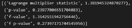
Для удобства создадим пользовательскую функцию Breush_Pagan_test:
def Breush_Pagan_test(
    model_fit,
    p_level: float=0.95,
    model_name=''):

    a_level = 1 - p_level

    # реализация теста
    test = sms.het_breuschpagan(model_fit.resid, model_fit.model.exog)
    name = ['Lagrange_multiplier_statistic', 'p_calc_LM', 'F_statistic', 'p_calc']
    test_result = lzip(name, test)    # распаковка результатов теста
    # расчетное значение статистики теста множителей Лагранжа
    LM_calc_tuple = test_result[0]
    Lagrange_multiplier_statistic = LM_calc_tuple[1]
    # расчетный уровень значимости статистики теста множителей Лагранжа
    p_calc_LM_tuple = test_result[1]
    p_calc_LM = p_calc_LM_tuple[1]
    # расчетное значение F-статистики гипотезы о том, что дисперсия ошибки не зависит от x
    F_calc_tuple = test_result[2]
    F_statistic = F_calc_tuple[1]
    # расчетный уровень значимости F-статистики
    p_calc_tuple = test_result[3]
    p_calc = p_calc_tuple[1]
    # вывод
    conclusion_test = 'heteroscedasticity' if p_calc < a_level else 'not heteroscedasticity'

    # вывод
    conclusion_test = 'heteroscedasticity' if p_calc < a_level else 'not heteroscedasticity'

    result = pd.DataFrame({
        'test': ('Breush-Pagan test'),
        'p_level': (p_level),
        'a_level': (a_level),
        'Lagrange_multiplier_statistic': (Lagrange_multiplier_statistic),
        'p_calc_LM': (p_calc_LM),
        'p_calc_LM < a_level': (p_calc_LM < a_level),
        'F_statistic': (F_statistic),
        'p_calc': (p_calc),
        'p_calc < a_level': (p_calc < a_level),
        'heteroscedasticity_check': (conclusion_test)
        },
        index=[model_name])

    return result

Breush_Pagan_test(result_linear_ols, p_level=0.95, model_name='linear_ols')
Тест Уайта (White test)
# тест Уайта (White test)
name = ["Lagrange multiplier statistic", "p-value", "f-value", "f p-value"]
test = sms.het_white(result_linear_ols.resid, result_linear_ols.model.exog)
lzip(name, test)
Для удобства создадим пользовательскую функцию White_test:
def White_test(
    model_fit,
    p_level: float=0.95,
    model_name=''):

    a_level = 1 - p_level

    # реализация теста
    test = sms.het_white(model_fit.resid, model_fit.model.exog)
    name = ['Lagrange_multiplier_statistic', 'p_calc_LM', 'F_statistic', 'p_calc']
    test_result = lzip(name, test)    # распаковка результатов теста
    # расчетное значение статистики теста множителей Лагранжа
    LM_calc_tuple = test_result[0]
    Lagrange_multiplier_statistic = LM_calc_tuple[1]
    # расчетный уровень значимости статистики теста множителей Лагранжа
    p_calc_LM_tuple = test_result[1]
    p_calc_LM = p_calc_LM_tuple[1]
    # расчетное значение F-статистики гипотезы о том, что дисперсия ошибки не зависит от x
    F_calc_tuple = test_result[2]
    F_statistic = F_calc_tuple[1]
    # расчетный уровень значимости F-статистики
    p_calc_tuple = test_result[3]
    p_calc = p_calc_tuple[1]
    # вывод
    conclusion_test = 'heteroscedasticity' if p_calc < a_level else 'not heteroscedasticity'

    # вывод
    conclusion_test = 'heteroscedasticity' if p_calc < a_level else 'not heteroscedasticity'

    result = pd.DataFrame({
        'test': ('White test'),
        'p_level': (p_level),
        'a_level': (a_level),
        'Lagrange_multiplier_statistic': (Lagrange_multiplier_statistic),
        'p_calc_LM': (p_calc_LM),
        'p_calc_LM < a_level': (p_calc_LM < a_level),
        'F_statistic': (F_statistic),
        'p_calc': (p_calc),
        'p_calc < a_level': (p_calc < a_level),
        'heteroscedasticity_check': (conclusion_test)
        },
        index=[model_name])

    return result

White_test(result_linear_ols, p_level=0.95, model_name='linear_ols')
Объединим результаты всех тестов гетероскедастичность в один DataFrame:
Goldfeld_Quandt_test_df = Goldfeld_Quandt_test(result_linear_ols, p_level=0.95, model_name='linear_ols')
Breush_Pagan_test_df = Breush_Pagan_test(result_linear_ols, p_level=0.95, model_name='linear_ols')
White_test_df = White_test(result_linear_ols, p_level=0.95, model_name='linear_ols')

heteroscedasticity_tests_df = pd.concat([Breush_Pagan_test_df, White_test_df, Goldfeld_Quandt_test_df])
display(heteroscedasticity_tests_df)
Выводы
Итак, мы провели статистический анализ регрессионной модели и установили:
-
исходные данные имеют нормальное распределение;
-
между переменными имеется весьма сильная корреляционная связь;
-
регрессионная модель хорошо аппроксимирует фактические данные;
-
остатки модели имеют нормальное распределение;
-
регрессионная модель адекватна по критерию Фишера;
-
коэффициент детерминации значим по критеию Фишера;
-
коэффициенты регрессии значимы по критерию Стьюдента;
-
гетероскедастичность отсутствует.
Применительно к рассматриваемой задаче выполнять проверку автокорреляции не имеет особого смысла из-за особенностей исходных данных (результаты замеров прочности бетона на разных участках здания).
Про статистический анализ регрессионных моделей с помощью statsmodels— см. еще https://www.statsmodels.org/stable/examples/notebooks/generated/regression_diagnostics.html.
Доверительные интервалы регрессионной модели
Для регрессионных моделей определяют доверительные интервалы двух видов [3, с.184-192; 4, с.172; 8, с.205-209]:
-
Доверительный интервал средних значений переменной Y.
-
Доверительный интервал индивидуальных значений переменной Y.
При этом размер доверительного интервала для индивидуальных значений больше, чем для средних значений.
Доверительные интервалы регрессионных моделей (ДИРМ) могут быть найдены разными способами:
-
непосредственно путем расчетов по формулам (см., например, https://habr.com/ru/post/558158/);
-
с использованием инструментария библиотеки statsmodels (см., например, https://www.stackfinder.ru/questions/17559408/confidence-and-prediction-intervals-with-statsmodels).
Разбререм более подробно способ с использованием библиотеки statsmodels. Прежде всего, с помощью свойства summary_table класса statsmodels.stats.outliers_influence.OLSInfluence (https://www.statsmodels.org/stable/generated/statsmodels.stats.outliers_influence.OLSInfluence.html?highlight=olsinfluence) мы можем получить таблицу данных, содержащую необходимую нам информацию:
-
Dep Var Population — фактические значения переменной Y;
-
Predicted Value — предсказанные значения переменной Y по по регрессионной модели;
-
Std Error Mean Predict — среднеквадратическая ошибка предсказанного среднего;
-
Mean ci 95% low и Mean ci 95% upp — границы доверительного интервала средних значений переменной Y;
-
Predict ci 95% low и Predict ci 95% upp — границы доверительного интервала индивидуальных значений переменной Y;
-
Residual — остатки регрессионной модели;
-
Std Error Residual — среднеквадратическая ошибка остатков;
-
Student Residual — стьюдентизированные остатки (подробнее см. http://statistica.ru/glossary/general/studentizirovannie-ostatki/);
-
Cook’s D — Расстояние Кука (Cook’s distance) — оценивает эффект от удаления одного (рассматриваемого) наблюдения; наблюдение считается выбросом, если Di > 4/n (более подробно — см.https://translated.turbopages.org/proxy_u/en-ru.ru.f584ceb5-63296427-aded8f31-74722d776562/https/en.wikipedia.org/wiki/Cook’s_distance, http://www.machinelearning.ru/wiki/index.php?title=Расстояние_Кука).
from statsmodels.stats.outliers_influence import summary_table
st, data, ss2 = summary_table(result_linear_ols, alpha=0.05)
print(st, 'n', type(st))
В нашем случае критическое значение расстояния Кука равно:
print(f'D_crit = 4/n = {4/result_linear_ols.nobs}')![]()
то есть выбросов, смещающих оценки коэффициентов регрессии, не наблюдается.
Мы получили данные как класс statsmodels.iolib.table.SimpleTable. Свойство data преобразует данные в список. Далее для удобства работы преобразуем данные в DataFrame:
st_data_df = pd.DataFrame(st.data)Будем использовать данный DataFrame в дальнейшем, несколько преобразуем его:
-
изменим наименование столбцов (с цифр на названия показателей из таблицы summary_table)
-
удалим строки с текстовыми значениями
-
изменим индекс
-
добавим новый столбец — значения переменной X
-
отсортируем по возрастанию значений переменной X (это необходимо, чтобы графики границ доверительных интервалов выглядели как линии)
st_df = st_data_df.copy()
# изменим наименования столбцов
str = st_df.iloc[0,0:] + ' ' + st_df.iloc[1,0:]
st_df = st_df.rename(str, axis='columns')
# удалим строки 0, 1
st_df = st_df.drop([0,1])
# изменим индекс
st_df = st_df.set_index(np.arange(0, result_linear_ols.nobs))
# добавим новый столбец - значения переменной X
st_df.insert(1, 'X', X)
# отсортируем по возрастанию значений переменной X
st_df = st_df.sort_values(by='X')

display(st_df)
С помощью полученных данных мы можем построить график регрессионной модели с доверительными интервалами:
# создание рисунка (Figure) и области рисования (Axes)
fig, axes = plt.subplots(figsize=(297/INCH, 210/INCH))
# заголовок рисунка (Figure)
title_figure = Task_Project
fig.suptitle(title_figure, fontsize = 16)
# заголовок области рисования (Axes)
title_axes = 'Линейная регрессионная модель'
axes.set_title(title_axes, fontsize = 14)
# фактические данные
sns.scatterplot(
    x=st_df['X'], y=st_df['Dep Var Population'],
    label='фактические данные',
    s=50,
    color='red',
    ax=axes)
# график регрессионной модели
label_legend_regr_model=f'линейная регрессия Y = {b0:.3f} + {b1:.4f}*X'
sns.lineplot(
    x=st_df['X'], y=st_df['Predicted Value'],
    label=label_legend_regr_model,
    color='blue',
    ax=axes)
# доверительный интервал средних значений переменной Y
Mean_ci_low = st_df['Mean ci 95% low']
plt.plot(
    st_df['X'], Mean_ci_low,
    color='magenta', linestyle='--', linewidth=1,
    label='доверительный интервал средних значений Y')
Mean_ci_upp = st_df['Mean ci 95% upp']
plt.plot(
    st_df['X'], Mean_ci_upp,
    color='magenta', linestyle='--', linewidth=1)
# доверительный интервал индивидуальных значений переменной Y
Predict_ci_low = st_df['Predict ci 95% low']
plt.plot(
    st_df['X'], Predict_ci_low,
    color='orange', linestyle='-.', linewidth=2,
    label='доверительный интервал индивидуальных значений Y')
Predict_ci_upp = st_df['Predict ci 95% upp']
plt.plot(
    st_df['X'], Predict_ci_upp,
    color='orange', linestyle='-.', linewidth=2)

axes.set_xlabel(Variable_Name_X)
axes.set_ylabel(Variable_Name_Y)
axes.legend(prop={'size': 12})
plt.show()
Однако, мы получили данные о границах доверительных интервалов регрессионной модели только в пределах области фактических значений переменной X. Как быть, если мы хотим распространить прогноз за пределы этой области?
Прогнозирование
Под прогнозированием мы в данном случае будем понимать определение значений переменной Y и доверительных интервалов для ее средних и индивидуальных значений при заданном X. По сути, нам предстоит построить аналог рассмотренной выше таблицы summary_table, только с другими значениями X, причем эти значения могут выходить за пределы тех значений, которые использовались нами для построения регрессии.
Методика расчета доверительных интервалов регрессионных моделей разобрана в статье «Python, корреляция и регрессия: часть 4» (https://habr.com/ru/post/558158/), всем рекомендую ознакомиться.
Найти прогнозные значения Y не представляет труда, так как ранее мы уже формализовали модель в виде лямбда-функции, а вот для построения доверительных интервалов придется выполнить расчеты по формулам. Для этого создадим пользовательскую функцию regression_pair_predict, которая в случае парной регрессии (pair regression) для заданного значения X возвращает:
-
прогнозируемое по регрессионной модели значение y_calc
-
доверительный интервал [y_calc_mean_ci_low, y_calc_mean_ci_upp] средних значений переменной Y
-
доверительный интервал [y_calc_predict_ci_low, y_calc_predict_ci_upp] индивидуальных значений переменной Y
Алгоритм расчета доверительных интервалов для множественной регрессии (multiple regression) отличается и в данном обзоре не рассматривается (рассмотрим в дальнейшем).
Про прогнозирование с помощью регрессионных моделей — см.также:
-
https://www.statsmodels.org/stable/generated/statsmodels.regression.linear_model.RegressionResults.predict.html?highlight=predict#statsmodels.regression.linear_model.RegressionResults.predict
-
How to Make Predictions Using Regression Model in Statsmodels
-
https://www.statsmodels.org/stable/examples/notebooks/generated/predict.html
def regression_pair_predict(
    x_in,
    model_fit,
    regression_model,
    p_level: float=0.95):

    a_level = 1 - p_level

    X = pd.DataFrame(model_fit.model.exog)[1].values    # найти лучшее решение
    Y = model_fit.model.endog

    # вспомогательные величины
    n = int(result_linear_ols.nobs)
    SSE = model_fit.ssr    # SSE (Sum of Squared Error)
    dfE = n - p - 1
    MSE = SSE / dfE    # остаточная дисперсия

    Xmean = np.mean(X)
    SST_X = np.sum([(X[i] - Xmean)**2 for i in range(0, n)])

    t_table = sci.stats.t.ppf((1 + p_level)/2 , dfE)
    S2_y_calc_mean = MSE * (1/n + (x_in - Xmean)**2 / SST_X)
    S2_y_calc_predict = MSE * (1 + 1/n + (x_in - Xmean)**2 / SST_X)

    # прогнозируемое значение переменной Y
    y_calc=regression_model(x_in)
    # доверительный интервал средних значений переменной Y
    y_calc_mean_ci_low = y_calc - t_table*sqrt(S2_y_calc_mean)
    y_calc_mean_ci_upp = y_calc + t_table*sqrt(S2_y_calc_mean)
    # доверительный интервал индивидуальных значений переменной Y
    y_calc_predict_ci_low = y_calc - t_table*sqrt(S2_y_calc_predict)
    y_calc_predict_ci_upp = y_calc + t_table*sqrt(S2_y_calc_predict)

    result = y_calc, y_calc_mean_ci_low, y_calc_mean_ci_upp, y_calc_predict_ci_low, y_calc_predict_ci_upp

    return result
Сравним результаты расчета доверительных интервалов разными способами — с использованием функции regression_pair_predict и средствами statsmodels, для этого сформируем DaraFrame с новыми данными:
regression_pair_predict_df = pd.DataFrame(
    [regression_pair_predict(elem, result_linear_ols, regression_model=Y_calc) for elem in st_df['X'].values],
    columns=['y_calc', 'y_calc_mean_ci_low', 'y_calc_mean_ci_upp', 'y_calc_predict_ci_low', 'y_calc_predict_ci_upp'])
regression_pair_predict_df.insert(0, 'X', st_df['X'].values)
display(regression_pair_predict_df)
Видим, что результаты расчетов идентичны, следовательно мы можем использовать функцию regression_pair_predict для прогнозирования.
def graph_regression_pair_predict_plot_sns(
    model_fit,
    regression_model_in,
    Xmin=None, Xmax=None, Nx=10,
    Ymin_graph=None, Ymax_graph=None,
    title_figure=None, title_figure_fontsize=18,
    title_axes=None, title_axes_fontsize=16,
    x_label=None,
    y_label=None,
    label_fontsize=14, tick_fontsize=12,
    label_legend_regr_model='', label_legend_fontsize=12,
    s=50, linewidth_regr_model=2,
    graph_size=(297/INCH, 210/INCH),
    result_output=True,
    file_name=None):

    # фактические данные
    X = pd.DataFrame(model_fit.model.exog)[1].values    # найти лучшее решение
    Y = model_fit.model.endog
    X = np.array(X)
    Y = np.array(Y)

    # границы
    if not(Xmin) and not(Xmax):
        Xmin=min(X)
        Xmax=max(X)
        Xmin_graph=min(X)*0.99
        Xmax_graph=max(X)*1.01
    else:
        Xmin_graph=Xmin
        Xmax_graph=Xmax

    if not(Ymin_graph) and not(Ymax_graph):
        Ymin_graph=min(Y)*0.99
        Ymax_graph=max(Y)*1.01

    # формируем DataFrame данных
    Xcalc = np.linspace(Xmin, Xmax, num=Nx)
    Ycalc = regression_model_in(Xcalc)

    result_df = pd.DataFrame(
        [regression_pair_predict(elem, model_fit, regression_model=regression_model_in) for elem in Xcalc],
        columns=['y_calc', 'y_calc_mean_ci_low', 'y_calc_mean_ci_upp', 'y_calc_predict_ci_low', 'y_calc_predict_ci_upp'])
    result_df.insert(0, 'x_calc', Xcalc)

    # заголовки графика
    fig, axes = plt.subplots(figsize=graph_size)
    fig.suptitle(title_figure, fontsize = title_figure_fontsize)
    axes.set_title(title_axes, fontsize = title_axes_fontsize)

    # фактические данные
    sns.scatterplot(
        x=X, y=Y,
        label='фактические данные',
        s=s,
        color='red',
        ax=axes)

    # график регрессионной модели
    sns.lineplot(
        x=Xcalc, y=Ycalc,
        color='blue',
        linewidth=linewidth_regr_model,
        legend=True,
        label=label_legend_regr_model,
        ax=axes)

    # доверительный интервал средних значений переменной Y
    Mean_ci_low = result_df['y_calc_mean_ci_low']
    plt.plot(
        result_df['x_calc'], Mean_ci_low,
        color='magenta', linestyle='--', linewidth=1,
        label='доверительный интервал средних значений Y')

    Mean_ci_upp = result_df['y_calc_mean_ci_upp']
    plt.plot(
        result_df['x_calc'], Mean_ci_upp,
        color='magenta', linestyle='--', linewidth=1)

    # доверительный интервал индивидуальных значений переменной Y
    Predict_ci_low = result_df['y_calc_predict_ci_low']
    plt.plot(
        result_df['x_calc'], Predict_ci_low,
        color='orange', linestyle='-.', linewidth=2,
        label='доверительный интервал индивидуальных значений Y')

    Predict_ci_upp = result_df['y_calc_predict_ci_upp']
    plt.plot(
        result_df['x_calc'], Predict_ci_upp,
        color='orange', linestyle='-.', linewidth=2)


    axes.set_xlim(Xmin_graph, Xmax_graph)
    axes.set_ylim(Ymin_graph, Ymax_graph)
    axes.set_xlabel(x_label, fontsize = label_fontsize)
    axes.set_ylabel(y_label, fontsize = label_fontsize)
    axes.tick_params(labelsize = tick_fontsize)
    #axes.tick_params(labelsize = tick_fontsize)
    axes.legend(prop={'size': label_legend_fontsize})

    plt.show()
    if file_name:
        fig.savefig(file_name, orientation = "portrait", dpi = 300)

    if result_output:
        return result_df
    else:
        return

graph_regression_pair_predict_plot_sns(
    model_fit=result_linear_ols,
    regression_model_in=Y_calc,
    Xmin=Xmin_graph-300, Xmax=Xmax_graph+200, Nx=25,
    Ymin_graph=Ymin_graph-5, Ymax_graph=Ymax_graph+5,
    title_figure=Task_Project, title_figure_fontsize=16,
    title_axes='Линейная регрессионная модель', title_axes_fontsize=14,
    x_label=Variable_Name_X,
    y_label=Variable_Name_Y,
    label_legend_regr_model=f'линейная регрессия Y = {b0:.3f} + {b1:.4f}*X',
    s=50,
    result_output=True,
    file_name='graph/regression_plot_lin.png')

Выводы и рекомендации
Исследована зависимость показаний ультразвукового прибора «ПУЛЬСАР-2.1» (X) и результатов замера прочности бетона (методом отрыва со скалыванием) склерометром ИПС-МГ4.03 (Y).
Между переменными имеется весьма сильная линейная корреляционная связь. Получена регрессионная модель:
Y = b0 + b1∙X = -21.3741 + 0.0129∙X
Модель хорошо аппроксимирует фактические данные, является адекватной, значимой и может использоваться для предсказания прочности бетона.
Также построен график прогноза с доверительными интервалами.
ИТОГИ
Итак, мы рассмотрели все этапы регрессионного анализа в случае простой линейной регрессии (simple linear regression) с использованием библиотеки statsmodels на конкретном практическом примере; подробно остановились на статистическом анализа модели с проверкой гипотез; также предложен ряд пользовательских функций, облегчающих работу исследователя и уменьшающих размер программного кода.
Конечно, мы разобрали далеко не все вопросы анализа регрессионных моделей и возможности библиотеки statsmodels применительно к simple linear regression, в частности статистики влияния (Influence Statistics), инструмент Leverage, анализ стьюдентизированных остатков и пр. — это темы для отдельных обзоров.
Исходный код находится в моем репозитории на GitHub.
Надеюсь, данный обзор поможет специалистам DataScience в работе.
Introduction
In the previous chapter, we studied machine learning and some key terms associated with it.
From this chapter onwards, we will start with learning and implementing machine learning algorithms. So in that series, in this chapter, we will start with Linear Regression.
Note:
if you can correlate anything with yourself or your life, there are greater chances of understanding the concept. So try to understand everything by relating it to humans.
What is Regression and Why is it called so?
Regression is an ML algorithm that can be trained to predict real numbered outputs; like temperature, stock price, etc. Regression is based on a hypothesis that can be linear, quadratic, polynomial, non-linear, etc. The hypothesis is a function based on some hidden parameters and input values. In the training phase, the hidden parameters are optimized w.r.t. the input values presented in the training. The process that does the optimization is the gradient descent algorithm. You also need a Back-propagation algorithm that can be used to compute the gradient at each layer, If you are using neural networks. Once the hypothesis parameters got trained (when they gave the least error during the training), then the same hypothesis with the trained parameters is used with new input values to predict outcomes that will be again real values.
Types of Regression
1. Linear regression is used for predictive analysis. Linear regression is a linear approach for modeling the relationship between the criterion or the scalar response and the multiple predictors or explanatory variables. Linear regression focuses on the conditional probability distribution of the response given the values of the predictors. For linear regression, there is a danger of overfitting. The formula for linear regression is Y’ = bX + A.
2. Logistic regression is used when the dependent variable is dichotomous. Logistic regression estimates the parameters of a logistic model and is a form of binomial regression. Logistic regression is used to deal with data that has two possible criteria and the relationship between the criteria and the predictors. The equation for logistic regression is l =  .
.
3. Polynomial regression is used for curvilinear data. Polynomial regression is fit with the method of least squares. The goal of regression analysis to model the expected value of a dependent variable y in regards to the independent variable x. The equation for polynomial regression is l = 
4. Stepwise regression is used for fitting regression models with predictive models. It is carried out automatically. With each step, the variable is added or subtracted from the set of explanatory variables. The approaches for stepwise regression are forward selection, backward elimination, and bidirectional elimination. The formula for stepwise regression is 
5. Ridge regression is a technique for analyzing multiple regression data. When multicollinearity occurs, least squares estimates are unbiased. A degree of bias is added to the regression estimates, and a result, ridge regression reduces the standard errors. The formula for ridge regression is 
6. Lasso regression is a regression analysis method that performs both variable selection and regularization. Lasso regression uses soft thresholding. Lasso regression selects only a subset of the provided covariates for use in the final model. Lasso regression is:  .
.
7. ElasticNet regression is a regularized regression method that linearly combines the penalties of the lasso and ridge methods. ElasticNet regression is used to support vector machines, metric learning, and portfolio optimization. The penalty function is given by: 
8. Support Vector regression is a regression method where we identify a hyperplane with maximum margin such that the maximum number of data points are within that margin. SVRs are almost similar to the SVM classification algorithm. Instead of minimizing the error rate as in simple linear regression, we try to fit the error within a certain threshold. Our objective in SVR is to basically consider the points that are within the margin. Our best fit line is the hyperplane that has the maximum number of points.
9. Decision Tree regression is a regression where the ID3 algorithm can be used to identify the splitting node by reducing the standard deviation (in classification information gain is used).
A decision tree is built by partitioning the data into subsets containing instances with similar values (homogenous). Standard deviation is used to calculate the homogeneity of a numerical sample. If the numerical sample is completely homogeneous, its standard deviation is zero.
10. Random Forest regression is an ensemble approach where we take into account the predictions of several decision regression trees.
- Select K random points
- Identify n where n is the number of decision tree regressors to be created. Repeat steps 1 and 2 to create several regression trees.
- The average of each branch is assigned to the leaf node in each decision tree.
- To predict output for a variable, the average of all the predictions of all decision trees are taken into consideration.
Random Forest prevents overfitting (which is common in decision trees) by creating random subsets of the features and building smaller trees using these subsets.
Key Terms
1. Estimator
A formula or algorithm for generating estimates of parameters, given relevant data.
2. Bias
An estimate is unbiased if its expectation equals the value of the parameter being estimated; otherwise, it is biased.
3.Efficiency
An estimator A is more efficient than an estimator B if A has a smaller sampling variance — that is, if the particular values generated by A are more tightly clustered around their expectation.
4. Consistency
An estimator is consistent if the estimates it produces converge on the true parameter value as the sample size increases without limit. Consider an estimator that produces estimates θ^ of some parameter θ, and let ^ denote a small number. If the estimator is consistent, we can make the probability as close to 1.0 as we like or as small as we like by drawing a sufficiently large sample. Note that a biased estimator may nonetheless be consistent if the bias tends to zero in the limit. Conversely, an unbiased estimator may be inconsistent if its sampling variance fails to shrink appropriately as the sample size increases.
5. Standard error of the Regression (SER)
An estimate of the standard deviation of the error term in a regression model.
6. R-squared
A standardized measure of the goodness of fit for a regression model.
7. Standard error of regression coefficient
An estimate of the standard deviation of the sampling distribution for the coefficient in question.
8. P-value
The probability, supposing the null hypothesis to be true, of drawing sample data that are as adverse to the null as the data are actually drawn, or more so. When a small p-value is found, the two possibilities are that we happened to draw a low-probability unrepresentative sample or that the null hypothesis is in fact false.
9. Significance level
For a hypothesis test, this is the smallest p-value for which we will not reject the null hypothesis. If we choose a significance level of 1%, we’re saying that we’ll reject the null if and only if the p-value for the test is less than 0.01. The significance level is also the probability of making a type 1 error (that is, rejecting a true null hypothesis).
10. T-test
The t-test (or z-test, which is the same thing asymptotically) is a common test for the null hypothesis that a particular regression parameter, βi, has some specific value (commonly zero, but generically βH0).
11. F-test
A common procedure for jointly testing a set of linear restrictions on a regression model.
12. Multicollinearity
A situation where there is a high degree of correlation among the independent variables in a regression model — or, more generally, where some of the Xs are close to being linear combinations of other Xs. Symptoms include large standard errors and the inability to produce precise parameter estimates. This is not a serious problem if one is primarily interested in forecasting; it is a problem is one is trying to estimate causal influences.
13. Omitted variable bias
Bias in the estimation of regression parameters that arises when a relevant independent variable is omitted from a model and the omitted variable is correlated with one or more of the included variables.
14. Log variables
A common transformation permits the estimation of a nonlinear model using OLS to substitute the natural log of a variable for the level of that variable. This can be done for the dependent variable and/or one or more independent variables. A key point to remember about logs is that for small changes, the change in the log of a variable is a good approximation to the proportional change in the variable itself. For example, if log(y) changes by 0.04, y changes by about 4%.
15. Quadratic terms
Another common transformation. When both xi and x^2_i are included as regressors, it is important to remember that the estimated effect of xi on y is given by the derivative of the regression equation with respect to xi. If the coefficient on xi is β and the coefficient on x 2 i is γ, the derivative is β + 2γ xi.
16. Interaction terms
Pairwise products of the «original» independent variables. The inclusion of interaction terms in a regression allows for the possibility that the degree to which xi affects y depends on the value of some other variable x j. In other words, x j modulates the effect of xi on y. For example, the effect of experience on wages (xi) might depend on the gender (x j) of the worker.
17. Independent Variable
An independent variable is a variable that is changed or controlled in a scientific experiment to test the effects on the dependent variable.
18. Dependent Variable
A dependent variable is a variable being tested and measured in a scientific experiment. The dependent variable is ‘dependent’ on the independent variable. As the experimenter changes the independent variable, the effect on the dependent variable is observed and recorded.
19. Regularization
There are extensions of the training of the linear model called regularization methods. These seek to both minimize the sum of the squared error of the model on the training data (using ordinary least squares) but also to reduce the complexity of the model (like the number or absolute size of the sum of all coefficients in the model).
Gradient Descent
Gradient descent is an optimization algorithm used to minimize some function by iteratively moving in the direction of steepest descent as defined by the negative of the gradient. In machine learning, we use gradient descent to update the parameters of our model. Parameters refer to coefficients in Linear Regression and weights in neural networks.
1. Learning Rate
The size of these steps is called the learning rate. With a high learning rate, we can cover more ground each step, but we risk overshooting the lowest point since the slope of the hill is constantly changing. With a very low learning rate, we can confidently move in the direction of the negative gradient since we are recalculating it so frequently. A low learning rate is more precise, but calculating the gradient is time-consuming, so it will take us a very long time to get to the bottom.
2. Cost Function
A Loss Function or Cost Function tells us “how good” our model is at making predictions for a given set of parameters. The cost function has its own curve and its own gradients. The slope of this curve tells us how to update our parameters to make the model more accurate.

Python Implementation of Gradient Descent
- def update_weights(m, b, X, Y, learning_rate):
- m_deriv = 0
- b_deriv = 0
- N = len(X)
- for i in range(N):
- m_deriv += —2*X[i] * (Y[i] — (m*X[i] + b))
- b_deriv += —2*(Y[i] — (m*X[i] + b))
- m -= (m_deriv / float(N)) * learning_rate
- b -= (b_deriv / float(N)) * learning_rate
- return m, b
Remembering Variables With DRYMIX
When results are plotted in graphs, the convention is to use the independent variable as the x-axis and the dependent variable as the y-axis. The DRY MIX acronym can help keep the variables straight:
- D is the dependent variable
- R is the responding variable
- Y is the axis on which the dependent or responding variable is graphed (the vertical axis)
- M is the manipulated variable or the one that is changed in an experiment
- I is the independent variable
- X is the axis on which the independent or manipulated variable is graphed (the horizontal axis)
Simple Linear Regression Model
The simple linear regression model is represented like this: y = (β0 +β1 + Ε)
By mathematical convention, the two factors that are involved in simple linear regression analysis are designated x and y. The equation that describes how y is related to x is known as the regression model. The linear regression model also contains an error term that is represented by Ε, or the Greek letter epsilon. The error term is used to account for the variability in y that cannot be explained by the linear relationship between x and y. There also parameters that represent the population being studied. These parameters of the model are represented by (β0+β1x).
The simple linear regression equation is graphed as a straight line.
The simple linear regression equation is represented like this: Ε(y) = (β0 +β1*x)
- β0 is the y-intercept of the regression line.
- β1 is the slope.
- Ε(y) is the mean or expected value of y for a given value of x.
A regression line can show a positive linear relationship, a negative linear relationship, or no relationship.
- If the graphed line in a simple linear regression is flat (not sloped), there is no relationship between the two variables.
- If the regression line slopes upward with the lower end of the line at the y-intercept (axis) of the graph, and the upper end of the line extending upward into the graph field, away from the x-intercept (axis) a positive linear relationship exists.
- If the regression line slopes downward with the upper end of the line at the y-intercept (axis) of the graph, and the lower end of the line extending downward into the graph field, toward the x-intercept (axis) a negative linear relationship exists.
y = β0 +β1*x

Important Note
1. Regression analysis is not used to interpret cause-and-effect relationships( a mechanism where one event makes another event happen, i.e each event is dependent on one-another) between variables. Regression analysis can, however, indicate how variables are related or to what extent variables are associated with each other.
2. It is also known as bivariate regression or regression analysis
Sum of Square Errors
This is the sum of differences between the points and the regression line. It can serve as a measure of how well the line fits the data.
![]()
Standard Estimate of Errors
The mean error is equal to zero. If se(sigma_epsilon) is small the errors tend to be close to zero (close to the mean error). Then, the model fits the data well. Therefore, we can use se as a measure of the suitability of using a linear model. An estimator of se is given by se(sigma_epsilon)
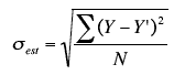
Coefficient of Determination
To measure the strength of the linear relationship we use the coefficient of determination. R^2 takes on any value between zero and one.
- R^2 = 1: Perfect match between the line and the data points.
- R^2 = 0: There is no linear relationship between x and y.
Simple Linear Regression Example
Let’s take the example of Housing Price Prediction, the data that I am using is KC House Prices. Feel free to use any dataset, there some very good datasets available on kaggle and with Google Colab.
- import pandas as pd
- df = pd.read_csv(«kc_house_data.csv»)
- df.describe()
Output

From the above data, we can see that we have a lot of tables, but simple linear regression can only process two columns, so we select the «price» and «sqrt_living». Here we will take the first 100 rows for our demonstration.
Before fitting the data let’s analyze the data:
- import seaborn as sns
- df = pd.read_csv(«kc_house_data.csv»)
- sns.distplot(df[‘price’][1:100])
Output

- import seaborn as sns
- df = pd.read_csv(«kc_house_data.csv»)
- sns.distplot(df[‘sqrt_living’][1:100])
Output

1. Demo using Numpy
In the below code, we will just use numpy to perform linear regression.
- import pandas as pd
- import numpy as np
- import matplotlib.pyplot as plt
- %matplotlib inline
- def estimate_coef(x, y):
- n = np.size(x)
- m_x, m_y = np.mean(x), np.mean(y)
- SS_xy = np.sum(y*x) — n*m_y*m_x
- SS_xx = np.sum(x*x) — n*m_x*m_x
- b_1 = SS_xy / SS_xx
- b_0 = m_y — b_1*m_x
- return(b_0, b_1)
- def plot_regression_line(x, y, b):
- plt.scatter(x, y, color = «m»,
- marker = «o», s = 30)
- y_pred = b[0] + b[1]*x
- plt.plot(x, y_pred, color = «g»)
- plt.xlabel(‘x’)
- plt.ylabel(‘y’)
- plt.show()
- def main():
- df = pd.read_csv(«kc_house_data.csv»)
- y= df[‘price’][1:100]
- x= df[‘sqft_living’][1:100]
- plt.scatter(x, y)
- plt.xlabel(‘x’)
- plt.ylabel(‘y’)
- plt.show()
- b = estimate_coef(x, y)
- print(«Estimated coefficients:nb_0 = {} nb_1 = {}».format(b[0], b[1]))
- plot_regression_line(x, y, b)
- if __name__ == «__main__»:
- main()
Output
The input data can be visualized as:

After, executing the code we get the following output
Estimated coefficients: b_0 = 41517.979725295736 b_1 = 229.10249314945074
So the Linear Regression equation becomes :
[price] = 41517.979725795736+ 229.10249374945074*[sqrt_living]
i.e y = b[0] + b[1]*x
Let’s see the final plot with the Regression Line

To predict the values we run the following command:
- print(«For x =100», «the predicted value would be»,(b[1]*100+b[0]))
So the predicted value that we get is 64428.22904024081
Since the machine has to learn, hence would be doing some errors in predicting, so the let’s see what percentage of error it is performing at each given point
- y_diff = y -(b[1]+b[0]*x)
- sns.distplot(y_diff)

2. Demo using Sklearn
In the below code, we will learn how to code linear regression using SkLearn
- import pandas as pd
- import numpy as np
- import matplotlib.pyplot as plt
- import seaborn as sns
- df = pd.read_csv(«kc_house_data.csv»)
- y= df[‘price’][1:100]
- x= df[‘sqft_living’][1:100]
- from sklearn.model_selection import train_test_split
- x_train, x_test, y_train, y_test = train_test_split(x, y, test_size=0.2, random_state=101)
- from sklearn.linear_model import LinearRegression
- lr = LinearRegression()
- x_train = x_train.values.reshape(-1,1)
- lr.fit(x_train, y_train)
- print(«b[0] = «,lr.intercept_)
- print(«b[1] = «,lr.coef_)
- x_test = x_test.values.reshape(-1,1)
- pred = lr.predict(x_test)
- plt.scatter(x_train,y_train)
- y_pred = lr.intercept_ + lr.coef_*x_train
- plt.plot(x_train, y_pred, color = «g»)
- plt.xlabel(‘x’)
- plt.ylabel(‘y’)
- plt.show()
Output

After, executing the code we get the following output
b[0] = 21803.55365770642 b[1] = [232.07541739]
So the Linear Regression equation becomes :
[price] = 21803.55365770642+ 232.07541739*[sqrt_living]
i.e y = b[0] + b[1]*x
Let’s now see a graphical representation between predicted value wrt test set

Since the machine has to learn, hence would be doing some errors in predicting, so the let’s see what percentage of error it is performing at each given point
- sns.distplot((y_test-pred))

3. Demo using TensorFlow
In this, I will not be using «kc_house_data.csv». To make it as simple as possible, I used some dummy data and then I will explain each and everything
- np.random.seed(101)
- tf.set_random_seed(101)
We first set the seed value for both NumPy and TensorFlow. The seed value is used for random number generation.
- x = np.linspace(0, 50, 50)
- y = np.linspace(0, 50, 50)
We now generate dummy data using the NumPy’s linspace function, which generated 50 equally distributed points between 0 and 50
- x += np.random.uniform(-4, 4, 50)
- y += np.random.uniform(-4, 4, 50)
Since the data so generated is too perfect, so we add a liitle bit of uniformaly distributed white noise.
- n = len(x)
- plt.scatter(x, y)
- plt.xlabel(‘x’)
- plt.xlabel(‘y’)
- plt.title(«Training Data»)
- plt.show()
Here, we thus plot the graphical representation of the dummy data.
- X = tf.placeholder(«float»)
- Y = tf.placeholder(«float»)
- W = tf.Variable(np.random.randn(), name = «W»)
- b = tf.Variable(np.random.randn(), name = «b»)
Here we are setting X and Y as the actual training data and the W and b as the trainable data, where:
- W means Weight
- b means bais
- X means the dependent variable
- Y means the independent variable
We have to give initial weights and bias to the model. So, we initialize them with some random values.
- learning_rate = 0.01
- training_epochs = 1000
Here, we assume the learning rate to be 0.01 i.e. the gradient descent value would increase/decrease by 0.01 and we will train the model 1000 times or for 1000 epochs
- y_pred = tf.add(tf.multiply(X, W), b)
- cost = tf.reduce_sum(tf.pow(y_pred-Y, 2)) / (2 * n)
- optimizer = tf.train.GradientDescentOptimizer(learning_rate).minimize(cost)
- init = tf.global_variables_initializer()
Next thing, we have to set the hypothesis, cost function, the optimizer (which will make sure that model is learning on every epoch), and the global variable initializer.
- Since we are using simple linear regression hence the hypothesis is set as:
Depedent_Variable*Weight+Bias or Depedent_Variable*b[1]+b[0]
- We choose the cost function to be mean squared error cost function
- We choose the optimizer as Gradient Descent with the motive of minimizing the cost with given learning rate
- We use TensorFlow’s global variable initialize the global variable so that we can re-use the value of variables
- with tf.Session() as sess:
- sess.run(init)
- for epoch in range(training_epochs):
- for (_x, _y) in zip(x, y):
- sess.run(optimizer, feed_dict = {X : _x, Y : _y})
- if (epoch + 1) % 50 == 0:
- c = sess.run(cost, feed_dict = {X : x, Y : y})
- print(«Epoch», (epoch + 1), «: cost =», c, «W =», sess.run(W), «b =», sess.run(b))
- tf.Session()
we start the TensorFlow session and name the Session as sess. We then initialize all the required variable using the - sess.run(init)
initialize all the required variable using the - for epoch in range(training_epochs)
create a for loop that runs till epoch becomes equal to training_epocs - for (_x, _y) in zip (x,y)
this is used to form a set of values from the given data and then parse through the so formed sets - sess.run(optimizer, feed_dict = {X: _x, Y: _y})
used to run the first optimizer iteration on each the data points - if(epoch+1)%50==0
to break the given iterations into a batch of 50 each - c= sess.run(cost, feed_dict= {X: x, Y: y})
performs the training on the given data points - print(«Epoch»,(epoch+1),»: cost», c, «W =», sess.run(W), «b =», sess.run(b)
print the values after each 50 epochs
- training_cost = sess.run(cost, feed_dict ={X: x, Y: y})
- weight = sess.run(W)
- bias = sess.run(b)
the above code is used to store the values for the next session
- predictions = weight * x + bias
- print(«Training cost =», training_cost, «Weight =», weight, «bias =», bias, ‘n’)
- plt.plot(x, y, ‘ro’, label =‘Original data’)
- plt.plot(x, predictions, label =‘Fitted line’)
- plt.title(‘Linear Regression Result’)
- plt.legend()
- plt.show()
The above code demonstrates how we can use the trained model to predict values
LR_TensorFlow.py
- import numpy as np
- import tensorflow as tf
- import matplotlib.pyplot as plt
- np.random.seed(101)
- tf.set_random_seed(101)
- x = np.linspace(0, 50, 50)
- y = np.linspace(0, 50, 50)
- x += np.random.uniform(-4, 4, 50)
- y += np.random.uniform(-4, 4, 50)
- n = len(x)
- plt.scatter(x, y)
- plt.xlabel(‘x’)
- plt.xlabel(‘y’)
- plt.title(«Training Data»)
- plt.show()
- X = tf.placeholder(«float»)
- Y = tf.placeholder(«float»)
- W = tf.Variable(np.random.randn(), name = «W»)
- b = tf.Variable(np.random.randn(), name = «b»)
- learning_rate = 0.01
- training_epochs = 1000
- y_pred = tf.add(tf.multiply(X, W), b)
- cost = tf.reduce_sum(tf.pow(y_pred-Y, 2)) / (2 * n)
- optimizer = tf.train.GradientDescentOptimizer(learning_rate).minimize(cost)
- init = tf.global_variables_initializer()
- with tf.Session() as sess:
- sess.run(init)
- for epoch in range(training_epochs):
- for (_x, _y) in zip(x, y):
- sess.run(optimizer, feed_dict = {X : _x, Y : _y})
- if (epoch + 1) % 50 == 0:
- c = sess.run(cost, feed_dict = {X : x, Y : y})
- print(«Epoch», (epoch + 1), «: cost =», c, «W =», sess.run(W), «b =», sess.run(b))
- training_cost = sess.run(cost, feed_dict ={X: x, Y: y})
- weight = sess.run(W)
- bias = sess.run(b)
- predictions = weight * x + bias
- print(«Training cost =», training_cost, «Weight =», weight, «bias =», bias, ‘n’)
- plt.plot(x, y, ‘ro’, label =‘Original data’)
- plt.plot(x, predictions, label =‘Fitted line’)
- plt.title(‘Linear Regression Result’)
- plt.legend()
- plt.show()
Output


After, executing the code we get the following output
b[0] = 1.0199214 b[1] = 0.02561676
So the Linear Regression equation becomes :
[y] = 1.0199214+ 1.0199214*[x]
i.e y = b[0] + b[1]*x
Conclusion
In this chapter, we studied regression and simple linear regression.
In the next chapter, we will study the simple logistic regression, which is another type of regression.
Introduction
In the previous chapter, we studied machine learning and some key terms associated with it.
From this chapter onwards, we will start with learning and implementing machine learning algorithms. So in that series, in this chapter, we will start with Linear Regression.
Note:
if you can correlate anything with yourself or your life, there are greater chances of understanding the concept. So try to understand everything by relating it to humans.
What is Regression and Why is it called so?
Regression is an ML algorithm that can be trained to predict real numbered outputs; like temperature, stock price, etc. Regression is based on a hypothesis that can be linear, quadratic, polynomial, non-linear, etc. The hypothesis is a function based on some hidden parameters and input values. In the training phase, the hidden parameters are optimized w.r.t. the input values presented in the training. The process that does the optimization is the gradient descent algorithm. You also need a Back-propagation algorithm that can be used to compute the gradient at each layer, If you are using neural networks. Once the hypothesis parameters got trained (when they gave the least error during the training), then the same hypothesis with the trained parameters is used with new input values to predict outcomes that will be again real values.
Types of Regression
1. Linear regression is used for predictive analysis. Linear regression is a linear approach for modeling the relationship between the criterion or the scalar response and the multiple predictors or explanatory variables. Linear regression focuses on the conditional probability distribution of the response given the values of the predictors. For linear regression, there is a danger of overfitting. The formula for linear regression is Y’ = bX + A.
2. Logistic regression is used when the dependent variable is dichotomous. Logistic regression estimates the parameters of a logistic model and is a form of binomial regression. Logistic regression is used to deal with data that has two possible criteria and the relationship between the criteria and the predictors. The equation for logistic regression is l = .
3. Polynomial regression is used for curvilinear data. Polynomial regression is fit with the method of least squares. The goal of regression analysis to model the expected value of a dependent variable y in regards to the independent variable x. The equation for polynomial regression is l =
4. Stepwise regression is used for fitting regression models with predictive models. It is carried out automatically. With each step, the variable is added or subtracted from the set of explanatory variables. The approaches for stepwise regression are forward selection, backward elimination, and bidirectional elimination. The formula for stepwise regression is
5. Ridge regression is a technique for analyzing multiple regression data. When multicollinearity occurs, least squares estimates are unbiased. A degree of bias is added to the regression estimates, and a result, ridge regression reduces the standard errors. The formula for ridge regression is
6. Lasso regression is a regression analysis method that performs both variable selection and regularization. Lasso regression uses soft thresholding. Lasso regression selects only a subset of the provided covariates for use in the final model. Lasso regression is: .
7. ElasticNet regression is a regularized regression method that linearly combines the penalties of the lasso and ridge methods. ElasticNet regression is used to support vector machines, metric learning, and portfolio optimization. The penalty function is given by:
8. Support Vector regression is a regression method where we identify a hyperplane with maximum margin such that the maximum number of data points are within that margin. SVRs are almost similar to the SVM classification algorithm. Instead of minimizing the error rate as in simple linear regression, we try to fit the error within a certain threshold. Our objective in SVR is to basically consider the points that are within the margin. Our best fit line is the hyperplane that has the maximum number of points.
9. Decision Tree regression is a regression where the ID3 algorithm can be used to identify the splitting node by reducing the standard deviation (in classification information gain is used).
A decision tree is built by partitioning the data into subsets containing instances with similar values (homogenous). Standard deviation is used to calculate the homogeneity of a numerical sample. If the numerical sample is completely homogeneous, its standard deviation is zero.
10. Random Forest regression is an ensemble approach where we take into account the predictions of several decision regression trees.
- Select K random points
- Identify n where n is the number of decision tree regressors to be created. Repeat steps 1 and 2 to create several regression trees.
- The average of each branch is assigned to the leaf node in each decision tree.
- To predict output for a variable, the average of all the predictions of all decision trees are taken into consideration.
Random Forest prevents overfitting (which is common in decision trees) by creating random subsets of the features and building smaller trees using these subsets.
Key Terms
1. Estimator
A formula or algorithm for generating estimates of parameters, given relevant data.
2. Bias
An estimate is unbiased if its expectation equals the value of the parameter being estimated; otherwise, it is biased.
3.Efficiency
An estimator A is more efficient than an estimator B if A has a smaller sampling variance — that is, if the particular values generated by A are more tightly clustered around their expectation.
4. Consistency
An estimator is consistent if the estimates it produces converge on the true parameter value as the sample size increases without limit. Consider an estimator that produces estimates θ^ of some parameter θ, and let ^ denote a small number. If the estimator is consistent, we can make the probability as close to 1.0 as we like or as small as we like by drawing a sufficiently large sample. Note that a biased estimator may nonetheless be consistent if the bias tends to zero in the limit. Conversely, an unbiased estimator may be inconsistent if its sampling variance fails to shrink appropriately as the sample size increases.
5. Standard error of the Regression (SER)
An estimate of the standard deviation of the error term in a regression model.
6. R-squared
A standardized measure of the goodness of fit for a regression model.
7. Standard error of regression coefficient
An estimate of the standard deviation of the sampling distribution for the coefficient in question.
8. P-value
The probability, supposing the null hypothesis to be true, of drawing sample data that are as adverse to the null as the data are actually drawn, or more so. When a small p-value is found, the two possibilities are that we happened to draw a low-probability unrepresentative sample or that the null hypothesis is in fact false.
9. Significance level
For a hypothesis test, this is the smallest p-value for which we will not reject the null hypothesis. If we choose a significance level of 1%, we’re saying that we’ll reject the null if and only if the p-value for the test is less than 0.01. The significance level is also the probability of making a type 1 error (that is, rejecting a true null hypothesis).
10. T-test
The t-test (or z-test, which is the same thing asymptotically) is a common test for the null hypothesis that a particular regression parameter, βi, has some specific value (commonly zero, but generically βH0).
11. F-test
A common procedure for jointly testing a set of linear restrictions on a regression model.
12. Multicollinearity
A situation where there is a high degree of correlation among the independent variables in a regression model — or, more generally, where some of the Xs are close to being linear combinations of other Xs. Symptoms include large standard errors and the inability to produce precise parameter estimates. This is not a serious problem if one is primarily interested in forecasting; it is a problem is one is trying to estimate causal influences.
13. Omitted variable bias
Bias in the estimation of regression parameters that arises when a relevant independent variable is omitted from a model and the omitted variable is correlated with one or more of the included variables.
14. Log variables
A common transformation permits the estimation of a nonlinear model using OLS to substitute the natural log of a variable for the level of that variable. This can be done for the dependent variable and/or one or more independent variables. A key point to remember about logs is that for small changes, the change in the log of a variable is a good approximation to the proportional change in the variable itself. For example, if log(y) changes by 0.04, y changes by about 4%.
15. Quadratic terms
Another common transformation. When both xi and x^2_i are included as regressors, it is important to remember that the estimated effect of xi on y is given by the derivative of the regression equation with respect to xi. If the coefficient on xi is β and the coefficient on x 2 i is γ, the derivative is β + 2γ xi.
16. Interaction terms
Pairwise products of the «original» independent variables. The inclusion of interaction terms in a regression allows for the possibility that the degree to which xi affects y depends on the value of some other variable x j. In other words, x j modulates the effect of xi on y. For example, the effect of experience on wages (xi) might depend on the gender (x j) of the worker.
17. Independent Variable
An independent variable is a variable that is changed or controlled in a scientific experiment to test the effects on the dependent variable.
18. Dependent Variable
A dependent variable is a variable being tested and measured in a scientific experiment. The dependent variable is ‘dependent’ on the independent variable. As the experimenter changes the independent variable, the effect on the dependent variable is observed and recorded.
19. Regularization
There are extensions of the training of the linear model called regularization methods. These seek to both minimize the sum of the squared error of the model on the training data (using ordinary least squares) but also to reduce the complexity of the model (like the number or absolute size of the sum of all coefficients in the model).
Gradient Descent
Gradient descent is an optimization algorithm used to minimize some function by iteratively moving in the direction of steepest descent as defined by the negative of the gradient. In machine learning, we use gradient descent to update the parameters of our model. Parameters refer to coefficients in Linear Regression and weights in neural networks.
1. Learning Rate
The size of these steps is called the learning rate. With a high learning rate, we can cover more ground each step, but we risk overshooting the lowest point since the slope of the hill is constantly changing. With a very low learning rate, we can confidently move in the direction of the negative gradient since we are recalculating it so frequently. A low learning rate is more precise, but calculating the gradient is time-consuming, so it will take us a very long time to get to the bottom.
2. Cost Function
A Loss Function or Cost Function tells us “how good” our model is at making predictions for a given set of parameters. The cost function has its own curve and its own gradients. The slope of this curve tells us how to update our parameters to make the model more accurate.
Python Implementation of Gradient Descent
- def update_weights(m, b, X, Y, learning_rate):
- m_deriv = 0
- b_deriv = 0
- N = len(X)
- for i in range(N):
- m_deriv += —2*X[i] * (Y[i] — (m*X[i] + b))
- b_deriv += —2*(Y[i] — (m*X[i] + b))
- m -= (m_deriv / float(N)) * learning_rate
- b -= (b_deriv / float(N)) * learning_rate
- return m, b
Remembering Variables With DRYMIX
When results are plotted in graphs, the convention is to use the independent variable as the x-axis and the dependent variable as the y-axis. The DRY MIX acronym can help keep the variables straight:
- D is the dependent variable
- R is the responding variable
- Y is the axis on which the dependent or responding variable is graphed (the vertical axis)
- M is the manipulated variable or the one that is changed in an experiment
- I is the independent variable
- X is the axis on which the independent or manipulated variable is graphed (the horizontal axis)
Simple Linear Regression Model
The simple linear regression model is represented like this: y = (β0 +β1 + Ε)
By mathematical convention, the two factors that are involved in simple linear regression analysis are designated x and y. The equation that describes how y is related to x is known as the regression model. The linear regression model also contains an error term that is represented by Ε, or the Greek letter epsilon. The error term is used to account for the variability in y that cannot be explained by the linear relationship between x and y. There also parameters that represent the population being studied. These parameters of the model are represented by (β0+β1x).
The simple linear regression equation is graphed as a straight line.
The simple linear regression equation is represented like this: Ε(y) = (β0 +β1*x)
- β0 is the y-intercept of the regression line.
- β1 is the slope.
- Ε(y) is the mean or expected value of y for a given value of x.
A regression line can show a positive linear relationship, a negative linear relationship, or no relationship.
- If the graphed line in a simple linear regression is flat (not sloped), there is no relationship between the two variables.
- If the regression line slopes upward with the lower end of the line at the y-intercept (axis) of the graph, and the upper end of the line extending upward into the graph field, away from the x-intercept (axis) a positive linear relationship exists.
- If the regression line slopes downward with the upper end of the line at the y-intercept (axis) of the graph, and the lower end of the line extending downward into the graph field, toward the x-intercept (axis) a negative linear relationship exists.
y = β0 +β1*x
Important Note
1. Regression analysis is not used to interpret cause-and-effect relationships( a mechanism where one event makes another event happen, i.e each event is dependent on one-another) between variables. Regression analysis can, however, indicate how variables are related or to what extent variables are associated with each other.
2. It is also known as bivariate regression or regression analysis
Sum of Square Errors
This is the sum of differences between the points and the regression line. It can serve as a measure of how well the line fits the data.
![]()
Standard Estimate of Errors
The mean error is equal to zero. If se(sigma_epsilon) is small the errors tend to be close to zero (close to the mean error). Then, the model fits the data well. Therefore, we can use se as a measure of the suitability of using a linear model. An estimator of se is given by se(sigma_epsilon)
Coefficient of Determination
To measure the strength of the linear relationship we use the coefficient of determination. R^2 takes on any value between zero and one.
- R^2 = 1: Perfect match between the line and the data points.
- R^2 = 0: There is no linear relationship between x and y.
Simple Linear Regression Example
Let’s take the example of Housing Price Prediction, the data that I am using is KC House Prices. Feel free to use any dataset, there some very good datasets available on kaggle and with Google Colab.
- import pandas as pd
- df = pd.read_csv(«kc_house_data.csv»)
- df.describe()
Output
From the above data, we can see that we have a lot of tables, but simple linear regression can only process two columns, so we select the «price» and «sqrt_living». Here we will take the first 100 rows for our demonstration.
Before fitting the data let’s analyze the data:
- import seaborn as sns
- df = pd.read_csv(«kc_house_data.csv»)
- sns.distplot(df[‘price’][1:100])
Output
- import seaborn as sns
- df = pd.read_csv(«kc_house_data.csv»)
- sns.distplot(df[‘sqrt_living’][1:100])
Output
1. Demo using Numpy
In the below code, we will just use numpy to perform linear regression.
- import pandas as pd
- import numpy as np
- import matplotlib.pyplot as plt
- %matplotlib inline
- def estimate_coef(x, y):
- n = np.size(x)
- m_x, m_y = np.mean(x), np.mean(y)
- SS_xy = np.sum(y*x) — n*m_y*m_x
- SS_xx = np.sum(x*x) — n*m_x*m_x
- b_1 = SS_xy / SS_xx
- b_0 = m_y — b_1*m_x
- return(b_0, b_1)
- def plot_regression_line(x, y, b):
- plt.scatter(x, y, color = «m»,
- marker = «o», s = 30)
- y_pred = b[0] + b[1]*x
- plt.plot(x, y_pred, color = «g»)
- plt.xlabel(‘x’)
- plt.ylabel(‘y’)
- plt.show()
- def main():
- df = pd.read_csv(«kc_house_data.csv»)
- y= df[‘price’][1:100]
- x= df[‘sqft_living’][1:100]
- plt.scatter(x, y)
- plt.xlabel(‘x’)
- plt.ylabel(‘y’)
- plt.show()
- b = estimate_coef(x, y)
- print(«Estimated coefficients:nb_0 = {} nb_1 = {}».format(b[0], b[1]))
- plot_regression_line(x, y, b)
- if __name__ == «__main__»:
- main()
Output
The input data can be visualized as:
After, executing the code we get the following output
Estimated coefficients: b_0 = 41517.979725295736 b_1 = 229.10249314945074
So the Linear Regression equation becomes :
[price] = 41517.979725795736+ 229.10249374945074*[sqrt_living]
i.e y = b[0] + b[1]*x
Let’s see the final plot with the Regression Line
To predict the values we run the following command:
- print(«For x =100», «the predicted value would be»,(b[1]*100+b[0]))
So the predicted value that we get is 64428.22904024081
Since the machine has to learn, hence would be doing some errors in predicting, so the let’s see what percentage of error it is performing at each given point
- y_diff = y -(b[1]+b[0]*x)
- sns.distplot(y_diff)
2. Demo using Sklearn
In the below code, we will learn how to code linear regression using SkLearn
- import pandas as pd
- import numpy as np
- import matplotlib.pyplot as plt
- import seaborn as sns
- df = pd.read_csv(«kc_house_data.csv»)
- y= df[‘price’][1:100]
- x= df[‘sqft_living’][1:100]
- from sklearn.model_selection import train_test_split
- x_train, x_test, y_train, y_test = train_test_split(x, y, test_size=0.2, random_state=101)
- from sklearn.linear_model import LinearRegression
- lr = LinearRegression()
- x_train = x_train.values.reshape(-1,1)
- lr.fit(x_train, y_train)
- print(«b[0] = «,lr.intercept_)
- print(«b[1] = «,lr.coef_)
- x_test = x_test.values.reshape(-1,1)
- pred = lr.predict(x_test)
- plt.scatter(x_train,y_train)
- y_pred = lr.intercept_ + lr.coef_*x_train
- plt.plot(x_train, y_pred, color = «g»)
- plt.xlabel(‘x’)
- plt.ylabel(‘y’)
- plt.show()
Output
After, executing the code we get the following output
b[0] = 21803.55365770642 b[1] = [232.07541739]
So the Linear Regression equation becomes :
[price] = 21803.55365770642+ 232.07541739*[sqrt_living]
i.e y = b[0] + b[1]*x
Let’s now see a graphical representation between predicted value wrt test set
Since the machine has to learn, hence would be doing some errors in predicting, so the let’s see what percentage of error it is performing at each given point
- sns.distplot((y_test-pred))
3. Demo using TensorFlow
In this, I will not be using «kc_house_data.csv». To make it as simple as possible, I used some dummy data and then I will explain each and everything
- np.random.seed(101)
- tf.set_random_seed(101)
We first set the seed value for both NumPy and TensorFlow. The seed value is used for random number generation.
- x = np.linspace(0, 50, 50)
- y = np.linspace(0, 50, 50)
We now generate dummy data using the NumPy’s linspace function, which generated 50 equally distributed points between 0 and 50
- x += np.random.uniform(-4, 4, 50)
- y += np.random.uniform(-4, 4, 50)
Since the data so generated is too perfect, so we add a liitle bit of uniformaly distributed white noise.
- n = len(x)
- plt.scatter(x, y)
- plt.xlabel(‘x’)
- plt.xlabel(‘y’)
- plt.title(«Training Data»)
- plt.show()
Here, we thus plot the graphical representation of the dummy data.
- X = tf.placeholder(«float»)
- Y = tf.placeholder(«float»)
- W = tf.Variable(np.random.randn(), name = «W»)
- b = tf.Variable(np.random.randn(), name = «b»)
Here we are setting X and Y as the actual training data and the W and b as the trainable data, where:
- W means Weight
- b means bais
- X means the dependent variable
- Y means the independent variable
We have to give initial weights and bias to the model. So, we initialize them with some random values.
- learning_rate = 0.01
- training_epochs = 1000
Here, we assume the learning rate to be 0.01 i.e. the gradient descent value would increase/decrease by 0.01 and we will train the model 1000 times or for 1000 epochs
- y_pred = tf.add(tf.multiply(X, W), b)
- cost = tf.reduce_sum(tf.pow(y_pred-Y, 2)) / (2 * n)
- optimizer = tf.train.GradientDescentOptimizer(learning_rate).minimize(cost)
- init = tf.global_variables_initializer()
Next thing, we have to set the hypothesis, cost function, the optimizer (which will make sure that model is learning on every epoch), and the global variable initializer.
- Since we are using simple linear regression hence the hypothesis is set as:
Depedent_Variable*Weight+Bias or Depedent_Variable*b[1]+b[0]
- We choose the cost function to be mean squared error cost function
- We choose the optimizer as Gradient Descent with the motive of minimizing the cost with given learning rate
- We use TensorFlow’s global variable initialize the global variable so that we can re-use the value of variables
- with tf.Session() as sess:
- sess.run(init)
- for epoch in range(training_epochs):
- for (_x, _y) in zip(x, y):
- sess.run(optimizer, feed_dict = {X : _x, Y : _y})
- if (epoch + 1) % 50 == 0:
- c = sess.run(cost, feed_dict = {X : x, Y : y})
- print(«Epoch», (epoch + 1), «: cost =», c, «W =», sess.run(W), «b =», sess.run(b))
- tf.Session()
we start the TensorFlow session and name the Session as sess. We then initialize all the required variable using the - sess.run(init)
initialize all the required variable using the - for epoch in range(training_epochs)
create a for loop that runs till epoch becomes equal to training_epocs - for (_x, _y) in zip (x,y)
this is used to form a set of values from the given data and then parse through the so formed sets - sess.run(optimizer, feed_dict = {X: _x, Y: _y})
used to run the first optimizer iteration on each the data points - if(epoch+1)%50==0
to break the given iterations into a batch of 50 each - c= sess.run(cost, feed_dict= {X: x, Y: y})
performs the training on the given data points - print(«Epoch»,(epoch+1),»: cost», c, «W =», sess.run(W), «b =», sess.run(b)
print the values after each 50 epochs
- training_cost = sess.run(cost, feed_dict ={X: x, Y: y})
- weight = sess.run(W)
- bias = sess.run(b)
the above code is used to store the values for the next session
- predictions = weight * x + bias
- print(«Training cost =», training_cost, «Weight =», weight, «bias =», bias, ‘n’)
- plt.plot(x, y, ‘ro’, label =‘Original data’)
- plt.plot(x, predictions, label =‘Fitted line’)
- plt.title(‘Linear Regression Result’)
- plt.legend()
- plt.show()
The above code demonstrates how we can use the trained model to predict values
LR_TensorFlow.py
- import numpy as np
- import tensorflow as tf
- import matplotlib.pyplot as plt
- np.random.seed(101)
- tf.set_random_seed(101)
- x = np.linspace(0, 50, 50)
- y = np.linspace(0, 50, 50)
- x += np.random.uniform(-4, 4, 50)
- y += np.random.uniform(-4, 4, 50)
- n = len(x)
- plt.scatter(x, y)
- plt.xlabel(‘x’)
- plt.xlabel(‘y’)
- plt.title(«Training Data»)
- plt.show()
- X = tf.placeholder(«float»)
- Y = tf.placeholder(«float»)
- W = tf.Variable(np.random.randn(), name = «W»)
- b = tf.Variable(np.random.randn(), name = «b»)
- learning_rate = 0.01
- training_epochs = 1000
- y_pred = tf.add(tf.multiply(X, W), b)
- cost = tf.reduce_sum(tf.pow(y_pred-Y, 2)) / (2 * n)
- optimizer = tf.train.GradientDescentOptimizer(learning_rate).minimize(cost)
- init = tf.global_variables_initializer()
- with tf.Session() as sess:
- sess.run(init)
- for epoch in range(training_epochs):
- for (_x, _y) in zip(x, y):
- sess.run(optimizer, feed_dict = {X : _x, Y : _y})
- if (epoch + 1) % 50 == 0:
- c = sess.run(cost, feed_dict = {X : x, Y : y})
- print(«Epoch», (epoch + 1), «: cost =», c, «W =», sess.run(W), «b =», sess.run(b))
- training_cost = sess.run(cost, feed_dict ={X: x, Y: y})
- weight = sess.run(W)
- bias = sess.run(b)
- predictions = weight * x + bias
- print(«Training cost =», training_cost, «Weight =», weight, «bias =», bias, ‘n’)
- plt.plot(x, y, ‘ro’, label =‘Original data’)
- plt.plot(x, predictions, label =‘Fitted line’)
- plt.title(‘Linear Regression Result’)
- plt.legend()
- plt.show()
Output
After, executing the code we get the following output
b[0] = 1.0199214 b[1] = 0.02561676
So the Linear Regression equation becomes :
[y] = 1.0199214+ 1.0199214*[x]
i.e y = b[0] + b[1]*x
Conclusion
In this chapter, we studied regression and simple linear regression.
In the next chapter, we will study the simple logistic regression, which is another type of regression.
Когда мы подгоняем регрессионную модель к набору данных, нас часто интересует, насколько хорошо регрессионная модель «подходит» к набору данных. Две метрики, обычно используемые для измерения согласия, включают R -квадрат (R2) и стандартную ошибку регрессии , часто обозначаемую как S.
В этом руководстве объясняется, как интерпретировать стандартную ошибку регрессии (S), а также почему она может предоставить более полезную информацию, чем R 2 .
Стандартная ошибка по сравнению с R-квадратом в регрессии
Предположим, у нас есть простой набор данных, который показывает, сколько часов 12 студентов занимались в день в течение месяца, предшествующего важному экзамену, а также их баллы за экзамен:

Если мы подгоним простую модель линейной регрессии к этому набору данных в Excel, мы получим следующий результат:

R-квадрат — это доля дисперсии переменной отклика, которая может быть объяснена предикторной переменной. При этом 65,76% дисперсии экзаменационных баллов можно объяснить количеством часов, потраченных на учебу.
Стандартная ошибка регрессии — это среднее расстояние, на которое наблюдаемые значения отклоняются от линии регрессии. В этом случае наблюдаемые значения отклоняются от линии регрессии в среднем на 4,89 единицы.
Если мы нанесем фактические точки данных вместе с линией регрессии, мы сможем увидеть это более четко:

Обратите внимание, что некоторые наблюдения попадают очень близко к линии регрессии, в то время как другие не так близки. Но в среднем наблюдаемые значения отклоняются от линии регрессии на 4,19 единицы .
Стандартная ошибка регрессии особенно полезна, поскольку ее можно использовать для оценки точности прогнозов. Примерно 95% наблюдений должны находиться в пределах +/- двух стандартных ошибок регрессии, что является быстрым приближением к 95% интервалу прогнозирования.
Если мы заинтересованы в прогнозировании с использованием модели регрессии, стандартная ошибка регрессии может быть более полезной метрикой, чем R-квадрат, потому что она дает нам представление о том, насколько точными будут наши прогнозы в единицах измерения.
Чтобы проиллюстрировать, почему стандартная ошибка регрессии может быть более полезной метрикой для оценки «соответствия» модели, рассмотрим другой пример набора данных, который показывает, сколько часов 12 студентов занимались в день в течение месяца, предшествующего важному экзамену, а также их экзаменационная оценка:

Обратите внимание, что это точно такой же набор данных, как и раньше, за исключением того, что все значения s сокращены вдвое.Таким образом, студенты из этого набора данных учились ровно в два раза дольше, чем студенты из предыдущего набора данных, и получили ровно половину экзаменационного балла.
Если мы подгоним простую модель линейной регрессии к этому набору данных в Excel, мы получим следующий результат:

Обратите внимание, что R-квадрат 65,76% точно такой же, как и в предыдущем примере.
Однако стандартная ошибка регрессии составляет 2,095 , что ровно вдвое меньше стандартной ошибки регрессии в предыдущем примере.
Если мы нанесем фактические точки данных вместе с линией регрессии, мы сможем увидеть это более четко:

Обратите внимание на то, что наблюдения располагаются гораздо плотнее вокруг линии регрессии. В среднем наблюдаемые значения отклоняются от линии регрессии на 2,095 единицы .
Таким образом, несмотря на то, что обе модели регрессии имеют R-квадрат 65,76% , мы знаем, что вторая модель будет давать более точные прогнозы, поскольку она имеет более низкую стандартную ошибку регрессии.
Преимущества использования стандартной ошибки
Стандартную ошибку регрессии (S) часто бывает полезнее знать, чем R-квадрат модели, потому что она дает нам фактические единицы измерения. Если мы заинтересованы в использовании регрессионной модели для получения прогнозов, S может очень легко сказать нам, достаточно ли точна модель для прогнозирования.
Например, предположим, что мы хотим создать 95-процентный интервал прогнозирования, в котором мы можем прогнозировать результаты экзаменов с точностью до 6 баллов от фактической оценки.
Наша первая модель имеет R-квадрат 65,76%, но это ничего не говорит нам о том, насколько точным будет наш интервал прогнозирования. К счастью, мы также знаем, что у первой модели показатель S равен 4,19. Это означает, что 95-процентный интервал прогнозирования будет иметь ширину примерно 2*4,19 = +/- 8,38 единиц, что слишком велико для нашего интервала прогнозирования.
Наша вторая модель также имеет R-квадрат 65,76%, но опять же это ничего не говорит нам о том, насколько точным будет наш интервал прогнозирования. Однако мы знаем, что вторая модель имеет S 2,095. Это означает, что 95-процентный интервал прогнозирования будет иметь ширину примерно 2*2,095= +/- 4,19 единиц, что меньше 6 и, следовательно, будет достаточно точным для использования для создания интервалов прогнозирования.
Дальнейшее чтение
Введение в простую линейную регрессию
Что такое хорошее значение R-квадрата?
Линейная регрессия применяется для анализа данных и в машинном обучении. Постройте свою модель на Python и получите первые результаты!

Что такое регрессия?
Регрессия ищет отношения между переменными.
Для примера можно взять сотрудников какой-нибудь компании и понять, как значение зарплаты зависит от других данных, таких как опыт работы, уровень образования, роль, город, в котором они работают, и так далее.
Регрессия решает проблему единого представления данных анализа для каждого работника. Причём опыт, образование, роль и город – это независимые переменные при зависимой от них зарплате.
Таким же способом можно установить математическую зависимость между ценами домов в определённой области, количеством комнат, расстоянием от центра и т. д.
Регрессия рассматривает некоторое явление и ряд наблюдений. Каждое наблюдение имеет две и более переменных. Предполагая, что одна переменная зависит от других, вы пытаетесь построить отношения между ними.
Другими словами, вам нужно найти функцию, которая отображает зависимость одних переменных или данных от других.
Зависимые данные называются зависимыми переменными, выходами или ответами.
Независимые данные называются независимыми переменными, входами или предсказателями.
Обычно в регрессии присутствует одна непрерывная и неограниченная зависимая переменная. Входные переменные могут быть неограниченными, дискретными или категорическими данными, такими как пол, национальность, бренд, etc.
Общей практикой является обозначение данных на выходе – ?, входных данных – ?. В случае с двумя или более независимыми переменными, их можно представить в виде вектора ? = (?₁, …, ?ᵣ), где ? – количество входных переменных.
Когда вам нужна регрессия?
Регрессия полезна для прогнозирования ответа на новые условия. Можно угадать потребление электроэнергии в жилом доме из данных температуры, времени суток и количества жильцов.
Где она вообще нужна?
Регрессия используется во многих отраслях: экономика, компьютерные и социальные науки, прочее. Её важность растёт с доступностью больших данных.
Линейная регрессия
Линейная регрессия – одна из важнейших и широко используемых техник регрессии. Эта самый простой метод регрессии. Одним из его достоинств является лёгкость интерпретации результатов.
Постановка проблемы
Линейная регрессия некоторой зависимой переменной y на набор независимых переменных x = (x₁, …, xᵣ), где r – это число предсказателей, предполагает, что линейное отношение между y и x: y = 𝛽₀ + 𝛽₁x₁ + ⋯ + 𝛽ᵣxᵣ + 𝜀. Это уравнение регрессии. 𝛽₀, 𝛽₁, …, 𝛽ᵣ – коэффициенты регрессии, и 𝜀 – случайная ошибка.
Линейная регрессия вычисляет оценочные функции коэффициентов регрессии или просто прогнозируемые весы измерения, обозначаемые как b₀, b₁, …, bᵣ. Они определяют оценочную функцию регрессии f(x) = b₀ + b₁x₁ + ⋯ + bᵣxᵣ. Эта функция захватывает зависимости между входами и выходом достаточно хорошо.
Для каждого результата наблюдения i = 1, …, n, оценочный или предсказанный ответ f(xᵢ) должен быть как можно ближе к соответствующему фактическому ответу yᵢ. Разницы yᵢ − f(xᵢ) для всех результатов наблюдений называются остатками. Регрессия определяет лучшие прогнозируемые весы измерения, которые соответствуют наименьшим остаткам.
Для получения лучших весов, вам нужно минимизировать сумму остаточных квадратов (SSR) для всех результатов наблюдений: SSR = Σᵢ(yᵢ − f(xᵢ))². Этот подход называется методом наименьших квадратов.
Простая линейная регрессия
Простая или одномерная линейная регрессия – случай линейной регрессии с единственной независимой переменной x.
А вот и она:
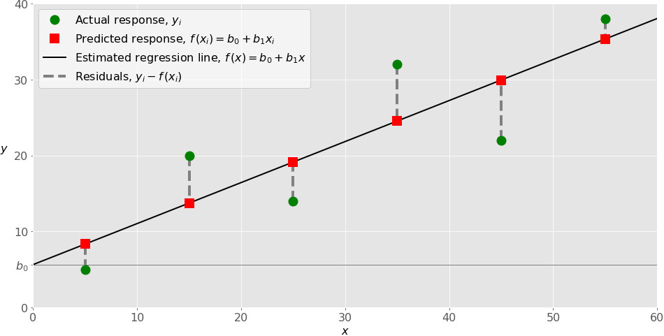
Реализация простой линейной регрессии начинается с заданным набором пар (зелёные круги) входов-выходов (x-y). Эти пары – результаты наблюдений. Наблюдение, крайнее слева (зелёный круг) имеет на входе x = 5 и соответствующий выход (ответ) y = 5. Следующее наблюдение имеет x = 15 и y = 20, и так далее.
Оценочная функция регрессии (чёрная линия) выражается уравнением f(x) = b₀ + b₁x. Нужно рассчитать оптимальные значения спрогнозированных весов b₀ и b₁ для минимизации SSR и определить оценочную функцию регрессии. Величина b₀, также называемая отрезком, показывает точку, где расчётная линия регрессии пересекает ось y. Это значение расчётного ответа f(x) для x = 0. Величина b₁ определяет наклон расчетной линии регрессии.
Предсказанные ответы (красные квадраты) – точки линии регрессии, соответствующие входным значениям. Для входа x = 5 предсказанный ответ равен f(5) = 8.33 (представленный крайним левыми квадратом).
Остатки (вертикальные пунктирные серые линии) могут быть вычислены как yᵢ − f(xᵢ) = yᵢ − b₀ − b₁xᵢ для i = 1, …, n. Они представляют собой расстояния между зелёными и красными пунктами. При реализации линейной регрессии вы минимизируете эти расстояния и делаете красные квадраты как можно ближе к предопределённым зелёным кругам.
Пришло время реализовать линейную регрессию в Python. Всё, что вам нужно, – подходящие пакеты, функции и классы.
Пакеты Python для линейной регрессии
NumPy – фундаментальный научный пакет для быстрых операций над одномерными и многомерными массивами. Он облегчает математическую рутину и, конечно, находится в open-source.
Незнакомы с NumPy? Начните с официального гайда.
Пакет scikit-learn – это библиотека, широко используемая в машинном обучении. Она предоставляет значения для данных предварительной обработки, уменьшает размерность, реализует регрессию, классификацию, кластеризацию и т. д. Находится в open-source, как и NumPy.
Начните знакомство с линейными моделями и работой пакета на сайте scikit-learn.
Простая линейная регрессия со scikit-learn
Начнём с простейшего случая линейной регрессии.
Следуйте пяти шагам реализации линейной регрессии:
- Импортируйте необходимые пакеты и классы.
- Предоставьте данные для работы и преобразования.
- Создайте модель регрессии и приспособьте к существующим данным.
- Проверьте результаты совмещения и удовлетворительность модели.
- Примените модель для прогнозов.
Это общие шаги для большинства подходов и реализаций регрессии.
Шаг 1: Импортируйте пакеты и классы
Первым шагом импортируем пакет NumPy и класс LinearRegressionиз sklearn.linear_model:
import numpy as np
from sklearn.linear_model import LinearRegression
Теперь у вас есть весь функционал для реализации линейной регрессии.
Фундаментальный тип данных NumPy – это тип массива numpy.ndarray. Далее под массивом подразумеваются все экземпляры типа numpy.ndarray.
Класс sklearn.linear_model.LinearRegression используем для линейной регрессии и прогнозов.
Шаг 2 : Предоставьте данные
Вторым шагом определите данные, с которыми предстоит работать. Входы (регрессоры, x) и выход (предиктор, y) должны быть массивами (экземпляры класса numpy.ndarray) или похожими объектами. Вот простейший способ предоставления данных регрессии:
x = np.array([5, 15, 25, 35, 45, 55]).reshape((-1, 1))
y = np.array([5, 20, 14, 32, 22, 38])
Теперь у вас два массива: вход x и выход y. Вам нужно вызвать .reshape()на x, потому что этот массив должен быть двумерным или более точным – иметь одну колонку и необходимое количество рядов. Это как раз то, что определяет аргумент (-1, 1).
Вот как x и y выглядят теперь:
>>> print(x)
[[ 5]
 [15]
 [25]
 [35]
 [45]
 [55]]
>>> print(y)
[ 5 20 14 32 22 38]
Шаг 3: Создайте модель
На этом шаге создайте и приспособьте модель линейной регрессии к существующим данным.
Давайте сделаем экземпляр класса LinearRegression, который представит модель регрессии:
model = LinearRegression()
Эта операция создаёт переменную model в качестве экземпляра LinearRegression. Вы можете предоставить несколько опциональных параметров классу LinearRegression:
- fit_intercept – логический (
Trueпо умолчанию) параметр, который решает, вычислять отрезок b₀ (True) или рассматривать его как равный нулю (False). - normalize – логический (
Falseпо умолчанию) параметр, который решает, нормализовать входные переменные (True) или нет (False). - copy_X – логический (
Trueпо умолчанию) параметр, который решает, копировать (True) или перезаписывать входные переменные (False). - n_jobs – целое или
None(по умолчанию), представляющее количество процессов, задействованных в параллельных вычислениях.Noneозначает отсутствие процессов, при -1 используются все доступные процессоры.
Наш пример использует состояния параметров по умолчанию.
Пришло время задействовать model. Сначала вызовите .fit() на model:
model.fit(x, y)
С помощью .fit() вычисляются оптимальные значение весов b₀ и b₁, используя существующие вход и выход (x и y) в качестве аргументов. Другими словами, .fit() совмещает модель. Она возвращает self — переменную model. Поэтому можно заменить две последние операции на:
model = LinearRegression().fit(x, y)
Эта операция короче и делает то же, что и две предыдущие.
Шаг 4: Получите результаты
После совмещения модели нужно убедиться в удовлетворительности результатов для интерпретации.
Вы можете получить определения (R²) с помощью .score(), вызванной на model:
>>> r_sq = model.score(x, y)
>>> print('coefficient of determination:', r_sq)
coefficient of determination: 0.715875613747954
.score() принимает в качестве аргументов предсказатель x и регрессор y, и возвращает значение R².
model содержит атрибуты .intercept_, который представляет собой коэффициент, и b₀ с .coef_, которые представляют b₁:
>>> print('intercept:', model.intercept_)
intercept: 5.633333333333329
>>> print('slope:', model.coef_)
slope: [0.54]
Код выше показывает, как получить b₀ и b₁. Заметьте, что .intercept_ – это скаляр, в то время как .coef_ – массив.
Примерное значение b₀ = 5.63 показывает, что ваша модель предсказывает ответ 5.63 при x, равном нулю. Равенство b₁ = 0.54 означает, что предсказанный ответ возрастает до 0.54 при x, увеличенным на единицу.
Заметьте, что вы можете предоставить y как двумерный массив. Тогда результаты не будут отличаться:
>>> new_model = LinearRegression().fit(x, y.reshape((-1, 1)))
>>> print('intercept:', new_model.intercept_)
intercept: [5.63333333]
>>> print('slope:', new_model.coef_)
slope: [[0.54]]
Как вы видите, пример похож на предыдущий, но в данном случае .intercept_ – одномерный массив с единственным элементом b₀, и .coef_ – двумерный массив с единственным элементом b₁.
Шаг 5: Предскажите ответ
Когда вас устроит ваша модель, вы можете использовать её для прогнозов с текущими или другими данными.
Получите предсказанный ответ, используя .predict():
>>> y_pred = model.predict(x)
>>> print('predicted response:', y_pred, sep='n')
predicted response:
[ 8.33333333 13.73333333 19.13333333 24.53333333 29.93333333 35.33333333]
Применяя .predict(), вы передаёте регрессор в качестве аргумента и получаете соответствующий предсказанный ответ.
Вот почти идентичный способ предсказать ответ:
>>> y_pred = model.intercept_ + model.coef_ * x
>>> print('predicted response:', y_pred, sep='n')
predicted response:
[[ 8.33333333]
 [13.73333333]
 [19.13333333]
 [24.53333333]
 [29.93333333]
 [35.33333333]]
В этом случае вы умножаете каждый элемент массива x с помощью model.coef_ и добавляете model.intercept_ в ваш продукт.
Вывод отличается от предыдущего примера количеством измерений. Теперь предсказанный ответ – это двумерный массив, в отличии от предыдущего случая, в котором он одномерный.
Измените количество измерений x до одного, и увидите одинаковый результат. Для этого замените x на x.reshape(-1), x.flatten() или x.ravel() при умножении с помощью model.coef_.
На практике модель регрессии часто используется для прогнозов. Это значит, что вы можете использовать приспособленные модели для вычисления выходов на базе других, новых входов:
>>> x_new = np.arange(5).reshape((-1, 1))
>>> print(x_new)
[[0]
 [1]
 [2]
 [3]
 [4]]
>>> y_new = model.predict(x_new)
>>> print(y_new)
[5.63333333 6.17333333 6.71333333 7.25333333 7.79333333]
Здесь .predict() применяется на новом регрессоре x_new и приводит к ответу y_new. Этот пример удобно использует arange() из NumPy для генерации массива с элементами от 0 (включительно) до 5 (исключительно) – 0, 1, 2, 3, и 4.
О LinearRegression вы узнаете больше из официальной документации.
Теперь у вас есть своя модель линейной регрессии!
Источник
Нравится Data Science? Другие материалы по теме:
- 6 советов, которые спасут специалиста Data Science
- Как изучать Data Science в 2019: ответы на частые вопросы
- Схема успешного развития data-scientist специалиста в 2019 году
Перевод
Ссылка на автора

Введение
Эта статья пытается быть справочной информацией, которая вам нужна, когда дело доходит до понимания и выполнения линейной регрессии. Хотя алгоритм прост, лишь немногие действительно понимают основные принципы.
Во-первых, мы углубимся в теорию линейной регрессии, чтобы понять ее внутреннюю работу. Затем мы реализуем алгоритм на Python для моделирования бизнес-задачи.
Я надеюсь, что эта статья найдет свой путь в ваши закладки! А пока давайте к этому!
Теория
Линейная регрессия, вероятно, является самым простым подходом для статистического обучения. Это хорошая отправная точка для более продвинутых подходов, и фактически многие причудливые статистические методы обучения можно рассматривать как расширение линейной регрессии. Следовательно, понимание этой простой модели создаст хорошую базу, прежде чем перейти к более сложным подходам.
Линейная регрессия очень хороша, чтобы ответить на следующие вопросы:
- Есть ли связь между 2 переменными?
- Насколько прочны отношения?
- Какая переменная вносит наибольший вклад?
- Насколько точно мы можем оценить влияние каждой переменной?
- Насколько точно мы можем предсказать цель?
- Являются ли отношения линейными? (Дух)
- Есть ли эффект взаимодействия?
Оценка коэффициентов
Предположим, у нас есть только одна переменная и одна цель. Тогда линейная регрессия выражается как:

В приведенном выше уравнениибетыявляются коэффициентами. Эти коэффициенты — то, что нам нужно, чтобы делать прогнозы с нашей моделью.
Итак, как мы можем найти эти параметры?
Чтобы найти параметры, нам нужно минимизироватьнаименьших квадратовилисумма квадратов ошибок, Конечно, линейная модель не идеальна, и она не будет точно предсказывать все данные, а это означает, что существует разница между фактическим значением и прогнозом. Ошибка легко вычисляется с помощью:

Но почему ошибки возводятся в квадрат?
Мы возводим в квадрат ошибку, потому что прогноз может быть выше или ниже истинного значения, что приводит к отрицательной или положительной разнице соответственно. Если бы мы не возводили в квадрат ошибки, сумма ошибок могла бы уменьшиться из-за отрицательных различий, а не потому, что модель хорошо подходит.
Кроме того, возведение в квадрат ошибок учитывает большие различия, поэтому минимизация квадратов ошибок «гарантирует» лучшую модель.
Давайте посмотрим на график, чтобы лучше понять.

На приведенном выше графике красные точки — это истинные данные, а синяя линия — линейная модель. Серые линии иллюстрируют ошибки между предсказанными и истинными значениями. Таким образом, синяя линия — это та, которая минимизирует сумму квадратов длины серых линий.
После некоторой математики, которая является слишком тяжелой для этой статьи, вы можете наконец оценить коэффициенты с помощью следующих уравнений:


гдех бара такжеу барпредставляют собой среднее.
Оцените актуальность коэффициентов
Теперь, когда у вас есть коэффициенты, как вы можете определить, актуальны ли они для прогнозирования вашей цели?
Лучший способ — найтир-значение.р-значениеиспользуется для количественной оценки статистической значимости; это позволяет определить, следует ли отклонить нулевую гипотезу или нет.
Нулевая гипотеза?
Для любой задачи моделирования гипотеза состоит в том, чтоесть некоторая корреляциямежду функциями и целью. Таким образом, нулевая гипотеза противоположна:нет корреляциимежду функциями и целью.
Итак, нахождениер-значениедля каждого коэффициента будет указано, является ли переменная статистически значимой для прогнозирования цели. Как правило, еслир-значениеявляетсяменее чем 0,05: между переменной и целью существует тесная связь.
Оцените точность модели
Вы обнаружили, что ваша переменная была статистически значимой, найдя еер-значение, Большой!
Теперь, как узнать, хороша ли ваша линейная модель?
Чтобы оценить это, мы обычно используем RSE (остаточная стандартная ошибка) и статистику R².


Первая метрика ошибки проста для понимания: чем меньше остаточных ошибок, тем лучше модель соответствует данным (в этом случае, чем ближе данные к линейной зависимости).
Что касается метрики R², он измеряетдоля изменчивости в цели, которая может быть объяснена с помощью функции X, Следовательно, при условии линейного отношения, если признак X может объяснить (предсказать) цель, тогда пропорция высока, и значение R² будет близко к 1. Если противоположное верно, значение R² будет тогда ближе к 0.
Теория множественной линейной регрессии
В реальных ситуациях никогда не будет единственной функции, чтобы предсказать цель Итак, выполняем ли мы линейную регрессию по одному объекту за раз? Конечно нет. Мы просто выполняем множественную линейную регрессию.
Уравнение очень похоже на простую линейную регрессию; просто добавьте количество предикторов и соответствующие им коэффициенты:

Оцените актуальность предиктора
Ранее в простой линейной регрессии мы оценивали релевантность функции, находя еер-значение,
В случае множественной линейной регрессии мы используем другую метрику: F-статистику.

Здесь F-статистика рассчитывается для всей модели, тогда какр-значениеспецифичен для каждого предиктора. Если существует сильная связь, то F будет намного больше 1. В противном случае она будет приблизительно равна 1.
Какбольшечем 1достаточно большой?
Это сложно ответить. Обычно, если имеется большое количество точек данных, F может быть немного больше 1 и предполагать тесную связь. Для небольших наборов данных значение F должно быть намного больше 1, чтобы предполагать тесную связь.
Почему мы не можем использоватьр-значениев этом случае?
Поскольку мы подгоняем много предикторов, нам нужно рассмотреть случай, когда есть много функций (пбольшой). При очень большом количестве предикторов всегда будет около 5%, у которых, случайнор-значениечетноехотя они не являются статистически значимыми.Поэтому мы используем F-статистику, чтобы не рассматривать неважные предикторы как значимые предикторы.
Оцените точность модели
Как и в простой линейной регрессии, R² может использоваться для множественной линейной регрессии. Однако знайте, что добавление большего количества предикторов всегда будет увеличивать значение R², потому что модель обязательно будет лучше соответствовать обучающим данным.
Тем не менее, это не означает, что он будет хорошо работать с тестовыми данными (делая прогнозы для неизвестных точек данных).
Добавление взаимодействия
Наличие нескольких предикторов в линейной модели означает, что некоторые предикторы могут влиять на другие предикторы.
Например, вы хотите предсказать зарплату человека, зная его возраст и количество лет, проведенных в школе. Конечно, чем старше человек, тем больше времени он мог бы проводить в школе. Итак, как мы моделируем этот эффект взаимодействия?
Рассмотрим этот очень простой пример с двумя предикторами:

Как видите, мы просто умножаем оба предиктора вместе и связываем новый коэффициент. Упрощая формулу, мы теперь видим, что на коэффициент влияет значение другого признака.
Как правило, если мы включаем модель взаимодействия, мы должны включать индивидуальный эффект объекта, даже если егор-значениенезначительный. Это известно какиерархический принцип, Это объясняется тем, что если два предиктора взаимодействуют, то включение их индивидуального вклада окажет небольшое влияние на модель.
Хорошо! Теперь, когда мы знаем, как это работает, давайте заставим это работать! Мы будем работать как с простой, так и с множественной линейной регрессией в Python, и я покажу, как оценивать качество параметров и общую модель в обеих ситуациях.
Вы можете получить код и данные Вот,
Я настоятельно рекомендую вам следовать и воссоздать шаги в своем собственном блокноте Jupyter, чтобы в полной мере воспользоваться этим руководством.
Давайте доберемся до этого!
Введение
Набор данных содержит информацию о деньгах, потраченных на рекламу, и их продажах. Деньги были потрачены на рекламу на телевидении, радио и в газетах.
Цель состоит в том, чтобы использовать линейную регрессию, чтобы понять, как расходы на рекламу влияют на продажи.
Импорт библиотек
Преимущество работы с Python заключается в том, что у нас есть доступ ко многим библиотекам, которые позволяют нам быстро читать данные, наносить на график данные и выполнять линейную регрессию.
Мне нравится импортировать все необходимые библиотеки поверх ноутбука, чтобы все было организовано. Импортируйте следующее:
import pandas as pd
import numpy as npimport matplotlib.pyplot as pltfrom sklearn.linear_model import LinearRegression
from sklearn.metrics import r2_scoreimport statsmodels.api as sm
Читать данные
Предполагая, что вы загрузили набор данных, поместите его вdataкаталог в папке вашего проекта. Затем прочитайте данные так:
data = pd.read_csv("data/Advertising.csv")
Чтобы увидеть, как выглядят данные, мы делаем следующее:
data.head()
И вы должны увидеть это:

Как видите, столбецUnnamed: 0избыточно Следовательно, мы удалим это.
data.drop(['Unnamed: 0'], axis=1)
Хорошо, наши данные чисты и готовы к линейной регрессии!
Простая линейная регрессия
моделирование
Для простой линейной регрессии, давайте рассмотрим только влияние телевизионной рекламы на продажи. Прежде чем перейти непосредственно к моделированию, давайте посмотрим, как выглядят данные.
Мы используемmatplotlib, популярная библиотека для построения графиков на Python
plt.figure(figsize=(16, 8))
plt.scatter(
    data['TV'],
    data['sales'],
    c='black'
)
plt.xlabel("Money spent on TV ads ($)")
plt.ylabel("Sales ($)")
plt.show()
Запустите эту ячейку кода, и вы должны увидеть этот график:

Как видите, существует четкая взаимосвязь между суммой, потраченной на телевизионную рекламу, и продажами.
Давайте посмотрим, как мы можем сгенерировать линейное приближение этих данных.
X = data['TV'].values.reshape(-1,1)
y = data['sales'].values.reshape(-1,1)reg = LinearRegression()
reg.fit(X, y)print("The linear model is: Y = {:.5} + {:.5}X".format(reg.intercept_[0], reg.coef_[0][0]))
Это оно?
Да! Это так просто, чтобы подогнать прямую линию к набору данных и увидеть параметры уравнения. В этом случае мы имеем

Давайте представим, как линия соответствует данным.
predictions = reg.predict(X)plt.figure(figsize=(16, 8))
plt.scatter(
    data['TV'],
    data['sales'],
    c='black'
)
plt.plot(
    data['TV'],
    predictions,
    c='blue',
    linewidth=2
)
plt.xlabel("Money spent on TV ads ($)")
plt.ylabel("Sales ($)")
plt.show()
И теперь вы видите:

Из приведенного выше графика видно, что простая линейная регрессия может объяснить общее влияние суммы, потраченной на телевизионную рекламу и продажи.
Оценка актуальности модели
Теперь, если вы помните из этого после, чтобы увидеть, является ли модель хорошей, нам нужно посмотреть на значение R² ир-значениеот каждого коэффициента.
Вот как мы это делаем:
X = data['TV']
y = data['sales']X2 = sm.add_constant(X)
est = sm.OLS(y, X2)
est2 = est.fit()
print(est2.summary())
Что дает вам этот прекрасный вывод:

Глядя на оба коэффициента, мы имеемр-значениеэто очень мало (хотя, вероятно, это не совсем 0). Это означает, что существует сильная корреляция между этими коэффициентами и целью (продажи).
Затем, глядя на значение R², мы получаем 0,612. Следовательно,около 60% изменчивости продаж объясняется суммой, потраченной на телевизионную рекламу, Это нормально, но точно не лучшее, что мы можем точно предсказать продажи. Конечно, расходы на рекламу в газетах и на радио должны оказывать определенное влияние на продажи.
Посмотрим, будет ли лучше работать множественная линейная регрессия.
Множественная линейная регрессия
моделирование
Как и для простой линейной регрессии, мы определим наши функции и целевую переменную и используемscikit учитьсябиблиотека для выполнения линейной регрессии.
Xs = data.drop(['sales', 'Unnamed: 0'], axis=1)
y = data['sales'].reshape(-1,1)reg = LinearRegression()
reg.fit(Xs, y)print("The linear model is: Y = {:.5} + {:.5}*TV + {:.5}*radio + {:.5}*newspaper".format(reg.intercept_[0], reg.coef_[0][0], reg.coef_[0][1], reg.coef_[0][2]))
Больше ничего! Из этой ячейки кода мы получаем следующее уравнение:

Конечно, мы не можем визуализировать влияние всех трех сред на продажи, так как оно имеет четыре измерения.
Обратите внимание, что коэффициент для газеты является отрицательным, но также довольно небольшим. Это относится к нашей модели? Давайте посмотрим, рассчитав F-статистику, значение R² ир-значениеза каждый коэффициент.
Оценка актуальности модели
Как и следовало ожидать, процедура здесь очень похожа на то, что мы делали в простой линейной регрессии.
X = np.column_stack((data['TV'], data['radio'], data['newspaper']))
y = data['sales']X2 = sm.add_constant(X)
est = sm.OLS(y, X2)
est2 = est.fit()
print(est2.summary())
И вы получите следующее:

Как вы можете видеть, R² намного выше, чем у простой линейной регрессии, со значением0,897!
Кроме того, F-статистика570,3, Это намного больше, чем 1, и поскольку наш набор данных достаточно мал (всего 200 точек),демонстрирует тесную связь между расходами на рекламу и продажами,
Наконец, поскольку у нас есть только три предиктора, мы можем рассмотреть ихр-значениеопределить, имеют ли они отношение к модели или нет. Конечно, вы заметили, что третий коэффициент (для газеты) имеет большойр-значение, Поэтому рекламные расходы на газетуне является статистически значимым, Удаление этого предиктора немного уменьшит значение R², но мы могли бы сделать более точные прогнозы.
Вы качаетесь 🤘. Поздравляю с завершением, теперь вы мастер линейной регрессии!
Как упоминалось выше, это может быть не самый эффективный алгоритм, но он важен для понимания линейной регрессии, поскольку он формирует основу более сложных статистических подходов к обучению.
Я надеюсь, что вы когда-нибудь вернетесь к этой статье.
Ура!
- class sklearn.linear_model.LinearRegression(*, fit_intercept=True, copy_X=True, n_jobs=None, positive=False)[source]
-
Ordinary least squares Linear Regression.
LinearRegression fits a linear model with coefficients w = (w1, …, wp)
to minimize the residual sum of squares between the observed targets in
the dataset, and the targets predicted by the linear approximation.- Parameters:
-
- fit_interceptbool, default=True
-
Whether to calculate the intercept for this model. If set
to False, no intercept will be used in calculations
(i.e. data is expected to be centered). - copy_Xbool, default=True
-
If True, X will be copied; else, it may be overwritten.
- n_jobsint, default=None
-
The number of jobs to use for the computation. This will only provide
speedup in case of sufficiently large problems, that is if firstly
n_targets > 1and secondlyXis sparse or ifpositiveis set
toTrue.Nonemeans 1 unless in a
joblib.parallel_backendcontext.-1means using all
processors. See Glossary for more details. - positivebool, default=False
-
When set to
True, forces the coefficients to be positive. This
option is only supported for dense arrays.New in version 0.24.
- Attributes:
-
- coef_array of shape (n_features, ) or (n_targets, n_features)
-
Estimated coefficients for the linear regression problem.
If multiple targets are passed during the fit (y 2D), this
is a 2D array of shape (n_targets, n_features), while if only
one target is passed, this is a 1D array of length n_features. - rank_int
-
Rank of matrix
X. Only available whenXis dense. - singular_array of shape (min(X, y),)
-
Singular values of
X. Only available whenXis dense. - intercept_float or array of shape (n_targets,)
-
Independent term in the linear model. Set to 0.0 if
fit_intercept = False. - n_features_in_int
-
Number of features seen during fit.
New in version 0.24.
- feature_names_in_ndarray of shape (
n_features_in_,) -
Names of features seen during fit. Defined only when
X
has feature names that are all strings.New in version 1.0.
See also
Ridge-
Ridge regression addresses some of the problems of Ordinary Least Squares by imposing a penalty on the size of the coefficients with l2 regularization.
Lasso-
The Lasso is a linear model that estimates sparse coefficients with l1 regularization.
ElasticNet-
Elastic-Net is a linear regression model trained with both l1 and l2 -norm regularization of the coefficients.
Notes
From the implementation point of view, this is just plain Ordinary
Least Squares (scipy.linalg.lstsq) or Non Negative Least Squares
(scipy.optimize.nnls) wrapped as a predictor object.Examples
>>> import numpy as np
>>> from sklearn.linear_model import LinearRegression
>>> X = np.array([[1, 1], [1, 2], [2, 2], [2, 3]])
>>> # y = 1 * x_0 + 2 * x_1 + 3
>>> y = np.dot(X, np.array([1, 2])) + 3
>>> reg = LinearRegression().fit(X, y)
>>> reg.score(X, y)
1.0
>>> reg.coef_
array([1., 2.])
>>> reg.intercept_
3.0...
>>> reg.predict(np.array([[3, 5]]))
array([16.])
Methods
fit(X, y[, sample_weight])Fit linear model.
get_params([deep])Get parameters for this estimator.
predict(X)Predict using the linear model.
score(X, y[, sample_weight])Return the coefficient of determination of the prediction.
set_params(**params)Set the parameters of this estimator.
- fit(X, y, sample_weight=None)[source]
-
Fit linear model.
- Parameters:
-
- X{array-like, sparse matrix} of shape (n_samples, n_features)
-
Training data.
- yarray-like of shape (n_samples,) or (n_samples, n_targets)
-
Target values. Will be cast to X’s dtype if necessary.
- sample_weightarray-like of shape (n_samples,), default=None
-
Individual weights for each sample.
New in version 0.17: parameter sample_weight support to LinearRegression.
- Returns:
-
- selfobject
-
Fitted Estimator.
- get_params(deep=True)[source]
-
Get parameters for this estimator.
- Parameters:
-
- deepbool, default=True
-
If True, will return the parameters for this estimator and
contained subobjects that are estimators.
- Returns:
-
- paramsdict
-
Parameter names mapped to their values.
- predict(X)[source]
-
Predict using the linear model.
- Parameters:
-
- Xarray-like or sparse matrix, shape (n_samples, n_features)
-
Samples.
- Returns:
-
- Carray, shape (n_samples,)
-
Returns predicted values.
- score(X, y, sample_weight=None)[source]
-
Return the coefficient of determination of the prediction.
The coefficient of determination (R^2) is defined as
((1 — frac{u}{v})), where (u) is the residual
sum of squares((y_true - y_pred)** 2).sum()and (v)
is the total sum of squares((y_true - y_true.mean()) ** 2).sum().
The best possible score is 1.0 and it can be negative (because the
model can be arbitrarily worse). A constant model that always predicts
the expected value ofy, disregarding the input features, would get
a (R^2) score of 0.0.- Parameters:
-
- Xarray-like of shape (n_samples, n_features)
-
Test samples. For some estimators this may be a precomputed
kernel matrix or a list of generic objects instead with shape
(n_samples, n_samples_fitted), wheren_samples_fitted
is the number of samples used in the fitting for the estimator. - yarray-like of shape (n_samples,) or (n_samples, n_outputs)
-
True values for
X. - sample_weightarray-like of shape (n_samples,), default=None
-
Sample weights.
- Returns:
-
- scorefloat
-
(R^2) of
self.predict(X)wrt.y.
Notes
The (R^2) score used when calling
scoreon a regressor uses
multioutput='uniform_average'from version 0.23 to keep consistent
with default value ofr2_score.
This influences thescoremethod of all the multioutput
regressors (except for
MultiOutputRegressor).
- set_params(**params)[source]
-
Set the parameters of this estimator.
The method works on simple estimators as well as on nested objects
(such asPipeline). The latter have
parameters of the form<component>__<parameter>so that it’s
possible to update each component of a nested object.- Parameters:
-
- **paramsdict
-
Estimator parameters.
- Returns:
-
- selfestimator instance
-
Estimator instance.
Examples using sklearn.linear_model.LinearRegression
If you had studied longer, would your overall scores get any better?
One way of answering this question is by having data on how long you studied for and what scores you got. We can then try to see if there is a pattern in that data, and if in that pattern, when you add to the hours, it also ends up adding to the scores percentage.
For instance, say you have an hour-score dataset, which contains entries such as 1.5h and 87.5% score. It could also contain 1.61h, 2.32h and 78%, 97% scores. The kind of data type that can have any intermediate value (or any level of ‘granularity’) is known as continuous data.
Another scenario is that you have an hour-score dataset which contains letter-based grades instead of number-based grades, such as A, B or C. Grades are clear values that can be isolated, since you can’t have an A.23, A+++++++++++ (and to infinity) or A * e^12. The kind of data type that cannot be partitioned or defined more granularly is known as discrete data.
Based on the modality (form) of your data — to figure out what score you’d get based on your study time — you’ll perform regression or classification.
Regression is performed on continuous data, while classification is performed on discrete data. Regression can be anything from predicting someone’s age, the house of a price, or value of any variable. Classification includes predicting what class something belongs to (such as whether a tumor is benign or malignant).
Note: Predicting house prices and whether a cancer is present is no small task, and both typically include non-linear relationships. Linear relationships are fairly simple to model, as you’ll see in a moment.
If you want to learn through real-world, example-led, practical projects, check out our «Hands-On House Price Prediction — Machine Learning in Python» and our research-grade «Breast Cancer Classification with Deep Learning — Keras and Tensorflow»!
For both regression and classification — we’ll use data to predict labels (umbrella-term for the target variables). Labels can be anything from «B» (class) for classification tasks to 123 (number) for regression tasks. Because we’re also supplying the labels — these are supervised learning algorithms.
In this beginner-oriented guide — we’ll be performing linear regression in Python, utilizing the Scikit-Learn library. We’ll go through an end-to-end machine learning pipeline. We’ll first load the data we’ll be learning from and visualizing it, at the same time performing Exploratory Data Analysis. Then, we’ll pre-process the data and build models to fit it (like a glove). This model is then evaluated, and if favorable, used to predict new values based on new input.
Note: You can download the notebook containing all of the code in this guide here.
Exploratory Data Analysis
Note: You can download the hour-score dataset here.
Let’s start with exploratory data analysis. You want to get to know your data first — this includes loading it in, visualizing features, exploring their relationships and making hypotheses based on your observations. The dataset is a CSV (comma-separated values) file, which contains the hours studied and the scores obtained based on those hours. We’ll load the data into a DataFrame using Pandas:
import pandas as pd
If you’re new to Pandas and
DataFrames, read our «Guide to Python with Pandas: DataFrame Tutorial with Examples»!
Let’s read the CSV file and package it into a DataFrame:
# Substitute the path_to_file content by the path to your student_scores.csv file
path_to_file = 'home/projects/datasets/student_scores.csv'
df = pd.read_csv(path_to_file)
Once the data is loaded in, let’s take a quick peek at the first 5 values using the head() method:
df.head()
This results in:
   Hours  Scores
0    2.5      21
1    5.1      47
2    3.2      27
3    8.5      75
4    3.5      30
We can also check the shape of our dataset via the shape property:
df.shape
Knowing the shape of your data is generally pretty crucial to being able to both analyze it and build models around it:
(25, 2)
We have 25 rows and 2 columns — that’s 25 entries containing a pair of an hour and a score. Our initial question was whether we’d score a higher score if we’d studied longer. In essence, we’re asking for the relationship between Hours and Scores. So, what’s the relationship between these variables? A great way to explore relationships between variables is through Scatterplots. We’ll plot the hours on the X-axis and scores on the Y-axis, and for each pair, a marker will be positioned based on their values:
df.plot.scatter(x='Hours', y='Scores', title='Scatterplot of hours and scores percentages');
If you’re new to Scatter Plots — read our «Matplotlib Scatter Plot — Tutorial and Examples»!
This results in:
As the hours increase, so do the scores. There’s a fairly high positive correlation here! Since the shape of the line the points are making appears to be straight — we say that there’s a positive linear correlation between the Hours and Scores variables. How correlated are they? The corr() method calculates and displays the correlations between numerical variables in a DataFrame:
print(df.corr())
           Hours    Scores
Hours   1.000000  0.976191
Scores  0.976191  1.000000
In this table, Hours and Hours have a 1.0 (100%) correlation, just as Scores have a 100% correlation to Scores, naturally. Any variable will have a 1:1 mapping with itself! However, the correlation between Scores and Hours is 0.97. Anything above 0.8 is considered to be a strong positive correlation.
If you’d like to read more about correlation between linear variables in detail, as well as different correlation coefficients, read our «Calculating Pearson Correlation Coefficient in Python with Numpy»!
Having a high linear correlation means that we’ll generally be able to tell the value of one feature, based on the other. Even without calculation, you can tell that if someone studies for 5 hours, they’ll get around 50% as their score. Since this relationship is really strong — we’ll be able to build a simple yet accurate linear regression algorithm to predict the score based on the study time, on this dataset.
When we have a linear relationship between two variables, we will be looking at a line. When there is a linear relationship between three, four, five (or more) variables, we will be looking at an intersecction of planes. In every case, this kind of quality is defined in algebra as linearity.
Pandas also ships with a great helper method for statistical summaries, and we can describe() the dataset to get an idea of the mean, maximum, minimum, etc. values of our columns:
print(df.describe())
           Hours     Scores
count  25.000000  25.000000
mean    5.012000  51.480000
std     2.525094  25.286887
min     1.100000  17.000000
25%     2.700000  30.000000
50%     4.800000  47.000000
75%     7.400000  75.000000
max     9.200000  95.000000
Linear Regression Theory
Our variables express a linear relationship. We can intuitively guesstimate the score percentage based on the number of hours studied. However, can we define a more formal way to do this? We could trace a line in between our points and read the value of «Score» if we trace a vertical line from a given value of «Hours»:
The equation that describes any straight line is:
$$
y = a*x+b
$$
In this equation, y represents the score percentage, x represent the hours studied. b is where the line starts at the Y-axis, also called the Y-axis intercept and a defines if the line is going to be more towards the upper or lower part of the graph (the angle of the line), so it is called the slope of the line.
By adjusting the slope and intercept of the line, we can move it in any direction. Thus — by figuring out the slope and intercept values, we can adjust a line to fit our data!
That’s it! That’s the heart of linear regression and an algorithm really only figures out the values of the slope and intercept. It uses the values of x and y that we already have and varies the values of a and b. By doing that, it fits multiple lines to the data points and returns the line that is closer to all the data points, or the best fitting line. By modelling that linear relationship, our regression algorithm is also called a model. In this process, when we try to determine, or predict the percentage based on the hours, it means that our y variable depends on the values of our x variable.
Note: In Statistics, it is customary to call y the dependent variable, and x the independent variable. In Computer Science, y is usually called target, label, and x feature, or attribute. You will see that the names interchange, keep in mind that there is usually a variable that we want to predict and another used to find it’s value. It’s also a convention to use capitalized X instead of lower case, in both Statistics and CS.
Linear Regression with Python’s Scikit-learn
With the theory under our belts — let’s get to implementing a Linear Regression algorithm with Python and the Scikit-Learn library! We’ll start with a simpler linear regression and then expand onto multiple linear regression with a new dataset.
Data Preprocessing
In the the previous section, we have already imported Pandas, loaded our file into a DataFrame and plotted a graph to see if there was an indication of a linear relationship. Now, we can divide our data in two arrays — one for the dependent feature and one for the independent, or target feature. Since we want to predict the score percentage depending on the hours studied, our y will be the «Score» column and our X will the «Hours» column.
To separate the target and features, we can attribute the dataframe column values to our y and X variables:
y = df['Scores'].values.reshape(-1, 1)
X = df['Hours'].values.reshape(-1, 1)
Note: df['Column_Name'] returns a pandas Series. Some libraries can work on a Series just as they would on a NumPy array, but not all libraries have this awareness. In some cases, you’ll want to extract the underlying NumPy array that describes your data. This is easily done via the values field of the Series.
Scikit-Learn’s linear regression model expects a 2D input, and we’re really offering a 1D array if we just extract the values:
print(df['Hours'].values) # [2.5 5.1 3.2 8.5 3.5 1.5 9.2 ... ]
print(df['Hours'].values.shape) # (25,)
It’s expect a 2D input because the LinearRegression() class (more on it later) expects entries that may contain more than a single value (but can also be a single value). In either case — it has to be a 2D array, where each element (hour) is actually a 1-element array:
print(X.shape) # (25, 1)
print(X)      # [[2.5] [5.1]  [3.2] ... ]
We could already feed our X and y data directly to our linear regression model, but if we use all of our data at once, how can we know if our results are any good? Just like in learning, what we will do, is use a part of the data to train our model and another part of it, to test it.
If you’d like to read more about the rules of thumb, importance of splitting sets, validation sets and the
train_test_split()helper method, read our detailed guide on «Scikit-Learn’s train_test_split() — Training, Testing and Validation Sets»!
This is easily achieved through the helper train_test_split() method, which accepts our X and y arrays (also works on DataFrames and splits a single DataFrame into training and testing sets), and a test_size. The test_size is the percentage of the overall data we’ll be using for testing:
from sklearn.model_selection import train_test_split
X_train, X_test, y_train, y_test = train_test_split(X, y, test_size = 0.2)
The method randomly takes samples respecting the percentage we’ve defined, but respects the X-y pairs, lest the sampling would totally mix up the relationship. Some common train-test splits are 80/20 and 70/30.
Since the sampling process is inherently random, we will always have different results when running the method. To be able to have the same results, or reproducible results, we can define a constant called SEED that has the value of the meaning of life (42):
SEED = 42
Note: The seed can be any integer, and is used as the seed for the random sampler. The seed is usually random, netting different results. However, if you set it manually, the sampler will return the same results. It’s convention to use 42 as the seed as a reference to the popular novel series «The Hitchhiker’s Guide to the Galaxy».
We can then pass that SEEDto the random_state parameter of our train_test_split method:
X_train, X_test, y_train, y_test = train_test_split(X, y, test_size = 0.2, random_state = SEED)
Now, if you print your X_train array — you’ll find the study hours, and y_train contains the score percentages:
print(X_train) # [[2.7] [3.3] [5.1] [3.8] ... ]
print(y_train) # [[25] [42] [47] [35] ... ]
Training a Linear Regression Model
We have our train and test sets ready. Scikit-Learn has a plethora of model types we can easily import and train, LinearRegression being one of them:
from sklearn.linear_model import LinearRegression
regressor = LinearRegression()
Now, we need to fit the line to our data, we will do that by using the .fit() method along with our X_train and y_train data:
regressor.fit(X_train, y_train)
If no errors are thrown — the regressor found the best fitting line! The line is defined by our features and the intercept/slope. In fact, we can inspect the intercept and slope by printing the regressor.intecept_ and regressor.coef_ attributes, respectively:
print(regressor.intercept_)
2.82689235
For retrieving the slope (which is also the coefficient of x):
print(regressor.coef_)
The result should be:
[9.68207815]
This can quite literally be plugged in into our formula from before:
$$
score = 9.68207815*hours+2.82689235
$$
Let’s check real quick whether this aligns with our guesstimation:
h
o
u
r
s
=
5
s
c
o
r
e
=
9.68207815
∗
h
o
u
r
s
+
2.82689235
s
c
o
r
e
=
51.2672831
With 5 hours of study, you can expect around 51% as a score! Another way to interpret the intercept value is — if a student studies one hour more than they previously studied for an exam, they can expect to have an increase of 9.68% considering the score percentage that they had previously achieved.
In other words, the slope value shows what happens to the dependent variable whenever there is an increase (or decrease) of one unit of the independent variable.
Making Predictions
To avoid running calculations ourselves, we could write our own formula that calculates the value:
def calc(slope, intercept, hours):
    return slope*hours+intercept

score = calc(regressor.coef_, regressor.intercept_, 9.5)
print(score) # [[94.80663482]]
However — a much handier way to predict new values using our model is to call on the predict() function:
# Passing 9.5 in double brackets to have a 2 dimensional array
score = regressor.predict([[9.5]])
print(score) # 94.80663482
Our result is 94.80663482, or approximately 95%. Now we have a score percentage estimate for each and every hours we can think of. But can we trust those estimates? In the answer to that question is the reason why we split the data into train and test in the first place. Now we can predict using our test data and compare the predicted with our actual results — the ground truth results.
To make predictions on the test data, we pass the X_test values to the predict() method. We can assign the results to the variable y_pred:
y_pred = regressor.predict(X_test)
The y_pred variable now contains all the predicted values for the input values in the X_test. We can now compare the actual output values for X_test with the predicted values, by arranging them side by side in a dataframe structure:
df_preds = pd.DataFrame({'Actual': y_test.squeeze(), 'Predicted': y_pred.squeeze()})
print(df_preds
The output looks like this:
   Actual  Predicted
0      81  83.188141
1      30  27.032088
2      21  27.032088
3      76  69.633232
4      62  59.951153
Though our model seems not to be very precise, the predicted percentages are close to the actual ones. Let’s quantify the difference between the actual and predicted values to gain an objective view of how it’s actually performing.
Evaluating the Model
After looking at the data, seeing a linear relationship, training and testing our model, we can understand how well it predicts by using some metrics. For regression models, three evaluation metrics are mainly used:
- Mean Absolute Error (MAE): When we subtract the predicted values from the actual values, obtaining the errors, sum the absolute values of those errors and get their mean. This metric gives a notion of the overall error for each prediction of the model, the smaller (closer to 0) the better.
$$
mae = (frac{1}{n})sum_{i=1}^{n}left | Actual — Predicted right |
$$
Note: You may also encounter the y and ŷ notation in the equations. The y refers to the actual values and the ŷ to the predicted values.
- Mean Squared Error (MSE): It is similar to the MAE metric, but it squares the absolute values of the errors. Also, as with MAE, the smaller, or closer to 0, the better. The MSE value is squared so as to make large errors even larger. One thing to pay close attention to, it that it is usually a hard metric to interpret due to the size of its values and of the fact that they aren’t in the same scale of the data.
$$
mse = sum_{i=1}^{D}(Actual — Predicted)^2
$$
- Root Mean Squared Error (RMSE): Tries to solve the interpretation problem raised with the MSE by getting the square root of its final value, so as to scale it back to the same units of the data. It is easier to interpret and good when we need to display or show the actual value of the data with the error. It shows how much the data may vary, so, if we have an RMSE of 4.35, our model can make an error either because it added 4.35 to the actual value, or needed 4.35 to get to the actual value. The closer to 0, the better as well.
$$
rmse = sqrt{ sum_{i=1}^{D}(Actual — Predicted)^2}
$$
We can use any of those three metrics to compare models (if we need to choose one). We can also compare the same regression model with different argument values or with different data and then consider the evaluation metrics. This is known as hyperparameter tuning — tuning the hyperparameters that influence a learning algorithm and observing the results.
When choosing between models, the ones with the smallest errors, usually perform better. When monitoring models, if the metrics got worse, then a previous version of the model was better, or there was some significant alteration in the data for the model to perform worse than it was performing.
Luckily, we don’t have to do any of the metrics calculations manually. The Scikit-Learn package already comes with functions that can be used to find out the values of these metrics for us. Let’s find the values for these metrics using our test data. First, we will import the necessary modules for calculating the MAE and MSE errors. Respectively, the mean_absolute_error and mean_squared_error:
from sklearn.metrics import mean_absolute_error, mean_squared_error
Now, we can calculate the MAE and MSE by passing the y_test (actual) and y_pred (predicted) to the methods. The RMSE can be calculated by taking the square root of the MSE, to to that, we will use NumPy’s sqrt() method:
import numpy as np
For the metrics calculations:
mae = mean_absolute_error(y_test, y_pred)
mse = mean_squared_error(y_test, y_pred)
rmse = np.sqrt(mse)
We will also print the metrics results using the f string and the 2 digit precision after the comma with :.2f:
print(f'Mean absolute error: {mae:.2f}')
print(f'Mean squared error: {mse:.2f}')
print(f'Root mean squared error: {rmse:.2f}')
The results of the metrics will look like this:
Mean absolute error: 3.92
Mean squared error: 18.94
Root mean squared error: 4.35
All of our errors are low — and we’re missing the actual value by 4.35 at most (lower or higher), which is a pretty small range considering the data we have.
Multiple Linear Regression
Until this point, we have predicted a value with linear regression using only one variable. There is a different scenario that we can consider, where we can predict using many variables instead of one, and this is also a much more common scenario in real life, where many things can affect some result.
For instance, if we want to predict the gas consumption in US states, it would be limiting to use only one variable, for instance, gas taxes, to do it, since more than just gas taxes affects consumption. There are more things involved in the gas consumption than only gas taxes, such as the per capita income of the people in a certain area, the extension of paved highways, the proportion of the population that has a driver’s license, and many other factors. Some factors affect the consumption more than others — and here’s where correlation coefficients really help!
In a case like this, when it makes sense to use multiple variables, linear regression becomes a multiple linear regression.
Note: Another nomenclature for the linear regression with one independent variable is univariate linear regression. And for the multiple linear regression, with many independent variables, is multivariate linear regression.
Usually, real world data, by having much more variables with greater values range, or more variability, and also complex relationships between variables — will involve multiple linear regression instead of a simple linear regression.
That is to say, on a day-to-day basis, if there is linearity in your data, you will probably be applying a multiple linear regression to your data.
Exploratory Data Analysis
To get a practical sense of multiple linear regression, let’s keep working with our gas consumption example, and use a dataset that has gas consumption data on 48 US States.
Note: You can download the gas consumption dataset on Kaggle. You can learn more about the details on the dataset here.
Following what we did with the linear regression, we will also want to know our data before applying multiple linear regression. First, we can import the data with pandas read_csv() method:
path_to_file = 'home/projects/datasets/petrol_consumption.csv'
df = pd.read_csv(path_to_file)
We can now take a look at the first five rows with df.head():
df.head()
This results in:
	Petrol_tax	Average_income	Paved_Highways	Population_Driver_licence(%)  Petrol_Consumption
0	9.0			3571			1976			0.525						  541
1	9.0			4092			1250			0.572						  524
2	9.0			3865			1586			0.580						  561
3	7.5			4870			2351			0.529						  414
4	8.0			4399			431				0.544						  410
We can see the how many rows and columns our data has with shape:
df.shape
Check out our hands-on, practical guide to learning Git, with best-practices, industry-accepted standards, and included cheat sheet. Stop Googling Git commands and actually learn it!
Which displays:
(48, 5)
In this dataset, we have 48 rows and 5 columns. When classifying the size of a dataset, there are also differences between Statistics and Computer Science.
In Statistics, a dataset with more than 30 or with more than 100 rows (or observations) is already considered big, whereas in Computer Science, a dataset usually has to have at least 1,000-3,000 rows to be considered «big». «Big» is also very subjective — some consider 3,000 big, while some consider 3,000,000 big.
There is no consensus on the size of our dataset. Let’s keep exploring it and take a look at the descriptive statistics of this new data. This time, we will facilitate the comparison of the statistics by rounding up the values to two decimals with the round() method, and transposing the table with the T property:
print(df.describe().round(2).T)
Our table is now column-wide instead of being row-wide:
							 count mean	   std	   min	   25%	   50%	   75%	   max
Petrol_tax					 48.0  7.67	   0.95	   5.00	   7.00	   7.50	   8.12	   10.00
Average_income				 48.0  4241.83 573.62  3063.00 3739.00 4298.00 4578.75 5342.00
Paved_Highways				 48.0  5565.42 3491.51 431.00  3110.25 4735.50 7156.00 17782.00
Population_Driver_licence(%) 48.0  0.57	   0.06	   0.45	   0.53	   0.56	   0.60	   0.72
Petrol_Consumption			 48.0  576.77  111.89  344.00  509.50  568.50  632.75  968.00
Note: The transposed table is better if we want to compare between statistics, and the original table is better if we want to compare between variables.
By looking at the min and max columns of the describe table, we see that the minimum value in our data is 0.45, and the maximum value is 17,782. This means that our data range is 17,781.55 (17,782 — 0.45 = 17,781.55), very wide — which implies our data variability is also high.
Also, by comparing the values of the mean and std columns, such as 7.67 and 0.95, 4241.83 and 573.62, etc., we can see that the means are really far from the standard deviations. That implies our data is far from the mean, decentralized — which also adds to the variability.
We already have two indications that our data is spread out, which is not in our favor, since it makes it more difficult to have a line that can fit from 0.45 to 17,782 — in statistical terms, to explain that variability.
Either way, it is always important that we plot the data. Data with different shapes (relationships) can have the same descriptive statistics. So, let’s keep going and look at our points in a graph.
Note: The problem of having data with different shapes that have the same descriptive statistics is defined as Anscombe’s Quartet. You can see examples of it here.
Another example of a coefficient being the same between differing relationships is Pearson Correlation (which checks for linear correlation):
This data clearly has a pattern! Though, it’s non-linear, and the data doesn’t have linear correlation, thus, Pearson’s Coefficient is 0 for most of them. It would be 0 for random noise as well.
Again, if you’re interested in reading more about Pearson’s Coefficient, read out in-depth «Calculating Pearson Correlation Coefficient in Python with Numpy»!
In our simple regression scenario, we’ve used a scatterplot of the dependent and independent variables to see if the shape of the points was close to a line. In out current scenario, we have four independent variables and one dependent variable. To do a scatterplot with all the variables would require one dimension per variable, resulting in a 5D plot.
We could create a 5D plot with all the variables, which would take a while and be a little hard to read — or we could plot one scatterplot for each of our independent variables and dependent variable to see if there’s a linear relationship between them.
Following Ockham’s razor (also known as Occam’s razor) and Python’s PEP20 — «simple is better than complex» — we will create a for loop with a plot for each variable.
Note: Ockham’s/Occam’s razor is a philosophical and scientific principle that states that the simplest theory or explanation is to be preferred in regard to complex theories or explanations.
This time, we will use Seaborn, an extension of Matplotlib which Pandas uses under the hood when plotting:
import seaborn as sns # Convention alias for Seaborn

variables = ['Petrol_tax', 'Average_income', 'Paved_Highways','Population_Driver_licence(%)']

for var in variables:
    plt.figure() # Creating a rectangle (figure) for each plot
    # Regression Plot also by default includes
    # best-fitting regression line
    # which can be turned off via `fit_reg=False`
    sns.regplot(x=var, y='Petrol_Consumption', data=df).set(title=f'Regression plot of {var} and Petrol Consumption');
Notice in the above code, that we are importing Seaborn, creating a list of the variables we want to plot, and looping through that list to plot each independent variable with our dependent variable.
The Seaborn plot we are using is regplot, which is short from regression plot. It is a scatterplot that already plots the scattered data along with the regression line. If you’d rather look at a scatterplot without the regression line, use sns.scatteplot instead.
These are our four plots:
When looking at the regplots, it seems the Petrol_tax and Average_income have a weak negative linear relationship with Petrol_Consumption. It also seems that the Population_Driver_license(%) has a strong positive linear relationship with Petrol_Consumption, and that the Paved_Highways variable has no relationship with Petrol_Consumption.
We can also calculate the correlation of the new variables, this time using Seaborn’s heatmap() to help us spot the strongest and weaker correlations based on warmer (reds) and cooler (blues) tones:
correlations = df.corr()
# annot=True displays the correlation values
sns.heatmap(correlations, annot=True).set(title='Heatmap of Consumption Data - Pearson Correlations');
It seems that the heatmap corroborates our previous analysis! Petrol_tax and Average_income have a weak negative linear relationship of, respectively, -0.45 and -0.24 with Petrol_Consumption. Population_Driver_license(%) has a strong positive linear relationship of 0.7 with Petrol_Consumption, and Paved_Highways correlation is of 0.019 — which indicates no relationship with Petrol_Consumption.
The correlation doesn’t imply causation, but we might find causation if we can successfully explain the phenomena with our regression model.
Another important thing to notice in the regplots is that there are some points really far off from where most points concentrate, we were already expecting something like that after the big difference between the mean and std columns — those points might be data outliers and extreme values.
Note: Outliers and extreme values have different definitions. While outliers don’t follow the natural direction of the data, and drift away from the shape it makes — extreme values are in the same direction as other points but are either too high or too low in that direction, far off to the extremes in the graph.
A linear regression model, either uni or multivariate, will take these outlier and extreme values into account when determining the slope and coefficients of the regression line. Considering what the already know of the linear regression formula:
$$
score = 9.68207815*hours+2.82689235
$$
If we have an outlier point of 200 hours, that might have been a typing error — it will still be used to calculate the final score:
s
c
o
r
e
=
9.68207815
∗
200
+
2.82689235
s
c
o
r
e
=
1939.24252235
Just one outlier can make our slope value 200 times bigger. The same holds for multiple linear regression. The multiple linear regression formula is basically an extension of the linear regression formula with more slope values:
$$
y = b_0 + b_1 * x_1 + b_2 * x_2 + b_3 * x_3 + ldots + b_n * x_n
$$
The main difference between this formula from our previous one, is thtat it describes as plane, instead of describing a line. We know have bn * xn coefficients instead of just a * x.
Note: There is an error added to the end of the multiple linear regression formula, which is an error between predicted and actual values — or residual error. This error usually is so small, it is ommitted from most formulas:
$$
y = b_0 + b_1 * x_1 + b_2 * x_2 + b_3 * x_3 + ldots + b_n * x_n + epsilon
$$
In the same way, if we have an extreme value of 17,000, it will end up making our slope 17,000 bigger:
$$
y = b_0 + 17,000 * x_1 + b_2 * x_2 + b_3 * x_3 + ldots + b_n * x_n
$$
In other words, univariate and multivariate linear models are sensitive to outliers and extreme data values.
Note: It is beyond the scope of this guide, but you can go further in the data analysis and data preparation for the model by looking at boxplots, treating outliers and extreme values.
If you’d like to learn more about Violin Plots and Box Plots — read our Box Plot and Violin Plot guides!
We have learned a lot about linear models and exploratory data analysis, now it’s time to use the Average_income, Paved_Highways, Population_Driver_license(%) and Petrol_tax as independent variables of our model and see what happens.
Preparing the Data
Following what has been done with the simple linear regression, after loading and exploring the data, we can divide it into features and targets. The main difference is that now our features have 4 columns instead of one.
We can use double brackets [[ ]] to select them from the dataframe:
y = df['Petrol_Consumption']
X = df[['Average_income', 'Paved_Highways',
       'Population_Driver_licence(%)', 'Petrol_tax']]
After setting our X and y sets, we can divide our data into train and test sets. We will be using the same seed and 20% of our data for training:
X_train, X_test, y_train, y_test = train_test_split(X, y,
                                                    test_size=0.2,
                                                    random_state=SEED)
Training the Multivariate Model
After splitting the data, we can train our multiple regression model. Notice that now there is no need to reshape our X data, once it already has more than one dimension:
X.shape # (48, 4)
To train our model we can execute the same code as before, and use the fit() method of the LinearRegression class:
regressor = LinearRegression()
regressor.fit(X_train, y_train)
After fitting the model and finding our optimal solution, we can also look at the intercept:
regressor.intercept_
361.45087906668397
And at the coefficients of the features
regressor.coef_
[-5.65355145e-02, -4.38217137e-03, 1.34686930e+03, -3.69937459e+01]
Those four values are the coefficients for each of our features in the same order as we have them in our X data. To see a list with their names, we can use the dataframe columns attribute:
feature_names = X.columns
That code will output:
['Average_income', 'Paved_Highways', 'Population_Driver_licence(%)', 'Petrol_tax']
Considering it is a little hard to see both features and coefficients together like this, we can better organize them in a table format.
To do that, we can assign our column names to a feature_names variable, and our coefficients to a model_coefficients variable. After that, we can create a dataframe with our features as an index and our coefficients as column values called coefficients_df:
feature_names = X.columns
model_coefficients = regressor.coef_

coefficients_df = pd.DataFrame(data = model_coefficients,
                              index = feature_names,
                              columns = ['Coefficient value'])
print(coefficients_df)
The final DataFrame should look like this:
                              Coefficient value
Average_income                        -0.056536
Paved_Highways                        -0.004382
Population_Driver_licence(%)        1346.869298
Petrol_tax                           -36.993746
If in the linear regression model, we had 1 variable and 1 coefficient, now in the multiple linear regression model, we have 4 variables and 4 coefficients. What can those coefficients mean? Following the same interpretation of the coefficients of the linear regression, this means that for a unit increase in the average income, there is a decrease of 0.06 dollars in gas consumption.
Similarly, for a unit increase in paved highways, there is a 0.004 descrease in miles of gas consumption; and for a unit increase in the proportion of population with a drivers license, there is an increase of 1,346 billion gallons of gas consumption.
And, lastly, for a unit increase in petrol tax, there is a decrease of 36,993 million gallons in gas consumption.
By looking at the coefficients dataframe, we can also see that, according to our model, the Average_income and Paved_Highways features are the ones that are closer to 0, which means they have have the least impact on the gas consumption. While the Population_Driver_license(%) and Petrol_tax, with the coefficients of 1,346.86 and -36.99, respectively, have the biggest impact on our target prediction.
In other words, the gas consumption is mostly explained by the percentage of the population with driver’s license and the petrol tax amount, surprisingly (or unsurprisingly) enough.
We can see how this result has a connection to what we had seen in the correlation heatmap. The driver’s license percentual had the strongest correlation, so it was expected that it could help explain the gas consumption, and the petrol tax had a weak negative correlation — but, when compared to the average income that also had a weak negative correlation — it was the negative correlation which was closest to -1 and ended up explaining the model.
When all the values were added to the multiple regression formula, the paved highways and average income slopes ended up becaming closer to 0, while the driver’s license percentual and the tax income got further away from 0. So those variables were taken more into consideration when finding the best fitted line.
Note: In data science we deal mostly with hypotesis and uncertainties. The is no 100% certainty and there’s always an error. If you have 0 errors or 100% scores, get suspicious. We have trained only one model with a sample of data, it is too soon to assume that we have a final result. To go further, you can perform residual analysys, train the model with different samples using a cross validation technique. You could also get more data and more variables to explore and plug in the model to compare results.
It seems our analysis is making sense so far. Now it is time to determine if our current model is prone to errors.
Making Predictions with the Multivariate Regression Model
To understand if and how our model is making mistakes, we can predict the gas consumption using our test data and then look at our metrics to be able to tell how well our model is behaving.
In the same way we had done for the simple regression model, let’s predict with the test data:
y_pred = regressor.predict(X_test)
Now, that we have our test predictions, we can better compare them with the actual output values for X_test by organizing them in a DataFrameformat:
results = pd.DataFrame({'Actual': y_test, 'Predicted': y_pred})
print(results)
The output should look like this:
    Actual   Predicted
27     631  606.692665
40     587  673.779442
26     577  584.991490
43     591  563.536910
24     460  519.058672
37     704  643.461003
12     525  572.897614
19     640  687.077036
4      410  547.609366
25     566  530.037630
Here, we have the index of the row of each test data, a column for its actual value and another for its predicted values. When we look at the difference between the actual and predicted values, such as between 631 and 607, which is 24, or between 587 and 674, that is -87 it seems there is some distance between both values, but is that distance too much?
Evaluating the Multivariate Model
After exploring, training and looking at our model predictions — our final step is to evaluate the performance of our multiple linear regression. We want to understand if our predicted values are too far from our actual values. We’ll do this in the same way we had previously done, by calculating the MAE, MSE and RMSE metrics.
So, let’s execute the following code:
mae = mean_absolute_error(y_test, y_pred)
mse = mean_squared_error(y_test, y_pred)
rmse = np.sqrt(mse)

print(f'Mean absolute error: {mae:.2f}')
print(f'Mean squared error: {mse:.2f}')
print(f'Root mean squared error: {rmse:.2f}')
The output of our metrics should be:
Mean absolute error: 53.47
Mean squared error: 4083.26
Root mean squared error: 63.90
We can see that the value of the RMSE is 63.90, which means that our model might get its prediction wrong by adding or subtracting 63.90 from the actual value. It would be better to have this error closer to 0, and 63.90 is a big number — this indicates that our model might not be predicting very well.
Our MAE is also distant from 0. We can see a significant difference in magnitude when comparing to our previous simple regression where we had a better result.
To dig further into what is happening to our model, we can look at a metric that measures the model in a different way, it doesn’t consider our individual data values such as MSE, RMSE and MAE, but takes a more general approach to the error, the R2:
$$
R^2 = 1 — frac{sum(Actual — Predicted)^2}{sum(Actual — Actual Mean)^2}
$$
The R2 doesn’t tell us about how far or close each predicted value is from the real data — it tells us how much of our target is being captured by our model.
In other words, R2 quantifies how much of the variance of the dependent variable is being explained by the model.
The R2 metric varies from 0% to 100%. The closer to 100%, the better. If the R2 value is negative, it means it doesn’t explain the target at all.
We can calculate R2 in Python to get a better understanding of how it works:
actual_minus_predicted = sum((y_test - y_pred)**2)
actual_minus_actual_mean = sum((y_test - y_test.mean())**2)
r2 = 1 - actual_minus_predicted/actual_minus_actual_mean
print('R²:', r2)
R²: 0.39136640014305457
R2 also comes implemented by default into the score method of Scikit-Learn’s linear regressor class. We can calculate it like this:
regressor.score(X_test, y_test)
This results in:
0.39136640014305457
So far, it seems that our current model explains only 39% of our test data which is not a good result, it means it leaves 61% of the test data unexplained.
Let’s also understand how much our model explains of our train data:
regressor.score(X_train, y_train)
Which outputs:
0.7068781342155135
We have found an issue with our model. It explains 70% of the train data, but only 39% of our test data, which is more important to get right than our train data. It is fitting the train data really well, and not being able to fit the test data — which means, we have an overfitted multiple linear regression model.
There are many factors that may have contributed to this, a few of them could be:
- Need for more data: we have only one year worth of data (and only 48 rows), which isn’t that much, whereas having multiple years of data could have helped improve the prediction results quite a bit.
- Overcome overfitting: we can use a cross validation that will fit our model to different shuffled samples of our dataset to try to end overfitting.
- Assumptions that don’t hold: we have made the assumption that the data had a linear relationship, but that might not be the case. Visualizing the data using boxplots, understanding the data distribution, treating the outliers, and normalizing it may help with that.
- Poor features: we might need other or more features that have strongest relationships with values we are trying to predict.
Going Further — Hand-Held End-to-End Project
Your inquisitive nature makes you want to go further? We recommend checking out our Guided Project: «Hands-On House Price Prediction — Machine Learning in Python».

In this guided project — you’ll learn how to build powerful traditional machine learning models as well as deep learning models, utilize Ensemble Learning and traing meta-learners to predict house prices from a bag of Scikit-Learn and Keras models.
Using Keras, the deep learning API built on top of Tensorflow, we’ll experiment with architectures, build an ensemble of stacked models and train a meta-learner neural network (level-1 model) to figure out the pricing of a house.
Deep learning is amazing — but before resorting to it, it’s advised to also attempt solving the problem with simpler techniques, such as with shallow learning algorithms. Our baseline performance will be based on a Random Forest Regression algorithm. Additionally — we’ll explore creating ensembles of models through Scikit-Learn via techniques such as bagging and voting.
This is an end-to-end project, and like all Machine Learning projects, we’ll start out with — with Exploratory Data Analysis, followed by Data Preprocessing and finally Building Shallow and Deep Learning Models to fit the data we’ve explored and cleaned previously.
Conclusion
In this article we have studied one of the most fundamental machine learning algorithms i.e. linear regression. We implemented both simple linear regression and multiple linear regression with the help of the Scikit-learn machine learning library.