From Wikipedia, the free encyclopedia
«Systematic bias» redirects here. For the sociological and organizational phenomenon, see Systemic bias.
Observational error (or measurement error) is the difference between a measured value of a quantity and its true value.[1] In statistics, an error is not necessarily a «mistake». Variability is an inherent part of the results of measurements and of the measurement process.
Measurement errors can be divided into two components: random and systematic.[2]
Random errors are errors in measurement that lead to measurable values being inconsistent when repeated measurements of a constant attribute or quantity are taken. Systematic errors are errors that are not determined by chance but are introduced by repeatable processes inherent to the system.[3] Systematic error may also refer to an error with a non-zero mean, the effect of which is not reduced when observations are averaged.[citation needed]
Measurement errors can be summarized in terms of accuracy and precision.
Measurement error should not be confused with measurement uncertainty.
Science and experiments[edit]
When either randomness or uncertainty modeled by probability theory is attributed to such errors, they are «errors» in the sense in which that term is used in statistics; see errors and residuals in statistics.
Every time we repeat a measurement with a sensitive instrument, we obtain slightly different results. The common statistical model used is that the error has two additive parts:
- Systematic error which always occurs, with the same value, when we use the instrument in the same way and in the same case.
- Random error which may vary from observation to another.
Systematic error is sometimes called statistical bias. It may often be reduced with standardized procedures. Part of the learning process in the various sciences is learning how to use standard instruments and protocols so as to minimize systematic error.
Random error (or random variation) is due to factors that cannot or will not be controlled. One possible reason to forgo controlling for these random errors is that it may be too expensive to control them each time the experiment is conducted or the measurements are made. Other reasons may be that whatever we are trying to measure is changing in time (see dynamic models), or is fundamentally probabilistic (as is the case in quantum mechanics — see Measurement in quantum mechanics). Random error often occurs when instruments are pushed to the extremes of their operating limits. For example, it is common for digital balances to exhibit random error in their least significant digit. Three measurements of a single object might read something like 0.9111g, 0.9110g, and 0.9112g.
Characterization[edit]
Measurement errors can be divided into two components: random error and systematic error.[2]
Random error is always present in a measurement. It is caused by inherently unpredictable fluctuations in the readings of a measurement apparatus or in the experimenter’s interpretation of the instrumental reading. Random errors show up as different results for ostensibly the same repeated measurement. They can be estimated by comparing multiple measurements and reduced by averaging multiple measurements.
Systematic error is predictable and typically constant or proportional to the true value. If the cause of the systematic error can be identified, then it usually can be eliminated. Systematic errors are caused by imperfect calibration of measurement instruments or imperfect methods of observation, or interference of the environment with the measurement process, and always affect the results of an experiment in a predictable direction. Incorrect zeroing of an instrument leading to a zero error is an example of systematic error in instrumentation.
The Performance Test Standard PTC 19.1-2005 “Test Uncertainty”, published by the American Society of Mechanical Engineers (ASME), discusses systematic and random errors in considerable detail. In fact, it conceptualizes its basic uncertainty categories in these terms.
Random error can be caused by unpredictable fluctuations in the readings of a measurement apparatus, or in the experimenter’s interpretation of the instrumental reading; these fluctuations may be in part due to interference of the environment with the measurement process. The concept of random error is closely related to the concept of precision. The higher the precision of a measurement instrument, the smaller the variability (standard deviation) of the fluctuations in its readings.
Sources[edit]
Sources of systematic error[edit]
Imperfect calibration[edit]
Sources of systematic error may be imperfect calibration of measurement instruments (zero error), changes in the environment which interfere with the measurement process and sometimes imperfect methods of observation can be either zero error or percentage error. If you consider an experimenter taking a reading of the time period of a pendulum swinging past a fiducial marker: If their stop-watch or timer starts with 1 second on the clock then all of their results will be off by 1 second (zero error). If the experimenter repeats this experiment twenty times (starting at 1 second each time), then there will be a percentage error in the calculated average of their results; the final result will be slightly larger than the true period.
Distance measured by radar will be systematically overestimated if the slight slowing down of the waves in air is not accounted for. Incorrect zeroing of an instrument leading to a zero error is an example of systematic error in instrumentation.
Systematic errors may also be present in the result of an estimate based upon a mathematical model or physical law. For instance, the estimated oscillation frequency of a pendulum will be systematically in error if slight movement of the support is not accounted for.
Quantity[edit]
Systematic errors can be either constant, or related (e.g. proportional or a percentage) to the actual value of the measured quantity, or even to the value of a different quantity (the reading of a ruler can be affected by environmental temperature). When it is constant, it is simply due to incorrect zeroing of the instrument. When it is not constant, it can change its sign. For instance, if a thermometer is affected by a proportional systematic error equal to 2% of the actual temperature, and the actual temperature is 200°, 0°, or −100°, the measured temperature will be 204° (systematic error = +4°), 0° (null systematic error) or −102° (systematic error = −2°), respectively. Thus the temperature will be overestimated when it will be above zero and underestimated when it will be below zero.
Drift[edit]
Systematic errors which change during an experiment (drift) are easier to detect. Measurements indicate trends with time rather than varying randomly about a mean. Drift is evident if a measurement of a constant quantity is repeated several times and the measurements drift one way during the experiment. If the next measurement is higher than the previous measurement as may occur if an instrument becomes warmer during the experiment then the measured quantity is variable and it is possible to detect a drift by checking the zero reading during the experiment as well as at the start of the experiment (indeed, the zero reading is a measurement of a constant quantity). If the zero reading is consistently above or below zero, a systematic error is present. If this cannot be eliminated, potentially by resetting the instrument immediately before the experiment then it needs to be allowed by subtracting its (possibly time-varying) value from the readings, and by taking it into account while assessing the accuracy of the measurement.
If no pattern in a series of repeated measurements is evident, the presence of fixed systematic errors can only be found if the measurements are checked, either by measuring a known quantity or by comparing the readings with readings made using a different apparatus, known to be more accurate. For example, if you think of the timing of a pendulum using an accurate stopwatch several times you are given readings randomly distributed about the mean. Hopings systematic error is present if the stopwatch is checked against the ‘speaking clock’ of the telephone system and found to be running slow or fast. Clearly, the pendulum timings need to be corrected according to how fast or slow the stopwatch was found to be running.
Measuring instruments such as ammeters and voltmeters need to be checked periodically against known standards.
Systematic errors can also be detected by measuring already known quantities. For example, a spectrometer fitted with a diffraction grating may be checked by using it to measure the wavelength of the D-lines of the sodium electromagnetic spectrum which are at 600 nm and 589.6 nm. The measurements may be used to determine the number of lines per millimetre of the diffraction grating, which can then be used to measure the wavelength of any other spectral line.
Constant systematic errors are very difficult to deal with as their effects are only observable if they can be removed. Such errors cannot be removed by repeating measurements or averaging large numbers of results. A common method to remove systematic error is through calibration of the measurement instrument.
Sources of random error[edit]
The random or stochastic error in a measurement is the error that is random from one measurement to the next. Stochastic errors tend to be normally distributed when the stochastic error is the sum of many independent random errors because of the central limit theorem. Stochastic errors added to a regression equation account for the variation in Y that cannot be explained by the included Xs.
Surveys[edit]
The term «observational error» is also sometimes used to refer to response errors and some other types of non-sampling error.[1] In survey-type situations, these errors can be mistakes in the collection of data, including both the incorrect recording of a response and the correct recording of a respondent’s inaccurate response. These sources of non-sampling error are discussed in Salant and Dillman (1994) and Bland and Altman (1996).[4][5]
These errors can be random or systematic. Random errors are caused by unintended mistakes by respondents, interviewers and/or coders. Systematic error can occur if there is a systematic reaction of the respondents to the method used to formulate the survey question. Thus, the exact formulation of a survey question is crucial, since it affects the level of measurement error.[6] Different tools are available for the researchers to help them decide about this exact formulation of their questions, for instance estimating the quality of a question using MTMM experiments. This information about the quality can also be used in order to correct for measurement error.[7][8]
Effect on regression analysis[edit]
If the dependent variable in a regression is measured with error, regression analysis and associated hypothesis testing are unaffected, except that the R2 will be lower than it would be with perfect measurement.
However, if one or more independent variables is measured with error, then the regression coefficients and standard hypothesis tests are invalid.[9]: p. 187 This is known as attenuation bias.[10]
See also[edit]
- Bias (statistics)
- Cognitive bias
- Correction for measurement error (for Pearson correlations)
- Errors and residuals in statistics
- Error
- Replication (statistics)
- Statistical theory
- Metrology
- Regression dilution
- Test method
- Propagation of uncertainty
- Instrument error
- Measurement uncertainty
- Errors-in-variables models
- Systemic bias
References[edit]
- ^ a b Dodge, Y. (2003) The Oxford Dictionary of Statistical Terms, OUP. ISBN 978-0-19-920613-1
- ^ a b John Robert Taylor (1999). An Introduction to Error Analysis: The Study of Uncertainties in Physical Measurements. University Science Books. p. 94, §4.1. ISBN 978-0-935702-75-0.
- ^ «Systematic error». Merriam-webster.com. Retrieved 2016-09-10.
- ^ Salant, P.; Dillman, D. A. (1994). How to conduct your survey. New York: John Wiley & Sons. ISBN 0-471-01273-4.
- ^ Bland, J. Martin; Altman, Douglas G. (1996). «Statistics Notes: Measurement Error». BMJ. 313 (7059): 744. doi:10.1136/bmj.313.7059.744. PMC 2352101. PMID 8819450.
- ^ Saris, W. E.; Gallhofer, I. N. (2014). Design, Evaluation and Analysis of Questionnaires for Survey Research (Second ed.). Hoboken: Wiley. ISBN 978-1-118-63461-5.
- ^ DeCastellarnau, A. and Saris, W. E. (2014). A simple procedure to correct for measurement errors in survey research. European Social Survey Education Net (ESS EduNet). Available at: http://essedunet.nsd.uib.no/cms/topics/measurement Archived 2019-09-15 at the Wayback Machine
- ^ Saris, W. E.; Revilla, M. (2015). «Correction for measurement errors in survey research: necessary and possible» (PDF). Social Indicators Research. 127 (3): 1005–1020. doi:10.1007/s11205-015-1002-x. hdl:10230/28341. S2CID 146550566.
- ^ Hayashi, Fumio (2000). Econometrics. Princeton University Press. ISBN 978-0-691-01018-2.
- ^ Angrist, Joshua David; Pischke, Jörn-Steffen (2015). Mastering ‘metrics : the path from cause to effect. Princeton, New Jersey. p. 221. ISBN 978-0-691-15283-7. OCLC 877846199.
The bias generated by this sort of measurement error in regressors is called attenuation bias.
Further reading[edit]
- Cochran, W. G. (1968). «Errors of Measurement in Statistics». Technometrics. 10 (4): 637–666. doi:10.2307/1267450. JSTOR 1267450.
- Research
- Random measurement…
- Random measurement error and regression dilution bias
Research Methods & Reporting
BMJ
2010;
340
doi: https://doi.org/10.1136/bmj.c2289
(Published 23 June 2010)
Cite this as: BMJ 2010;340:c2289
- Jennifer A Hutcheon, postdoctoral fellow1,
- Arnaud Chiolero, doctoral candidate, fellow in public health23,
- James A Hanley, professor of biostatistics2
- 1Department of Obstetrics & Gynaecology, University of British Columbia, Vancouver, Canada
- 2Department of Epidemiology, Biostatistics, and Occupational Health, McGill University, Purvis Hall, 1020 Avenue des Pins Ouest, Montreal QC, Canada H3A 1A2
- 3Institute of Social and Preventive Medicine (IUMSP), University Hospital Centre and University of Lausanne, Lausanne, Switzerland
- Correspondence to: J A Hanley james.hanley{at}mcgill.ca
- Accepted 2 February 2010
Random measurement error is a pervasive problem in medical research, which can introduce bias to an estimate of the association between a risk factor and a disease or make a true association statistically non-significant. Hutcheon and colleagues explain when, why, and how random measurement error introduces bias and provides strategies for researchers to minimise the problem
Summary points
-
The bias introduced by random measurement error will be different depending on whether the error is in an exposure variable (risk factor) or outcome variable (disease)
-
Random measurement error in an exposure variable will bias the estimates of regression slope coefficients towards the null
-
Random measurement error in an outcome variable will instead increase the standard error of the estimates and widen the corresponding confidence intervals, making results less likely to be statistically significant
-
Increasing sample size will help minimise the impact of measurement error in an outcome variable but will only make estimates more precisely wrong when the error is in an exposure variable
Introduction
Random measurement error is a pervasive problem in medical research and clinical practice.1 It occurs when measurements fluctuate unpredictably around their true values and is caused by imprecise measurement tools or true biological variability, or both. For instance, when blood pressure is assessed with a sphygmomanometer, random error may arise from imprecise measurement due to rounding error or from true diurnal or day to day variation in pressure.2 3 Hence, a blood pressure reading obtained at a single occasion may differ by an unpredictable (random) amount from an individual’s usual blood pressure.3
Random measurement error differs from systematic measurement error.4 Systematic error occurs when the measurement error, after multiple measurements, does not average out to zero. The measurements are consistently wrong in a particular direction—for example, they tend to be higher than the true values. In the case of blood pressure measurement, systematic error may be due to improper calibration of the sphygmomanometer or improper arm cuff size, and averaging multiple blood pressure measurements will not help estimate true blood pressure.
While the impact of systematic error is generally well appreciated by researchers and addressed in epidemiological and clinical studies, the impact of random measurement error is often less well appreciated. Since the total error in a variable with random measurement error averages out to zero, many people assume that the effects of random measurement error on the estimate of the association between an exposure (risk factor) and an outcome (disease) obtained from a regression model will also cancel out (that is, have no effect on the estimate). Others have observed that random measurement error can bias the regression slope coefficient downwards towards the null, a phenomenon known as attenuation or regression dilution bias.5 6 7
In reality, the estimate of the association between an exposure and an outcome is attenuated by random measurement error in some situations but remain unchanged in others. In this article we use a simple example to show when, to what extent, and why random measurement error affects the estimates produced by regression models to assess the association between two variables. In particular, we describe how the effect of random measurement differs depending on whether the measurement error is in the exposure or outcome variable. We also make recommendations for dealing with random measurement error in the design and analysis of studies.
Glossary of terms
-
Random measurement error—This occurs when the recorded values of a study variable fluctuate randomly around the true values, such that some recorded values will be higher than the true values and other recorded values will be lower
-
Linear regression model—Statistical model used to evaluate the relation between one or more exposure variables and an outcome that is measured on a continuous scale (such as weight, blood glucose concentration, or bone mineral density). The linear relation between an exposure (X) and outcome (Y) is described by the regression equation E(Y) = β0 + β1X, where E(Y) is the expected (average) value of the variable Y, β0 is the intercept (the average value of the outcome Y when the exposure X has a value of zero), and β1 is the slope of the line
-
Regression slope—The slope of the line between an exposure and outcome variable in a linear regression model. It provides an estimate of the association between an exposure and outcome variable. For instance, a slope estimate of 2 would mean that for every 1 unit difference in the exposure (X) variable, the outcome (Y) variable would be, on average, higher by 2 units. The estimate of the regression slope is also referred to as the “beta coefficient estimate” or “slope coefficient estimate”
-
Regression dilution bias—A statistical phenomenon whereby random measurement error in the values of an exposure variable (X) causes an attenuation or “flattening” of the slope of the line describing the relation between the exposure (X) and an outcome (Y) of interest
Example
For illustrative purposes, we consider the simplistic case of a study conducted in four hypothetical individuals. The aim of this study is to assess the association between the exposure variable systolic blood pressure and the outcome variable left ventricular mass index (LVMI).8 It is well known that elevated blood pressure is associated with a large LVMI.8 Imagine that both variables are measured without measurement error and are perfectly correlated, so that all four observations fall along the regression line. The regression slope, or coefficient (β), is 1.00 g/m2/mm Hg (see appendix on bmj.com for the detailed calculation). In other words, for every 1 mm Hg difference in systolic blood pressure, LVMI is an average of 1 g/m2 higher. The table⇓ shows the systolic blood pressure and LVMI values measured for each individual, with no errors (section a) and with random errors in the exposure and outcome variables (sections b and c). Figure 1⇓ shows the relation between exposure and outcome variable in diagrammatic form.
Values of exposure variable systolic blood pressure and outcome variable left ventricular mass index (LVMI) with different degrees of random measurement error

Fig 1 Effect of random measurement error on relation between systolic blood pressure (exposure) and left ventricular mass index (LVMI) (outcome). With no random measurement error (panel a), the slope (β) of the line describes the error-free association between blood pressure (X) and LVMI (Y); when blood pressure is measured with a random error of ±10 or ±20 mm Hg (panel b), there is attenuation of the slope; when LVMI is measured with a random error of ±10 or ±20 g/m2 (panel c), there is increase in variability but no change in slope
- Download figure
- Open in new tab
- Download powerpoint
Random measurement error in the exposure (X) variable
Suppose that systolic blood pressure was measured with random errors of ±10 or ±20 mm Hg (see values in section b of table⇑). The regression slopes estimating the association between systolic blood pressure and LVMI flatten with increasing measurement error (fig 1, panel b⇑). As measurement error in systolic blood pressure increases, the observations become spread further apart on the X axis. While the systolic blood pressure values without measurement error range from 120 to 160 mm Hg, the horizontal range (along the X axis) increases to 100-170 mmHg with ±20 mm Hg error. The vertical range of the observations (along the Y axis), however, remains constant. Since the regression line is fitted by minimising the vertical distance between observations and their predicted values, the best fit line becomes increasingly flattened (“stretched out”) in order to accommodate the increased horizontal spread of the observations. The slope β decreases from 1.00 to 0.71 g/m2/mm Hg with ±10 mm Hg random error, and to 0.38 g/m2/mm Hg with ±20 mm Hg random error.
In an extreme case, the spread of observations along the X axis could become so large that the estimate of the best-fit regression line would be virtually flat, resulting in a complete attenuation of the association between systolic blood pressure and LVMI.
The extent of the bias in the estimate of the error-prone regression slope (β*) for a variable measured with random error (X*) is quantified in fig 2⇓.
The ratio of variation in error-free (true) X values to the variation in the observed error-prone (observed) values is known as the reliability coefficient, attenuation factor, or intra-class correlation. Because the variation in observed values is greater than the variation in error-free values due to random error, the ratio variation(X)/variation(X*) will be lower than 1, and the new estimate of the coefficient β* will be reduced in proportion, a typical case of regression dilution bias.
In practice, the use of an exposure variable (X) measured with random error results in underestimating (or even missing altogether) an association. A well known example is the underestimation of the association between usual blood pressure and the risk of cardiovascular disease.6 Blood pressure is most often estimated based on a limited number of readings (for example, office measurements), which leads to an imperfect approximation of usual blood pressure. The presence of random measurement error in estimates of usual blood pressure may underestimate the relative risk of cardiovascular disease due to elevated blood pressure by up to 60%.6 It explains, at least in part, why risk of cardiovascular disease is more strongly associated with blood pressure estimates using 24 hour, ambulatory blood pressure measurements (based on numerous readings, hence with less random error) than office blood pressure (based on fewer readings).3
Measurement error in the outcome (Y) variable
What if the exposure variable, systolic blood pressure, was measured without error, but the outcome variable, LVMI, had random measurement error? Would a similar attenuation of the estimated regression coefficient be seen?
Suppose that LVMI (Y) was measured with a random error of ±10 g/m2 or ±20 g/m2 (values in section c of the table⇑). When these error-prone LVMI values are regressed on systolic blood pressure, we see that the vertical distance (along the Y axis) between each observation and the regression line increases (panel c of fig 1⇑). However, although the total vertical distance between each observation and the regression line is increased, the slope of the line that is able to minimise these distances is identical. As a result, no attenuation of the estimate of the regression coefficient occurs, and it remains constant at β=1.00 g/m2/mm Hg. The increased vertical distance between observed and predicted values is reflected instead in the increased standard errors around the estimate for β, which increase from 0 with no measurement error to 0.45 with ±10 g/m2 error and to 0.89 with ±20 g/m2 error.
Why does the slope not flatten in this situation?
The equation for a regression model with no error can be expressed as Y = β0 + βX + ε (equation 1), where the error term ε represents the variability in Y that is not explained by the model’s exposure variable (X).
When Y is measured with error, Y is replaced in equation 1 with the observed (error-prone) variable Y*, which is equal to Y + random error. It can be shown that rearranging terms yields Y* = β0 + βX + ε + random error (equation 2). The random measurement error is simply added to the existing error term (ε) and, as a result, increases the total amount of unexplained variance in the regression model. The standard error for the estimate of β is therefore increased, with a correspondingly wider confidence interval. If a confidence interval is widened enough to include zero (for example, an estimate of the slope of 0.4, but with a 95% confidence interval from −0.1 to 0.9), the exposure would no longer be considered a statistically significant risk factor for the outcome of interest. The estimate of the regression coefficient β, however, is not affected.
In practice, although the regression coefficient itself will be unbiased when there is random measurement error in the outcome variable, the increased standard error could result in an association being overlooked because of lack of statistical significance. In essence, random measurement error in the outcome variable (Y) makes a study underpowered to detect a true effect of an exposure.
For example, ultrasound estimates of fetal weight are prone to a large degree of random measurement error (±10-15%).9 This error reduces the value of the estimated fetal weight in making appropriate clinical decisions, such as the timing of delivery for macrosomia. It could also influence conclusions of studies aimed at understanding determinants of fetal growth. If a researcher assesses the effects of maternal stress on fetal growth by estimating the relation between maternal cortisol levels (X) and fetal weight (Y),10 the 95% confidence intervals associated with the estimate of the slope β of the relation between the two variables will be widened due to the measurement error in estimated fetal weight. If the confidence interval is widened enough to include zero, the researcher would conclude that the association between maternal cortisol and fetal weight is not statistically significant, irrespective of the value of the slope itself.
Spirometry readings are another type of measurement prone to substantial random error, which is introduced by imprecise equipment, variability in technician skill, and participant behaviour.11 Consequently, confidence intervals around the estimated slope would also be widened in studies assessing determinants of respiratory status if the outcome is measured using spirometry.
In summary, the impact of random measurement error will be different depending on whether the error is in the exposure (X) or the outcome (Y) variable:
-
Random measurement error in the exposure variable (X) will bias the regression coefficient (slope) towards the null (regression dilution bias, attenuation)
-
Random measurement error in the outcome variable (Y) will have minimal effect on the regression coefficient, but will decrease the precision of the estimate (that is, increase the standard error).
The impact of random measurement error on measures of association is not restricted to cases where the outcome of interest is a continuous variable; it also occurs when the outcome of interest is a binary variable (such as disease versus no disease) or a survival time. For example, using home blood pressure measurements as the exposure (X), the hazard ratio for cardiovascular diseases (the outcome Y) was 1.020/unit of mm Hg based one measurement versus 1.035/unit of mm Hg based on the average of eight measurements.12 Of note, if correlation is used to assess an association between two variables, the correlation coefficient will be reduced if random error occurs either in X or in Y.
Additional bias beyond the effects of random measurement error can be introduced if the degree of random error differs according to case or control status (or exposed v unexposed status). The impact of this “differential” measurement error, and strategies to minimise it, are described elsewhere.13 For a comprehensive treatment of measurement error, including what to do if there is measurement error in confounder variables, we recommend the textbook of Carroll et al.14
Recommendations for researchers
The best strategy for dealing with random measurement error is to minimise it in the first place at the study design stage, either by investing in instruments capable of more precise measurements or obtaining repeated measurements from an individual to better estimate the true values.
With random measurement error in the exposure (X) variable, increasing the sample size will not minimise the bias from random error. Increasing the sample size will only make the estimates more precisely wrong.
If estimates of the extent of measurement error can be obtained from internal validation studies or the literature15 (using the reliability coefficient R), the regression coefficients can be corrected for the expected downward bias. Several authors have reviewed different statistical approaches to correct biased regression coefficients.16 17 18 However, these approaches rely on assumptions that may often not be met and are difficult to verify.19 The heated debate over the validity of “de-attenuated” estimates of the association between 24 hour sodium excretion in urine and blood pressure in the Intersalt study in the BMJ,20 21 22 23 24 for example, serves to underline the limitations of addressing measurement error in the analysis stage of a study. Correction for regression dilution bias requires a clear understanding of not only the extent of the random error but also the degree to which the error may be correlated with error in other variables. Any correlation in the errors, as was argued might occur between 24 hour sodium excretion and blood pressure, would produce highly inflated estimates of the association between sodium and blood pressure. These corrections for regression dilution bias may be better used for exploratory or sensitivity analyses.
If the outcome (Y) variable is prone to random measurement error, researchers should increase either the sample size or the number of measurements taken per subject to account for the increased standard error of the coefficient estimate. This increase will compensate for the precision lost as a result of random error.
The increase in number of subjects required can be estimated by the formula n/R, where n is the sample size required if no measurement error exists and R is the reliability coefficient. For example, if a sample size of 100 patients is required with error-free measurements, the use of error-prone measurements with a reliability coefficient of R = 0.6 would increase the number of patients required to detect the same effect to n/R = 100/0.6 = 167 patients.25 For cases where increasing the number of measurements per patient is preferable to increasing the number of patients, the Spearman-Brown formula for stepped up reliability can be used to estimate the number of repeated measurements per subject required to achieve a desired level of precision.26 27 28
Notes
Cite this as: BMJ 2010;340:c2289
Footnotes
-
Contributors: All authors contributed to the conception and drafting of the manuscript and approved the final version of the manuscript for publication. Table and figures were produced by AC. JAHutcheon is guarantor for the article.
-
Details of funding: JAHutcheon was supported by a doctoral research award from the Canadian Institutes of Health Research. AC was supported by a grant from the Swiss National Science Foundation (PASMA-115691/1) and by a grant from the Canadian Institutes of Health Research. JAHanley was supported by the Natural Sciences and Engineering Research Council of Canada and the Fonds québécois de la recherche sur la nature et les technologies. The work in this study was independent of funders.
-
Competing interests: All authors have completed the Unified Competing Interest form at www.icmeje.org/coi_disclosure.pdf (available on request from the corresponding author) and declare that (1) none of the authors has support from any companies for the submitted work; (2) none of the authors has relationships with any company that might have an interest in the submitted work in the previous 3 years; (3) their spouses, partners, or children have no financial relationships that may be relevant to the submitted work; and (4) none of the authors has any non-financial interests that may be relevant to the submitted work.
References
- ↵
Bland JM, Altman DG. Measurement error. BMJ1996;313:744.
- ↵
Rose G. Standardisation of observers in blood pressure measurement. Lancet1965;285:673-4.
- ↵
Pickering TG, Shimbo D, Haas D. Ambulatory blood-pressure monitoring. N Engl J Med2006;354:2368-74.
- ↵
Last JM, ed. A dictionary of epidemiology. 4th ed. Oxford University Press, 2001.
- ↵
Spearman C. The proof and measurement of association between two things. Am J Psychol1904;15:72-101.
- ↵
MacMahon S, Peto R, Cutler J, Collins R, Sorlie P, Neaton J, et al. Blood pressure, stroke, and coronary heart disease. Part 1, prolonged differences in blood pressure: prospective observational studies corrected for the regression dilution bias. Lancet1990;335:765-74.
- ↵
Liu K. Measurement error and its impact on partial correlation and multiple linear regression analyses. Am J Epidemiol1988;127:864-74.
- ↵
Den Hond E, Staessen JA, on behalf of the APTH THOP investigators. Relation between left ventricular mass and systolic blood pressure at baseline in the APTH and THOP trials. Blood Press Monit2003;8:173-5.
- ↵
Dudley NJ. A systematic review of the ultrasound estimation of fetal weight. Ultrasound Obstet Gynecol2005;25:80-9.
- ↵
Diego MA, Jones NA, Field T, Hernandez-Reif M, Schanberg S, Kuhn C, et al. Maternal psychological distress, prenatal cortisol, and fetal weight. Psychosom Med2006;68:747-53.
- ↵
Miller MR, Hankinson J, Brusasco V, Burgos F, Casaburi R, Coates A, et al. Standardisation of spirometry. Eur Respir J2005;26:319-38.
- ↵
Stergiou GS, Parati G. How to best monitor blood pressure at home? Assessing numbers and individual patients. J Hypertens2010;28:226-8.
- ↵
Greenland S, Lash TL. Bias analysis. In: Rothman KJ, Greenland S, Lash TL, eds. Modern epidemiology. 3rd ed. Lippincott, Williams & Wilkins, 2008:345-80.
- ↵
Carroll RJ, Ruppert D, Stefanski LA. Measurement error in nonlinear models. Chapman and Hall/CRC Press, 1995.
- ↵
Whitlock G, Clarke T, Vander Hoorn S, Rodgers A, Jackson R, Norton R, et al. Random errors in the measurement of 10 cardiovascular risk factors. Eur J Epidemiol2001;17:907-9.
- ↵
Knuiman MW, Divitini ML, Buzas JS, Fitzgerald PEB. Adjustment for regression dilution in epidemiological regression analyses. Ann Epidemiol1998;8:56-63.
- ↵
Rosner B, Speigelman D, Willett WC. Correction of logistic regression relative risk estimates and confidence intervals for random within-person measurement error. Am J Epidemiol1992;136:1400-13.
- ↵
Andersen PK, Liestol K. Attenuation caused by infrequently updated covariates in survival analysis. Biostatistics2003;4:633-49.
- ↵
Frost C, White IR. The effect of measurement error in risk factors that change over time in cohort studies: do simple methods overcorrect for “regression dilution”? Int J Epidemiol2005;34:1359-68.
- ↵
Elliott P, Stamler J, Nichols R, Dyer AR, Stamler R, Kesteloot H, et al, for the Intersalt Cooperative Research Group. Intersalt revisited: further analyses of 24 hour sodium excretion and blood pressure within and across populations. BMJ1996;312:1249-53.
- ↵
Dyer AR, Elliott P, Marmot M, Kesteloot H, Stamler R, Stamler J, for the Intersalt Steering and Editorial Committee. Strength and importance of the relation of dietary salt to blood pressure. BMJ1996;312:1661-4.
- ↵
Davey Smith G, Phillips AN. Inflation in epidemiology: “The proof and measurement of association between two things” revisited. BMJ1996;312:1659-64.
- ↵
Day NE. Epidemiological studies should be designed to reduce correction needed for measurement error to a minimum. BMJ1997;315:484.
- ↵
Davey Smith G, Phillips AN. Correction for regression dilution bias in Intersalt study was misleading. BMJ1997;315:484.
- ↵
Fitzmaurice G. Measurement error and reliability. Nutrition2002;18:112-4.
- ↵
Perkins DO, Wyatt RJ, Bartko JJ. Penny-wise and pound-foolish: the impact of measurement error on sample size requirements in clinical trials. Biol Psychiatry2000;47:762-6.
- ↵
Spearman C. Correlation calculated from faulty data. Br J Psychol1910;3:271-95.
- ↵
Brown W. Some experimental results in the correlation of mental abilities. Br J Psychol1910;3:296-322.
A random measurement error is one that stems from fluctuation in the conditions within a system being measured which has nothing to do with the true signal being measured.
From: Clinical Engineering, 2014
Calibration of measuring sensors and instruments
Alan S. Morris, Reza Langari, in Measurement and Instrumentation (Third Edition), 2021
5.1 Introduction
We have just examined the various systematic and random measurement error sources in the last chapter. As far as systematic errors are concerned, we observed that recalibration at a suitable frequency was an important weapon in the quest to minimize errors due to drift in instrument characteristics. The use of proper and rigorous calibration procedures is essential in order to ensure that recalibration achieves its intended purpose, and, to reflect the importance of getting these procedures right, this whole chapter is dedicated to explaining the various facets of calibration.
We start in Section 5.2 by formally defining what calibration means, explaining how it is performed and considering how to calculate the frequency with which the calibration exercise should be repeated. We then go on to look at the calibration environment in Section 5.3, where we learn that proper control of the environment in which instruments are calibrated is an essential component in good calibration procedures. Section 5.4 then continues with a review of how the calibration of working instruments against reference instruments is linked by the calibration chain to national and international reference standards relating to the quantity that the instrument being calibrated is designed to measure. Finally, Section 5.5 emphasizes the importance of maintaining records of instrument calibrations and suggests appropriate formats for such records.
Read full chapter
URL:
https://www.sciencedirect.com/science/article/pii/B9780128171417000050
Measurement Uncertainty
Alan S. Morris, Reza Langari, in Measurement and Instrumentation, 2012
3.6.3 Graphical Data Analysis Techniques—Frequency Distributions
Graphical techniques are a very useful way of analyzing the way in which random measurement errors are distributed. The simplest way of doing this is to draw a histogram, in which bands of equal width across the range of measurement values are defined and the number of measurements within each band is counted. The bands are often given the name data bins. A useful rule for defining the number of bands (bins) is known as the Sturgis rule, which calculates the number of bands as
Number of bands=1+3.3log10n,
where n is the number of measurement values.
Example 3.5
Draw a histogram for the 23 measurements in set C of length measurement data given in Section 3.5.1.
Solution
For 23 measurements, the recommended number of bands calculated according to the Sturgis rule is 1 + 3.3 log10(23) = 5.49. This rounds to five, as the number of bands must be an integer number.
To cover the span of measurements in data set C with five bands, data bands need to be 2 mm wide. The boundaries of these bands must be chosen carefully so that no measurements fall on the boundary between different bands and cause ambiguity about which band to put them in. Because the measurements are integer numbers, this can be accomplished easily by defining the range of the first band as 401.5 to 403.5 and so on. A histogram can now be drawn as in Figure 3.6 by counting the number of measurements in each band.

Figure 3.6. Histogram of measurements and deviations.
In the first band from 401.5 to 403.5, there is just one measurement, so the height of the histogram in this band is 1 unit.
In the next band from 403.5 to 405.5, there are five measurements, so the height of the histogram in this band is 1 = 5 units.
The rest of the histogram is completed in a similar fashion.
When a histogram is drawn using a sufficiently large number of measurements, it will have the characteristic shape shown by truly random data, with symmetry about the mean value of the measurements. However, for a relatively small number of measurements, only approximate symmetry in the histogram can be expected about the mean value. It is a matter of judgment as to whether the shape of a histogram is close enough to symmetry to justify a conclusion that data on which it is based are truly random. It should be noted that the 23 measurements used to draw the histogram in Figure 3.6 were chosen carefully to produce a symmetrical histogram but exact symmetry would not normally be expected for a measurement data set as small as 23.
As it is the actual value of measurement error that is usually of most concern, it is often more useful to draw a histogram of deviations of measurements from the mean value rather than to draw a histogram of the measurements themselves. The starting point for this is to calculate the deviation of each measurement away from the calculated mean value. Then a histogram of deviations can be drawn by defining deviation bands of equal width and counting the number of deviation values in each band. This histogram has exactly the same shape as the histogram of raw measurements except that scaling of the horizontal axis has to be redefined in terms of the deviation values (these units are shown in parentheses in Figure 3.6).
Let us now explore what happens to the histogram of deviations as the number of measurements increases. As the number of measurements increases, smaller bands can be defined for the histogram, which retains its basic shape but then consists of a larger number of smaller steps on each side of the peak. In the limit, as the number of measurements approaches infinity, the histogram becomes a smooth curve known as a frequency distribution curve, as shown in Figure 3.7. The ordinate of this curve is the frequency of occurrence of each deviation value, F(D), and the abscissa is the magnitude of deviation, D.

Figure 3.7. Frequency distribution curve of deviations.
The symmetry of Figures 3.6 and 3.7 about the zero deviation value is very useful for showing graphically that measurement data only have random errors. Although these figures cannot be used to quantify the magnitude and distribution of the errors easily, very similar graphical techniques do achieve this. If the height of the frequency distribution curve is normalized such that the area under it is unity, then the curve in this form is known as a probability curve, and the height F(D) at any particular deviation magnitude D is known as the probability density function (p.d.f.). The condition that the area under the curve is unity can be expressed mathematically as
∫−∞∞F(D)dD=1.
The probability that the error in any one particular measurement lies between two levels D1 and D2 can be calculated by measuring the area under the curve contained between two vertical lines drawn through D1 and D2, as shown by the right-hand hatched area in Figure 3.7. This can be expressed mathematically as
(3.11)PD1≤D≤D2=∫D1D2F(D)dD.
Of particular importance for assessing the maximum error likely in any one measurement is the cumulative distribution function (c.d.f.). This is defined as the probability of observing a value less than or equal to Do and is expressed mathematically as
(3.12)P(D≤D0)=∫−∞D0F(D)dD.
Thus, the c.d.f. is the area under the curve to the left of a vertical line drawn through Do, as shown by the left-hand hatched area in Figure 3.7.
The deviation magnitude Dp corresponding with the peak of the frequency distribution curve (Figure 3.7) is the value of deviation that has the greatest probability. If the errors are entirely random in nature, then the value of Dp will equal zero. Any nonzero value of Dp indicates systematic errors in data in the form of a bias that is often removable by recalibration.
Read full chapter
URL:
https://www.sciencedirect.com/science/article/pii/B9780123819604000036
Active Geophysical Monitoring
Vyacheslav I. Yushin, Nikolay I. Geza, in Handbook of Geophysical Exploration: Seismic Exploration, 2010
4.3 Revealing latent relationships using the correlation method
A correlation analysis reveals the relationship between two series or between a series and a known function obscured by random measurement errors. It is better suited for a discontinuous time series than for spectral analysis. To estimate the hypothetical tidal component in the variations of some parameters, we must consider the following statistical problem. Let X and Y be two functions of two other independent random variables Φ and N:
(14)X=GsinΦ
(15)Y=BsinΦ+N,
where G and B are constants. G is assumed known (amplitude of gravity variations), N (random error in measurements of some parameter Y of a seismic wave) has a normal distribution with standard deviation σN, and Φ is distributed uniformly over the 0-2π interval. We wish to estimate a constant B in a selection of n independent measurements (number of measurements taken during the monitoring period, or the length of the series). Physically, value Φ models a tidal phase, which is certainly not a random component. However, if we consider that measurements are taken at arbitrary moments of time, such an approach is valid, because this assumption does not improve the final estimate with respect to the real situation. The solution of this problem leads to the following result. The correlation coefficient of arbitrary values X and Y is determined by the following expression:
(16)rXY=γ1+γ2,
where γ is the amplitude signal-to-noise ratio in an observation series
(17)γ=B2⋅σN.
The relationship (16) enables us to evaluate the original signal-to-noise ratio (17) using the correlation coefficient between series X and Y:
(18)γ=rXY1−rXY2,
where the true value rXY can be replaced by its empirical estimate. Thus, the algorithm of statistical evaluation for the tidal component B includes the following steps:
- 1.
-
calculation of the standard deviation of series Y;
- 2.
-
calculation of rXY;
- 3.
-
calculation of the initial signal-to-noise ratio γ by formula (18);
- 4.
-
evaluation of B by formula obtained from (17), which leads to
(19)B=2⋅γ⋅σN,
where, since γ≪1, measurement errors σN can be replaced with the standard deviation σY of series Y. The accuracy and stability of this estimate can be verified via the standard deviation σr of the empirical correlation coefficient, which is known (Livshits and Pugachev, 1963) to depend on the volume of selection n as
(20)σr=1−rXY2n.
The value of the constant G is in this case of no significance.
Let us now estimate the tidal component in travel-time change for the reference wavelet W4 using these equations and real data. The highest correlation between tidal effect and variation t4 (excluding the trend) was at r∗=0.17, associated with a 4 h shift in the travel-time series {t4} relative to the tide curve. The rms error in this estimate was σr=0.12, according to Eq. (20)—i.e., of low statistical significance. Nevertheless, assuming the empirical value r∗=0.17 to be the most reliable, the respective signal-to-noise ratio γ≈r=0.17 and the amplitude of the tidal component by Eqs (18) and (19) is:
(21)Bmax<2⋅0.17⋅0.5=0.12ms .
Therefore, using an additional correlation analysis, we arrived at a detectable limit of the tidal component more than five times lower than its visible magnitude (Eq. (10)), with a travel-time relative value of 0.5×10⁻⁵.
The obtained result should be considered in terms of probability. It indicates that if a correlation between travel time and tide does exist, it can be estimated by the above value. This is in agreement with observations, but the experimental data and its volume are insufficient for a more detailed conclusion. Moreover, the rough statistical estimates of the relationship between the two series appear too optimistic, since they ignore the true probability of data distribution remaining unattainable.
To estimate the probable natural scatter of the empirical correlation coefficient in the case when a series lacks any invariable component, we performed a numerical experiment on the correlation of independent arbitrary-number selections at n=60, as in nature with the real tidal function. Some selections contained a shifted series with a correlation coefficient of up to 0.15-0.2. Consequently, the detectable limit of tidal-velocity variation is overestimated, in spite of the above formal value, and in reality, it must be much lower than 0.5×10⁻⁵.
Estimates of the correlation between the travel-time differences {ti-tj} of the other six wavelets and the tidal component did not show absolute values above that for {t4}, and hence do not contradict the obtained upper boundary value.
Read full chapter
URL:
https://www.sciencedirect.com/science/article/pii/S0950140110040334
Software Architectures and Tools for Computer Aided Process Engineering
L. Puigjaner, … L. Puigjaner, in Computer Aided Chemical Engineering, 2002
3.5.5.3 Gross Error Detection
The adjustment of process data leading to better estimates of the process variable true value is normally performed in two steps. Non-random measurement errors, such as persistent gross errors, must first be detected, then removed or corrected. Next, the measurement(s) and/or constraint(s) that contain the gross error must be identified Indeed, meaningful data reconciliation can be achieved if and only if there is no gross error present in the data.
Thus the functionality of gross error detection encompasses the detection of the gross error, the identification of the variable subject to error and if possible the correction of the error encountered. On the other hand GED could return information about the type of gross error that has been identified, namely, a process-related error or measurement-related error. GED must be performed prior to DR step since a key assumption during DR is that errors are normally distributed. The residual vector (e) in Eq. (5) affect the violation of the constraints by the measurement and is the fundamental vector used in gross error detection with its covariance matrix. In order to maintain the degree of redundancy and observability, it is preferable, if possible, to compensate the measurement rather than eliminating the variable in error.
(5)fxm=e
The first step in the development of data reconciliation, parameter estimation, Gross error detection or variable classification is the preparation of a process model. This model is generally based on balance equation (energy, mass, components). This use case allows the introduction of the entire model constraints that represents the whole plant and the model parameters.
Read full chapter
URL:
https://www.sciencedirect.com/science/article/pii/S1570794602802127
Statistical analysis of measurements subject to random errors
Alan S. Morris, Reza Langari, in Measurement and Instrumentation (Third Edition), 2021
4.9 Distribution of manufacturing tolerances
Many aspects of manufacturing processes are subject to random variations caused by factors similar to those that cause random errors in measurements. In most cases, these random variations in manufacturing, which are known as tolerances, fit a Gaussian distribution, and the previous analysis of random measurement errors can be applied to analyze the distribution of these variations in manufacturing parameters.
Example 4.6
An integrated circuit chip contains 105 transistors. The transistors have a mean current gain of 20 and a standard deviation of 2. Calculate the following:
- (a)
-
the number of transistors with a current gain between 19.8 and 20.2
- (b)
-
the number of transistors with a current gain greater than 17
Solution
- (a)
-
The proportion of transistors in which 19.8 < gain < 20.2 is:
P[X<20.2]−P[X<19.8]=P[z<0.2]−P[z<−0.2](forz=(X−μ)/σ)
For X = 20.2; z = 0.1 and for X = 19.8; z = −0.1
From the tables, P[z < 0.1] = 0.5398 and thus P[z < −0.1] = 1 − P[z < 0.1] = 1–0.5398 = 0.4602
Hence, P[z < 0.1] − P[z < −0.1] = 0.5398 – 0.4602 = 0.0796
Thus 0.0796 × 105 = 7960 transistors have a current gain in the range 19.8–20.2.
- (b)
-
The number of transistors with gain > 17 is given by:
P[x > 17] = 1 − P[x < 17] = 1 − P[z < −1.5] = P[z < +1.5] = 0.9332
Thus, 93.32% (i.e., 93,320 transistors) has a gain > 17.
Read full chapter
URL:
https://www.sciencedirect.com/science/article/pii/B9780128171417000049
Volume 3
Herschel Caytak, … Miodrag Bolic, in Encyclopedia of Biomedical Engineering, 2019
Conclusion
The objective of this article was to present an overview of the major processing steps of BIS data including modeling, denoising, and classification. In order to provide context to the challenges inherent in denoising and classifying methods, we first described different types of systemic and random measurement errors as well as common artifacts.
As shown in Fig. 1, sources of noise originate from nonideal instrumentation and experimental conditions. Measurement setup also significantly affects error levels; for instance noise can be substantially reduced by appropriate measurement configuration such as using a tetrapolar setup, modification of electrode properties to reduce the EPI effect, enhancing electrode contact, and so on. Denoising strategy (e.g., choise of denoising algorithm) is dependent on type of data artifact; characterizing noise type is thus an integral part of data processing.
Denoising is typically implemented after raw data acquisition—before modeling and feature extraction. Different types of denoising methods described in this article include averaging, SVD decomposition, as well as removal of known artifacts (e.g., Hook artifact). Denoising can also be applied as a postprocessing step after feature extraction and model fitting; for instance classifiers have been used to distinguish between spectral features that are characteristic of noise and those of clean data. The classifier approach represents a novel “smart method” of noise removal algorithms based on learned parameters; we believe this will be an increasingly important focus of future research.
Data reduction from the impedance spectra to several representative parameters is accomplished using explanatory or descriptive models. The most popular explanatory model is the Cole model where impedance data are fitted to a semicircular arc in the complex plane. Both gradient-based and stochastic optimization methods are used for fitting. The gradient method is more appropriate for applications that require fast processing such as on-line monitoring, and the stochastic approach is better suited for applications requiring a high degree of accuracy. Typically PCA is used as descriptive method of modeling, whereby data dimensionality is reduced to a set of core eigenvectors/values; this is a compact way of representing the complex multivariate data without losing essential information. This method also allows the removal of noise and other sources of variability.
The use of classifiers in labeling features extracted from both explanatory and descriptive models has been demonstrated in a number of studies. No consensus however exists yet concerning a universally acceptable classification method for the BIS applications being explored. Larger studies will allow for applying more advanced learning techniques due to the increase of data available for analysis and classifier training. We expect to see more of ANN, deep learning approaches, and novel classifier combinations in the future to deal with highly nonlinear BIS data. Other important research directions include integration of BIS classification into larger diagnostic models, for example, based on Bayesian networks, better characterization of nonlinear tissue properties, and use of quantification of uncertainty and sensitivity analysis for analyzing the sensitivity of various BIS models to different model parameters and inputs.
Read full chapter
URL:
https://www.sciencedirect.com/science/article/pii/B9780128012383108840
Flux Analysis of Metabolic Networks
Gregory N. Stephanopoulos, … Jens Nielsen, in Metabolic Engineering, 1998
13.6.3. EFFECTS OF MEASUREMENT ERROR
Accurate measurement of fluxes and flux changes is necessary for the successful implementation of these methods. In fact, random errors in measurements have an effect upon the gFCC calculations which mimic those of nonlinearities. Hence, it is crucial to repeat and validate measurements, in order to reduce measurement error and ascertain whether nonidealities are indeed present.
The effects of random measurement error are shown in Fig. 13.5. Each calculation depicted in this figure was carried out following the methods of Section 13.2.1, using perturbations mirroring the ideal characteristic angles of the gFCCs at the branch point, with a random statistical error introduced into each flux measurement. It is important to realize that even a 5–10% error level can result in significantly skewed results. It also should be noted that, because the characteristic angles of perturbations in branches B and C are similar (but opposite), the gFCCs corresponding to these perturbations tend to be under- or overestimated more often than those corresponding to the A branch. This is a result of the near-singularity of the matrix inverted in Eq. (13.17). A comparison of the results of different levels of measurement error reveals that a 10% error allows good qualitative estimation of the gFCCs, but that an error level under 5% is necessary for good quantitative assessments. Because the accuracy of flux measurements may be beyond the control of the experimenter, however, the preferred method of improving the accuracy of control coefficient estimates is through regression analysis of the results of multiple perturbation experiments.

FIGURE 13.5. Effects of measurement error on gFCC calculations around the prephenate branch point. The lines represent the true group flux control coefficients. The scattered data points represent the endpoints of these lines calculated by assuming random statistical errors of 1, 5, 10, or 50% in the measurement of each flux change.
Read full chapter
URL:
https://www.sciencedirect.com/science/article/pii/B9780126662603500145
Space object detection technology
Zhang Rongzhi, Yang Kaizhong, in Spacecraft Collision Avoidance Technology, 2020
3.2.2.3 Velocity measurement error
Doppler velocity measurement of pulse radars uses the Doppler effect of relative motion of object to obtain the change rate of range; hence, the accuracy of velocity measurement depends on the measurement accuracy of Doppler frequency. In the process of measuring the Doppler frequency shift, random and systematic errors will also be generated.
- •
-
Velocity measurement random error
Random errors of the velocity measurement system in pulse radars are generated mainly by thermal noise, multipath, object modulation, and quantization data processing.
- •
-
Thermal noise error
Assuming the velocity measurement subsystem of the monopulse radar has an equivalent noise bandwidth of 10 Hz, a filter bandwidth of 40 Hz, the error slope of the loop discriminator is taken as 1.2. If the S/N ratio=12 dB, the thermal noise error is about 0.3 m/s. If the S/N is 20 dB, the thermal noise error is reduced to 0.01 m/s.
- •
-
Quantization error
If 20-bit codes of binary system are used to record Doppler frequency, the quantization error of the speed is less than 0.01 m/s.
- •
-
Speed measurement systematic error
The system error of velocity measurement system of the pulse radar mainly includes equipment zero error, zero variation error of frequency discriminator, radio wave refraction error, and dynamic lag errors. Wherein the equipment zero error and wave refraction error are identical with Section 3.1.2.
- •
-
Zero value error of discriminator
Discriminator’s zero value can be calibrated, but the change in temperature will cause the change of zero value. This error should be controlled within 0.01 m/s.
- •
-
Dynamic lag error
This velocity measurement error caused by the dynamic lag is
(3.6)ΔV=Ka−1R¨
where Ka is the acceleration error coefficient of the velocity measurement system.
Read full chapter
URL:
https://www.sciencedirect.com/science/article/pii/B9780128180112000039
Data and Models
Sverre Grimnes, Ørjan G Martinsen, in Bioimpedance and Bioelectricity Basics (Third Edition), 2015
Concepts of Performance
There are several terms that are important in validating a new measurement method. A list of the most relevant aspects of validation is given in Table 9.5, along with a definition of each term and how it is usually reported. The definitions of the terms vary among different fields and standards, sometimes giving an inconsistent meaning. The table is an attempt at giving an unambiguous overview of the terms based on the most common uses.
Table 9.5. List of Important Terms in the Validation of New Measurement Technology and the Most Usual and Recommended Ways of Reporting
| Term | Definitiona | Reported as |
|---|---|---|
| Measurement error | Measured quantity value minus a reference quantity value (JCGM 200:2012) Systematic measurement error: component of measurement error that in replicate measurements remains constant or varies in a predictable manner (JCGM 200:2012) Random measurement error: component of measurement error that in replicate measurements varies in an unpredictable manner (BIPM, 2012) |
Quantity on the same scale as the measurement scale, relative error, percentwise error, mean square error, root-mean square error. Systematic measurement error: bias Random measurement error: standard deviation, variance, coefficient of variation |
| Sensitivity | The sensitivity of a clinical test refers to the ability of the test to correctly identify those patients with the disease (Lalkhen and McCluskey, 2008) | Equation 1 A part of the ROC curve which shows the relation between sensitivity, specificity and the detection threshold |
| Specificity | The specificity of a clinical test refers to the ability of the test to correctly identify those patients without the disease (Lalkhen and McCluskey, 2008) | Equation 2 A part of the ROC curve, which shows the relation between sensitivity, specificity, and the detection threshold |
| Agreement | The degree to which scores or ratings are identical (Kottner et al., 2011) | Continuous: Bland-Altman plot Discrete: percentage agreement |
| Trueness | Closeness of agreement between the average value obtained from a large series of results of measurement and a true value (ISO 5725-1) | Bias (i.e., the difference between the mean of the measurements and the true value) |
| Precision | Closeness of agreement between independent results of measurements obtained under stipulated conditions (ISO 5725-1) | Standard deviation, coefficient of variation |
| Repeatability | Precision determined under conditions in which independent test results are obtained with the same method on identical test items in the same laboratory by the same operator using the same equipment within short intervals of time (ISO 5725-1) | Within-subject standard deviation (Bland and Altman, 1999) Repeatability coefficient (Bland and Altman, 1999) |
| Reproducibility | Precision determined under conditions where test results are obtained with the same method on identical test items in different laboratories with different operators using different equipment (ISO 5725-1) | Standard deviation, coefficient of variation |
| Accuracyb | Closeness of agreement between the result of a measurement and a true value (both trueness and precision) (ISO 5725-1) Measurement accuracy: closeness of agreement between a measured quantity and a true quantity value of a measurand (JCGM 200:2012) |
Bias (trueness) and standard deviation/coefficient of variation (precision) Diagnostic accuracy: sensitivity and specificity Sensitivity and specificity corrected for prevalence as: (sensitivity) (prevalence) + (specificity) (1 − prevalence) (Metz, 1978) |
| Reliability | Ratio of variability between subjects or objects to the total variability of all measurements in the sample (Kottner et al., 2011) | Intraclass correlation coefficient Kappa statistics (categorical data) |
- a
- There are numerous different definitions in the literature, which can be inconsistent and confusing. These definitions provide one version with the aim of reducing ambiguity.
- b
- Accuracy has previously been defined as the same as trueness only, but with ISO 5725-1 (1994), and reflected in the JCGM 200:2012, the definition of accuracy has for the most changed to include both trueness and precision as given here. The old definition is still in use in some areas.
The concept of error in a measurement is quite straightforward and is the difference between the measured value and a reference value. If the error in replicate measurements remains constant or varies in a predictable manner, the error is referred to as a systematic measurement error. If the error varies in an unpredictable manner, it is referred to as random measurement error. The measurement error can be a combination of the two.
The term agreement can be regarded as a general term for the degree to which the measurements are identical (either in nominal, ordinal, or continuous variables) and it is of main interest in method comparison studies. Accuracy is the closeness of agreement between the result of a measurement and a true value, and depends on both trueness and precision. The difference between trueness and precision is easiest explained through the example of throwing darts. Trueness is high if the darts are centered around the middle, but low if they are all on one side of the board (bias), regardless of how much they are spread. Precision is high if they are close and low if they are spread far apart, regardless of the center they are spread around. Precision is further divided into repeatability and reproducibility according to the measurement condition. When new measurements are taken with the same setup by the same operator on the same items/subjects (i.e., replicated), the repeatability of the method is tested. When new measurements are taken with the same method on the same items/subjects but with different devices and operators, the reproducibility is tested. Repeatability can be thought of as the minimum variability between results, and reproducibility the maximum variability between the results. With measurement of thoracic bioimpedance as an example, the repeatability of the method can be assessed by replicating the measurement by the same operator using the same equipment (i.e., device and electrodes) on the same subjects, with measurements taken in quick succession such as on the same day. When clinical implementation is considered, it is also important to know how large this variation becomes under realistic conditions. Factors such as electrode positioning (operator-related), calibration (device-related), and ambient humidity (laboratory-related) may cause variations in the measurement. The reproducibility of the method can then be assessed by performing measurements on the same subjects at two or more different laboratories having different operators and equipment (but of the same type), providing a realistic estimate of the precision. Specific reproducibility, such as interelectrode reproducibility, can be assessed for the factors which influence the measurement, telling us how these factors influence the measurement precision.
Agreement and reliability are two distinct concepts in the medical literature (De vet et al., 2006; Kottner et al., 2011, Barlett and Frost, 2008). Although agreement is the degree to which scores or ratings are identical, reliability is the ability of a measuring device to differentiate among subjects, or objects (Kottner et al., 2011). Agreement concerns the measurement error whereas reliability relates the measurement error to the variability between the subjects or items that are tested (De Vet et al., 2006). Reliability is assessed during certain conditions such as different equipment or users (interrater reliability) or with the same equipment and users (intrarater or test-retest reliability). As an example, if we test our impedance measurement system against a set of calibration resistors once each month and each time measure a 10% positive offset, the system has a low agreement (and accuracy), but a high test-retest reliability. Given these definitions, the test-retest reliability may seem to be the same as the repeatability of a measurement, but we make a distinction here. Repeatability is assessed through repeated measurements on identical subjects/items within a short time relative to any changes in the property being measured, whereas test-retest reliability is assessed from measurements taken at different occasions with the same conditions and allowing changes in the property being measured. The same goes for reproducibility versus interrater reliability in that reproducibility is assessed using identical test items under different conditions (which is the source of variation) while interrater reliability also involves testing under different conditions, but in addition allows changes in the property being measured. This also implies that precision and reliability are two different concepts.
An advantage of using reliability to compare measurement methods is that it can be used to compare methods when their measurements are given on different scales or metrics (Barlett and Frost, 2008). For continuous variables, reliability is usually determined by the ICC. The ICC is a ratio of variances derived from ANOVA, with a maximum value of 1.0, indicating perfect reliability. There are different types of the ICC, including one- or two-way model, fixed- or random-effect model, and single or average measures (see Weir, 2005, for more on selection), and the type should be reported in a reliability study (Zaki et al., 2013). For assessing reliability in categorical data, kappa statistics such as Cohen’s kappa provide useful information (Kottner, 2011). Instead of simply taking the percentage of equal decisions relative to the total number of cases, Cohen’s kappa provides a measure of association that is corrected for equal decisions due to chance.
Which of these measures to report should be chosen based on the how the measurements are to be used in the future? The same goes for the importance of the measurement performance. A certain degree of measurement error may be acceptable if measurements are to be used as an outcome in a comparative study such as a clinical trial, but the same errors may be unacceptably large in individual patient management such as screening or risk prediction (Barlett and Frost, 2008). For some applications, there are specific ways of reporting performance which have become standard, such as the Clarke-Error Grid together with mean absolute relative deviation for blood glucose measurement. At last, it is important to also mention the concept of validity, originating from psychometrics and addresses the inference of truth of a set of statements (Nunnally and Bernstein, 1994). A study may provide perfect test results on accuracy, but if the experiments are not testing what they are supposed to, the results are not valid. For instance, testing the agreement between a new method and an existing method with barely acceptable clinical accuracy may provide a good agreement between the two, but the results are not valid with respect to the accuracy of the new method. Validity is also used to describe the same concept as trueness within psychometrics.
Read full chapter
URL:
https://www.sciencedirect.com/science/article/pii/B978012411470800009X
Two Types of Experimental Error
No matter how careful you are, there is always error in a measurement. Error is not a «mistake»—it’s part of the measuring process. In science, measurement error is called experimental error or observational error.
There are two broad classes of observational errors: random error and systematic error. Random error varies unpredictably from one measurement to another, while systematic error has the same value or proportion for every measurement. Random errors are unavoidable, but cluster around the true value. Systematic error can often be avoided by calibrating equipment, but if left uncorrected, can lead to measurements far from the true value.
Key Takeaways
- Random error causes one measurement to differ slightly from the next. It comes from unpredictable changes during an experiment.
- Systematic error always affects measurements the same amount or by the same proportion, provided that a reading is taken the same way each time. It is predictable.
- Random errors cannot be eliminated from an experiment, but most systematic errors can be reduced.
Random Error Example and Causes
If you take multiple measurements, the values cluster around the true value. Thus, random error primarily affects precision. Typically, random error affects the last significant digit of a measurement.
The main reasons for random error are limitations of instruments, environmental factors, and slight variations in procedure. For example:
- When weighing yourself on a scale, you position yourself slightly differently each time.
- When taking a volume reading in a flask, you may read the value from a different angle each time.
- Measuring the mass of a sample on an analytical balance may produce different values as air currents affect the balance or as water enters and leaves the specimen.
- Measuring your height is affected by minor posture changes.
- Measuring wind velocity depends on the height and time at which a measurement is taken. Multiple readings must be taken and averaged because gusts and changes in direction affect the value.
- Readings must be estimated when they fall between marks on a scale or when the thickness of a measurement marking is taken into account.
Because random error always occurs and cannot be predicted, it’s important to take multiple data points and average them to get a sense of the amount of variation and estimate the true value.
Systematic Error Example and Causes
Systematic error is predictable and either constant or else proportional to the measurement. Systematic errors primarily influence a measurement’s accuracy.
Typical causes of systematic error include observational error, imperfect instrument calibration, and environmental interference. For example:
- Forgetting to tare or zero a balance produces mass measurements that are always «off» by the same amount. An error caused by not setting an instrument to zero prior to its use is called an offset error.
- Not reading the meniscus at eye level for a volume measurement will always result in an inaccurate reading. The value will be consistently low or high, depending on whether the reading is taken from above or below the mark.
- Measuring length with a metal ruler will give a different result at a cold temperature than at a hot temperature, due to thermal expansion of the material.
- An improperly calibrated thermometer may give accurate readings within a certain temperature range, but become inaccurate at higher or lower temperatures.
- Measured distance is different using a new cloth measuring tape versus an older, stretched one. Proportional errors of this type are called scale factor errors.
- Drift occurs when successive readings become consistently lower or higher over time. Electronic equipment tends to be susceptible to drift. Many other instruments are affected by (usually positive) drift, as the device warms up.
Once its cause is identified, systematic error may be reduced to an extent. Systematic error can be minimized by routinely calibrating equipment, using controls in experiments, warming up instruments prior to taking readings, and comparing values against standards.
While random errors can be minimized by increasing sample size and averaging data, it’s harder to compensate for systematic error. The best way to avoid systematic error is to be familiar with the limitations of instruments and experienced with their correct use.
Key Takeaways: Random Error vs. Systematic Error
- The two main types of measurement error are random error and systematic error.
- Random error causes one measurement to differ slightly from the next. It comes from unpredictable changes during an experiment.
- Systematic error always affects measurements the same amount or by the same proportion, provided that a reading is taken the same way each time. It is predictable.
- Random errors cannot be eliminated from an experiment, but most systematic errors may be reduced.
Sources
- Bland, J. Martin, and Douglas G. Altman (1996). «Statistics Notes: Measurement Error.» BMJ 313.7059: 744.
- Cochran, W. G. (1968). «Errors of Measurement in Statistics». Technometrics. Taylor & Francis, Ltd. on behalf of American Statistical Association and American Society for Quality. 10: 637–666. doi:10.2307/1267450
- Dodge, Y. (2003). The Oxford Dictionary of Statistical Terms. OUP. ISBN 0-19-920613-9.
- Taylor, J. R. (1999). An Introduction to Error Analysis: The Study of Uncertainties in Physical Measurements. University Science Books. p. 94. ISBN 0-935702-75-X.
Published on
May 7, 2021
by
Pritha Bhandari.
Revised on
December 5, 2022.
In scientific research, measurement error is the difference between an observed value and the true value of something. It’s also called observation error or experimental error.
There are two main types of measurement error:
- Random error is a chance difference between the observed and true values of something (e.g., a researcher misreading a weighing scale records an incorrect measurement).
- Systematic error is a consistent or proportional difference between the observed and true values of something (e.g., a miscalibrated scale consistently registers weights as higher than they actually are).
By recognizing the sources of error, you can reduce their impacts and record accurate and precise measurements. Gone unnoticed, these errors can lead to research biases like omitted variable bias or information bias.
Table of contents
- Are random or systematic errors worse?
- Random error
- Reducing random error
- Systematic error
- Reducing systematic error
- Frequently asked questions about random and systematic error
Are random or systematic errors worse?
In research, systematic errors are generally a bigger problem than random errors.
Random error isn’t necessarily a mistake, but rather a natural part of measurement. There is always some variability in measurements, even when you measure the same thing repeatedly, because of fluctuations in the environment, the instrument, or your own interpretations.
But variability can be a problem when it affects your ability to draw valid conclusions about relationships between variables. This is more likely to occur as a result of systematic error.
Precision vs accuracy
Random error mainly affects precision, which is how reproducible the same measurement is under equivalent circumstances. In contrast, systematic error affects the accuracy of a measurement, or how close the observed value is to the true value.
Taking measurements is similar to hitting a central target on a dartboard. For accurate measurements, you aim to get your dart (your observations) as close to the target (the true values) as you possibly can. For precise measurements, you aim to get repeated observations as close to each other as possible.
Random error introduces variability between different measurements of the same thing, while systematic error skews your measurement away from the true value in a specific direction.
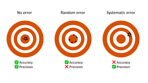
When you only have random error, if you measure the same thing multiple times, your measurements will tend to cluster or vary around the true value. Some values will be higher than the true score, while others will be lower. When you average out these measurements, you’ll get very close to the true score.
For this reason, random error isn’t considered a big problem when you’re collecting data from a large sample—the errors in different directions will cancel each other out when you calculate descriptive statistics. But it could affect the precision of your dataset when you have a small sample.
Systematic errors are much more problematic than random errors because they can skew your data to lead you to false conclusions. If you have systematic error, your measurements will be biased away from the true values. Ultimately, you might make a false positive or a false negative conclusion (a Type I or II error) about the relationship between the variables you’re studying.
Random error
Random error affects your measurements in unpredictable ways: your measurements are equally likely to be higher or lower than the true values.
In the graph below, the black line represents a perfect match between the true scores and observed scores of a scale. In an ideal world, all of your data would fall on exactly that line. The green dots represent the actual observed scores for each measurement with random error added.
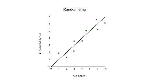
Random error is referred to as “noise”, because it blurs the true value (or the “signal”) of what’s being measured. Keeping random error low helps you collect precise data.
Sources of random errors
Some common sources of random error include:
- natural variations in real world or experimental contexts.
- imprecise or unreliable measurement instruments.
- individual differences between participants or units.
- poorly controlled experimental procedures.
| Random error source | Example |
|---|---|
| Natural variations in context | In an experiment about memory capacity, your participants are scheduled for memory tests at different times of day. However, some participants tend to perform better in the morning while others perform better later in the day, so your measurements do not reflect the true extent of memory capacity for each individual. |
| Imprecise instrument | You measure wrist circumference using a tape measure. But your tape measure is only accurate to the nearest half-centimeter, so you round each measurement up or down when you record data. |
| Individual differences | You ask participants to administer a safe electric shock to themselves and rate their pain level on a 7-point rating scale. Because pain is subjective, it’s hard to reliably measure. Some participants overstate their levels of pain, while others understate their levels of pain. |
What can proofreading do for your paper?
Scribbr editors not only correct grammar and spelling mistakes, but also strengthen your writing by making sure your paper is free of vague language, redundant words, and awkward phrasing.
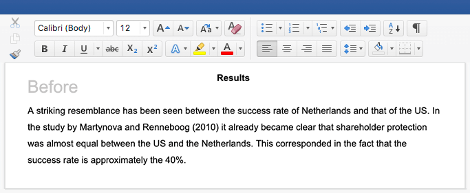
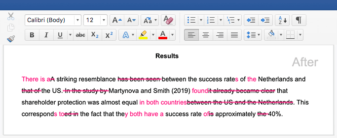
See editing example
Reducing random error
Random error is almost always present in research, even in highly controlled settings. While you can’t eradicate it completely, you can reduce random error using the following methods.
Take repeated measurements
A simple way to increase precision is by taking repeated measurements and using their average. For example, you might measure the wrist circumference of a participant three times and get slightly different lengths each time. Taking the mean of the three measurements, instead of using just one, brings you much closer to the true value.
Increase your sample size
Large samples have less random error than small samples. That’s because the errors in different directions cancel each other out more efficiently when you have more data points. Collecting data from a large sample increases precision and statistical power.
Control variables
In controlled experiments, you should carefully control any extraneous variables that could impact your measurements. These should be controlled for all participants so that you remove key sources of random error across the board.
Systematic error
Systematic error means that your measurements of the same thing will vary in predictable ways: every measurement will differ from the true measurement in the same direction, and even by the same amount in some cases.
Systematic error is also referred to as bias because your data is skewed in standardized ways that hide the true values. This may lead to inaccurate conclusions.
Types of systematic errors
Offset errors and scale factor errors are two quantifiable types of systematic error.
An offset error occurs when a scale isn’t calibrated to a correct zero point. It’s also called an additive error or a zero-setting error.
A scale factor error is when measurements consistently differ from the true value proportionally (e.g., by 10%). It’s also referred to as a correlational systematic error or a multiplier error.
You can plot offset errors and scale factor errors in graphs to identify their differences. In the graphs below, the black line shows when your observed value is the exact true value, and there is no random error.
The blue line is an offset error: it shifts all of your observed values upwards or downwards by a fixed amount (here, it’s one additional unit).
The pink line is a scale factor error: all of your observed values are multiplied by a factor—all values are shifted in the same direction by the same proportion, but by different absolute amounts.
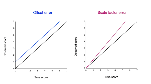
Sources of systematic errors
The sources of systematic error can range from your research materials to your data collection procedures and to your analysis techniques. This isn’t an exhaustive list of systematic error sources, because they can come from all aspects of research.
Response bias occurs when your research materials (e.g., questionnaires) prompt participants to answer or act in inauthentic ways through leading questions. For example, social desirability bias can lead participants try to conform to societal norms, even if that’s not how they truly feel.
Your question states: “Experts believe that only systematic actions can reduce the effects of climate change. Do you agree that individual actions are pointless?”
By citing “expert opinions,” this type of loaded question signals to participants that they should agree with the opinion or risk seeming ignorant. Participants may reluctantly respond that they agree with the statement even when they don’t.
Experimenter drift occurs when observers become fatigued, bored, or less motivated after long periods of data collection or coding, and they slowly depart from using standardized procedures in identifiable ways.
Initially, you code all subtle and obvious behaviors that fit your criteria as cooperative. But after spending days on this task, you only code extremely obviously helpful actions as cooperative.
You gradually move away from the original standard criteria for coding data, and your measurements become less reliable.
Sampling bias occurs when some members of a population are more likely to be included in your study than others. It reduces the generalizability of your findings, because your sample isn’t representative of the whole population.
Reducing systematic error
You can reduce systematic errors by implementing these methods in your study.
Triangulation
Triangulation means using multiple techniques to record observations so that you’re not relying on only one instrument or method.
For example, if you’re measuring stress levels, you can use survey responses, physiological recordings, and reaction times as indicators. You can check whether all three of these measurements converge or overlap to make sure that your results don’t depend on the exact instrument used.
Regular calibration
Calibrating an instrument means comparing what the instrument records with the true value of a known, standard quantity. Regularly calibrating your instrument with an accurate reference helps reduce the likelihood of systematic errors affecting your study.
You can also calibrate observers or researchers in terms of how they code or record data. Use standard protocols and routine checks to avoid experimenter drift.
Randomization
Probability sampling methods help ensure that your sample doesn’t systematically differ from the population.
In addition, if you’re doing an experiment, use random assignment to place participants into different treatment conditions. This helps counter bias by balancing participant characteristics across groups.
Masking
Wherever possible, you should hide the condition assignment from participants and researchers through masking (blinding).
Participants’ behaviors or responses can be influenced by experimenter expectancies and demand characteristics in the environment, so controlling these will help you reduce systematic bias.
Frequently asked questions about random and systematic error
-
What’s the difference between random and systematic error?
-
Random and systematic error are two types of measurement error.
Random error is a chance difference between the observed and true values of something (e.g., a researcher misreading a weighing scale records an incorrect measurement).
Systematic error is a consistent or proportional difference between the observed and true values of something (e.g., a miscalibrated scale consistently records weights as higher than they actually are).
-
Is random error or systematic error worse?
-
Systematic error is generally a bigger problem in research.
With random error, multiple measurements will tend to cluster around the true value. When you’re collecting data from a large sample, the errors in different directions will cancel each other out.
Systematic errors are much more problematic because they can skew your data away from the true value. This can lead you to false conclusions (Type I and II errors) about the relationship between the variables you’re studying.
Cite this Scribbr article
If you want to cite this source, you can copy and paste the citation or click the “Cite this Scribbr article” button to automatically add the citation to our free Citation Generator.
Bhandari, P.
(2022, December 05). Random vs. Systematic Error | Definition & Examples. Scribbr.
Retrieved February 9, 2023,
from https://www.scribbr.com/methodology/random-vs-systematic-error/
Is this article helpful?
You have already voted. Thanks 
Your vote is saved
Processing your vote…
Regression to the mean, RTM for short, is a statistical phenomenon which occurs when a variable that is in some sense unreliable or unstable is measured on two different occasions. Another way to put it is that RTM is to be expected whenever there is a less than perfect correlation between two measurements of the same thing. The most conspicuous consequence of RTM is that individuals who are far from the mean value of the distribution on first measurement tend to be noticeably closer to the mean on second measurement. As most variables aren’t perfectly stable over time, RTM is a more or less universal phenomenon.
In this post, I will attempt to explain why regression to the mean happens. I will also try to clarify certain common misconceptions about it, such as why RTM does not make people more average over time. Much of the post is devoted to demonstrating how RTM complicates group comparisons, and what can be done about it. My approach is didactic and I will repeat myself a lot, but I think that’s warranted given how often people are misled by this phenomenon.
Contents
- 1. Three types of RTM
- 1.1. Random measurement error
- 1.2. Sampling from the tails
- 1.3. Stable but nontransmissible influences
- 2. Measurement error and true score theory
- 2.1. Example: Donald’s IQ
- 3. Simulation: 10,000 IQ scores
- 4. Why is RTM stronger for more extreme scores?
- 5. Why RTM does not decrease variability: Egression from the mean
- 6. Estimating true scores
- 7. Will RTM go on forever?
- 8. Kelley’s paradox, or why unbiased measurement does not lead to unbiased prediction
- 8.1. Simulation: Black-white IQ gap
- 8.2. Simulation: Gender pay gap
- 9. Sampling from the tails
- 10. RTM due to reliable but non-transmissible influences
- 11. RTM and the etiology of IQ differences between groups
- 12. Discussion
- Notes
- References
- Appendix: R code
- Share this:
1. Three types of RTM
As I see it, there are three general reasons why RTM happens: random measurement error, sampling from the tails, and non-transmissibility of otherwise stable influences. I’ll briefly go over what I mean by them first.
1.1. Random measurement error
Any given variable will usually be measured somewhat imprecisely so that the values obtained do not necessarily correspond to the true underlying values. The extent to which a given observed value of the variable differs from the true value because of measurement error can be referred to as an error score. Error scores always “strike” individuals (or other units of analysis, e.g., companies, cities) randomly, and therefore are different from one occasion to another. If you get a large error score on first measurement, you will likely get a small one the next time simply because smaller error scores are more common than large ones. For example, if you take a difficult multiple-choice IQ test and make several correct guesses when you don’t know the answers, leading to you getting a very high test score, your score when retaking the test will likely regress towards the mean as you will probably not be as lucky with your guesses the second time around.
This graph demonstrates how IQ scores, represented by the grey dots, regress towards the mean in a large sample of individuals:

Figure 1.
IQ scores obtained on first testing are on the x-axis, while retest scores are on the y-axis. The test has a mean of 100 and a reliability of 0.80, and the red line is the line that best predicts an individual’s retest score based on his or her score in the first test. The blue lines with arrows highlight the varying magnitude of the regression effect at selected IQ levels. As can be seen, low and high scorers tend to be more average when retested. For example, those scoring 80 in the first test average about 84 in the second test, while the average retest score for those who scored 120 is 116. This (simulated) example is discussed in more detail later.
1.2. Sampling from the tails
Random measurement error is well-nigh inevitable, so some RTM due to it is guaranteed in most circumstances. However, in addition to random error, there are often other, more systematic influences that aren’t preserved from one measurement occasion to another, resulting in stronger RTM than is expected based on random error alone. In other words, variables may naturally show instability in their true, non-error values over time. If you are measured at a time when you are at your highest or lowest level (that is, close to the tails of the distribution) of such a variable, you are likely to regress to a more average value when remeasured.
For example, if you recruit patients suffering from depression for a clinical trial and measure their level of depression at the start of the treatment and at the end, you are likely to see them get better even if the treatment offered is completely ineffectual. This is because a disorder like depression is often episodic, with symptoms worsening and improving spontaneously over time. As patients usually seek treatment when their condition is at its worst, the mere passage of time often leads to some recovery regardless of any treatment. RTM in this case may happen not because of measurement error but because spontaneous improvement following a severe phase of the disease is a part of the normal course of the disease. Without a control group that doesn’t receive the treatment, you can never tell for sure if a patient would have got better untreated as well.
The following table (from Campbell & Kenny, 1999, p. 47) shows how the depression severity of patients assigned to no-treatment control groups in 19 clinical trials changed over the course of the trials. (Depression was measured using questionnaires like the Beck Depression Inventory.)
Table 1.
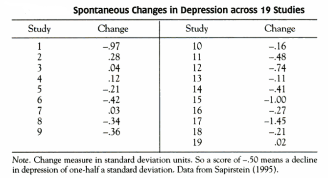
While there was variability between studies, depression levels decreased in 14 out of 19 studies for a mean decline of 0.35 standard deviation units. Most studies therefore saw RTM as untreated patients spontaneously got better.
1.3. Stable but nontransmissible influences
There are also variables that are temporally stable per se but nevertheless show RTM under certain conditions. The classic example of this is genetic transmission of traits in families. The graph below is from Galton (1886), which is a foundational study of RTM. Galton plotted the heights of mid-parents (that is, the average heights of spouses) against the heights of their children. He found that the children of very tall parents were shorter than them, while the children of very short parents were taller than them, on the average.
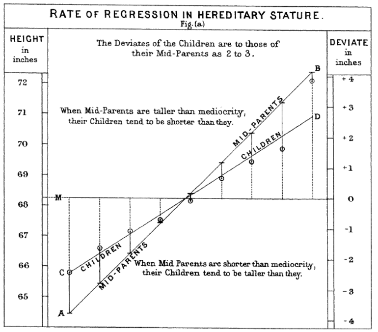
Figure 2.
Given that height is easy to measure accurately, random measurement error is rarely a major cause of RTM for height. The real explanation is that, as a general rule, parents can only transmit their additive genetic effects to their children. Other influences on parents’ own traits, such as non-additive genetic effects and accidents of individual development (e.g., a severe illness contracted early in life), will usually not be transmitted to children for lack of reliable mechanisms for such transmission. If parents have extreme phenotypic values due to other influences than additive genetic ones, those influences cannot be transmitted to their children who therefore tend to be phenotypically less extreme (more average) than their parents.
* * * *
In what follows, I will mostly employ the classical psychometric true score theory and random measurement error (case 1 above) to elucidate RTM, but I’ll also consider situations where RTM happens because of sampling from the tails (case 2) or because there are no mechanisms for transmitting otherwise stable influences (case 3).
2. Measurement error and true score theory
I’ll start by discussing the kind of RTM that is due to random measurement error. This is easiest to do from the perspective of true score theory. This theory is very general, so the variable of interest may be just about anything. It could be an IQ score, a measure of socioeconomic status, a blood pressure reading, whatever. However, I’ll be mostly using IQ in my examples because of its familiarity.
In true score theory, an individual’s measured value X for some variable of interest is modeled in terms of T, the true score, and E, the error score. X, called the observed score, is the sum of the two other variables:
X = T + E
In this equation, T represents a stable component that is reliably reproduced whenever the variable is measured. It could be, say, an individual’s underlying level of intelligence, if the variable in question is IQ.
In contrast to the stable and reliable true score, E is a random error component that is correlated neither with T nor with any new E component that is obtained if the variable is remeasured. In the case of IQ, E represents a conglomeration of ephemeral influences that may either boost (e.g., lucky guessing in a multiple-choice test) or impair (e.g., fatigue during test) your performance on one test occasion but will be absent and replaced with other influences if you retake the test. E can be thought of as noise that can prevent the observed score from accurately reflecting your true score. The smaller the influence of E on observed test scores is, the more reliable the test is. If error scores for all individuals were zero, the test would be perfectly reliable, and observed scores would be equal to true scores—something that is very rarely accomplished.
I will assume that both T and E are normally distributed and that E has a mean of 0 in the population. The normality of error scores may be violated in real-life data sets, but because the assumption is at least approximately true in many situations and it would be such a hassle for me to assume otherwise, I’ll ignore problems arising from non-normal error score distributions.
2.1. Example: Donald’s IQ
Let’s say we have a man, call him Donald, who takes an IQ test and gets a score of 125. This is his observed score in the test. In practice, the observed score is the only one of the three variables (X, T, E) introduced whose exact value can be known. The other two are hidden or latent variables whose values may only be estimated in various ways. But let’s assume that we somehow knew Donald’s true score and error score values to be T = 115 and E = 10. It can be readily seen that the observed score X equals 125 because X = T + E = 115 + 10 = 125.
If Donald were to retake an IQ test, what would be the best bet for his retest score? As T is the same (=115) across measurement occasions, the new observed score will be determined by E. Because error scores are uncorrelated with both true scores and previous error scores and normally distributed with a mean of 0, our best guess for Donald’s error score in the second test is 0, as it is the most common error score value. Therefore, the expected observed score in the second test is 115 + 0 = 115. If that happens, we have seen regression towards the population mean (which is 100 in the case of IQ)—an IQ of 125 shrunk to 115 upon retesting. The reason for the regression would be that only the reliable component (T=115) gets reproduced upon retesting, whereas the previously strongly positive error score (=10) is not reproduced because it does not represent a reliable, repeatable influence on IQ scores.
Of course, Donald’s error score in the second test may not be 0, but it is very likely that it is less than the original error score of 10 because error scores are normally distributed with a mean of zero, meaning that there’s a 50% chance that the error score is less than 0 and an even greater chance that it is less than 10. Given that Donald had an error score in the first test that took him further from the population mean than his true score is, RTM is to be expected in a retest.
As the example shows, people in fact regress towards their own true scores rather than towards the mean score of the population or sample. However, because true scores are unknowable quantities—in reality, we can’t really know Donald’s or anyone else’s true score—we have to settle for estimating what will happen on average, and on average people regress towards the mean because most people have true scores nearer to the mean than their observed scores are, as discussed in more detail later. Some people, of course, may not regress at all—they may get the same observed scores in two tests, or they may be further from the mean and/or from their true score in the second test—but on average RTM is what happens.
3. Simulation: 10,000 IQ scores
For a more involved look at how RTM happens in a large group of people, I generated simulated IQ scores for 10,000 individuals drawn from a population with a mean IQ of 100 and a standard deviation (SD) of 15. I chose a reliability of 0.80 for these scores. This means simply that 80% of the between-individual differences in the scores represent reliable, or true score (T), differences, while 20% of the between-individual differences are due to random measurement error (E).
The variance of the observed IQ scores is the square of their SD, or 15^2 = 225. Of this total variance, 80% or 180 is true score variance. The rest, 45, represents error score variance. By taking square roots of these variance components we get the SDs of the true scores and the error scores: √180 ≈ 13.42 and √45 ≈ 6.71, respectively.[Note] The SD of the error scores can be used to construct confidence intervals for the observed scores. With an SD of 6.71, the 95% confidence interval is ±1.96 * 6.71 ≈ ±13.5. Therefore, the observed IQs of 95% of test-takers will be within 13.5 points (in either direction) from their true scores.
To fully characterize the (normal) distributions of error scores and true scores, we need to know the means of each distribution. For error scores, it is 0, because negative and positive errors are equally likely, canceling each other for the average individual. The mean of the true scores is 100. This is so by my choice, but because 100 is the mean and thus the most common true score and 0 is the mean and thus the most common error score, the mean of the observed score distribution is necessarily 100 + 0 = 100, within the limits of sampling error.[Note]
Knowing the means and SDs of the true scores (100, 13.42) and the error scores (0, 6.71), we can get numbers matching these parameters from a random number generator and graph the resulting distributions, as shown in Figures 3 and 4:
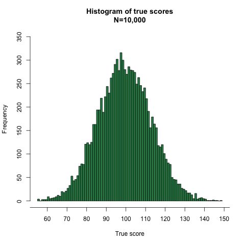 Figure 3.
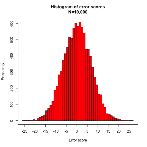
Figure 4.
(The R code for all of my graphs, simulations, and analyses is available in the Appendix.)
True scores are expected to be uncorrelated with error scores. We can verify this by correlating the simulated true and error scores, which produces a Pearson correlation of 0.001 (p=0.92). Error and true scores are not associated beyond chance levels. This is, of course, expected because the two variables were randomly generated.
The observed IQ scores were formed simply by summing the 10,000 true scores and 10,000 error scores: X = T + E. This gives the following distribution of 10,000 observed IQ scores with a mean of 100 and an SD of 15:

Figure 5.
Now that we have one set of IQ scores, we can simulate what would happen if the same 10,000 individuals took another IQ test. In the new test, the true score for each individual stays the same, but everyone gets a new error score generated randomly from a distribution that has, as before, a mean of 0 and an SD of 6.71. The results are plotted in Figure 6, with the gray dots representing test scores. On the x-axis we have the scores from the first test while the retest results are on the y-axis.
Figure 6.
The red line is the least squares fit line that best predicts scores in the second test based on scores in the first test. The slope of the line (its steepness) is 0.80.[Note] The regression equation for the red line gives the expected score in the retest, E(Xretest), for someone who scored X in the first test:
E(Xretest) = 20 + 0.8 * X
The blue lines with arrows in the graph highlight the degree of regression for selected observed scores. Those who scored 60 in the first test score 68, on average, in the second test, while those who scored 80 in the first test average 84 in the second. The blue lines also highlight two above-average scores in the first test, 120 and 140, and it can be seen that people who scored above average regress to the mean in a symmetrical fashion to those who scored below the mean. Notably, those scoring 60 or 140 in the first test experience more RTM than those who scored 80 or 120—the regression effect is stronger for more extreme scores. As to individuals whose scores in the first test were equal to the mean IQ of 100, they cannot, as a group, experience RTM, so they average 100 in the second test, too.
So, why does RTM happen for these simulated individuals? Let’s look again at the true scores and error scores that compose the observed scores:
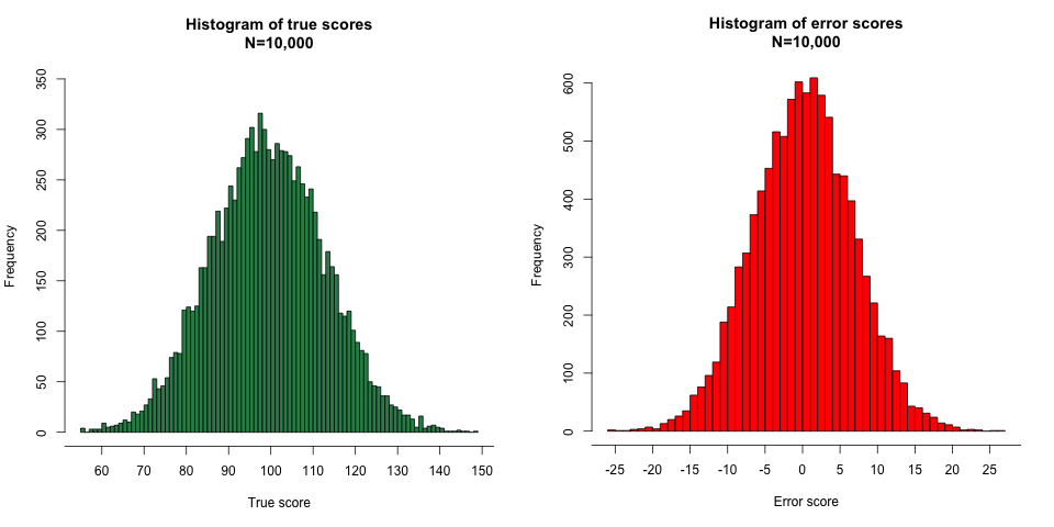
Figure 7.
In the first test, each individual has a true score (left-hand distribution in Figure 7) which is summed with a randomly selected error score from the error score distribution (right-hand distribution).Let’s say that you have a true score of 110 and get an error score of +20 in a test, resulting in an observed score of 130. In a normal distribution with a mean of 0 and an SD of 6.71, such an error score is 20/6.71 ≈ 3 SDs above the mean, corresponding to 99.9th percentile. Therefore, 999 out of 1000 people get smaller error scores than 20 in the test.
Now, if you retake the test, what’s the probability that you get a new error score that is smaller than 20? Because error scores are uncorrelated across tests, the probability of your getting a particular error score is the same as any person getting a particular error score, so your probability of getting an error score smaller than 20 is 99.9%. This means that you will almost certainly get a lower observed score in the retest, causing you to regress towards the population mean. Most likely, your error score will be within a handful of points from 0, given that 68% of error scores are within ±1 SD of the mean error score of 0, which in this case means between -6.71 and +6.71.
But what if your true score is, say, 70, and you get an error score of 20, for an observed IQ of 90? Will you regress towards 100 when retested? You probably will not. On the contrary, you will likely be further away from the mean in the second test, given that you’ll almost certainly get an error score smaller than 20. This underscores the fact that, firstly, RTM happens only on average. There are more people with true scores close to the mean than far from the mean, so on average people with large error scores tend to regress towards the mean when retested. Secondly, individuals actually regress towards their own true scores rather than the true score of the population or sample. The true scores of individuals, however, are unknown, whereas the mean true score is known (it is the same as the observed mean), so we use the mean to describe how RTM occurs for the average individual, because what happens to a particular individual in a retest cannot be predicted.
Another way to make RTM more transparent is to examine how individuals with a particular observed score regress in a retest. Table 2 shows everybody (N=31) from the simulation who scored 130 in the first test, along with their retest scores, error scores in both tests, and true scores.
| ID # | Observed score 1 | Observed score 2 | Error score 1 | Error score 2 | True score |
|---|---|---|---|---|---|
| 1 | 130 | 138 | -5.6 | 2.5 | 136 |
| 2 | 130 | 114 | 13.8 | -2.4 | 116 |
| 3 | 130 | 120 | 10.5 | 0.6 | 119 |
| 4 | 130 | 134 | -3.9 | -0.3 | 134 |
| 5 | 130 | 113 | 16.2 | -0.8 | 114 |
| 6 | 130 | 120 | -1.5 | -10.7 | 131 |
| 7 | 130 | 128 | 6.6 | 4.7 | 123 |
| 8 | 130 | 127 | 9.7 | 6.8 | 120 |
| 9 | 130 | 140 | -1.8 | 7.7 | 132 |
| 10 | 130 | 127 | 9 | 5.6 | 121 |
| 11 | 130 | 130 | 1.6 | 2.1 | 128 |
| 12 | 130 | 106 | 23.2 | -1.5 | 107 |
| 13 | 130 | 125 | 5.2 | -0.4 | 125 |
| 14 | 130 | 124 | 7.3 | 0.5 | 123 |
| 15 | 130 | 128 | 7.4 | 4.5 | 123 |
| 16 | 130 | 122 | 13.1 | 4.9 | 117 |
| 17 | 130 | 122 | 4.4 | -3.8 | 126 |
| 18 | 130 | 134 | 5 | 9.3 | 125 |
| 19 | 130 | 120 | 9.9 | -0.4 | 120 |
| 20 | 130 | 143 | 1.8 | 15.4 | 128 |
| 21 | 130 | 127 | 4.7 | 1.7 | 125 |
| 22 | 130 | 112 | 8.3 | -10.4 | 122 |
| 23 | 130 | 122 | 3.4 | -5.5 | 127 |
| 24 | 130 | 114 | 5.6 | -10.2 | 124 |
| 25 | 130 | 120 | 1.2 | -8.6 | 129 |
| 26 | 130 | 113 | 5.7 | -11 | 124 |
| 27 | 130 | 124 | 0.8 | -4.9 | 129 |
| 28 | 130 | 105 | 4.1 | -21.4 | 126 |
| 29 | 130 | 123 | 6.9 | 0.1 | 123 |
| 30 | 130 | 130 | 7.2 | 6.6 | 123 |
| 31 | 130 | 127 | 7.4 | 3.6 | 123 |
| Mean | 130 | 124 | 6.0 | -0.5 | 124 |
The last row of the table shows the mean values of each variable. Those who scored 130 in the first test tend to regress towards the mean, scoring an average of 124 in the retest. The mean error score in the first test was 6.0 points, while it’s about 0 in the retest (-0.5 to be precise). The mean retest error score is ~0 because 0 is the expected, or mean, error score that any group of people who are retested are going to converge on, regardless of their original scores. Because the mean retest error is ~0, the mean observed retest score is approximately equal to the mean true score.
The fact that the retest and true scores both average 124 does not mean that the mean error score of all people scoring 124 in the retest is ~0. Instead, the mean error score of all people scoring 124 is about +5, reflecting the fact that people getting observed scores above the population mean tend to have positive error scores. Only the subset of people who regressed from 130 to an average of 124 have a mean error score of ~0.
4. Why is RTM stronger for more extreme scores?
Error scores are uncorrelated with true scores. At every level of true scores, error scores are normally distributed with a mean of zero. In the IQ simulation, for example, whether your true score is 70 or 100 or 130, your error score is in any case drawn from a normal distribution with a mean of 0 and an SD of 6.71 points.[Note] Table 3 shows the means and SDs of error scores for selected true scores in the simulated data.
| True score | Mean error | SD of error | N |
|---|---|---|---|
| 60 | 2.4 | 11.51 | 3 |
| 70 | -0.4 | 6.69 | 21 |
| 80 | 0.1 | 6.81 | 121 |
| 90 | 0.5 | 6.61 | 222 |
| 100 | 0.6 | 6.73 | 280 |
| 110 | -0.7 | 6.69 | 241 |
| 120 | 0.7 | 6.57 | 101 |
| 130 | -2 | 7.13 | 25 |
| 140 | 0.7 | 5.18 | 5 |
Given that large errors (either positive or negative) are not more common among those with extreme true score values (except by chance), how is it possible that measurement error and therefore regression toward the mean especially affect scores that are located farther from the mean, at the tails of the distribution? Wouldn’t you expect negative and positive errors to cancel out at each true score level? Why does RTM happen at all if negative and positive error scores are balanced so that the average error is 0 across the board?
The answer to these questions is that while measurement error is uncorrelated with true scores, it is correlated with observed scores. This follows directly from the definition of observed scores. For example, if the reliability of a test is 0.80, it means that 20% of the variance of the observed scores is accounted for by measurement error. The correlation of error scores with observed scores is then √0.20 ~ 0.45—that is, small observed scores (e.g., IQ=70) tend to be associated with negative error scores, and large observed scores (e.g., IQ=130) with positive error scores. To put it another way, in the same sense that observed scores would be perfectly correlated with true scores save for the influence of error scores, observed scores would be perfectly correlated with error scores save for the influence of true scores. Table 4 shows the means and SDs of error scores for selected observed scores in the simulated IQ data.
| Observed score | Mean error | SD of error | N |
|---|---|---|---|
| 60 | -12.9 | 8.3 | 9 |
| 70 | -7 | 6.71 | 52 |
| 80 | -4 | 6.33 | 111 |
| 90 | -1.2 | 5.85 | 254 |
| 100 | -0.1 | 6.25 | 283 |
| 110 | 2.4 | 5.92 | 241 |
| 120 | 3.8 | 6.42 | 131 |
| 130 | 6 | 5.88 | 31 |
| 140 | 9.8 | 5.01 | 13 |
The smaller an observed score is, the more likely it is that its smallness is in part due to a negative error score. Conversely, the larger an observed score, the more likely it is that it is influenced by a positive error score. Plotting all observed scores against their associated error scores (Figure  makes the linear relation between the two apparent. Given that the correlation is ∼0.45, the scatter around the fit line is quite large but it is of similar magnitude across the range of observed score values.

Figure 8.
This idea is perhaps not obvious, so I’ll try to explain it in a more intuitive way. With normally distributed true scores and error scores, there are more true scores than observed scores nearer to the population mean. This can be seen in the following graph where the distributions of the true and observed scores from the simulated example are superimposed:
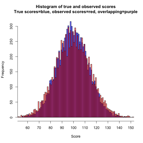
Figure 9.
The observed score distribution is broader and flatter than the true score distribution. There are comparatively fewer individuals with observed scores at the mean and more at the tails. When error scores are paired with true scores to form observed scores, true scores get, in a sense, pulled away from the mean because they “hang together” with their associated observed scores. Error scores are correlated with observed scores, with negative errors becoming more prevalent as you move from the mean towards smaller observed scores, and positive errors becoming more prevalent in the other direction from the mean.
For example, let’s say someone gets an observed IQ score of 80 in a population with a mean score of 100. Is his or her true score more likely to be smaller than 80 or larger than 80? The answer is that it’s probably >80 because there are more people with true scores in the range of, say, 80–90 who have negative error scores than there are people with true scores in the range of 70–80 with positive error scores—this is simply because of the shape of the normal distribution. To be precise, in a normal distribution of true scores with a mean 100 and an SD of 13.42[Note], 5.5% of scores are in the range of 70–80 while 16% are in the range of 80–90, corresponding to a ratio of 16/5.5 ~ 2.9. Given that true scores within each of these ranges are equally likely to be accompanied with negative and positive error scores, an observed score of 80 is more likely to be the sum of a true score of, say, 83 and an error score of -3 than it is to be due to a true score of 77 and an error score of +3—this is simply because there are more people with true scores of 83 than 77. When the individual who first scored 80 retakes the test, his or her new observed score is likely to be >80 because the underlying true score is likely to be >80 while the expected error score is 0—hence, regression towards the mean. This is so despite the fact that people with actual true scores of 80 are equally likely to have negative and positive error scores.
RTM gets weaker the closer you get to the population mean. This is because, as you approach the mean of the distribution, the number of true scores at each side of the observed score gets more even. For example, let’s say we have people with observed IQs of 90, the reliability still being 0.80. As noted, 16% of people have true scores in the range of 80–90. The proportion of true scores in the range of 90–100 is larger, 27%. The ratio of larger true scores to smaller true scores around the observed score of 90 is 1.7, compared to the ratio 2.9 around the observed score of 80. This means that RTM will be smaller for those scoring 90 compared to those scoring 80.
Finally, those scoring 100 in the first test will average 100 in the retest, experiencing no regression. This is because the number of true scores at either side of 100 is the same, meaning that an observed score of 100 is equally likely to result from a true score that is below 100 as from a true score than is above 100. Among those with observed scores of 100, those with true scores below 100 will likely score below 100 in a retest, while the opposite is true for those with true scores above 100. Thus, on average, there is no discernible RTM for those scoring 100.
To recap, RTM due to measurement error is caused by the fact that people with large (absolute) error scores on first measurement tend to have small (absolute) error scores on second measurement. Because small error scores are more common and error scores are uncorrelated across measurement occasions, most people will get small error scores upon remeasurement even if they got large scores the first time around.
People with extreme—positive or negative—observed scores tend to regress more toward the mean than people with less extreme observed scores. This happens because error scores are correlated with observed scores: large negative errors are common among those with very small observed scores, while large positive error scores are common among those with very large observed scores. RTM disproportionately affects extreme observed scores to the extent that they are caused by extreme error scores. In contrast, extreme observed scores that are caused by extreme true scores are not affected by RTM.
If mean, reliability and the SDs of observed and error scores are known, the average amount of RTM that people scoring X will experience in a retest can be predicted. If we assume that…
X = 130
mean = 100
reliability = 0.80
SDobserved = 15
SDerror = 6.71
… we can predict that the average amount of RTM will be about 6 points. This is because the correlation between observed and error scores is √0.20 ≈ 0.45, causing those with observed scores two SDs above the mean (=130) to have a mean error score of 0.45*2*6.71 ≈ 6. Because the expected error score in the retest is 0, the mean RTM effect will be 6 points, and people will regress from 130 to an average score of 124. The fact that the average amount of RTM is predictable for a given observed score can be exploited to compute so-called true score estimates, as discussed later.
5. Why RTM does not decrease variability: Egression from the mean
RTM causes extreme values of a variable to be less extreme when remeasured. You might therefore expect the variable to be less dispersed on the second measurement, with more values nearer to the mean and fewer at the tails. In fact, RTM does not lead to diminished variance. In my IQ simulation, for example, the variance is the same (15^2 = 225) on both testing occasions.
If the causal factors that generate variability do not change, variance will not change across measurement occasions. In my simulation, 80% of individual differences in IQ scores are due to true score differences and 20% due to error score differences whenever IQ is measured. This means that while people who got extreme scores in the first test will tend to be less extreme in the second test, other people will take those “available” extreme scores in the second test. Those other people can for the most part only come from among those who were less extreme in the first test. This means that RTM is accompanied by a countervailing phenomenon which could be called egression from the mean (‘egress’: to come or go out, to emerge).
Egression from the mean can be demonstrated using my simulated IQ data. In the graph below, the results from the second test are now on the x-axis while the results from the first test are on the y-axis. The arrowed blue lines highlight how people who got selected scores in the second test had scored in the first test.
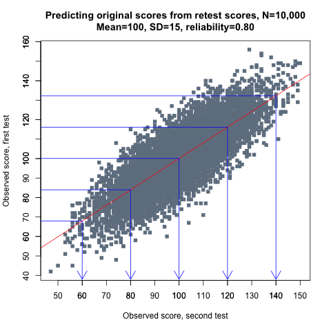
Figure 10.
This graph, with its time-reversed variable order, looks like a mirror image of the one presented earlier. The farther from the mean people scored in the retest, the more they egressed from the mean compared to their score in the first test, on average. For example, those who scored 60 in the retest had originally scored about 68, on average. Most people who scored around 68 in the first test didn’t egress to 60, of course—there are more people scoring 68 than 60 on every testing occasion, for one thing—but a subset of them did.
The egression effect is caused by people getting a more extreme (negative or positive) error score on remeasurement than originally. Given that error scores are “memoryless” in the sense that they are uncorrelated across measurement occasions, how is it possible that those with less extreme error scores on first measurement are more likely to get more extreme error scores when remeasured? In fact, they aren’t. The probability of extreme error scores is the same for everybody. Those who get extreme error scores and egress from the mean when remeasured tend to be drawn from among people who were originally closer to the mean for the simple reason that there are more people closer to the mean.
The egression effect is of the same magnitude but opposite to the regression effect. Egression effectively undoes RTM every time, maintaining the variance that exists. The complementarity of regression and egression underscores the fact that they are not forces for producing permanent change in a variable. Instead, regression and egression are ways to describe how the impact of transitory influences shifts from one group of people to another group of people. Regression and egression occur because there are temporary influences that impact different people over time.
As long as the population distribution of the variable does not change over time, RTM is always accompanied by egression from the mean. When a sample consists of individuals sampled from the tail(s) of the distribution—as in the case of depression patients described earlier—there appears to be no egression, but this is an artifact of selection bias. If the sampling frame of the study was, say, everybody who had an episode of depression during the last 12 months, rather than just people who recently sought treatment for depression, egression from the mean (i.e., people getting more depressed) would be observed and it would be equal in magnitude to RTM. The only way for this to not happen would be if the population prevalence of depression changed during the course of the study (because of, for example, new and more effective treatments).
Given that both regression and egression always happen, you might ask why RTM gets so much more attention. One reason is that many studies sample individuals from the extremes of the distribution—medical research focuses on sick rather than well people, psychologists like to study low-performing or high-performing people rather than average people, sociologists and economists are more interested in the poor and the rich rather than the middle class, and so on. This means that the samples studied will be, over time, strongly influenced by RTM while the effect of egression will be small.
Another reason for the focus on RTM is that egression introduces more error or other transitory influences on observed scores, whereas regression reduces unreliability, bringing the observed values closer to the stable underlying values.
6. Estimating true scores
The knowledge that observed scores tend to regress towards the mean makes it possible to predict what would happen if we obtained another set of observed scores for the same individuals even if no actual remeasurement takes place. Truman Kelley, who was an influential early psychometrician, introduced true score estimation for this purpose (see Kelley, 1923, p. 214ff, and Kelley 1927, p. 178ff; several of his books can be downloaded here). Kelley’s true score estimates, T’, are calculated in the following manner:
T' = M + ρ * (X - M)
where M is the population or sample mean, ρ is reliability, and X is the observed score. The purpose of this formula is to obtain scores that are closer to the true values than the observed scores are. It calculates how much a given observed score is expected to regress if remeasured, based on the known mean and reliability values, and assigns the expected regressed score as the best estimate of the true score. For example, if your observed IQ score is 130, the mean is 100, and the test’s reliability is 0.80, your estimated true score is T’ = 100 + 0.8 * (130 – 100) = 124.
An equivalent way of writing Kelley’s formula is:
T' = ρ * X + (1 - ρ) * M
This version of the equation makes it more explicit that the true score estimate is a weighted composite of the observed score (X) and the mean (M), with reliability ρ and 1 – ρ as weights. If we had a test that was completely unreliable, consisting of 100% measurement error, the estimated true score would be 0 * X + (1-0) * M = M. That is, if the test is just noise, with a reliability of 0, the best estimate for the individual’s true score is simply the population mean because it’s the only piece of information we have; the observed score is ignored because given a reliability of 0 it contains no information.
At the other end, if the test’s reliability is 1, the estimated true score is 1 * X + (1 – 1) * M = X. In other words, the estimated true score equals the observed score because an observed score in a perfectly reliable test equals the true score. In this case, the equation ignores the population mean value because we already get all the information we need from the observed score.
In practice, the reliability of a test is likely to be higher than 0 and lower than 1. For example, if the reliability is 0.50—that is, 50% of individual differences in observed scores are due to true score differences and 50% due to measurement error—the equation weighs the observed and mean scores equally, “pulling” the observed score half-way towards the mean—for example, the true score estimate for an IQ score of 130 would be 115. In contrast, if the reliability is, say, 0.90, the observed score will be pulled towards the mean by only 10% of the distance between the observed score and the population mean—for example, from 130 to 127.
In practice, estimated true scores are rarely used. Arthur Jensen and some other researchers in the same intellectual territory are the only ones I know of to have frequently used Kelley’s method in recent decades.
One reason for not using true score estimates is that they make group differences larger, as discussed below. Another reason might be that it’s not always clear what the relevant population mean score is. For example, let’s say we have a white person who scores 130 in an IQ test with a middling reliability of 0.80. If the white mean is 100, the true score estimate is 124. However, if the white person is Jewish, the true score estimate might be 126 instead, given a Jewish mean IQ of 110. In a stringent selection situation (for a school, job, etc.) those couple of points could make all the difference, making the choice of population mean very consequential.
A more technical or philosophical argument against Kelley’s formula is that it is a biased estimator. This means that the sampling distribution of estimated true scores is not centered on the actual true score. In other words, if you have a number of observed scores for an individual and you use Kelley’s method to estimate true scores for each observed score, the mean of those estimates is probably not equal to the individual’s true score (unless X = M). In contrast, the mean of the observed scores is centered on the true score, and if you have a number of observed scores (from parallel tests) for an individual, you can be confident that their mean is equal to the true score, within the limits of sampling error (that is, observed scores are unbiased).
Given that estimated true scores are biased in this way, why then prefer them over observed scores? The answer is that an estimated true score is, on the average, closer to the true score than an observed score is.[Note] This is because considering the mean of the population from which the individual is drawn together with his or her observed score effectively increases the reliability of the score. In my simulated IQ data the mean absolute error score for observed scores is 5.3 while it’s 4.8 for true score estimates. The advantage of true score estimates gets larger if we look at extreme scores. For example, when only considering those with observed scores below 80 or above 120 in the simulation, the mean absolute error score is 6.8 for observed scores, while it’s 4.7 for true score estimates. Furthermore, the more unreliable a variable is, the more can be gained by using true score estimates.
Because true scores estimates are linear transformations of observed scores, they correlate perfectly with the observed scores and therefore correlate with other variables just like the original, untransformed variable does. For this reason, if the purpose is not to interpret the scores on the original scale but to just rank individuals or to correlate the variable with other variables, nothing is gained by using true score estimates. However, true score estimates have an important function when groups with different mean levels for a variable are compared, as discussed later.
7. Will RTM go on forever?
So far, I’ve only examined situations where there are two measurements or tests. But what would happen if there were three or more sets of measurements of the same individuals? Would RTM go on and on, with individuals getting closer and closer to the mean with each measurement? As is obvious from the foregoing, that would not happen. For a given group of individuals, RTM is a one-off phenomenon, and it does not alter the population-level distributions of variables over time. If we select a group of individuals who obtained an extreme score when first measured, they will regress towards the mean when remeasured. If they are remeasured again, the statistical expectation is that they will, as a group, neither regress nor egress but stay where they were on the second measurement—and this will be true no matter how many times they are remeasured. This is because the expected error score for this group is always 0 after the first measurement; on the first measurement the expected error score was non-zero because by selecting individuals with extreme observed scores you essentially select individuals who have non-zero error scores.[Note]
It should be clarified that the idea of parallel tests, at least in the case of IQ, is more of a thought experiment than a model that you would expect to closely fit data from repeated tests. This is so because by taking a test people learn to be somewhat better at it, which means that their average score will be somewhat higher in a retest. However, often we have scores only from a single test administration, in which case the parallel test model offers a convenient way of thinking about how measurement error has affected those scores. Moreover, if there’s a reasonably long time interval—say, a year—between two test administrations, practice effects are expected to be very small. (On the other hand, if the interval is several years, we would expect individuals’ true scores to change in accordance with the well-known age trajectories in cognitive ability [e.g., Verhaeghen & Salthouse, 1997]. Even in that case, however, we would not expect the rank-order of individuals to change much.)
8. Kelley’s paradox, or why unbiased measurement does not lead to unbiased prediction
Let’s say you have two groups, and that after measuring some variable of interest X you find that the groups differ in their mean values for X. If you then remeasure X, people who previously got extreme values will now tend to get less extreme values because of measurement error and RTM. However, because individuals regress towards the mean value of the group they belong to (rather than towards some common grand mean), the expected amount of regression will depend on a given individual’s group membership. The upshot of this is that members of different groups who got similar values on first measurement will tend to get systematically different values on second measurement. Specifically, members of the group with a higher mean score will tend to get higher values than members of the other group. This is because a given observed score will tend to overestimate the true score of a member of the lower-scoring group when compared to a member of the higher-scoring group.
The fact that RTM occurs towards population-specific mean values leads to problems in situations where groups are compared. For example, many studies have investigated whether cognitive ability tests predict the school or job performance of white and black Americans in the same way. There’s long been concern that tests might be biased against blacks, resulting in fewer of them being admitted to selective colleges or hired by firms than would be fair given their abilities. However, the standard finding from studies on predictive bias is that to the extent that there is bias, it favors blacks: they tend to score lower on criterion measures, such as college grade-point averages and job performance evaluations, than whites who have identical IQ, SAT, or other such ability scores. This is in fact exactly what you would expect if both the tests and the criterion variables were internally unbiased with respect to race in the specific sense that psychometricians usually define internal bias.
This paradoxical phenomenon where internally unbiased tests and criterion measures lead to external bias, or biased prediction, was dubbed Kelley’s paradox by Wainer (2000). The name was chosen because the aforementioned Truman Kelley was the first to discuss how group mean values contain information that is not included in (unreliable) observed scores.[Note]
8.1. Simulation: Black-white IQ gap
I will next show through simulations how Kelley’s paradox works in the context of the black-white IQ gap. For white scores, I will use the same 10,000 IQ scores from before, with a mean of 100, an SD of 15, and a reliability of 0.80. For black scores, the SD and the reliability are 15 and 0.80, too, but the mean is 85, in accordance with the IQ gap that is usually observed between whites and blacks in America. Figure 11 shows the regressions of observed scores on true scores in the simulated blacks and whites.
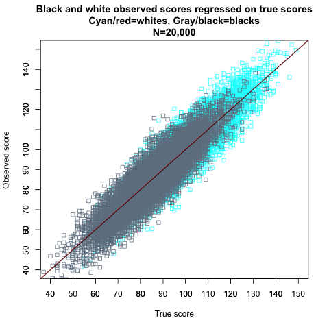
Figure 11.
The regressions are the same—the regression lines have the same slopes and intercepts—and therefore whites and blacks with the same true scores have the same observed scores, on average, with only random measurement error causing differences between individuals matched on true scores. This is in fact exactly the definition of strict measurement invariance, which is the term used when a test is internally unbiased with respect to particular groups, measuring the same construct (such as general intelligence) in the same way across groups. With strict invariance, the distribution of observed scores is identical for members of different groups who have the same true scores; everyone with the same true score gets the same observed score, within the limits of random measurement error (whose variance is the same across races).[Note] For example, if we choose all whites and all blacks with true scores of 115, both groups have a mean observed score of 115 and the same symmetrical dispersion around that mean due to measurement error.
Most people would probably agree that strict invariance is a reasonable indicator of a test’s internal unbiasedness, and that the IQs of my simulated blacks and whites are therefore “measured” without bias. However, if groups differ in their mean true scores, the following paradox arises even if strict invariance holds: Members of different groups with the same observed scores do not have the same distribution of true scores. If the population means differ, so will the regressions of true scores on observed scores. This can be demonstrated by flipping the variables from Figure 11 around (the red and black lines are the best-fit lines for whites and blacks, respectively):
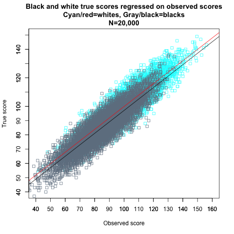
Figure 12.
In this scatterplot, observed scores for blacks and whites are used to predict their true scores. It can be seen that the slope coefficient (which indicates the “steepness” of the regression line) does not differ between groups—any change in observed scores results in the same amount of change in true scores in blacks and whites. However, it can also be seen that the intercepts—the locations where the regression lines intersect with the Y axis—differ between the races. The intercept difference indicates that the expected true score (Y axis) for any given observed score (X axis) is larger in whites than blacks.
From the regressions, we get the following equations for expected true score values, E(T), for whites and blacks at each level of the observed score X:
E(Twhites) = 20 + 0.80 * X

E(Tblacks) = 17 + 0.80 * X
At every IQ level, the underlying average true score for blacks is three points lower than that for whites. For example, if we choose all whites and all blacks with observed scores of 115, the mean true score of the white group will be 20 + 0.8 * 115 = 112, while the mean true score of the black group will be 17 + 0.8 * 115 = 109. This is Kelley’s paradox in action. The reason for this difference is that while the correlation between observed scores and error scores is the same, √0.20 ≈ 0.45, for both races, there’s a mean IQ difference between the two races. The expected error score for an observed score of 115 is 2 * 0.45 * 6.71 ≈ 6 for blacks, given that 115 is 2 SDs above the black mean of 85. For whites, the expected error score is 1 * 0.45 * 6.71 ≈ 3 because 115 is only 1 SD above the white mean of 100. The more extreme an observed score is, the larger its associated error score is, on the average, and an IQ of 115 is more extreme for blacks than whites. Another way to think of it is to observe that a larger proportion of whites than blacks scoring 115 have true scores that are at least that large.[Note]
Let’s say a selective college decides to grant admission to all applicants who score above 120 in an IQ test (this is not completely unrealistic considering that the SAT and the ACT are just IQ tests: Frey & Detterman, 2004; Koenig et al., 2008). Using the parameters from my simulation, we can expect that 9.1% of all whites will score above 120, while 6.8% of all whites will have true scores above 120. As for blacks, 1% are expected to score above 120, and 0.5% are expected to have true scores above 120. Therefore, roughly 6.8/9.1 ≈ 75% of whites with IQ scores above the cutoff will have true scores above the cutoff, while the same ratio is 0.5/1 = 50% for blacks. This means that even if the distributions of observed scores for those selected were the same for both races—which is unlikely—the true ability of the selected whites would still be higher than that of the selected blacks, resulting in racial differences in college performance.[Note]
Kelley’s paradox is not just a theoretical problem. It is frequently encountered in analyses of real-life data. For example, Hartigan & Wigdor (1989, p. 182) report that the intercept of the black prediction equation is lower than that for whites in 60 out of 72 studies that have examined whether the General Aptitude Test Battery (GATB) differentially predicts job performance across races. On the average, the GATB overpredicts black job performance by 0.24 SDs.[Note] Similarly, Mattern et al. (2008) report that in a sample of about 150,000 students, SAT scores overpredict first-year college GPA by 0.16 GPA points for blacks and by 0.10 GPA points for Hispanics when compared to whites. Braun & Jones (1981), Wightman & Muller (1990), and Wainer & Brown (2007) report comparable findings of pro-black and pro-non-Asian minority predictive bias based on the Graduate Management Admission Test, the Law School Admission Test, and the Medical College Admission Test, respectively. The finding is universal.[Note]
The irony of the pro-black and pro-non-Asian-minority bias that is inherent in cognitive tests given their less than 100% reliability is that the common belief is that they are biased against low-performing minorities. The “reverse” bias has long been recognized by psychometricians, but nothing has been done to address it. This is so despite the fact that the solution is simple: either use different prediction equations for each race, or use a method like Kelley’s formula to incorporate information about mean group differences in the model. Miller (1994) put it this way in his article where Kelley’s paradox is given a Bayesian interpretation:
“In plain English, once a test score has been obtained, the best ability estimate will depend on the average ability of the candidate’s group. Thus, if the goal is to select the best candidates, it will be necessary to consider group membership, and the mean ability of the candidate’s group. The general effect is to move the ability estimate for each candidate towards his group’s mean ability. When trying to select the best candidates (who will usually have evaluations above the mean for their group), the estimate for each candidate should be lowered by an amount that depends on mean and standard deviation for his group, and the estimate’s precision.”
For example, in my simulated data, transforming observed scores to true score estimates using race-specific means removes the intercept bias and therefore any overprediction that is due to measurement error, as seen in Figure 13 (compare to Figure 12).
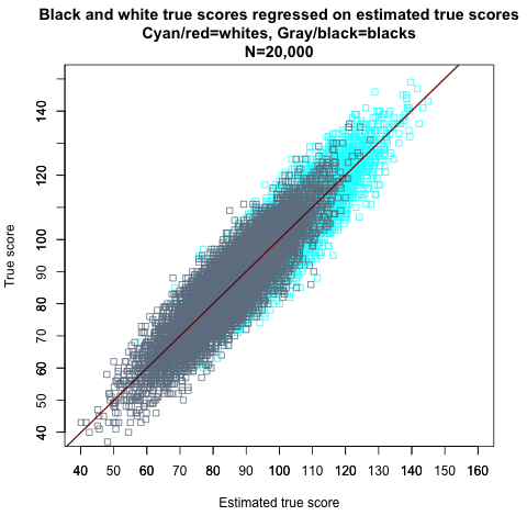
Figure 13.
The maxim that people should be treated as individuals rather than as members of groups frequently leads to unequitable treatment. For the sake of fairness, group membership should be considered together with individual characteristics wherever group differences exist. However, Linn (1984) articulated the reasons why corrections like Kelley’s formula are not used in practice:
“[I]t is not socially or politically viable to use different decision rules for members of different groups even if such a selection strategy is consistent with obtained differences in prediction systems. An important reason why this is so is that the bulk of the results of studies of differential prediction for minority and majority groups not only run counter to initial expectations and popular opinion, but they also run counter to the social goals that produced affirmative action policies. More specifically, the typical result, if interpreted within the context of the regression model, would generally require higher test scores for selection of minority group candidates than would be required of majority group candidates. Such an outcome is simply unacceptable.”
While the adoption of methods that adjust for the bias that favors low-performing groups in selection contexts is unlikely, such adjustments should nevertheless always be made in research contexts lest fallacious conclusions are drawn about discrimination. Unless a test is perfectly reliable, individuals with similar scores in it probably do not have equivalent true scores if they are drawn from populations that differ in their mean values for the variable.[Note]
8.2. Simulation: Gender pay gap
Kelley’s paradox can affect all kinds of variables, not just IQ, and it can affect several different variables simultaneously, which may produce predictive bias when methods like multiple regression analysis are used. While the biasing effect of measurement error on regression estimates is well recognized, it seems to me that the specific way in which it biases group comparisons is often not appreciated. Conceptualizing the bias in terms of Kelley’s paradox may make the phenomenon more transparent.
For example, it is well known that men earn, on the average, more money than women. It is also generally recognized that much of this gap can be explained by controlling for variables such as field of employment and hours worked. Usually such variables eliminate most of the gap, but if a residual gap remains, it is often attributed to gender-based discrimination. However, even assuming that all the relevant variables were really included in the analysis, it follows from Kelley’s paradox that the discrimination explanation is premature. Kelley’s paradox predicts that after regressing wages on all the variables that cause the gender gap there would still remain a gap, which, however, would be an artifact of measurement error.
I’ll simulate some data to demonstrate how Kelley’s paradox works with several independent variables. Let’s assume that the gender gap in weekly wages can be completely explained by four variables: hours worked, work experience, field of employment, and occupational level. For all these variables, men have higher average values than women, that is, the average man works more hours, has more work experience, is in a more remunerative field, and is more likely to be in a supervisory position, and so on, than the average woman.
Let’s say that the average weekly wages for full-time workers are $1000 for men and $780 for women, meaning that women earn 78 cents for every dollar men earn. Because wages are not normally distributed, I log-transform these figures, so that the average log wages are ln 1000 = 6.91 for men and ln 780 = 6.66 for women. The standard deviation for both sexes on the normally distributed log scale is, say, 0.7. These values yield the following simulated wage distributions for 10,000 men and 10,000 women:

Figure 14.
Table 5 shows correlations between wages, sex, and the four simulated explanatory variables, as well as the mean values and SDs of the variables for men and women. The explanatory variables are all distributed normally with a mean of 0 (men) or -0.25 (women) and an SD of 1 within sexes. Together the four variables explain all between-sex differences in wages, as well as 50% of within-sex differences (the remaining 50% is explained by unmeasured factors, e.g., education and IQ, which are ignored here as they are assumed to be uncorrelated with sex). The four variables are uncorrelated with each other within sexes, but there’s a small correlation (0.02) between them when sexes are pooled because men tend to have higher values than women. The prefix “true” indicates that the variables are error-free true score variables.
| Gender | Log weekly wage | True hours worked | True work experience | True field of employment | True occupational level | |
|---|---|---|---|---|---|---|
| Gender | 1 | |||||
| Log weekly wage | -0.18 | 1 | ||||
| True hours worked | -0.12 | 0.37 | 1 | |||
| True experience | -0.12 | 0.37 | 0.02 | 1 | ||
| True field of employment | -0.12 | 0.37 | 0.02 | 0.02 | 1 | |
| True occupational level | -0.12 | 0.37 | 0.02 | 0.02 | 0.02 | 1 |
| Male mean | 0 | 6.91 | 0.00 | 0.00 | 0.00 | 0.00 |
| Male SD | – | 0.70 | 1.00 | 1.00 | 1.00 | 1.00 |
| Female mean | 1 | 6.66 | -0.25 | -0.25 | -0.25 | -0.25 |
| Female SD | – | 0.70 | 1.00 | 1.00 | 1.00 | 1.00 |
The last rows of the table show that women’s mean values are 0.25 lower for all variables (other than the gender dummy variable where all men=0 and all women=1). This is so because women have 6.91 – 6.66 = 0.25 lower log wages. The sex differences in the four explanatory variables were chosen so that each explains a fourth of the gender pay gap and that they together explain all of it.
For starters, I regressed log weekly wages on the gender dummy variable. The unstandardized coefficient (B) of the variable, seen in Table 6 below, is -0.25 (p<0.001). Given that the dependent variable is logarithmic, this coefficient indicates that being a woman, as opposed to a man, is associated with an expected reduction of e^-0.25-1 ≈ -22% in wages, which is the gender pay gap specified above. Sex explains 3.1% of the variance in log weekly wages, corresponding to a correlation of -0.18 between wages and sex (the correlation is negative because men, who earn more on average, are coded as 0 and women as 1).
| DV: Log weekly wage | ||||
| B | 95% CI | p | ||
| (Intercept) | 6.91 | 6.90 – 6.92 | <.001 | |
| Gender | -0.25 | -0.27 – -0.23 | <.001 | |
| Observations | 20000 | |||
| R2 / adj. R2 | .031 / .031 |
Next, I regressed log weekly wages on the four explanatory variables and the dummy variable indicating gender. The results can be read from Table 7 below. Each of the explanatory variables accounts for a substantial amount of wage variance. The R^2 of the model is 52%. As expected, the coefficient of the gender variable is not significantly different from zero (p=0.728). This means that the four explanatory variables account for the entire sex effect on wages; the 22% gender gap is fully explained by sex differences in hours worked, work experience, field of employment, and occupational level.[Note]
| DV: Log weekly wage | ||||
| B | 95% CI | p | ||
| (Intercept) | 6.91 | 6.90 – 6.92 | <.001 | |
| True hours worked | 0.25 | 0.24 – 0.25 | <.001 | |
| True work experience | 0.25 | 0.24 – 0.25 | <.001 | |
| True field of employment | 0.25 | 0.24 – 0.25 | <.001 | |
| True occupational level | 0.25 | 0.24 – 0.25 | <.001 | |
| Gender | -0.00 | -0.02 – 0.01 | .728 | |
| Observations | 20000 | |||
| R2 / adj. R2 | .515 / .515 |
As noted, the explanatory variables are “true score” variables that are not contaminated by measurement error. Realistically, however, the variables would be measured with some error. Therefore, I transformed the true score variables into “observed”, error-laden variables by adding some random noise into them so that the reliability of each is 0.80. When I regressed log weekly wages on the four observed explanatory variables and the gender dummy variable, the results looked like this:
| DV: Log weekly wage | ||||
| B | 95% CI | p | ||
| (Intercept) | 6.91 | 6.90 – 6.92 | <.001 | |
| Observed hours worked | 0.20 | 0.19 – 0.20 | <.001 | |
| Observed work experience | 0.20 | 0.19 – 0.21 | <.001 | |
| Observed field of employment | 0.20 | 0.19 – 0.21 | <.001 | |
| Observed occupational level | 0.20 | 0.19 – 0.20 | <.001 | |
| Gender | -0.05 | -0.07 – -0.04 | <.001 | |
| Observations | 20000 | |||
| R2 / adj. R2 | .422 / .422 |
It can be seen, first, that the coefficients for each of the four explanatory variables are lower than in the previous model and the R^2 is also lower. This is a consequence of the added measurement error: less reliable variables explain less variance. More strikingly, the gender dummy, which was non-significant in the previous model, is now highly significant. In this model, there is a gender pay gap of e^-0.05-1 ≈ -5%, favoring men, even after controlling for the four explanatory variables.
The model reported in Table 8 and the variables used in it are exactly the same as in the model in Table 7 save for the random measurement error added to the independent variables. Therefore, we can conclude that the conditional gender pay gap of -5% suggested by the model is entirely spurious and artifactual, an example of Kelley’s paradox. The paradox affects the intercept of the regression equation, making it smaller for the group with lower mean values for the independent variables. In contrast, the slope coefficients are not (differentially) affected; they are equal for the two groups. This can be ascertained by running the model with interaction terms which allow the slopes to differ between sexes:
| DV: Log weekly wage | ||||
| B | 95% CI | p | ||
| (Intercept) | 6.91 | 6.90 – 6.92 | <.001 | |
| Observed hours worked | 0.20 | 0.19 – 0.20 | <.001 | |
| Observed work experience | 0.20 | 0.19 – 0.21 | <.001 | |
| Observed field of employment | 0.20 | 0.19 – 0.21 | <.001 | |
| Observed occupational level | 0.20 | 0.19 – 0.20 | <.001 | |
| Gender | -0.05 | -0.07 – -0.04 | <.001 | |
| Gender × obs hours | 0.00 | -0.01 – 0.01 | .906 | |
| Gender × obs experience | 0.00 | -0.01 – 0.01 | .912 | |
| Gender × obs field | 0.00 | -0.01 – 0.01 | .956 | |
| Gender × obs occupational level | -0.00 | -0.02 – 0.01 | .688 | |
| Observations | 20000 | |||
| R2 / adj. R2 | .422 / .422 |
None of the interaction terms (denoted by ×) are different from zero, confirming that measurement error only makes the intercepts, not the slopes, different between groups. This makes it easy to misinterpret the results as showing that while the independent variables predict higher wages for both groups in a similar, linear fashion, there is simultaneously a constant bias whereby women are paid less at all levels of the independent variables.
The artifact is caused by the fact that the true score value underlying any given observed value is smaller, on average, for women than for men. If the four explanatory variables were remeasured, both men and women would exhibit RTM, but women would regress to their own, lower means. This can be verified by separately regressing true scores on observed scores in men and women. The graph below shows the regressions for work experience (in z-score units), but the results are the same for all four variables.
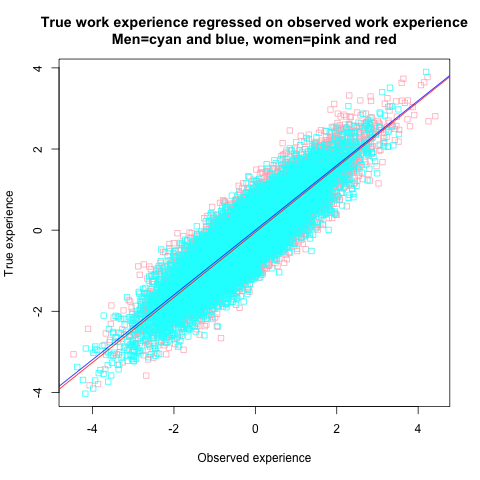
Figure 15.
While it may be difficult to discern from the graph, the intercept of the red female regression line is slightly lower than that of the blue male line. Specifically, the expected true work experience (T) predicted from observed work experience (X) is for men simply:
E(Tmen) = 0.80 * X
For women it’s:
E(Twomen) = -0.05 + 0.80 * X
Observed experience slightly overestimates the true experience that women have compared to men. This small intercept bias that is due to random measurement error causes, together with similar biases in the three other explanatory variables, the spurious gender pay gap of -5% seen in the regression model.
While the variables in my analysis are simulated, Kelley’s paradox is a plausible explanation for the residual gender pay gap found in many studies that have attempted to explain the gap by controlling for productivity-related variables. As few variables are measured without error, I don’t see how it could be otherwise. Nevertheless, this is rarely recognized in econometric literature where the pay gap is often studied, even though the effect of measurement error on parameter estimates is hardly something that econometricians are unaware of (even if they don’t use terminology like “Kelley’s paradox”). For example, in Blau & Kahn’s (2016) otherwise exhaustive analysis of the gender pay gap, it is acknowledged that the residual pay gap that remains after controlling for various covariates may be caused by unmeasured variables (rather than discrimination), but what is not discussed is the fact that a gap would remain even if all the relevant variables were included in the regression model and discrimination were non-existent. Measurement error introduces a bias in the estimates that is similar to the bias caused by omitted independent variables.[Note]
As usual, true score estimates based on sex-specific mean values can be used to adjust for the intercept bias introduced by measurement error.[Note] Table 10 shows that the use of true score estimates brings the unstandardized slope estimates very close to their true values (compare to Table 6), eliminating the spurious gender effect. (The R^2 of the model is not improved compared to models using observed scores because the within-gender correlation between true score estimates and observed scores is 1.)
| DV: Log weekly wage | ||||
| B | 95% CI | p | ||
| (Intercept) | 6.91 | 6.90 – 6.92 | <.001 | |
| Estimated true hours | 0.25 | 0.24 – 0.26 | <.001 | |
| Estimated true experience | 0.25 | 0.24 – 0.26 | <.001 | |
| Estimated true field of employment | 0.25 | 0.24 – 0.26 | <.001 | |
| Estimated true occupational level | 0.24 | 0.24 – 0.25 | <.001 | |
| Gender | -0.00 | -0.02 – 0.01 | .826 | |
| Observations | 20000 | |||
| R2 / adj. R2 | .422 / .422 |
9. Sampling from the tails
As I noted at the start of this post, RTM is not always caused by random measurement error. Sometimes individuals with extreme variable values regress towards the mean over time for reasons inherent to them and their circumstances that have nothing to do with measurement error.
Above, I used the example of people spontaneously recovering from depression. Another classic example of how “sampling from the tails” makes statistical analysis tricky is Horace Secrist’s (1881–1943) book The Triumph of Mediocrity in Business (1933). Secrist was a noted economist and statistician, but it did not prevent him from making the cardinal mistake of ignoring RTM. In the book, he analyzed the profitability of companies over years, showing that firms that are highly profitable or non-profitable in a particular year tend to become more mediocre in subsequent years. From these data, he concluded that economic life was characterized by increasing mediocrity.
Secrist’s results are of course just another example of regression (and egression): if we examine a group of companies with particularly high or low earnings this year, they will tend to become more mediocre in the following years, as this year’s particularly lucky or unlucky circumstances fade away (meanwhile, other companies “inherit” that good or bad luck). The unstable element that makes a company’s profits extreme is analogous to measurement error, but it is not caused by limitations in measurement instruments and is not noise in that sense (it’s hard, cold cash or lack thereof).
10. RTM due to reliable but non-transmissible influences
Thus far, we’ve dealt in more or less detail with RTM cases where the non-reliable component of a variable either consists of random error or is due to within-subject changes in true scores over time. However, RTM can exert a strong influence even when a variable’s value is stable within individuals and not much affected by measurement error. A classic example of such a process is familial resemblance in phenotypic traits.
Between-individual differences in a given human trait can, at least in principle, be decomposed into variance components in roughly the following manner, assuming that, like most (adult) human traits, this trait is not significantly influenced by shared (familial) environmental effects, and that the different influences are normally distributed and independent of each other:
VX = VA + VD + VE1 + VE2
where
V = variance
X = individuals’ trait values
A = individuals’ additive genetic values (summed across the genome)
D = individuals’ dominance values (values due to genetic interactions at the same loci summed across the genome)
E1 = values representing non-genetic influences unshared between relatives (e.g., accidents, “developmental noise”)
E2 = random measurement error scores
(E1 and E2 are usually rolled into one single non-shared environmental component, but for illustrative purposes they’re separated here.)
Let’s say that some trait fits this model (in each generation), and its additive genetic variance (VA) is 0.60, while dominance variance (VD) is 0.20, and the variances of E1 and E2 are 0.10 each. The variances sum up to 1, which is the variance of the phenotypic values (VX). Because of the scale chosen, the variances can be treated as standardized, e.g., VA=0.60 means that narrow-sense heritability is 60%. The means for X, A, D, E1, and E2 are all 0. A further assumption is that mating is random with respect to this trait.
Now let’s say that there’s a couple with extreme trait values (X). The couple’s average trait value, called the midparent value, is 2 SDs above the population mean (that is, Xmidparent = 2). What would you expect the trait values of their children be?
To answer that question, we need, first, to know what caused the parents to have such extreme trait values. We cannot know the answer for certain. This is because X = 2 can result from different combinations of influences. Sometimes people have high trait values because their genetic values are high, other times it’s because they have high non-genetic or measurement error values. Therefore, we have to settle for the answerable question of why parents who score X = 2 do so on average.
We know the causal model for how A, D, E1, and E2 give rise to different values of X:
X = A + D + E1 + E2
When the variances of dependent and independent variables are equal, as in the case of parallel tests discussed before, the regression slope is the same regardless of which variable is dependent and which is independent. The slope equals the correlation, and the expected deviation from the mean of either variable conditional on the deviation value of the other equals the product of the correlation and that conditional value, as expressed in Kelley’s true score formula. If the variances aren’t equal, as is the case here, the formula is slightly more elaborate (Campbell & Kenny, 1999, p. 26). For example, the expected value of A conditional on given values of X is given by:
E(A) = MA + corrA, X * (SDA / SDX) * (X - MX)
where M refers to the variables’ mean values. Given that the means of A and X are 0, the equation simplifies to:
E(A) = corrA, X * SDA / SDX * X
The correlation between A and X is √0.6 because A explains 60% of X’s variance. The SD of A is also √0.6. Therefore, the expected value of A conditional on X is:
E(A) = √0.6 * √0.6 / 1 * X = 0.6 * X
The expected values of D, E1, and E2 can be calculated in the same way. Because A, D, E1, and E2 are independent of each other, their expected values do not depend on each other. The expected values of D, E1, and E2 are:
E(D) = 0.2 * X
E(E1) = 0.1 * X
E(E2) = 0.1 * X
The expected values for A, D, E1, and E2 for a given level of X are therefore obtained simply by multiplying the variances of each with X. If X = 2, then:
E(A) = 0.6 * 2 = 1.2
E(D) = 0.2 * 2 = 0.4
E(E1) = 0.1 * 2 = 0.2
E(E2) = 0.1 * 2 = 0.2
These are the average midparent values when Xmidparent = 2.
The next question is how these values of A, D, E1, and E2 are transmitted over generations. Let’s look at the environmental components first.
E1 is an environmental or, more broadly, non-genetic component that affects only a specific individual; related individuals are not more similar on E1 than unrelated individuals. It is the set of unique trait-relevant experiences and influences that the individual has faced in his or her life. Therefore, parents’ E1 values cannot influence their offspring’s trait values, and children have an expected value of 0 for E1, 0 being the mean of E1’s population distribution.
Secondly, E2 is a random measurement error component. It is something that does not carry over even between different measurement occasions for the same individual, so parents’ E2 values also cannot influence their children. The expected value of the offspring for E2 is therefore 0.
With only the A and D components remaining, it’s clear that parent-offspring resemblance is determined solely by genetic influences. From quantitative genetic theory we know that different components of genetic variance cause similarities between parents and offspring in the following manner (from Falconer & Mackay, 1996, p. 155; note that the “parent” in the offspring-parent covariance can be either one parent or the midparent):
Table 11.

The model specified earlier includes additive variance, VA, and dominance variance, VD. The other variance components mentioned in the table do not contribute to the variance of the trait.[Note] As the table indicates, VA contributes to parent-offspring resemblance while VD does not. The covariance of offspring and parents for X is therefore simply 0.5 * VA = 0.5 * 0.6 = 0.3.
Now, to calculate the expected offspring trait values for given midparent trait values, we regress offspring values on midparent values:
E(Xoffspring) = B * Xmidparent
The slope coefficient B is equal to the covariance of Xoffspring and Xmidparent divided by the variance of Xmidparent. The variance of midparent X values is half the variance of individual X values. Therefore, B = 0.3 / 0.5 = 0.6. The expected phenotypic trait value of the offspring is 0.6 * Xmidparent.
B equals the additive heritability of the trait, which is not a coincidence: when there are no shared environmental influences (or epistasis), the regression of offspring trait values on midparent trait values equals heritability.
The breeder’s equation condenses the foregoing considerations into a simple formula:
R = h^2 * S
where
R = response to selection
h^2 = additive heritability
S = selection differential
Now consider again our couple whose midparent phenotypic value X is +2 SDs above the population mean while narrow-sense heritability is 0.6. Applying the formula, we get R = 0.6 * 2 = 1.2. This means that, on average, parents who score 2 SDs above the mean will have children who score only 1.2 SDs above the mean. RTM happens in this situation because only the additive genetic effects on parents’ traits are passed on to children. (The additive genetic values of children are, on average, equal to those of their midparent. The additive genetic value is for this reason also called the breeding value.) For parents with Xmidparent = 2, the average midparent values for D, E1, and E2 are 0.4, 0.2, and 0.2, respectively. Given that the additive genetic component is uncorrelated with the other components (D, E1, and E2) in the population, the offspring’s expected values for those other components are equal to population mean values, 0, causing them to regress compared to their parents. In short, when Xmidparent = A + D + E1 + E2 = 1.2 + 0.4 + 0.2 + 0.2 = 2, then E(Xoffspring) = 1.2 + 0 + 0 + 0 = 1.2.
If the offspring generation of the example were to have children with each other randomly and endogamously, their children would not regress towards the grand population mean of 0. Instead, the mean X of the grandchild generation would be 1.2, the same as that of their parents. This is because the non-transmissible influences on X, namely D, E1, and E2, are 0, on average, in the first offspring generation, precluding RTM from happening in subsequent generations. If this group of people continues to mate randomly and endogamously over generations, their mean X will remain at 1.2 perpetually (provided that the causal model underlying X does not change with time).
To recap, according to my model—which, while a simplification, fits lots of real-life traits reasonably closely—parents cannot transmit other influences on traits than additive genetic ones to their children. This causes the children of parents with extreme phenotypic values to regress towards the population mean by an amount that can be predicted using the breeder’s equation. This is so despite the fact that those other influences, except for measurement error, are more or less stable and not subject to RTM effects in the parents themselves.
11. RTM and the etiology of IQ differences between groups
Arthur Jensen noted a long time ago that when you match black and white individuals on IQ (or, preferably, on true score estimates of IQ), and then compare the IQs of these individuals to the IQs of their siblings, you will notice that the siblings of the black individuals will score lower than the siblings of the white individuals. Statistically, black and white siblings regress towards different means, and these regressions appear to be quite linear across the range of ability. For example, Murray (1999) reported regressions where blacks and whites from various NLSY surveys were grouped into a handful of IQ ranges (e.g., those scoring around 70, around 80, around 90, etc.) based on AFQT and PPVT scores and these group IQs were used to predict the IQs of the group members’ siblings. The following graphs show Murray’s results, with each dot representing something like a dozen to a hundred pairs of siblings:
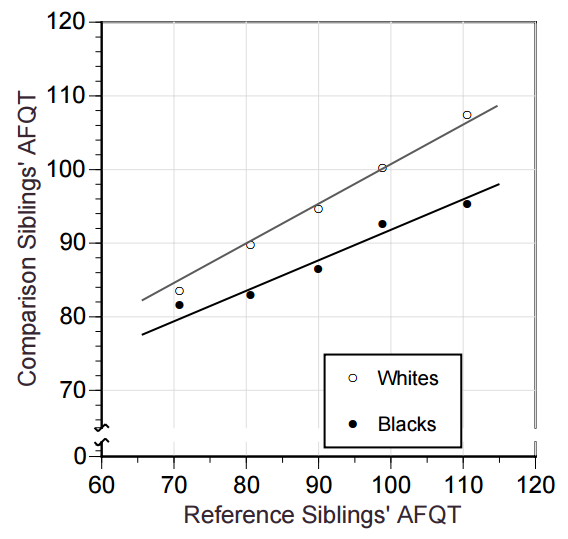
Figure 16.
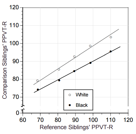
Figure 17.
Jensen argued that the different regressions provide evidence for his hereditarian explanation of the black-white IQ gap. His critics, however, have countered that the regressions towards different means could be due to environmental mechanisms.
From Table 11 in the previous section we find out that the genetic covariance of siblings equals 0.5 * additive genetic variance plus fractional (and usually substantively small to non-existent) contributions from genetic interaction components. This means that the correlation between siblings (monozygotic twins excepted) is much less than 1 and usually less than 0.5, unless the shared environment has a strong influence (which it hasn’t after childhood). This less than perfect correlation leads to RTM whereby the siblings of individuals with IQs far from the population mean score much closer to the mean. Given that the mean IQ of blacks is about 15 points lower than that of whites, we see the phenomenon illustrated in Figures 16 and 17.
Let’s say that the sibling correlation for IQ is 0.4. The following equation, where M is the population mean, gives the expected comparison sibling IQ based on the reference sibling’s IQ:
E(IQcomparison sib) = M + 0.4 * (IQreference sib - M)
It’s clear that if the reference individuals—those whose IQs are matched—come from populations with different mean IQs, their siblings will not have the same expected IQs. RTM “pulls” the IQs of the comparison siblings towards the respective means of the two populations.
Results like Murray’s above are a reflection of the fact that there’s a similar linear relation between sibling IQ scores in blacks and whites. The differential regression effect results from the fact that that only the familial component is shared between siblings whereas the non-familial, “non-transmissible” components aren’t. The farther from the mean an IQ score is, the more likely it is that it is strongly influenced by those non-transmissible influences. For this reason, the comparison siblings statistically regress towards the relevant population means.
The familial component of IQ variance appears to be overwhelmingly and roughly equally genetic in blacks and whites. This suggests that the regression effect is due to black-white differences in the genes underlying IQ.
Of course, it’s possible to argue that the mean value of the familial component is actually the same in blacks and whites and that differential regression happens because blacks are disadvantaged on the non-familial component, or that there’s a constant non-genetic “X-factor” that causes the gap. As I’ve argued elsewhere, such environmental explanations, if properly formalized, will face great difficulties in explaining the facts at hand. Nevertheless, the regression effect as such is only consistent with the genetic explanation; other models might explain the gap as well. Structural equation models that incorporate group means could take the discussion about the regression effect and its causal implications further, as was done in Rowe and Cleveland’s (1996) small pilot study. Unfortunately, after David Rowe’s untimely death no one has pursued this line of research.[Note]
12. Discussion
Selecting individuals who have extreme variable values usually means selecting observations that are biased by larger than usual amounts of measurement error or other transient, unstable influences. If you remeasure the variable, such selected individuals are likely to regress towards the mean because the transient influences that caused many of them to have extreme values earlier are now absent. This is the mechanism underlying the phenomenon of regression to the mean.
RTM by itself does not cause permanent change in the distribution of a variable’s values. When some individuals regress towards the mean upon remeasurement, others egress away from the mean, taking the places that those “regressed” individuals previously occupied in the distribution. Regression and egression are terms given to transitory influences that affect different people over time.
Measurement error makes group comparisons challenging in situations where groups’ mean values for the variable(s) of interest differ. Kelley’s paradox refers to the fact that measurement error causes the observed values of groups with low mean values to overestimate true values when compared to the observed values of groups with high mean values. This results in the overprediction of the low-scoring groups’ performance. I used the black-white IQ gap and the gender pay gap to demonstrate Kelley’s paradox, but the phenomenon is entirely general and can affect any kinds of groups and variables.[Note]
Group mean values contain information that is not included in unreliable observed variable values. This means that even when you have access to individuating information, it does not make sense, from a strictly statistical perspective, to treat individuals from different groups in the same way if the groups have substantially different mean values for the variables of interest. If you match individuals on observed variable values, individuals from groups with higher mean values are likely to have higher true score values than individuals from groups with lower mean values. Using true score estimates instead of observed scores is one way of adjusting for this bias. True score estimates work because they are based on the statistical certainty that unreliable observed scores regress towards their true values and the mean if remeasured.
RTM often happens because observations are sampled from the tails of the distribution. Upon remeasurement, individuals (or other units of analysis) with extreme values may regress towards the mean not only because of measurement error, but also because it is in the nature of the variable’s true score values to be unstable within individuals. When repeated measurements of such variables are taken, it is fallacious to attribute changes in variable values to external causes if natural variability is not accounted for.
The regression of offspring towards the population mean from the phenotypic values of their parents is an observation that helped Francis Galton discover the general statistical phenomenon of RTM. Familial regression is caused by the fact that expected familial resemblance in most phenotypic traits is almost completely determined by additive genetic influences (except in monozygotic twins who share just about all genetic effects, including non-additive ones). Other influences than additive genetic ones always contribute to trait variation, and (adult) family members are usually no more similar with respect to those other influences than random strangers in the same population. To the extent that individuals’ extreme trait values are not determined by their extreme additive genetic values, their relatives will, on average, have trait values that are less extreme and closer to the population mean. The breeder’s equation is a simple formula that can be used to predict the magnitude of the familial regression effect.
Notes
1. While observed scores are formed by summing true and error scores, the sum of the SDs of the latter two—13.42+6.71=20.13 here—does not equal the observed SD of 15. This is because SDs, unlike variances, are not additive. To get the SD of the observed scores, you take the square root of the sum of the true and error variances: √(13.42^2+6.71^2)=15.
2. Emil Kirkegaard, who read a draft of this post, pointed out that continuous distributions don’t have “most common values”. I admit that the language I’ve used in this post may be mathematically loose in places, but I’m trying to make my arguments widely accessible, so more intuitive explanations take precedence even if they aren’t always technically quite accurate. In any case, I generally use values of true and observed scores that are rounded to closest integers, so those distributions are in effect discrete.
3. Given that the variances of the first and second tests are the same (namely, 15^2=225), the slope is equal to the correlation between the two. The reliability of the test is also 0.80, which is not a coincidence. The traditional psychometric definition of reliability is that it is the correlation between two parallel tests, parallel tests being tests that measure the same true scores with the same reliability.
The fact that the reliability of parallel tests is equal to the correlation between them is easy to grasp when you draw a path diagram of the relationships between (standardized) true scores and tests:
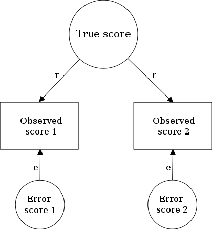
In this diagram, the correlation of true scores with observed scores in either test is r. The reliability of the tests is the proportion of variance that true scores explain in them, or r^2. Tracing rules for path diagrams tell us that the correlation between the parallel tests is r*r = r^2, which equals the reliability.
4. The SD is 13.42 rather than 15 because it’s the true score distribution which is narrower than the observed score distribution. SD=13.42 corresponds to a reliability of 0.80 because √(0.8*(15^2))~13.42.
5. Error scores and true scores are uncorrelated by definition in true score theory and therefore also in my simulations. In practice, it is possible that the reliability of a test or other variable varies as a function of true score level. For example, an IQ test may not contain sufficient numbers of items for each ability level. Such problems, which can be addressed with item response theory models, are ignored in this post.
6. Kelley’s true score formula, like all shrinkage estimators, trades off unbiasedness for lower mean estimation error. Psychometrics has always developed somewhat independently of “mainstream” statistical science, so it’s interesting that Kelley’s formula actually predates the development of shrinkage estimation by Charles Stein and others by several decades. This is another example of what Andrew Gelman has called a “longstanding principle in statistics”: Whatever you do, somebody in psychometrics already did it long before.
7. If you have results from two or more parallel tests, you can construct more reliable observed scores by summing the scores across tests. In my simulated data, the correlation between true scores and the sums of the two observed scores is 0.943. Squaring it, we get ~0.89, which is the reliability of the sum scores.
The reliability of such sum scores can also be estimated analytically. The Spearman-Brown prediction formula gives an estimate of how much reliability increases when you multiply the length of a test. In the case of two parallel tests with a reliability of 0.80, the Spearman-Brown estimate for the reliability of their sum scores is 2*0.8/(1+(2-1)*0.8) ≈ 0.89, matching the simulated example.
8. I’m not sure who first recognized the existence of Kelley’s paradox. It is implicit in Kelley’s own writings in the 1920s, but I haven’t found an explicit discussion of it in them. It was in any case acknowledged early on in psychometrics, because a 1942 article about the paradox in Psychometrika starts with a disclaimer that the article is “in the nature of a reminder of old truths, rather than a message of startling novelty” (Thorndike, 1942). More modern treatments include Jensen (1980, pp. 94–95, 275–277, 383–386), Linn (1984), and Millsap (1998, 2007).
9. It may help to understand why the intercept bias happens when true scores are regressed on observed scores but not the other way round if you remember that in regression analysis random measurement error in the independent variable(s) biases the estimates downwards while error in the dependent variable does not bias the estimates (it only increases their standard errors). If you standardize your variables, as in correlation analysis, measurement error will bias the estimates regardless of which variable is affected by it.
10. A simplification in this post is that I treat the true scores underlying a test as unitary. In practice, the reliable portion of a test’s variance is almost always multidimensional. For example, while IQ scores mostly reflect g variance, they are always “flavored” by the specific tests used, the more so the less diverse the test battery is.
Gignac (2015) factor-analyzed Raven’s Progressive Matrices together with many other tests taken by the same individuals. He found that when he decomposed Raven’s scores into orthogonal sources of variance that they shared with scores from other tests, the variance of the Raven’s scores was approximately 50% due to g and 10% due to fluid intelligence, while an additional 25% was due to variance specific to the Raven’s test. This comes up to 85%, meaning that 15% of Raven’s matrices variance was due to measurement error in this sample. The true score variance of the Raven’s was 85%, which, however, cannot be treated as coterminous with any single latent construct because of its underlying multidimensionality.
In the case of one population, it seems to me that little is loss in terms of generality when true scores are treated as unitary when discussing RTM—what is reliable is reliable regardless of what it precisely is. However, when there are group differences and only some portion of the reliable variance—for example, only the g variance of Raven’s scores—is correlated with both criterion outcomes and group differences, Kelley’s paradox may have a larger effect than what one would predict based on test-retest reliability. For simplicity’s sake, I have ignored the multidimensionality of true scores in this post.
11. For real data, true scores are never available, unlike in my simulation. When measurement invariance is examined in real data sets, true scores are assumed to be equal to the shared variance of the observed variables that are used as indicators of the true underlying variable. For example, the shared variance of a number of different cognitive ability tests may be assumed to be equal to a latent true score variable labeled as general intelligence, or g. The larger the number of indicator variables that are used, the less there is psychometric sampling error and the more accurately the underlying true score variable is captured.
12. The intercept difference was statistically significant in 26 of the 72 GATB studies. In 25 of them the black intercept was smaller, while the white intercept was smaller in one study. Many of the individual studies were rather small, with as few as 50 workers from each race, so it is not surprising that there aren’t always significant differences.
13. It’s possible that overprediction is not solely due to Kelley’s paradox. It could also be due to biased criterion variables or due to influences other than IQ that correlate with both the criterion variables and race. However, the presence of mean group differences and unreliability in the independent variable is always expected to result in at least some differential prediction.
14. True score estimates inflate any group differences that exist. This happens not because Kelley’s formula changes group means (it doesn’t) but because it decreases within-group variances by assuming that everybody—rather than just the average person—who scored X in the first test would regress to the same score in a retest. In the simulation, the observed IQ difference between blacks and whites is 15 points, or 1 SD, while the true score difference is larger, namely 15/13.42 ≈ 1.12 SDs. The gap in true score estimates is even larger because the SD is only 12—15/12 = 1.25 SDs. The upside to this bias is, however, that when used in selection settings, true score estimates eliminate group differences in sensitivity, or the true positive rate, as shown in Figure 11 above.
An additional problem in selection is that the specificity (aka the true negative rate) of observed scores is lower in the group with a higher mean score. Borsboom et al. (2008) illustrate how Kelley’s paradox leads to differences in sensitivity and specificity between high-scoring (H) and low-scoring (L) groups in the following way:
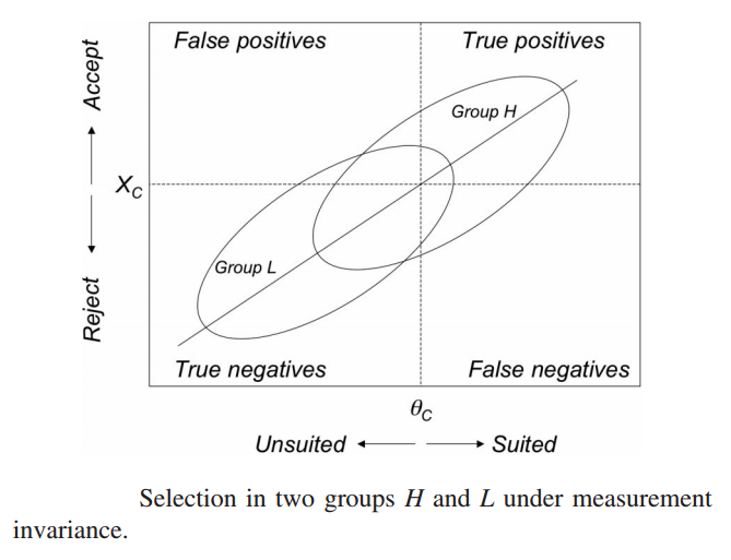
Point Xc on the y-axis represents the selection decision cut-off point based on observed scores, while point θc on the x-axis shows the true score cut-off point. Compare the ratios of H and L groups, whose distributions are represented by the two ellipses, in different quadrants. For example, the majority of accepted H group members are true positives while the majority of accepted L group members are false positives. The exact magnitude of these biases depends on factors such as the size of the group difference and how stringent selection is, but some bias is always expected when the test used is unreliable and there are group differences in test scores. True score estimates eliminate group differences in both specificity and sensitivity.
15. The intercept equals the mean log weekly wage for males, 6.91, because the intercept is what you get when you set all independent variables to zero. The male means for the four explanatory variables are zero, and the gender dummy value is also zero for males.
The unstandardized regression coefficients (B) can be interpreted by transforming them from log scale to the original dollar scale. One SD increase in any of the four explanatory variables corresponds to e^0.25-1 ≈ 28 percent increase in weekly wages in dollars. The transformed intercept is e^6.91 ≈ 1000 which is the mean weekly wage in dollars for men.
16. There is in fact a substantial albeit somewhat confusing (or confused) econometric literature on how measurement error biases gender pay gap regressions, with Goldberger (1984) as a typical example, although the original stimulus for this literature seems to have been a paper by a psychologist: Birnbaum (1979). Nevertheless, contemporary treatments of the gender pay gap tend to omit any discussion of measurement error.
17. True score estimation is not the only way to deal with measurement error. Other options include errors-in-variables regression and structural equation modeling with error components. Still another solution is, of course, to get more data until your measurements are so reliable that issues such as Kelley’s paradox do not matter. This, however, is usually not feasible.
18. The simplification I adopted in my model whereby dominance effects are the only non-additive genetic effects affecting the trait is generally not too unrealistic. Both theory and empirical evidence indicate that while interactions between loci (epistasis) are common in individuals, they do not generally make genetic differences between individuals non-additive because “multilocus epistasis makes substantial contributions to the additive variance and does not, per se, lead to large increases in the nonadditive part of the genotypic variance” (Maki-Tanila & Hill, 2014; see also Hill et al., 2008). Not only is the effect of epistasis small at the population level, only a fraction of that effect contributes to familial covariance, as indicated in Table 11 above, making it in practice difficult to estimate its effect, if any.
19. Rowe and Cleveland’s approach reflects what Arthur Jensen called the default hypothesis: group differences arise from the same factors as individual, within-group differences, even if not necessarily to the same degrees. In contrast, Eric Turkheimer has argued that group differences are not amenable to behavior genetic analysis. Turkheimer’s claim seems to me to rely on an a priori, metaphysical insistence on the uniqueness of group processes. It also seems a rather strange claim in the face of the fact that he is most famous for his research on social class differences in the determinants of IQ—which, if the exhortations in the linked piece are to be taken seriously, would appear to say nothing about the causes of social class differences in mean IQ. More broadly, the entire science of medical genetics is based on the theory that individuals affected and unaffected by a given disease differ genetically from each other. Would Turkheimer argue that medical genetics has not established, and will never establish, the genetic basis of diseases?
Personally, I subscribe to the sort of causal uniformitarianism that Jensen (1973) described in this way:
“There is fundamentally, in my opinion, no difference, psychologically and genetically, between individual differences and group differences. Individual differences often simply get tabulated so as to show up as group differences—between schools in different neighborhoods, between different racial groups, between cities and regions. They then become a political and ideological, not just a psychological, matter.”
20. One area where failures to appreciate Kelley’s paradox have frequently led to unjustified accusations of biased decision-making is the criminal justice system. Given that there are large racial differences in propensities for criminal offending, applying identical decision rules to offenders from different races will necessarily lead to statistical disparities in the treatment of different races. I’ll probably write another post devoted to this specific topic.
References
Birnbaum, M. H. (1979). “Procedures for the Detection and Correction of Salary Inequities.” In Salary Equity, eds. T. R. Pezzullo and B. E. Brittingham. Lexington, MA: Lexington Books, 1979. Pp. 121-44.
Blau, F. D. & Kahn, L. M. (2016). The Gender Wage Gap: Extent, Trends, and Explanations. NBER Working Paper No. 21913.
Braun, H., & Jones, D. (1981). The Graduate Management Admission Test prediction bias study. (Graduate Management Admission Council, Report No. 81-04, and Educational Testing Service, RR-81-25). Princeton, NJ: Educational Testing Service.
Campbell, D. T. & Kenny, D. A. (1999). A Primer on Regression Artifacts. New York: The Guilford Press.
Falconer, D. S., Mackay, T. F. C. (1996). Introduction to quantitative genetics (4th ed.). Essex, UK: Longman.
Frey, M. C., & Detterman, D. K. (2004). Scholastic assessment or g? The relationship between the scholastic assessment test and general cognitive ability. Psychological Science, 15(6), 373-378.
Galton, F. (1885). Regression Towards Mediocrity in Hereditary Stature. Journal of the Anthropological Institute, 15, 246-263.
Gignac, G. E. (2015). Raven’s is not a pure measure of general intelligence: Implications for g factor theory and the brief measurement of g. Intelligence, 52, 71–79.
Goldberger, A. S. (1984). Reverse Regression and Salary Discrimination. Journal of Human Resources, 19(3), 293-318.
Hartigan, J. A., & Wigdor, A. K. (Eds.). (1989). Fairness in employee testing: Validity generalization, minority issues, and the General Aptitude Test Battery. Washington, DC: National Academy Press.
Hill, W. G., Goddard, M.E., Visscher P.M. (2008). Data and Theory Point to Mainly Additive Genetic Variance for Complex Traits. PLoS Genet 4(2): e1000008.
Jensen, A. R. (1973). On “Jensenism”: A reply to critics. In B. Johnson (Ed.), Education yearbook, 1973-74. New York: Macmillan Educational Corporation. Pp. 276-298.
Jensen, A. R. (1980). Bias in mental testing. New York: Free Press.
Kelley, T. L. (1923). Statistical Method. New York: The Macmillan Company.
Kelley, T. L. (1927). Interpretation of Educational Measurements. New York: World Book Company.
Koenig, K. A., Frey, M. C., & Detterman, D. K. (2008). ACT and general cognitive ability. Intelligence, 36, 153–160.
Linn, R. L. (1984). Selection bias: Multiple meanings. Journal of Educational Measurement, 21, 33-47.
Maki-Tanila, A., & Hill, W. G. (2014). Influence of Gene Interaction on Complex Trait Variation with Multilocus Models. Genetics, 198(1), 355–367.
Mattern, K., Patterson, B., Shaw, E., Kobrin, J., & Barbuti, S. (2008). Differential validity and prediction of the SAT. New York: College Board.
Miller, E. M. (1994). The relevance of group membership for personnel selection: A demonstration using Bayes’ theorem. Journal of Social, Political, and Economic Studies, 19, 323–359.
Millsap, R. E. (1998). Group differences in regression intercepts: Implications for factorial invariance. Multivariate Behavioral Research, 33, 403–424.
Millsap, R. E. (2007). Invariance in measurement and prediction revisited. Psychometrika, 72, 461– 473.
Murray, C. (1999). The Secular Increase in IQ and Longitudinal Changes in the Magnitude of the Black-White Difference: Evidence from the NLSY. Paper presented to the Behavior Genetics Association Meeting, 1999.
Rowe, D. C., & Cleveland, H. H. (1996). Academic achievement in Blacks and Whites: Are the developmental processes similar? Intelligence, 23, 205–228.
Thorndike, R. L. (1942). Regression fallacies in the matched groups experiment. Psychometrika, 7, 85-102.
Verhaeghen, P. & Salthouse, T. A. (1997). Meta-analyses of age-cognition relations in adulthood: estimates of linear and nonlinear age effects and structural models. Psychological Bulletin, 122, 231–50.
Wainer, H. (2000). Kelley’s Paradox. Chance, 13, 47-48.
Wainer, H., & Brown, L. M. (2007). Three statistical paradoxes in the interpretation of group differences: Illustrated with medical school admission and licensing data. In C.R. Rao and S. Sinharay (Eds.), Handbook of statistics Vol. 26: Psychometrics (pp. 893–918). Amsterdam, The Netherlands: North-Holland.
Wightman, L. F., & Muller, D. G. (1990). An Analysis of Differential Validity and Differential Prediction for Black, Mexican American, Hispanic, and White Law School Students. Law School Admission Council Research Report 90-03. Newtown, PA: Law School Admission Services.
Appendix: R code
Here’s the code for reproducing the simulations, graphs, and analyses from this post.
-
Loading metrics
Open Access
Peer-reviewed
Research Article
-
Maarten van Smeden,
-
Frank L. J. Visseren,
-
Rolf H. H. Groenwold
Random measurement error: Why worry? An example of cardiovascular risk factors
- Timo B. Brakenhoff,
- Maarten van Smeden,
- Frank L. J. Visseren,
- Rolf H. H. Groenwold
![]()
x
- Published: February 9, 2018
- https://doi.org/10.1371/journal.pone.0192298
Figures
Abstract
With the increased use of data not originally recorded for research, such as routine care data (or ‘big data’), measurement error is bound to become an increasingly relevant problem in medical research. A common view among medical researchers on the influence of random measurement error (i.e. classical measurement error) is that its presence leads to some degree of systematic underestimation of studied exposure-outcome relations (i.e. attenuation of the effect estimate). For the common situation where the analysis involves at least one exposure and one confounder, we demonstrate that the direction of effect of random measurement error on the estimated exposure-outcome relations can be difficult to anticipate. Using three example studies on cardiovascular risk factors, we illustrate that random measurement error in the exposure and/or confounder can lead to underestimation as well as overestimation of exposure-outcome relations. We therefore advise medical researchers to refrain from making claims about the direction of effect of measurement error in their manuscripts, unless the appropriate inferential tools are used to study or alleviate the impact of measurement error from the analysis.
Citation: Brakenhoff TB, van Smeden M, Visseren FLJ, Groenwold RHH (2018) Random measurement error: Why worry? An example of cardiovascular risk factors. PLoS ONE 13(2):
e0192298.
https://doi.org/10.1371/journal.pone.0192298
Editor: Rosely Sichieri, State University of Rio de Janeiro, BRAZIL
Received: October 17, 2017; Accepted: January 22, 2018; Published: February 9, 2018
Copyright: © 2018 Brakenhoff et al. This is an open access article distributed under the terms of the Creative Commons Attribution License, which permits unrestricted use, distribution, and reproduction in any medium, provided the original author and source are credited.
Data Availability: The data used for this study have been made available publicly in a de-identified form. In addition, all R script files and result files have also been deposited online. All these files can be found at the following link: https://github.com/timobrakenhoff/RandomME.
Funding: This work was supported by the Netherlands Organization for Scientific Research (https://www.nwo.nl/en) (NWO-Vidi project 917.16.430 granted to R.H.H.G.).
Competing interests: The authors have declared that no competing interests exist.
Introduction
Measurement error is one of the key challenges to making valid inferences in clinical research [1]. Errors in measurements can arise due to inaccuracy or imprecision of measurement instruments, single measurements of variable longitudinal processes, or non-adherence to measurement protocols. With the increased use of data not originally recorded for research, such as routine care data (or ‘big data’), measurement error is bound to become increasingly relevant in this field [2]. Despite multiple cautionary notes against it [3–13], a common view on the influence of measurement error is that it leads to systematic underestimation of the studied exposure-outcome relations (i.e. attenuation of effect or regression dilution bias) [14]. Using three illustrative example studies on cardiovascular risk factors, we demonstrate that the direction of effect of random measurement error on the estimated exposure-outcome relations can be difficult to anticipate.
Measurement error in clinical research
Consider the measurement of blood pressure (BP). According to European guidelines for the management of arterial hypertension [15], accurate BP measurement in the clinic using auscultatory or oscillometric semiautomatic sphygmomanometers requires a patient to remain seated for 3 to 5 minutes before taking at least two measurements spaced 1–2 minutes apart. While these stringent measurements procedures of BP are feasible in some highly controlled research settings, it is not difficult to imagine how time constraints and other factors in routine care may cause non-adherence to the BP measurement protocol [16–19]. This non-adherence can lead to the presence of measurement error in routinely recorded BP measurements. Other obvious sources of measurement error in these measurements are the known imperfect accuracy of sphygmomanometers [20] and the white-coat effect [21].
Now consider a study of BP as a possible risk factor for developing cardiovascular disease. Data analysis based on routine care BP data can evidently suffer when routine BP measurements are systemically lower or higher than actual BP, or when the measurement error depends on patient characteristics (e.g. more or less measurement error in older individuals). However, when measurement error in BP is a completely random process—known as classical error [22]—the potential impact of measurement error becomes less apparent. A common view on the influence of such random error in risk factors (i.e. exposures) is that its presence leads to attenuation of the exposure-outcome relation. Intuitively, in the context of BP, when the recorded BP measurements are more variable (contains more ‘noise’) due to measurement error, the BP-cardiovascular disease relation becomes obscured (i.e. attenuated), as compared to what would have been observed with ideal measurement of BP in the same individuals (the theoretical gold standard, without ‘noise’).
In general, under this attenuation of the effect “assumption”, the estimated effects of exposure-outcome relations in the presence of measurement error are considered conservative estimates (where conservativeness increases as the amount of error increases) of the counterfactual situation where measurement error would be absent, paradoxically, leading to the notion that estimates found in data with more measurement error are more credible than data without measurement error (“that which does not kill statistical significance makes it stronger”,[7]). Many authors[3–13] before us have warned that attenuation is by no means guaranteed to occur (even when the measurement error in the exposure classifies as simple classical error) and that the magnitude and direction of bias due to measurement error on the exposure-outcome effect estimate is typically difficult to estimate without applying specialized statistical methods. However, in a systematic review[23], of recent publications in top-ranked general medicine and epidemiology journals (N = 565) we found that attenuation of effect remains a prevailing notion among medical writers, which almost always remains unsubstantiated by their statistical analyses.
To re-emphasize the unpredictable impact of random error in a medical context, we show three illustrative examples of estimating risk of cardiovascular disease using a conventional Cox proportional hazards model. Our result also easily extends to other diseases and other (non-linear) statistical models.
Materials and methods: Risk factors for cardiovascular events
Data of 7,395 patients with manifest vascular disease from the Second Manifestations of ARTerial disease (SMART) cohort [24] aged 35 years or older and with complete data on the variables relevant to our study were included in our analyses (Table 1). In short, the SMART study is a prospective single-center cohort study which started recruiting patients in 1996. The primary aim was studying the prevalence and incidence of additional cardiovascular disease in patients who experienced a manifestation of arterial disease or who are otherwise at a high risk to develop symptomatic arterial disease [24].
For our studies, we focused on two established exposure-outcome relations: (1) systolic blood pressure (SBP) and cardiovascular events and (2) carotid intima media thickness (CIMT) and cardiovascular events. SBP (in mmHg) and CIMT (in mm) were measured at cohort enrollment. Cardiovascular events were defined as the composite of myocardial infarction, stroke, and cardiovascular death (whichever came first) developed within a minimum of three years after cohort enrolment. The following confounders of both these relations were considered and measured at cohort entry: diastolic blood pressure (DBP; in mmHg); ankle-brachial index at rest (ABI); age; and sex. A total of three multivariable models were considered with SBP (in models 1 and 2) and CIMT (model 3) as the exposure variable. DBP, ABI, and SBP were included as confounders in models 1–3, respectively. Age and sex were included as confounders in all three models. A Cox proportional hazards survival model was used to estimate the crude and confounder adjusted hazard ratios (HR) of the exposure and main confounder in each model. The proportional hazards assumption was assessed through visual inspection of the Martingale residuals (no evidence of deviations from the assumption were found).
Generating measurement error
The original recordings of the variables (SBP, CIMT, ABI, DBP, age and sex) in the SMART cohort were assumed to be without error. To illustrate the impact of random measurement error in exposure and/or confounders, three separate scenarios were evaluated. Specifically, measurement error was artificially added to the original exposure (either SBP or CIMT) and/or one of the confounders (specifically ABI, DBP or SBP, in models 1–3, respectively) by adding measurement errors that were randomly drawn from a normal distribution with mean zero. The measurement error thus increased a variable′s variance, but did not influence its mean. This type of measurement error satisfies the criteria for classical error [22]. No measurement error was added to the confounders age and sex. To reduce the impact of chance phenomena, each scenario was repeated 1,000 times and results were averaged on the log hazard ratio scale. The obtained average HRs were then compared to reference HRs calculated in the original data (i.e. without measurement error). Simulations and analyses were performed in the statistical software program R (v. 3.12) [25].
Results
Table 2 shows the unadjusted and confounding adjusted HRs for a cardiovascular event of the exposures SBP and CIMT as well as the main confounders (DBP, ABI, and SBP) when analyzing the original data. The HR of SBP per 10 mmHg (HR = 1.11, 95% CI: 1.09 to 1.14) slightly decreased to HR 1.10 (95% CI: 1.07 to 1.14) after adjustment for age, sex, and DBP (model 1) and to HR 1.03 (95% CI: 1.00 to 1.06), after adjustment for age, sex, and ABI (model 2). Similarly, the HR of CIMT decreased from 2.82 (95% CI: 2.48 to 3.20) to 2.10 (95% CI: 1.79 to 2.47) when adjusting for age, sex, and SBP (model 3). The main confounders in model 1 (DBP) and 2 (ABI) had negative relationships with the outcome. To further investigate the confounding structure of the main confounders, the Pearson correlation coefficient between the main confounder and exposure in each model was calculated (in the absence of simulated measurement error). The correlation between SBP and DBP in model 1 was 0.65; the correlation between SBP and ABI in model 2 was -0.17; and the correlation between CIMT and SBP in model 3 was 0.25.
Fig 1 illustrates the impact of measurement error in the exposure (vertical axis) and/or confounder (horizontal axis) for each of the three models. The amount of measurement error in an exposure or confounder is expressed as the percentage of the total variance of that variable. For example, when 50% of the total variance of a variable is due to measurement error, this means that the variance of the added measurement error equals the variance of the original variable. Red colors indicate an underestimation of the exposure-outcome relation due to measurement error, whereas blue colors indicate an overestimation.

Fig 1. Relative bias of the exposure-outcome relation when the exposure and confounder contain random measurement error.
The relative bias is expressed as a % of the adjusted exposure-outcome relation when there is no ME (reference standard; see Table 2). The amount of added ME is expressed as a percentage of the total variance of the variable. In (a) and (b) ME is added to the exposure, SBP, and to a confounder; DBP in (a) or ABI in (b). In (c) ME is added to the exposure, CIMT, and a confounder, SBP. Age and sex were additionally included as confounders for all multivariable analyses. Red colors indicate and an underestimation of the exposure-outcome relation due to ME, whereas blue colors indicate an overestimation. ME = measurement error; SBP = systolic blood pressure; DBP = diastolic blood pressure; ABI = ankle-brachial index; CIMT = carotid intima media thickness.
https://doi.org/10.1371/journal.pone.0192298.g001
The exposure-outcome relation of model 1 was attenuated when measurement error was added solely to the exposure variable SBP (Fig 1a). As the amount of measurement error in SBP increased, the exposure-outcome relation was increasingly underestimated. Attenuation of the exposure-outcome relation was also observed when adding measurement error solely to the confounder (DBP). As could be expected, adding measurement error to both SBP and DBP led to the most underestimation of the original exposure-outcome relation.
A different pattern is observed for model 2 (Fig 1b). When solely the exposure SBP was measured with error, the exposure-outcome relation was again attenuated, as was observed for model 1. However, when adding measurement error solely to the confounder ABI, this led to overestimation of the exposure-outcome relation. This is in the opposite direction of that observed in model 1 when adding measurement error to DBP. When measurement error was in both the exposure and the confounder, the combination of effects ranged between severe attenuation and severe exaggeration.
For model 3, there was a negligible effect on the exposure-outcome relation when adding measurement error to the confounder SBP (Fig 1c). As a result, the attenuation of the exposure-outcome relation caused by measurement error in the exposure CIMT was consistent across different levels of measurement error in the confounder SBP.
Discussion and conclusion
Our illustrative examples re-emphasize that random measurement error in exposure or confounders does not automatically result in an attenuation of the exposure-outcome relation. In fact, it can be difficult to anticipate the direction of effect of random measurement error on the exposure-outcome relations in common settings with at least one exposure and one confounder. That is, depending on the relationship of the confounder with the exposure and the outcome, as well as the type and magnitude of measurement error on the exposure and/or confounder, the exposure-outcome relation may be attenuated, exaggerated or remain unaffected due to the measurement error.
The different effects of classical measurement error on the estimated relations can be explained by the interplay of at least two factors besides the magnitude of measurement error. First, the magnitude and direction of the correlation between variables can alter the direction of the effect of measurement error [8,9,12]. For instance, in our study we found a switch of direction of effect when considering a negatively versus a positively correlated exposure-confounder relation. Another factor is the strength of the relationship between the confounder and the outcome [12]. The impact of measurement error in the confounder on the estimated exposure-outcome relations thus depends on the actual confounding structure.
While it is already challenging to predict the direction and magnitude of bias in the presented illustrative examples, in practice this can become even more complex, as more interrelated variables can be added to the analysis model which to different extents may be suffering from some degree of measurement error. Obviously, more complex measurement error structures than classical error may be considered, such as when dealing with correlated measurement errors [11], interaction terms [13] or differential errors [3–5].
An additional remark can be made about the presented examples. To investigate the effect of measurement error on the studied relations, we considered the original variables to be measured without error. Measurement error was then added artificially in the different scenarios. While measurements of, e.g., SBP, CIMT or ABI are standardized in practice, actual measurements may still not adequately capture the phenomenon of interest. As detailed for BP in the introduction, inaccuracy or imprecision of measurement instruments and non-adherence to measurement protocols are all reasons why routinely collected measurements will differ from those sought for specific research purposes. The examples presented here merely serve illustration purposes.
We believe that authors should be cautious when making statements concerning the possible impact of measurement error on the direction of effect in the studied relation, without supporting evidence. One step beyond hypothesizing the direction and magnitude of the impact of measurement error is to correct for it. A range of techniques is available, such as regression calibration [26,27], simulation extrapolation (SIMEX) [28] and probabilistic sensitivity analyses [1]. We refer to the literature for a description of these and other methods [1,22,29,30].
In conclusion, the commonly held belief that random measurement error leads to a systematic underestimation (‘attenuation’) of exposure-outcome relations and thus yields conservative estimates of exposure effects is a simplification of reality, and simply not true in many situations that may be encountered in observational clinical research. With the increasing use of routinely collected health care data for medical research, renewed attention for the complex impact of measurement error and approaches for dealing with measurement error are vital. In addition to comprehensive textbooks [22,30], more applied literature [1,29,31] is available that can aid researchers to account for measurement error during analysis, when it cannot be prevented during data collection.
References
- 1.
Rothman KJ, Greenland S, Lash TL, editors. Modern Epidemiology. 3rd ed. Philadelphia, PA, USA: Lippincott Williams & Wilkins; 2008. - 2.
Obermeyer Z, Emanuel EJ. Predicting the Future—Big Data, Machine Learning, and Clinical Medicine. N Engl J Med. 2016;375: 1216–1219. pmid:27682033- View Article
- PubMed/NCBI
- Google Scholar
- 3.
Dosemeci M, Wacholder S, Lubin JH. Does nondifferential misclassification of exposure always bias a true effect toward the null value? Am J Epidemiol. 1990;132: 373–375.- View Article
- Google Scholar
- 4.
Jurek AM, Greenland S, Maldonado G, Church TR. Proper interpretation of non-differential misclassification effects: Expectations vs observations. Int J Epidemiol. 2005;34: 680–687. pmid:15802377- View Article
- PubMed/NCBI
- Google Scholar
- 5.
Jurek AM, Greenland S, Maldonado G. Brief Report: How far from non-differential does exposure or disease misclassification have to be to bias measures of association away from the null? Int J Epidemiol. 2008;37: 382–385. pmid:18184671- View Article
- PubMed/NCBI
- Google Scholar
- 6.
Hutcheon JA, Chiolero A, Hanley JA. Random measurement error and regression dilution bias. BMJ. 2010;340. pmid:20573762- View Article
- PubMed/NCBI
- Google Scholar
- 7.
Loken E, Gelman A. Measurement error and the replication crisis. Science (80-). 2017;355: 584–585. pmid:28183939- View Article
- PubMed/NCBI
- Google Scholar
- 8.
McAdams J. Alternatives for Dealing with Errors in the Variables. An Example Using Panel Data. Am J Pol Sci. 1986;30: 256–278.- View Article
- Google Scholar
- 9.
Zidek J V, Wong H, Le ND, Burnett R. Causality, measurement error and multicollinearity in epidemiology. Environmetrics. 1996;7: 441–451.- View Article
- Google Scholar
- 10.
Wong MY, Day NE, Wareham NJ. The design of validation studies II: the multivariate situation. Stat Med. 1999;18: 2831–2845.- View Article
- Google Scholar
- 11.
Day NE, Wong MY, Bingham S, Khaw KT, Luben R, Michels KB, et al. Correlated measurement error—Implications for nutritional epidemiology. Int J Epidemiol. 2004;33: 1373–1381. pmid:15333617- View Article
- PubMed/NCBI
- Google Scholar
- 12.
Freckleton RP. Dealing with collinearity in behavioural and ecological data: Model averaging and the problems of measurement error. Behav Ecol Sociobiol. 2011;65: 91–101.- View Article
- Google Scholar
- 13.
Muff S, Keller LF. Reverse attenuation in interaction terms due to covariate measurement error. Biometrical J. 2015;57: 1068–1083. pmid:25810131- View Article
- PubMed/NCBI
- Google Scholar
- 14.
Jurek AM, Maldonado G, Greenland S, Church TR. Exposure-measurement error is frequently ignored when interpreting epidemiologic study results. Eur J Epidemiol. 2006;21: 871–876. pmid:17186399- View Article
- PubMed/NCBI
- Google Scholar
- 15.
Mancia G, Fagard R, Narkiewicz K, Redon J, Zanchetti A, Böhm M, et al. 2013 ESH/ESC guidelines for the management of arterial hypertension: The Task Force for the management of arterial hypertension of the European Society of Hypertension (ESH) and of the European Society of Cardiology (ESC). Eur Heart J. 2013;34: 2159–2219. pmid:23771844- View Article
- PubMed/NCBI
- Google Scholar
- 16.
Heneghan C, Perera R, Mant D, Glasziou P. Hypertension guideline recommendations in general practice: Awareness, agreement, adoption, and adherence. Br J Gen Pract. 2007;57: 948–952. pmid:18252069- View Article
- PubMed/NCBI
- Google Scholar
- 17.
Nicodème R, Albessard A, Amar J, Chamontin B, Lang T. Poor blood pressure control in general practice: In search of explanations. Arch Cardiovasc Dis. 2009;102: 477–483. pmid:19664567- View Article
- PubMed/NCBI
- Google Scholar
- 18.
Graves JW, Sheps SG. Does evidence-based medicine suggest that physicians should not be measuring blood pressure in the hypertensive patient? Am J Hypertens. 2004;17: 354–360. pmid:15062890- View Article
- PubMed/NCBI
- Google Scholar
- 19.
Campbell NRC, Culleton BW, McKay DW. Misclassification of blood pressure by usual measurement in ambulatory physician practices. Am J Hypertens. 2005;18: 1522–1527. pmid:16364819- View Article
- PubMed/NCBI
- Google Scholar
- 20.
Nitzan M, Slotki I, Shavit L. More accurate systolic blood pressure measurement is required for improved hypertension management : a perspective. Med Devices Evid Res. 2017;10: 157–163.- View Article
- Google Scholar
- 21.
Van Der Wel MC, Buunk IE, Van Weel C, Thien TABM, Bakx JC. A Novel Approach to Office Blood Pressure sure vs Daytime Ambulatory Blood Pressure. Ann Fam Med. 2011;9: 128–136. pmid:21403139- View Article
- PubMed/NCBI
- Google Scholar
- 22.
Carroll RJ, Ruppert D, Stefanski LA, Crainiceanu CM. Measurement error in nonlinear models: a modern perspective. 2nd ed. Chapman & Hall /CRC Press; 2006. - 23.
Brakenhoff TB, Mitroiu M, Keogh RH, Moons KGM, Groenwold RHH, van Smeden M. Measurement error in medical research: a systematic review of current practice; 2018. Preprint. Open Science Framework, Cited 01 February 2018.- View Article
- Google Scholar
- 24.
Simons PCG, Algra A, Van De Laak MF, Grobbee DE, Van Der Graaf Y. Second manifestations of ARTerial disease (SMART) study: Rationale and design. Eur J Epidemiol. 1999;15: 773–781. pmid:10608355- View Article
- PubMed/NCBI
- Google Scholar
- 25.
R Core Team. R: a language and environment for statistical computing [Internet]. Vienna, Austria; 2014. http://www.r-project.org/ - 26.
Rosner B, Willett W, Spiegelman D. Correction of logistic regression relative risk estimates and confidence intervals for systematic within‐person measurement error. Stat Med. 1989;8: 1051–1069. pmid:2799131- View Article
- PubMed/NCBI
- Google Scholar
- 27.
Spiegelman D, McDermott A, Rosner B. Regression calibration method for correcting measurement-error bias in nutritional epidemiology. Am J Clin Nutr. 1997;65: 1179S–1186S. pmid:9094918- View Article
- PubMed/NCBI
- Google Scholar
- 28.
Cook J, Stefanski L. Simulation-extrapolation estimation in parametric measurement error models. J Am Stat Assoc. 1994;89: 1314–1328.- View Article
- Google Scholar
- 29.
Ahrens W, Pigeot I, editors. Handbook of Epidemiology. 2nd ed. New York, USA: Springer-Verlag New York; 2014. - 30.
Gustafson P. Measurement Error and Misclassification in Statistics and Epidemiology: Impacts and Bayesian Adjustments. Boca Raton, United States: Chapman and Hall/CRC; 2004. - 31.
Keogh R, White I. A toolkit for measurement error correction, with a focus on nutritional epidemiology. Stat Med. 2014;33: 2137–2155. pmid:24497385- View Article
- PubMed/NCBI
- Google Scholar
A random error, as the name suggests, is random in nature and very difficult to predict. It occurs because there are a very large number of parameters beyond the control of the experimenter that may interfere with the results of the experiment.
Discover 24 more articles on this topic
Random errors are caused by sources that are not immediately obvious and it may take a long time trying to figure out the source.
Random error is also called as statistical error because it can be gotten rid of in a measurement by statistical means because it is random in nature.
Unlike in the case of systematic errors, simple averaging out of various measurements of the same quantity can help offset random errors. Random errors can seldom be understood and are never fixed in nature — like being proportional to the measured quantity or being constant over many measurements.
The reason why random errors can be taken care of by averaging is that they have a zero expected value, which means they are truly random and scattered around the mean value. This also means that the arithmetic mean of the errors is expected to be zero.
There can be a number of possible sources of random errors and their source depends on the type of experiment and the types of measuring instruments being used.
For example, a biologist studying the reproduction of a particular strain of bacterium might encounter random errors due to slight variation of temperature or light in the room. However, when the readings are spread over a period of time, she may get rid of these random variations by averaging out her results.
A random error can also occur due to the measuring instrument and the way it is affected by changes in the surroundings. For example, a spring balance might show some variation in measurement due to fluctuations in temperature, conditions of loading and unloading, etc. A measuring instrument with a higher precision means there will be lesser fluctuations in its measurement.
Random errors are present in all experiments and therefore the researcher should be prepared for them. Unlike systematic errors, random errors are not predictable, which makes them difficult to detect but easier to remove since they are statistical errors and can be removed by statistical methods like averaging.