| Reed–Solomon codes | |
|---|---|
| Named after | Irving S. Reed and Gustave Solomon |
| Classification | |
| Hierarchy | Linear block code Polynomial code Reed–Solomon code |
| Block length | n |
| Message length | k |
| Distance | n − k + 1 |
| Alphabet size | q = pm ≥ n (p prime) Often n = q − 1. |
| Notation | [n, k, n − k + 1]q-code |
| Algorithms | |
| Berlekamp–Massey Euclidean et al. |
|
| Properties | |
| Maximum-distance separable code | |
|
Reed–Solomon codes are a group of error-correcting codes that were introduced by Irving S. Reed and Gustave Solomon in 1960.[1]
They have many applications, the most prominent of which include consumer technologies such as MiniDiscs, CDs, DVDs, Blu-ray discs, QR codes, data transmission technologies such as DSL and WiMAX, broadcast systems such as satellite communications, DVB and ATSC, and storage systems such as RAID 6.
Reed–Solomon codes operate on a block of data treated as a set of finite-field elements called symbols. Reed–Solomon codes are able to detect and correct multiple symbol errors. By adding t = n − k check symbols to the data, a Reed–Solomon code can detect (but not correct) any combination of up to t erroneous symbols, or locate and correct up to ⌊t/2⌋ erroneous symbols at unknown locations. As an erasure code, it can correct up to t erasures at locations that are known and provided to the algorithm, or it can detect and correct combinations of errors and erasures. Reed–Solomon codes are also suitable as multiple-burst bit-error correcting codes, since a sequence of b + 1 consecutive bit errors can affect at most two symbols of size b. The choice of t is up to the designer of the code and may be selected within wide limits.
There are two basic types of Reed–Solomon codes – original view and BCH view – with BCH view being the most common, as BCH view decoders are faster and require less working storage than original view decoders.
History[edit]
Reed–Solomon codes were developed in 1960 by Irving S. Reed and Gustave Solomon, who were then staff members of MIT Lincoln Laboratory. Their seminal article was titled «Polynomial Codes over Certain Finite Fields». (Reed & Solomon 1960). The original encoding scheme described in the Reed & Solomon article used a variable polynomial based on the message to be encoded where only a fixed set of values (evaluation points) to be encoded are known to encoder and decoder. The original theoretical decoder generated potential polynomials based on subsets of k (unencoded message length) out of n (encoded message length) values of a received message, choosing the most popular polynomial as the correct one, which was impractical for all but the simplest of cases. This was initially resolved by changing the original scheme to a BCH code like scheme based on a fixed polynomial known to both encoder and decoder, but later, practical decoders based on the original scheme were developed, although slower than the BCH schemes. The result of this is that there are two main types of Reed Solomon codes, ones that use the original encoding scheme, and ones that use the BCH encoding scheme.
Also in 1960, a practical fixed polynomial decoder for BCH codes developed by Daniel Gorenstein and Neal Zierler was described in an MIT Lincoln Laboratory report by Zierler in January 1960 and later in a paper in June 1961.[2] The Gorenstein–Zierler decoder and the related work on BCH codes are described in a book Error Correcting Codes by W. Wesley Peterson (1961).[3] By 1963 (or possibly earlier), J. J. Stone (and others) recognized that Reed Solomon codes could use the BCH scheme of using a fixed generator polynomial, making such codes a special class of BCH codes,[4] but Reed Solomon codes based on the original encoding scheme, are not a class of BCH codes, and depending on the set of evaluation points, they are not even cyclic codes.
In 1969, an improved BCH scheme decoder was developed by Elwyn Berlekamp and James Massey, and has since been known as the Berlekamp–Massey decoding algorithm.
In 1975, another improved BCH scheme decoder was developed by Yasuo Sugiyama, based on the extended Euclidean algorithm.[5]

In 1977, Reed–Solomon codes were implemented in the Voyager program in the form of concatenated error correction codes. The first commercial application in mass-produced consumer products appeared in 1982 with the compact disc, where two interleaved Reed–Solomon codes are used. Today, Reed–Solomon codes are widely implemented in digital storage devices and digital communication standards, though they are being slowly replaced by Bose–Chaudhuri–Hocquenghem (BCH) codes. For example, Reed–Solomon codes are used in the Digital Video Broadcasting (DVB) standard DVB-S, in conjunction with a convolutional inner code, but BCH codes are used with LDPC in its successor, DVB-S2.
In 1986, an original scheme decoder known as the Berlekamp–Welch algorithm was developed.
In 1996, variations of original scheme decoders called list decoders or soft decoders were developed by Madhu Sudan and others, and work continues on these types of decoders – see Guruswami–Sudan list decoding algorithm.
In 2002, another original scheme decoder was developed by Shuhong Gao, based on the extended Euclidean algorithm.[6]
Applications[edit]
Data storage[edit]
Reed–Solomon coding is very widely used in mass storage systems to correct
the burst errors associated with media defects.
Reed–Solomon coding is a key component of the compact disc. It was the first use of strong error correction coding in a mass-produced consumer product, and DAT and DVD use similar schemes. In the CD, two layers of Reed–Solomon coding separated by a 28-way convolutional interleaver yields a scheme called Cross-Interleaved Reed–Solomon Coding (CIRC). The first element of a CIRC decoder is a relatively weak inner (32,28) Reed–Solomon code, shortened from a (255,251) code with 8-bit symbols. This code can correct up to 2 byte errors per 32-byte block. More importantly, it flags as erasures any uncorrectable blocks, i.e., blocks with more than 2 byte errors. The decoded 28-byte blocks, with erasure indications, are then spread by the deinterleaver to different blocks of the (28,24) outer code. Thanks to the deinterleaving, an erased 28-byte block from the inner code becomes a single erased byte in each of 28 outer code blocks. The outer code easily corrects this, since it can handle up to 4 such erasures per block.
The result is a CIRC that can completely correct error bursts up to 4000 bits, or about 2.5 mm on the disc surface. This code is so strong that most CD playback errors are almost certainly caused by tracking errors that cause the laser to jump track, not by uncorrectable error bursts.[7]
DVDs use a similar scheme, but with much larger blocks, a (208,192) inner code, and a (182,172) outer code.
Reed–Solomon error correction is also used in parchive files which are commonly posted accompanying multimedia files on USENET. The distributed online storage service Wuala (discontinued in 2015) also used Reed–Solomon when breaking up files.
Bar code[edit]
Almost all two-dimensional bar codes such as PDF-417, MaxiCode, Datamatrix, QR Code, and Aztec Code use Reed–Solomon error correction to allow correct reading even if a portion of the bar code is damaged. When the bar code scanner cannot recognize a bar code symbol, it will treat it as an erasure.
Reed–Solomon coding is less common in one-dimensional bar codes, but is used by the PostBar symbology.
Data transmission[edit]
Specialized forms of Reed–Solomon codes, specifically Cauchy-RS and Vandermonde-RS, can be used to overcome the unreliable nature of data transmission over erasure channels. The encoding process assumes a code of RS(N, K) which results in N codewords of length N symbols each storing K symbols of data, being generated, that are then sent over an erasure channel.
Any combination of K codewords received at the other end is enough to reconstruct all of the N codewords. The code rate is generally set to 1/2 unless the channel’s erasure likelihood can be adequately modelled and is seen to be less. In conclusion, N is usually 2K, meaning that at least half of all the codewords sent must be received in order to reconstruct all of the codewords sent.
Reed–Solomon codes are also used in xDSL systems and CCSDS’s Space Communications Protocol Specifications as a form of forward error correction.
Space transmission[edit]
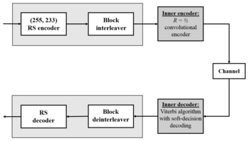
Deep-space concatenated coding system.[8] Notation: RS(255, 223) + CC («constraint length» = 7, code rate = 1/2).
One significant application of Reed–Solomon coding was to encode the digital pictures sent back by the Voyager program.
Voyager introduced Reed–Solomon coding concatenated with convolutional codes, a practice that has since become very widespread in deep space and satellite (e.g., direct digital broadcasting) communications.
Viterbi decoders tend to produce errors in short bursts. Correcting these burst errors is a job best done by short or simplified Reed–Solomon codes.
Modern versions of concatenated Reed–Solomon/Viterbi-decoded convolutional coding were and are used on the Mars Pathfinder, Galileo, Mars Exploration Rover and Cassini missions, where they perform within about 1–1.5 dB of the ultimate limit, the Shannon capacity.
These concatenated codes are now being replaced by more powerful turbo codes:
| Years | Code | Mission(s) |
|---|---|---|
| 1958–present | Uncoded | Explorer, Mariner, many others |
| 1968–1978 | convolutional codes (CC) (25, 1/2) | Pioneer, Venus |
| 1969–1975 | Reed-Muller code (32, 6) | Mariner, Viking |
| 1977–present | Binary Golay code | Voyager |
| 1977–present | RS(255, 223) + CC(7, 1/2) | Voyager, Galileo, many others |
| 1989–2003 | RS(255, 223) + CC(7, 1/3) | Voyager |
| 1989–2003 | RS(255, 223) + CC(14, 1/4) | Galileo |
| 1996–present | RS + CC (15, 1/6) | Cassini, Mars Pathfinder, others |
| 2004–present | Turbo codes[nb 1] | Messenger, Stereo, MRO, others |
| est. 2009 | LDPC codes | Constellation, MSL |
Constructions (encoding)[edit]
The Reed–Solomon code is actually a family of codes, where every code is characterised by three parameters: an alphabet size q, a block length n, and a message length k, with k < n ≤ q. The set of alphabet symbols is interpreted as the finite field of order q, and thus, q must be a prime power. In the most useful parameterizations of the Reed–Solomon code, the block length is usually some constant multiple of the message length, that is, the rate R = k/n is some constant, and furthermore, the block length is equal to or one less than the alphabet size, that is, n = q or n = q − 1.[citation needed]
Reed & Solomon’s original view: The codeword as a sequence of values[edit]
There are different encoding procedures for the Reed–Solomon code, and thus, there are different ways to describe the set of all codewords.
In the original view of Reed & Solomon (1960), every codeword of the Reed–Solomon code is a sequence of function values of a polynomial of degree less than k. In order to obtain a codeword of the Reed–Solomon code, the message symbols (each within the q-sized alphabet) are treated as the coefficients of a polynomial p of degree less than k, over the finite field F with q elements.
In turn, the polynomial p is evaluated at n ≤ q distinct points  of the field F, and the sequence of values is the corresponding codeword. Common choices for a set of evaluation points include {0, 1, 2, …, n − 1}, {0, 1, α, α2, …, αn−2}, or for n < q, {1, α, α2, …, αn−1}, … , where α is a primitive element of F.
Formally, the set  of codewords of the Reed–Solomon code is defined as follows:

Since any two distinct polynomials of degree less than  agree in at most
  points, this means that any two codewords of the Reed–Solomon code disagree in at least
  positions. Furthermore, there are two polynomials that do agree in points but are not equal, and thus, the distance of the Reed–Solomon code is exactly
  . Then the relative distance is
  , where
  is the rate. This trade-off between the relative distance and the rate is asymptotically optimal since, by the Singleton bound, every code satisfies
  .
.
Being a code that achieves this optimal trade-off, the Reed–Solomon code belongs to the class of maximum distance separable codes.
While the number of different polynomials of degree less than k and the number of different messages are both equal to  , and thus every message can be uniquely mapped to such a polynomial, there are different ways of doing this encoding. The original construction of Reed & Solomon (1960) interprets the message x as the coefficients of the polynomial p, whereas subsequent constructions interpret the message as the values of the polynomial at the first k points
  and obtain the polynomial p by interpolating these values with a polynomial of degree less than k. The latter encoding procedure, while being slightly less efficient, has the advantage that it gives rise to a systematic code, that is, the original message is always contained as a subsequence of the codeword.
Simple encoding procedure: The message as a sequence of coefficients[edit]
In the original construction of Reed & Solomon (1960), the message  is mapped to the polynomial
  with
with

The codeword of  is obtained by evaluating at
  different points of the field
  . Thus the classical encoding function
  for the Reed–Solomon code is defined as follows:

This function  is a linear mapping, that is, it satisfies
  for the following
  -matrix
  with elements from :

This matrix is the transpose of a Vandermonde matrix over . In other words, the Reed–Solomon code is a linear code, and in the classical encoding procedure, its generator matrix is .
Systematic encoding procedure: The message as an initial sequence of values[edit]
There is an alternative encoding procedure that also produces the Reed–Solomon code, but that does so in a systematic way. Here, the mapping from the message to the polynomial works differently: the polynomial is now defined as the unique polynomial of degree less than such that

To compute this polynomial from , one can use Lagrange interpolation.
Once it has been found, it is evaluated at the other points  of the field.
The alternative encoding function for the Reed–Solomon code is then again just the sequence of values:
Since the first entries of each codeword  coincide with , this encoding procedure is indeed systematic.
Since Lagrange interpolation is a linear transformation, is a linear mapping. In fact, we have  , where

Discrete Fourier transform and its inverse[edit]
A discrete Fourier transform is essentially the same as the encoding procedure; it uses the generator polynomial p(x) to map a set of evaluation points into the message values as shown above:
The inverse Fourier transform could be used to convert an error free set of n < q message values back into the encoding polynomial of k coefficients, with the constraint that in order for this to work, the set of evaluation points used to encode the message must be a set of increasing powers of α:


However, Lagrange interpolation performs the same conversion without the constraint on the set of evaluation points or the requirement of an error free set of message values and is used for systematic encoding, and in one of the steps of the Gao decoder.
The BCH view: The codeword as a sequence of coefficients[edit]
In this view, the message is interpreted as the coefficients of a polynomial  . The sender computes a related polynomial
  of degree
  where
where  and sends the polynomial . The polynomial is constructed by multiplying the message polynomial , which has degree , with a generator polynomial
  of degree
  that is known to both the sender and the receiver. The generator polynomial is defined as the polynomial whose roots are sequential powers of the Galois field primitive

For a «narrow sense code»,  .
.

Systematic encoding procedure[edit]
The encoding procedure for the BCH view of Reed–Solomon codes can be modified to yield a systematic encoding procedure, in which each codeword contains the message as a prefix, and simply appends error correcting symbols as a suffix. Here, instead of sending  , the encoder constructs the transmitted polynomial such that the coefficients of the largest monomials are equal to the corresponding coefficients of , and the lower-order coefficients of are chosen exactly in such a way that becomes divisible by . Then the coefficients of are a subsequence of the coefficients of . To get a code that is overall systematic, we construct the message polynomial by interpreting the message as the sequence of its coefficients.
Formally, the construction is done by multiplying by  to make room for the
  check symbols, dividing that product by to find the remainder, and then compensating for that remainder by subtracting it. The
  check symbols are created by computing the remainder
  :
:

The remainder has degree at most  , whereas the coefficients of
  in the polynomial
  are zero. Therefore, the following definition of the codeword has the property that the first coefficients are identical to the coefficients of :

As a result, the codewords are indeed elements of , that is, they are divisible by the generator polynomial :[10]

Properties[edit]
The Reed–Solomon code is a [n, k, n − k + 1] code; in other words, it is a linear block code of length n (over F) with dimension k and minimum Hamming distance  The Reed–Solomon code is optimal in the sense that the minimum distance has the maximum value possible for a linear code of size (n, k); this is known as the Singleton bound. Such a code is also called a maximum distance separable (MDS) code.
The error-correcting ability of a Reed–Solomon code is determined by its minimum distance, or equivalently, by , the measure of redundancy in the block. If the locations of the error symbols are not known in advance, then a Reed–Solomon code can correct up to  erroneous symbols, i.e., it can correct half as many errors as there are redundant symbols added to the block. Sometimes error locations are known in advance (e.g., «side information» in demodulator signal-to-noise ratios)—these are called erasures. A Reed–Solomon code (like any MDS code) is able to correct twice as many erasures as errors, and any combination of errors and erasures can be corrected as long as the relation 2E + S ≤ n − k is satisfied, where
  is the number of errors and
  is the number of erasures in the block.

Theoretical BER performance of the Reed-Solomon code (N=255, K=233, QPSK, AWGN). Step-like characteristic.
The theoretical error bound can be described via the following formula for the AWGN channel for FSK:[11]

and for other modulation schemes:

where  ,
,  ,
,  ,
,  is the symbol error rate in uncoded AWGN case and
  is the modulation order.
For practical uses of Reed–Solomon codes, it is common to use a finite field with  elements. In this case, each symbol can be represented as an
  -bit value.
The sender sends the data points as encoded blocks, and the number of symbols in the encoded block is  . Thus a Reed–Solomon code operating on 8-bit symbols has
  symbols per block. (This is a very popular value because of the prevalence of byte-oriented computer systems.) The number , with
  , of data symbols in the block is a design parameter. A commonly used code encodes
  eight-bit data symbols plus 32 eight-bit parity symbols in an
  -symbol block; this is denoted as a
  code, and is capable of correcting up to 16 symbol errors per block.
The Reed–Solomon code properties discussed above make them especially well-suited to applications where errors occur in bursts. This is because it does not matter to the code how many bits in a symbol are in error — if multiple bits in a symbol are corrupted it only counts as a single error. Conversely, if a data stream is not characterized by error bursts or drop-outs but by random single bit errors, a Reed–Solomon code is usually a poor choice compared to a binary code.
The Reed–Solomon code, like the convolutional code, is a transparent code. This means that if the channel symbols have been inverted somewhere along the line, the decoders will still operate. The result will be the inversion of the original data. However, the Reed–Solomon code loses its transparency when the code is shortened. The «missing» bits in a shortened code need to be filled by either zeros or ones, depending on whether the data is complemented or not. (To put it another way, if the symbols are inverted, then the zero-fill needs to be inverted to a one-fill.) For this reason it is mandatory that the sense of the data (i.e., true or complemented) be resolved before Reed–Solomon decoding.
Whether the Reed–Solomon code is cyclic or not depends on subtle details of the construction. In the original view of Reed and Solomon, where the codewords are the values of a polynomial, one can choose the sequence of evaluation points in such a way as to make the code cyclic. In particular, if is a primitive root of the field , then by definition all non-zero elements of take the form  for
for  , where
  . Each polynomial
  over gives rise to a codeword
  . Since the function
  is also a polynomial of the same degree, this function gives rise to a codeword
  ; since
  holds, this codeword is the cyclic left-shift of the original codeword derived from . So choosing a sequence of primitive root powers as the evaluation points makes the original view Reed–Solomon code cyclic. Reed–Solomon codes in the BCH view are always cyclic because BCH codes are cyclic.
[edit]
Designers are not required to use the «natural» sizes of Reed–Solomon code blocks. A technique known as «shortening» can produce a smaller code of any desired size from a larger code. For example, the widely used (255,223) code can be converted to a (160,128) code by padding the unused portion of the source block with 95 binary zeroes and not transmitting them. At the decoder, the same portion of the block is loaded locally with binary zeroes. The Delsarte–Goethals–Seidel[12] theorem illustrates an example of an application of shortened Reed–Solomon codes. In parallel to shortening, a technique known as puncturing allows omitting some of the encoded parity symbols.
BCH view decoders[edit]
The decoders described in this section use the BCH view of a codeword as a sequence of coefficients. They use a fixed generator polynomial known to both encoder and decoder.
Peterson–Gorenstein–Zierler decoder[edit]
Daniel Gorenstein and Neal Zierler developed a decoder that was described in a MIT Lincoln Laboratory report by Zierler in January 1960 and later in a paper in June 1961.[13] The Gorenstein–Zierler decoder and the related work on BCH codes are described in a book Error Correcting Codes by W. Wesley Peterson (1961).[14]
Formulation[edit]
The transmitted message,  , is viewed as the coefficients of a polynomial s(x):

As a result of the Reed-Solomon encoding procedure, s(x) is divisible by the generator polynomial g(x):

where α is a primitive element.
Since s(x) is a multiple of the generator g(x), it follows that it «inherits» all its roots.

Therefore,

The transmitted polynomial is corrupted in transit by an error polynomial e(x) to produce the received polynomial r(x).


Coefficient ei will be zero if there is no error at that power of x and nonzero if there is an error. If there are ν errors at distinct powers ik of x, then

The goal of the decoder is to find the number of errors (ν), the positions of the errors (ik), and the error values at those positions (eik). From those, e(x) can be calculated and subtracted from r(x) to get the originally sent message s(x).
Syndrome decoding[edit]
The decoder starts by evaluating the polynomial as received at points  . We call the results of that evaluation the «syndromes», Sj. They are defined as:

Note that  because has roots at
  , as shown in the previous section.
The advantage of looking at the syndromes is that the message polynomial drops out. In other words, the syndromes only relate to the error, and are unaffected by the actual contents of the message being transmitted. If the syndromes are all zero, the algorithm stops here and reports that the message was not corrupted in transit.
Error locators and error values[edit]
For convenience, define the error locators Xk and error values Yk as:

Then the syndromes can be written in terms of these error locators and error values as

This definition of the syndrome values is equivalent to the previous since  .
.
The syndromes give a system of n − k ≥ 2ν equations in 2ν unknowns, but that system of equations is nonlinear in the Xk and does not have an obvious solution. However, if the Xk were known (see below), then the syndrome equations provide a linear system of equations that can easily be solved for the Yk error values.

Consequently, the problem is finding the Xk, because then the leftmost matrix would be known, and both sides of the equation could be multiplied by its inverse, yielding Yk
In the variant of this algorithm where the locations of the errors are already known (when it is being used as an erasure code), this is the end. The error locations (Xk) are already known by some other method (for example, in an FM transmission, the sections where the bitstream was unclear or overcome with interference are probabilistically determinable from frequency analysis). In this scenario, up to errors can be corrected.
The rest of the algorithm serves to locate the errors, and will require syndrome values up to  , instead of just the
  used thus far. This is why 2x as many error correcting symbols need to be added as can be corrected without knowing their locations.
Error locator polynomial[edit]
There is a linear recurrence relation that gives rise to a system of linear equations. Solving those equations identifies those error locations Xk.
Define the error locator polynomial Λ(x) as

The zeros of Λ(x) are the reciprocals  . This follows from the above product notation construction since if
  then one of the multiplied terms will be zero
  , making the whole polynomial evaluate to zero.

Let  be any integer such that
  . Multiply both sides by
  and it will still be zero.
![{displaystyle {begin{aligned}&Y_{k}X_{k}^{j+nu }Lambda (X_{k}^{-1})=0.\[1ex]&Y_{k}X_{k}^{j+nu }left(1+Lambda _{1}X_{k}^{-1}+Lambda _{2}X_{k}^{-2}+cdots +Lambda _{nu }X_{k}^{-nu }right)=0.\[1ex]&Y_{k}X_{k}^{j+nu }+Lambda _{1}Y_{k}X_{k}^{j+nu }X_{k}^{-1}+Lambda _{2}Y_{k}X_{k}^{j+nu }X_{k}^{-2}+cdots +Lambda _{nu }Y_{k}X_{k}^{j+nu }X_{k}^{-nu }=0.\[1ex]&Y_{k}X_{k}^{j+nu }+Lambda _{1}Y_{k}X_{k}^{j+nu -1}+Lambda _{2}Y_{k}X_{k}^{j+nu -2}+cdots +Lambda _{nu }Y_{k}X_{k}^{j}=0.end{aligned}}}](https://wikimedia.org/api/rest_v1/media/math/render/svg/6573fa0f429ac4349f5da794df9c4fb7831e8cbf)
Sum for k = 1 to ν and it will still be zero.

Collect each term into its own sum.

Extract the constant values of  that are unaffected by the summation.

These summations are now equivalent to the syndrome values, which we know and can substitute in! This therefore reduces to

Subtracting  from both sides yields

Recall that j was chosen to be any integer between 1 and v inclusive, and this equivalence is true for any and all such values. Therefore, we have v linear equations, not just one. This system of linear equations can therefore be solved for the coefficients Λi of the error location polynomial:

The above assumes the decoder knows the number of errors ν, but that number has not been determined yet. The PGZ decoder does not determine ν directly but rather searches for it by trying successive values. The decoder first assumes the largest value for a trial ν and sets up the linear system for that value. If the equations can be solved (i.e., the matrix determinant is nonzero), then that trial value is the number of errors. If the linear system cannot be solved, then the trial ν is reduced by one and the next smaller system is examined. (Gill n.d., p. 35)
Find the roots of the error locator polynomial[edit]
Use the coefficients Λi found in the last step to build the error location polynomial. The roots of the error location polynomial can be found by exhaustive search. The error locators Xk are the reciprocals of those roots. The order of coefficients of the error location polynomial can be reversed, in which case the roots of that reversed polynomial are the error locators  (not their reciprocals ). Chien search is an efficient implementation of this step.
Calculate the error values[edit]
Once the error locators Xk are known, the error values can be determined. This can be done by direct solution for Yk in the error equations matrix given above, or using the Forney algorithm.
Calculate the error locations[edit]
Calculate ik by taking the log base of Xk. This is generally done using a precomputed lookup table.
Fix the errors[edit]
Finally, e(x) is generated from ik and eik and then is subtracted from r(x) to get the originally sent message s(x), with errors corrected.
Example[edit]
Consider the Reed–Solomon code defined in GF(929) with α = 3 and t = 4 (this is used in PDF417 barcodes) for a RS(7,3) code. The generator polynomial is

If the message polynomial is p(x) = 3 x2 + 2 x + 1, then a systematic codeword is encoded as follows.


Errors in transmission might cause this to be received instead.

The syndromes are calculated by evaluating r at powers of α.


Using Gaussian elimination:

Λ(x) = 329 x2 + 821 x + 001, with roots x1 = 757 = 3−3 and x2 = 562 = 3−4
The coefficients can be reversed to produce roots with positive exponents, but typically this isn’t used:
R(x) = 001 x2 + 821 x + 329, with roots 27 = 33 and 81 = 34
with the log of the roots corresponding to the error locations (right to left, location 0 is the last term in the codeword).
To calculate the error values, apply the Forney algorithm.
Ω(x) = S(x) Λ(x) mod x4 = 546 x + 732
Λ'(x) = 658 x + 821
e1 = −Ω(x1)/Λ'(x1) = 074
e2 = −Ω(x2)/Λ'(x2) = 122
Subtracting  from the received polynomial r(x) reproduces the original codeword s.
Berlekamp–Massey decoder[edit]
The Berlekamp–Massey algorithm is an alternate iterative procedure for finding the error locator polynomial. During each iteration, it calculates a discrepancy based on a current instance of Λ(x) with an assumed number of errors e:

and then adjusts Λ(x) and e so that a recalculated Δ would be zero. The article Berlekamp–Massey algorithm has a detailed description of the procedure. In the following example, C(x) is used to represent Λ(x).
Example[edit]
Using the same data as the Peterson Gorenstein Zierler example above:
| n | Sn+1 | d | C | B | b | m |
|---|---|---|---|---|---|---|
| 0 | 732 | 732 | 197 x + 1 | 1 | 732 | 1 |
| 1 | 637 | 846 | 173 x + 1 | 1 | 732 | 2 |
| 2 | 762 | 412 | 634 x2 + 173 x + 1 | 173 x + 1 | 412 | 1 |
| 3 | 925 | 576 | 329 x2 + 821 x + 1 | 173 x + 1 | 412 | 2 |
The final value of C is the error locator polynomial, Λ(x).
Euclidean decoder[edit]
Another iterative method for calculating both the error locator polynomial and the error value polynomial is based on Sugiyama’s adaptation of the extended Euclidean algorithm .
Define S(x), Λ(x), and Ω(x) for t syndromes and e errors:
![{displaystyle {begin{aligned}S(x)&=S_{t}x^{t-1}+S_{t-1}x^{t-2}+cdots +S_{2}x+S_{1}\[1ex]Lambda (x)&=Lambda _{e}x^{e}+Lambda _{e-1}x^{e-1}+cdots +Lambda _{1}x+1\[1ex]Omega (x)&=Omega _{e}x^{e}+Omega _{e-1}x^{e-1}+cdots +Omega _{1}x+Omega _{0}end{aligned}}}](https://wikimedia.org/api/rest_v1/media/math/render/svg/a84cd05dee4a72d23c59b3f95c4efdf3c8703600)
The key equation is:

For t = 6 and e = 3:

The middle terms are zero due to the relationship between Λ and syndromes.
The extended Euclidean algorithm can find a series of polynomials of the form
Ai(x) S(x) + Bi(x) xt = Ri(x)
where the degree of R decreases as i increases. Once the degree of Ri(x) < t/2, then
Ai(x) = Λ(x)
Bi(x) = −Q(x)
Ri(x) = Ω(x).
B(x) and Q(x) don’t need to be saved, so the algorithm becomes:
R−1 := xt
R0  := S(x)
A−1 := 0
A0  := 1
i := 0
while degree of Ri ≥ t/2
  i := i + 1
  Q := Ri-2 / Ri-1
  Ri := Ri-2 - Q Ri-1
  Ai := Ai-2 - Q Ai-1
to set low order term of Λ(x) to 1, divide Λ(x) and Ω(x) by Ai(0):
Λ(x) = Ai / Ai(0)
Ω(x) = Ri / Ai(0)
Ai(0) is the constant (low order) term of Ai.
Example[edit]
Using the same data as the Peterson–Gorenstein–Zierler example above:
| i | Ri | Ai |
|---|---|---|
| −1 | 001 x4 + 000 x3 + 000 x2 + 000 x + 000 | 000 |
| 0 | 925 x3 + 762 x2 + 637 x + 732 | 001 |
| 1 | 683 x2 + 676 x + 024 | 697 x + 396 |
| 2 | 673 x + 596 | 608 x2 + 704 x + 544 |
Λ(x) = A2 / 544 = 329 x2 + 821 x + 001
Ω(x) = R2 / 544 = 546 x + 732
Decoder using discrete Fourier transform[edit]
A discrete Fourier transform can be used for decoding.[15] To avoid conflict with syndrome names, let c(x) = s(x) the encoded codeword. r(x) and e(x) are the same as above. Define C(x), E(x), and R(x) as the discrete Fourier transforms of c(x), e(x), and r(x). Since r(x) = c(x) + e(x), and since a discrete Fourier transform is a linear operator, R(x) = C(x) + E(x).
Transform r(x) to R(x) using discrete Fourier transform. Since the calculation for a discrete Fourier transform is the same as the calculation for syndromes, t coefficients of R(x) and E(x) are the same as the syndromes:

Use  through
  as syndromes (they’re the same) and generate the error locator polynomial using the methods from any of the above decoders.
Let v = number of errors. Generate E(x) using the known coefficients  to
to  , the error locator polynomial, and these formulas

Then calculate C(x) = R(x) − E(x) and take the inverse transform (polynomial interpolation) of C(x) to produce c(x).
Decoding beyond the error-correction bound[edit]
The Singleton bound states that the minimum distance d of a linear block code of size (n,k) is upper-bounded by n − k + 1. The distance d was usually understood to limit the error-correction capability to ⌊(d−1) / 2⌋. The Reed–Solomon code achieves this bound with equality, and can thus correct up to ⌊(n−k) / 2⌋ errors. However, this error-correction bound is not exact.
In 1999, Madhu Sudan and Venkatesan Guruswami at MIT published «Improved Decoding of Reed–Solomon and Algebraic-Geometry Codes» introducing an algorithm that allowed for the correction of errors beyond half the minimum distance of the code.[16] It applies to Reed–Solomon codes and more generally to algebraic geometric codes. This algorithm produces a list of codewords (it is a list-decoding algorithm) and is based on interpolation and factorization of polynomials over  and its extensions.
Soft-decoding[edit]
The algebraic decoding methods described above are hard-decision methods, which means that for every symbol a hard decision is made about its value. For example, a decoder could associate with each symbol an additional value corresponding to the channel demodulator’s confidence in the correctness of the symbol. The advent of LDPC and turbo codes, which employ iterated soft-decision belief propagation decoding methods to achieve error-correction performance close to the theoretical limit, has spurred interest in applying soft-decision decoding to conventional algebraic codes. In 2003, Ralf Koetter and Alexander Vardy presented a polynomial-time soft-decision algebraic list-decoding algorithm for Reed–Solomon codes, which was based upon the work by Sudan and Guruswami.[17]
In 2016, Steven J. Franke and Joseph H. Taylor published a novel soft-decision decoder.[18]
MATLAB example[edit]
Encoder[edit]
Here we present a simple MATLAB implementation for an encoder.
function encoded = rsEncoder(msg, m, prim_poly, n, k)
    % RSENCODER Encode message with the Reed-Solomon algorithm
    % m is the number of bits per symbol
    % prim_poly: Primitive polynomial p(x). Ie for DM is 301
    % k is the size of the message
    % n is the total size (k+redundant)
    % Example: msg = uint8('Test')
    % enc_msg = rsEncoder(msg, 8, 301, 12, numel(msg));

    % Get the alpha
    alpha = gf(2, m, prim_poly);

    % Get the Reed-Solomon generating polynomial g(x)
    g_x = genpoly(k, n, alpha);

    % Multiply the information by X^(n-k), or just pad with zeros at the end to
    % get space to add the redundant information
    msg_padded = gf([msg zeros(1, n - k)], m, prim_poly);

    % Get the remainder of the division of the extended message by the
    % Reed-Solomon generating polynomial g(x)
    [~, remainder] = deconv(msg_padded, g_x);

    % Now return the message with the redundant information
    encoded = msg_padded - remainder;

end

% Find the Reed-Solomon generating polynomial g(x), by the way this is the
% same as the rsgenpoly function on matlab
function g = genpoly(k, n, alpha)
    g = 1;
    % A multiplication on the galois field is just a convolution
    for k = mod(1 : n - k, n)
        g = conv(g, [1 alpha .^ (k)]);
    end
end
Decoder[edit]
Now the decoding part:
function [decoded, error_pos, error_mag, g, S] = rsDecoder(encoded, m, prim_poly, n, k)
    % RSDECODER Decode a Reed-Solomon encoded message
    %   Example:
    % [dec, ~, ~, ~, ~] = rsDecoder(enc_msg, 8, 301, 12, numel(msg))
    max_errors = floor((n - k) / 2);
    orig_vals = encoded.x;
    % Initialize the error vector
    errors = zeros(1, n);
    g = [];
    S = [];

    % Get the alpha
    alpha = gf(2, m, prim_poly);

    % Find the syndromes (Check if dividing the message by the generator
    % polynomial the result is zero)
    Synd = polyval(encoded, alpha .^ (1:n - k));
    Syndromes = trim(Synd);

    % If all syndromes are zeros (perfectly divisible) there are no errors
    if isempty(Syndromes.x)
        decoded = orig_vals(1:k);
        error_pos = [];
        error_mag = [];
        g = [];
        S = Synd;
        return;
    end

    % Prepare for the euclidean algorithm (Used to find the error locating
    % polynomials)
    r0 = [1, zeros(1, 2 * max_errors)]; r0 = gf(r0, m, prim_poly); r0 = trim(r0);
    size_r0 = length(r0);
    r1 = Syndromes;
    f0 = gf([zeros(1, size_r0 - 1) 1], m, prim_poly);
    f1 = gf(zeros(1, size_r0), m, prim_poly);
    g0 = f1; g1 = f0;

    % Do the euclidean algorithm on the polynomials r0(x) and Syndromes(x) in
    % order to find the error locating polynomial
    while true
        % Do a long division
        [quotient, remainder] = deconv(r0, r1);
        % Add some zeros
        quotient = pad(quotient, length(g1));

        % Find quotient*g1 and pad
        c = conv(quotient, g1);
        c = trim(c);
        c = pad(c, length(g0));

        % Update g as g0-quotient*g1
        g = g0 - c;

        % Check if the degree of remainder(x) is less than max_errors
        if all(remainder(1:end - max_errors) == 0)
            break;
        end

        % Update r0, r1, g0, g1 and remove leading zeros
        r0 = trim(r1); r1 = trim(remainder);
        g0 = g1; g1 = g;
    end

    % Remove leading zeros
    g = trim(g);

    % Find the zeros of the error polynomial on this galois field
    evalPoly = polyval(g, alpha .^ (n - 1 : - 1 : 0));
    error_pos = gf(find(evalPoly == 0), m);

    % If no error position is found we return the received work, because
    % basically is nothing that we could do and we return the received message
    if isempty(error_pos)
        decoded = orig_vals(1:k);
        error_mag = [];
        return;
    end

    % Prepare a linear system to solve the error polynomial and find the error
    % magnitudes
    size_error = length(error_pos);
    Syndrome_Vals = Syndromes.x;
    b(:, 1) = Syndrome_Vals(1:size_error);
    for idx = 1 : size_error
        e = alpha .^ (idx * (n - error_pos.x));
        err = e.x;
        er(idx, :) = err;
    end

    % Solve the linear system
    error_mag = (gf(er, m, prim_poly)  gf(b, m, prim_poly))';
    % Put the error magnitude on the error vector
    errors(error_pos.x) = error_mag.x;
    % Bring this vector to the galois field
    errors_gf = gf(errors, m, prim_poly);

    % Now to fix the errors just add with the encoded code
    decoded_gf = encoded(1:k) + errors_gf(1:k);
    decoded = decoded_gf.x;

end

% Remove leading zeros from Galois array
function gt = trim(g)
    gx = g.x;
    gt = gf(gx(find(gx, 1) : end), g.m, g.prim_poly);
end

% Add leading zeros
function xpad = pad(x, k)
    len = length(x);
    if len < k
        xpad = [zeros(1, k - len) x];
    end
end
Reed Solomon original view decoders[edit]
The decoders described in this section use the Reed Solomon original view of a codeword as a sequence of polynomial values where the polynomial is based on the message to be encoded. The same set of fixed values are used by the encoder and decoder, and the decoder recovers the encoding polynomial (and optionally an error locating polynomial) from the received message.
Theoretical decoder[edit]
Reed & Solomon (1960) described a theoretical decoder that corrected errors by finding the most popular message polynomial. The decoder only knows the set of values  to
to  and which encoding method was used to generate the codeword’s sequence of values. The original message, the polynomial, and any errors are unknown. A decoding procedure could use a method like Lagrange interpolation on various subsets of n codeword values taken k at a time to repeatedly produce potential polynomials, until a sufficient number of matching polynomials are produced to reasonably eliminate any errors in the received codeword. Once a polynomial is determined, then any errors in the codeword can be corrected, by recalculating the corresponding codeword values. Unfortunately, in all but the simplest of cases, there are too many subsets, so the algorithm is impractical. The number of subsets is the binomial coefficient,
  , and the number of subsets is infeasible for even modest codes. For a
  code that can correct 3 errors, the naïve theoretical decoder would examine 359 billion subsets.
Berlekamp Welch decoder[edit]
In 1986, a decoder known as the Berlekamp–Welch algorithm was developed as a decoder that is able to recover the original message polynomial as well as an error «locator» polynomial that produces zeroes for the input values that correspond to errors, with time complexity  , where is the number of values in a message. The recovered polynomial is then used to recover (recalculate as needed) the original message.
Example[edit]
Using RS(7,3), GF(929), and the set of evaluation points ai = i − 1
a = {0, 1, 2, 3, 4, 5, 6}
If the message polynomial is
p(x) = 003 x2 + 002 x + 001
The codeword is
c = {001, 006, 017, 034, 057, 086, 121}
Errors in transmission might cause this to be received instead.
b = c + e = {001, 006, 123, 456, 057, 086, 121}
The key equations are:

Assume maximum number of errors: e = 2. The key equations become:


Using Gaussian elimination:

Q(x) = 003 x4 + 916 x3 + 009 x2 + 007 x + 006
E(x) = 001 x2 + 924 x + 006
Q(x) / E(x) = P(x) = 003 x2 + 002 x + 001
Recalculate P(x) where E(x) = 0 : {2, 3} to correct b resulting in the corrected codeword:
c = {001, 006, 017, 034, 057, 086, 121}
Gao decoder[edit]
In 2002, an improved decoder was developed by Shuhong Gao, based on the extended Euclid algorithm.[6]
Example[edit]
Using the same data as the Berlekamp Welch example above:
| i | Ri | Ai |
|---|---|---|
| −1 | 001 x7 + 908 x6 + 175 x5 + 194 x4 + 695 x3 + 094 x2 + 720 x + 000 | 000 |
| 0 | 055 x6 + 440 x5 + 497 x4 + 904 x3 + 424 x2 + 472 x + 001 | 001 |
| 1 | 702 x5 + 845 x4 + 691 x3 + 461 x2 + 327 x + 237 | 152 x + 237 |
| 2 | 266 x4 + 086 x3 + 798 x2 + 311 x + 532 | 708 x2 + 176 x + 532 |
Q(x) = R2 = 266 x4 + 086 x3 + 798 x2 + 311 x + 532
E(x) = A2 = 708 x2 + 176 x + 532
divide Q(x) and E(x) by most significant coefficient of E(x) = 708. (Optional)
Q(x) = 003 x4 + 916 x3 + 009 x2 + 007 x + 006
E(x) = 001 x2 + 924 x + 006
Q(x) / E(x) = P(x) = 003 x2 + 002 x + 001
Recalculate P(x) where E(x) = 0 : {2, 3} to correct b resulting in the corrected codeword:
c = {001, 006, 017, 034, 057, 086, 121}
See also[edit]
- BCH code
- Cyclic code
- Chien search
- Berlekamp–Massey algorithm
- Forward error correction
- Berlekamp–Welch algorithm
- Folded Reed–Solomon code
Notes[edit]
- ^ Authors in Andrews et al. (2007), provide simulation results which show that for the same code rate (1/6) turbo codes outperform Reed-Solomon concatenated codes up to 2 dB (bit error rate).[9]
References[edit]
- ^ Reed & Solomon (1960)
- ^ D. Gorenstein and N. Zierler, «A class of cyclic linear error-correcting codes in p^m symbols», J. SIAM, vol. 9, pp. 207–214, June 1961
- ^ Error Correcting Codes by W_Wesley_Peterson, 1961
- ^ Error Correcting Codes by W_Wesley_Peterson, second edition, 1972
- ^ Yasuo Sugiyama, Masao Kasahara, Shigeichi Hirasawa, and Toshihiko Namekawa. A method for solving key equation for decoding Goppa codes. Information and Control, 27:87–99, 1975.
- ^ a b Gao, Shuhong (January 2002), New Algorithm For Decoding Reed-Solomon Codes (PDF), Clemson
- ^ Immink, K. A. S. (1994), «Reed–Solomon Codes and the Compact Disc», in Wicker, Stephen B.; Bhargava, Vijay K. (eds.), Reed–Solomon Codes and Their Applications, IEEE Press, ISBN 978-0-7803-1025-4
- ^ J. Hagenauer, E. Offer, and L. Papke, Reed Solomon Codes and Their Applications. New York IEEE Press, 1994 — p. 433
- ^ a b Andrews, Kenneth S., et al. «The development of turbo and LDPC codes for deep-space applications.» Proceedings of the IEEE 95.11 (2007): 2142-2156.
- ^ See Lin & Costello (1983, p. 171), for example.
- ^ «Analytical Expressions Used in bercoding and BERTool». Archived from the original on 2019-02-01. Retrieved 2019-02-01.
- ^ Pfender, Florian; Ziegler, Günter M. (September 2004), «Kissing Numbers, Sphere Packings, and Some Unexpected Proofs» (PDF), Notices of the American Mathematical Society, 51 (8): 873–883, archived (PDF) from the original on 2008-05-09, retrieved 2009-09-28. Explains the Delsarte-Goethals-Seidel theorem as used in the context of the error correcting code for compact disc.
- ^ D. Gorenstein and N. Zierler, «A class of cyclic linear error-correcting codes in p^m symbols,» J. SIAM, vol. 9, pp. 207–214, June 1961
- ^ Error Correcting Codes by W Wesley Peterson, 1961
- ^ Shu Lin and Daniel J. Costello Jr, «Error Control Coding» second edition, pp. 255–262, 1982, 2004
- ^ Guruswami, V.; Sudan, M. (September 1999), «Improved decoding of Reed–Solomon codes and algebraic geometry codes», IEEE Transactions on Information Theory, 45 (6): 1757–1767, CiteSeerX 10.1.1.115.292, doi:10.1109/18.782097
- ^ Koetter, Ralf; Vardy, Alexander (2003). «Algebraic soft-decision decoding of Reed–Solomon codes». IEEE Transactions on Information Theory. 49 (11): 2809–2825. CiteSeerX 10.1.1.13.2021. doi:10.1109/TIT.2003.819332.
- ^ Franke, Steven J.; Taylor, Joseph H. (2016). «Open Source Soft-Decision Decoder for the JT65 (63,12) Reed–Solomon Code» (PDF). QEX (May/June): 8–17. Archived (PDF) from the original on 2017-03-09. Retrieved 2017-06-07.
Further reading[edit]
- Gill, John (n.d.), EE387 Notes #7, Handout #28 (PDF), Stanford University, archived from the original (PDF) on June 30, 2014, retrieved April 21, 2010
- Hong, Jonathan; Vetterli, Martin (August 1995), «Simple Algorithms for BCH Decoding» (PDF), IEEE Transactions on Communications, 43 (8): 2324–2333, doi:10.1109/26.403765
- Lin, Shu; Costello, Jr., Daniel J. (1983), Error Control Coding: Fundamentals and Applications, New Jersey, NJ: Prentice-Hall, ISBN 978-0-13-283796-5
- Massey, J. L. (1969), «Shift-register synthesis and BCH decoding» (PDF), IEEE Transactions on Information Theory, IT-15 (1): 122–127, doi:10.1109/tit.1969.1054260
- Peterson, Wesley W. (1960), «Encoding and Error Correction Procedures for the Bose-Chaudhuri Codes», IRE Transactions on Information Theory, IT-6 (4): 459–470, doi:10.1109/TIT.1960.1057586
- Reed, Irving S.; Solomon, Gustave (1960), «Polynomial Codes over Certain Finite Fields», Journal of the Society for Industrial and Applied Mathematics, 8 (2): 300–304, doi:10.1137/0108018
- Welch, L. R. (1997), The Original View of Reed–Solomon Codes (PDF), Lecture Notes
- Berlekamp, Elwyn R. (1967), Nonbinary BCH decoding, International Symposium on Information Theory, San Remo, Italy
- Berlekamp, Elwyn R. (1984) [1968], Algebraic Coding Theory (Revised ed.), Laguna Hills, CA: Aegean Park Press, ISBN 978-0-89412-063-3
- Cipra, Barry Arthur (1993), «The Ubiquitous Reed–Solomon Codes», SIAM News, 26 (1)
- Forney, Jr., G. (October 1965), «On Decoding BCH Codes», IEEE Transactions on Information Theory, 11 (4): 549–557, doi:10.1109/TIT.1965.1053825
- Koetter, Ralf (2005), Reed–Solomon Codes, MIT Lecture Notes 6.451 (Video), archived from the original on 2013-03-13
- MacWilliams, F. J.; Sloane, N. J. A. (1977), The Theory of Error-Correcting Codes, New York, NY: North-Holland Publishing Company
- Reed, Irving S.; Chen, Xuemin (1999), Error-Control Coding for Data Networks, Boston, MA: Kluwer Academic Publishers
External links[edit]
Information and tutorials[edit]
- Introduction to Reed–Solomon codes: principles, architecture and implementation (CMU)
- A Tutorial on Reed–Solomon Coding for Fault-Tolerance in RAID-like Systems
- Algebraic soft-decoding of Reed–Solomon codes
- Wikiversity:Reed–Solomon codes for coders
- BBC R&D White Paper WHP031
- Geisel, William A. (August 1990), Tutorial on Reed–Solomon Error Correction Coding, Technical Memorandum, NASA, TM-102162
- Concatenated codes by Dr. Dave Forney (scholarpedia.org).
- Reid, Jeff A. (April 1995), CRC and Reed Solomon ECC (PDF)
Implementations[edit]
- FEC library in C by Phil Karn (aka KA9Q) includes Reed–Solomon codec, both arbitrary and optimized (223,255) version
- Schifra Open Source C++ Reed–Solomon Codec
- Henry Minsky’s RSCode library, Reed–Solomon encoder/decoder
- Open Source C++ Reed–Solomon Soft Decoding library
- Matlab implementation of errors and-erasures Reed–Solomon decoding
- Octave implementation in communications package
- Pure-Python implementation of a Reed–Solomon codec
4.2. Введение в коды Рида-Соломона: принципы, архитектура и реализация
Коды Рида-Соломона были предложены в 1960 году Ирвином Ридом (Irving S. Reed) и Густавом Соломоном (Gustave Solomon), являвшимися сотрудниками Линкольнской лаборатории МТИ. Ключом к использованию этой технологии стало изобретение эффективного алгоритма декодирования Элвином Беликамфом (Elwyn Berlekamp; http://en.wikipedia.org/wiki/Berlekamp-Massey_algorithm), профессором Калифорнийского университета (Беркли). Коды Рида-Соломона (см. также http://www.4i2i.com/reed_solomon_codes.htm) базируются на блочном принципе коррекции ошибок и используются в огромном числе приложений в сфере цифровых телекоммуникаций и при построении запоминающих устройств. Коды Рида-Соломона применяются для исправления ошибок во многих системах:
- устройствах памяти (включая магнитные ленты, CD, DVD, штриховые коды, и т.д.);
- беспроводных или мобильных коммуникациях (включая сотовые телефоны, микроволновые каналы и т.д.);
- спутниковых коммуникациях;
- цифровом телевидении / DVB (digital video broadcast);
- скоростных модемах, таких как ADSL, xDSL и т.д.
На
рис.
4.3 показаны практические приложения (дальние космические проекты) коррекции ошибок с использованием различных алгоритмов (Хэмминга, кодов свертки, Рида-Соломона и пр.). Данные и сам рисунок взяты из http://en.wikipedia.org/wiki/Reed-Solomon_error_correction.
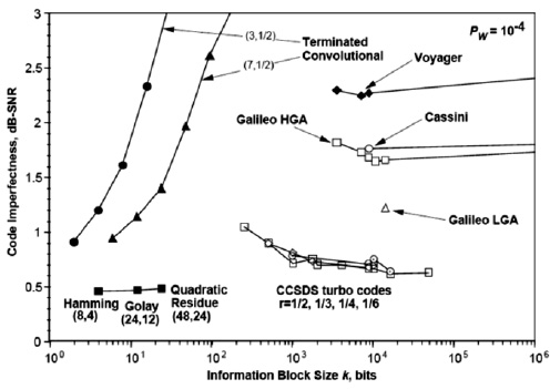
Рис.
4.3.
Несовершенство кода, как функция размера информационного блока для разных задач и алгоритмов
Типовая система представлена ниже (см. http://www.4i2i.com/reed_solomon_codes.htm)
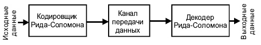
Рис.
4.4.
Схема коррекции ошибок Рида-Соломона
Кодировщик Рида-Соломона берет блок цифровых данных и добавляет дополнительные «избыточные» биты. Ошибки происходят при передаче по каналам связи или по разным причинам при запоминании (например, из-за шума или наводок, царапин на CD и т.д.). Декодер Рида-Соломона обрабатывает каждый блок, пытается исправить ошибки и восстановить исходные данные. Число и типы ошибок, которые могут быть исправлены, зависят от характеристик кода Рида-Соломона.
Свойства кодов Рида-Соломона
Коды Рида-Соломона являются субнабором кодов BCH и представляют собой линейные блочные коды. Код Рида-Соломона специфицируются как RS(n,k) s -битных символов.
Это означает, что кодировщик воспринимает k информационных символов по s битов каждый и добавляет символы четности для формирования n символьного кодового слова. Имеется nk символов четности по s битов каждый. Декодер Рида-Соломона может корректировать до t символов, которые содержат ошибки в кодовом слове, где 2t = n–k.
Диаграмма, представленная ниже, показывает типовое кодовое слово Рида-Соломона:
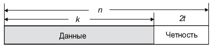
Рис.
4.5.
Структура кодового слова R-S
Пример. Популярным кодом Рида-Соломона является RS(255, 223) с 8-битными символами. Каждое кодовое слово содержит 255 байт, из которых 223 являются информационными и 32 байтами четности. Для этого кода
n = 255, k = 223, s = 8
2t = 32, t = 16
Декодер может исправить любые 16 символов с ошибками в кодовом слове: то есть ошибки могут быть исправлены, если число искаженных байт не превышает 16.
При размере символа s, максимальная длина кодового слова ( n ) для кода Рида-Соломона равна n = 2s – 1.
Например, максимальная длина кода с 8-битными символами ( s = 8 ) равна 255 байтам.
Коды Рида-Соломона могут быть в принципе укорочены путем обнуления некоторого числа информационных символов на входе кодировщика (передавать их в этом случае не нужно). При передаче данных декодеру эти нули снова вводятся в массив.
Пример. Код (255, 223), описанный выше, может быть укорочен до (200, 168). Кодировщик будет работать с блоком данных 168 байт, добавит 55 нулевых байт, сформирует кодовое слово (255, 223) и передаст только 168 информационных байт и 32 байта четности.
Объем вычислительной мощности, необходимой для кодирования и декодирования кодов Рида-Соломона, зависит от числа символов четности. Большое значение t означает, что большее число ошибок может быть исправлено, но это потребует большей вычислительной мощности по сравнению с вариантом при меньшем t.
Ошибки в символах
Одна ошибка в символе происходит, когда 1 бит символа оказывается неверным или когда все биты неверны.
Пример. Код RS(255,223) может исправить до 16 ошибок в символах. В худшем случае, могут иметь место 16 битовых ошибок в разных символах (байтах). В лучшем случае, корректируются 16 полностью неверных байт, при этом исправляется 16 x 8 = 128 битовых ошибок.
Коды Рида-Соломона особенно хорошо подходят для корректировки кластеров ошибок (когда неверными оказываются большие группы бит кодового слова, следующие подряд).
Декодирование
Алгебраические процедуры декодирования Рида-Соломона могут исправлять ошибки и потери. Потерей считается случай, когда положение неверного символа известно. Декодер может исправить до t ошибок или до 2t потерь. Данные о потере (стирании) могут быть получены от демодулятора цифровой коммуникационной системы, т.е. демодулятор помечает полученные символы, которые вероятно содержат ошибки.
Когда кодовое слово декодируется, возможны три варианта.
- Если 2s + r < 2t ( s ошибок, r потерь), тогда исходное переданное кодовое слово всегда будет восстановлено. В противном случае
- Декодер детектирует ситуацию, когда он не может восстановить исходное кодовое слово. или
- Декодер некорректно декодирует и неверно восстановит кодовое слово без какого-либо указания на этот факт.
Вероятность каждого из этих вариантов зависит от типа используемого кода Рида-Соломона, а также от числа и распределения ошибок.
Last time, we talked about error correction and detection, covering some basics like Hamming distance, CRCs, and Hamming codes. If you are new to this topic, I would strongly suggest going back to read that article before this one.
This time we are going to cover Reed-Solomon codes. (I had meant to cover this topic in Part XV, but the article was getting to be too long, so I’ve split it roughly in half.) These are one of the workhorses of error-correction, and they are used in overwhelming abundance to correct short bursts of errors. We’ll see that encoding a message using Reed-Solomon is fairly simple, so easy that we can even do it in C on an embedded system.
We’re also going to talk about some performance metrics of error-correcting codes.
Reed-Solomon Codes
Reed-Solomon codes, like many other error-correcting codes, are parameterized. A Reed-Solomon ( (n,k) ) code, where ( n=2^m-1 ) and ( k=n-2t ), can correct up to ( t ) errors. They are not binary codes; each symbol must have ( 2^m ) possible values, and is typically an element of ( GF(2^m) ).
The Reed-Solomon codes with ( n=255 ) are very common, since then each symbol is an element of ( GF(2^8) ) and can be represented as a single byte. A ( (255, 247) ) RS code would be able to correct 4 errors, and a ( (255,223) ) RS code would be able to correct 16 errors, with each error being an arbitrary error in one transmitted symbol.
You may have noticed a pattern in some of the coding techniques discussed in the previous article:
- If we compute the parity of a string of bits, and concatenate a parity bit, the resulting message has a parity of zero modulo 2
- If we compute the checksum of a string of bytes, and concatenate a negated checksum, the resulting message has a checksum of zero modulo 256
- If we compute the CRC of a message (with no initial/final bit flips), and concatenate the CRC, the resulting message has a remainder of zero modulo the CRC polynomial
- If we compute parity bits of a Hamming code, and concatenate them to the data bits, the resulting message has a remainder of zero modulo the Hamming code polynomial
In all cases, we have this magic technique of taking data bits, using a division algorithm to compute the remainder, and concatenating the remainder, such that the resulting message has zero remainder. If we receive a message which does have a nonzero remainder, we can detect this, and in some cases use the nonzero remainder to determine where the errors occurred and correct them.
Parity and checksum are poor methods because they are unable to detect transpositions. It’s easy to cancel out a parity flip; it’s much harder to cancel out a CRC error by accidentally flipping another bit elsewhere.
What if there was an encoding algorithm that was somewhat similar to a checksum, in that it operated on a byte-by-byte basis, but had robustness to swapped bytes? Reed-Solomon is such an algorithm. And it amounts to doing the same thing as all the other linear coding techniques we’ve talked about to encode a message:
- take data bits
- use a polynomial division algorithm to compute a remainder
- create a codeword by concatenating the data bits and the remainder bits
- a valid codeword now has a zero remainder
In this article, I am going to describe Reed-Solomon encoding, but not the typical decoding methods, which are somewhat complicated, and include fancy-sounding steps like the Berlekamp-Massey algorithm (yes, this is the same one we saw in part VI, only it’s done in ( GF(2^m) ) instead of the binary ( GF(2) ) version), the Chien search, and the Forney algorithm. If you want to learn more, I would recommend reading the BBC white paper WHP031, in the list of references, which does go into just the right level of detail, and has lots of examples.
In addition to being more complicated to understand, decoding is also more computationally intensive. Reed-Solomon encoders are straightforward to implement in hardware — which we’ll see a bit later — and are simple to implement in software in an embedded system. Decoders are trickier, and you’d probably want something more powerful than an 8-bit microcontroller to execute them, or they’ll be very slow. The first use of Reed-Solomon in space communications was on the Voyager missions, where an encoder was included without certainty that the received signals could be decoded back on earth. From a NASA Tutorial on Reed-Solomon Error Correction Coding by William A. Geisel:
The Reed-Solomon (RS) codes have been finding widespread
applications ever since the 1977 Voyager’s deep space
communications system. At the time of Voyager’s launch, efficient
encoders existed, but accurate decoding methods were not even
available! The Jet Propulsion Laboratory (JPL) scientists and
engineers gambled that by the time Voyager II would reach Uranus in
1986, decoding algorithms and equipment would be both available and
perfected. They were correct! Voyager’s communications system was
able to obtain a data rate of 21,600 bits per second from
2 billion miles away with a received signal energy 100 billion
times weaker than a common wrist watch battery!
The statement “accurate decoding methods were not even available” in 1977 is a bit suspicious, although this general idea of faith-that-a-decoder-could-be-constructed is in several other accounts:
Lahmeyer, the sole engineer on the project, and his team of technicians and builders worked tirelessly to get the decoder working by the time Voyager reached Uranus. Otherwise, they would have had to slow down the rate of data received to decrease noise interference. “Each chip had to be hand wired,” Lahmeyer says. “Thankfully, we got it working on time.”
(Jefferson City Magazine, June 2015)
In order to make the extended mission to Uranus and Neptune possible,
some new and never-before-tried technologies had to be designed into
the spacecraft and novel new techniques for using the hardware to its
fullest had to be validated for use. One notable requirement was the need
to improve error correction coding of the data stream over the very inefficient method which had been used for all previous missions (and for
the Voyagers at Jupiter and Saturn), because the much lower maximum
data rates from Uranus and Neptune (due to distance) would have greatly
compromised the number of pictures and other data that could have been
obtained. A then-new and highly efficient data coding method called
Reed-Solomon (RS) coding was planned for Voyager at Uranus, and the
coding device was integrated into the spacecraft design. The problem
was that although RS coding is easy to do and the encoding device was
relatively simple to make, decoding the data after receipt on the ground
is so mathematically intensive that no computer on Earth was able to
handle the decoding task at the time Voyager was designed – or even
launched. The increase of data throughput using the RS coder was about
a factor of three over the old, standard Golay coding, so including the
capability was considered highly worthwhile. It was assumed that a decoder could be developed by the time Voyager needed it at Uranus. Such
was the case, and today RS coding is routinely used in CD players and
many other common household electronic devices.
(Sirius Astronomer, August 2017)
Geisel probably meant “efficient” rather than “accurate”; decoding algorithms were well-known before a NASA report in 1978 which states
These codes were first described
by I. S. Reed and G. Solomon in 1960. A systematic decoding algorithm was not
discovered until 1968 by E. Berlekamp. Because of their complexity, the RS
codes are not widely used except when no other codes are suitable.
Details of Reed-Solomon Encoding
At any rate, with Reed-Solomon, we have a polynomial, but instead of the coefficients being 0 or 1 like our usual polynomials in ( GF(2)[x] ), this time the coefficients are elements of ( GF(2^m) ). A byte-oriented Reed-Solomon encoding uses ( GF(2^8) ). The polynomial used in Reed-Solomon is usually written as ( g(x) ), the generator polynomial, with
$$g(x) = (x+lambda^b)(x+lambda^{b+1})(x+lambda^{b+2})ldots (x+lambda^{b+n-k-1})$$
where ( lambda ) is a primitive element of ( GF(2^m) ) and ( b ) is some constant, usually 0 or 1 or ( -t ). This means the polynomial’s roots are successive powers of ( lambda ), and that makes the math work out just fine.
All we do is treat the message as a polynomial ( M(x) ), calculate a remainder ( r(x) = x^{n-k} M(x) bmod g(x) ), and then concatenate it to the message; the resulting codeword ( C(x) = x^{n-k}M(x) + r(x) ), is guaranteed to be a multiple of the generator polynomial ( g(x) ). At the receiving end, we calculate ( C(x) bmod g(x) ) and if it’s zero, everything’s great; otherwise we have to do some gory math, but this allows us to find and correct errors in up to ( t ) symbols.
That probably sounds rather abstract, so let’s work through an example.
Reed-Solomon in Python
We’re going to encode some messages using Reed-Solomon in two ways, first using the unireedsolomon library, and then from scratch using libgf2. If you’re going to use a library, you’ll need to be really careful; the library should be universal, meaning you can encode or decode any particular flavor of Reed-Solomon — like the CRC, there are many possible variants, and you need to be able to specify the polynomial of the Galois field used for each symbol, along with the generator element ( lambda ) and the initial power ( b ). If anyone tells you they’re using the Reed-Solomon ( (255,223) ) code, they’re smoking something funny, because there’s more than one, and you need to know which particular variant in order to communicate properly.
There are two examples in the BBC white paper:
- one using ( RS(15,11) ) for 4-bit symbols, with symbol field ( GF(2)[y]/(y^4 + y + 1) ); for the generator, ( lambda = y = {tt 2} ) and ( b=0 ), forming the generator polynomial
$$begin{align}
g(x) &= (x+1)(x+lambda)(x+lambda^2)(x+lambda^3) cr
&= x^4 + lambda^{12}x^3 + lambda^{4}x^2 + x + lambda^6 cr
&= x^4 + 15x^3 + 3x^2 + x + 12 cr
&= x^4 + {tt F} x^3 + {tt 3}x^2 + {tt 1}x + {tt 12}
end{align}$$
- another using the DVB-T specification that uses ( RS(255,239) ) for 8-bit symbols, with symbol field ( GF(2)[y]/(y^8 + y^4 + y^3 + y^2 + 1) ) (hex representation
11d) and for the generator, ( lambda = y = {tt 2} ) and ( b=0 ), forming the generator polynomial
$$begin{align}
g(x) &= (x+1)(x+lambda)(x+lambda^2)(x+lambda^3)ldots(x+lambda^{15}) cr
&= x^{16} + lambda^{12}x^3 + lambda^{4}x^2 + x + lambda^6 cr
&= x^{16} + 59x^{15} + 13x^{14} + 104x^{13} + 189x^{12} + 68x^{11} + 209x^{10} + 30x^9 + 8x^8 cr
&qquad + 163x^7 + 65x^6 + 41x^5 + 229x^4 + 98x^3 + 50x^2 + 36x + 59 cr
&= x^{16} + {tt 3B} x^{15} + {tt 0D}x^{14} + {tt 68}x^{13} + {tt BD}x^{12} + {tt 44}x^{11} + {tt d1}x^{10} + {tt 1e}x^9 + {tt 08}x^8cr
&qquad + {tt A3}x^7 + {tt 41}x^6 + {tt 29}x^5 + {tt E5}x^4 + {tt 62}x^3 + {tt 32}x^2 + {tt 24}x + {tt 3B}
end{align}$$
In unireedsolomon, the RSCoder class is used, with these parameters:
c_exp— this is the number of bits per symbol, 4 and 8 for our two examplesprim— this is the symbol field polynomial, 0x13 and 0x11d for our two examplesgenerator— this is the generator element in the symbol field, 0x2 for both examplesfcr— this is the “first consecutive root” ( b ), with ( b=0 ) for both examples
You can verify the generator polynomial by encoding the message ( M(x) = 1 ), all zero symbols with a trailing one symbol at the end; this will create a codeword ( C(x) = x^{n-k} + r(x) = g(x) ).
Let’s do it!
import unireedsolomon as rs

def codeword_symbols(msg):
    return [ord(c) for c in msg]

def find_generator(rscoder):
    """ Returns the generator polynomial of an RSCoder class """
    msg = [0]*(rscoder.k - 1) + [1]
    degree = rscoder.n - rscoder.k
    codeword = rscoder.encode(msg)
    # look at the trailing elements of the codeword
    return codeword_symbols(codeword[(-degree-1):])

rs4 = rs.RSCoder(15,11,generator=2,prim=0x13,fcr=0,c_exp=4)
print "g4(x) = %s" % find_generator(rs4)

rs8 = rs.RSCoder(255,239,generator=2,prim=0x11d,fcr=0,c_exp=8)
print "g8(x) = %s" % find_generator(rs8)
g4(x) = [1, 15, 3, 1, 12]
g8(x) = [1, 59, 13, 104, 189, 68, 209, 30, 8, 163, 65, 41, 229, 98, 50, 36, 59]
Easy as pie!
Encoding messages is just a matter of using either a string (byte array) or a list of message symbols, and we get a string back by default. (You can use encode(msg, return_string=False) but then you get a bunch of GF2Int objects back rather than integer coefficients.)
(Warning: the unireedsolomon package uses a global singleton to manage Galois field arithmetic, so if you want to have multiple RSCoder objects out there, they’ll only work if they share the same field generator polynomial. This is why each time I want to switch back between the 4-bit and the 8-bit RSCoder, I have to create a new object, so that it reconfigures the way Galois field arithmetic works.)
The BBC white paper has a sample encoding only for the 4-bit ( RS(15,11) ) example, using ( [1,2,3,4,5,6,7,8,9,10,11] ) which produces remainder ( [3,3,12,12] ):
rs4 = rs.RSCoder(15,11,generator=2,prim=0x13,fcr=0,c_exp=4)
encmsg15 = codeword_symbols(rs4.encode([1,2,3,4,5,6,7,8,9,10,11]))
print "RS(15,11) encoded example message from BBC WHP031:n", encmsg15
RS(15,11) encoded example message from BBC WHP031:
[1, 2, 3, 4, 5, 6, 7, 8, 9, 10, 11, 3, 3, 12, 12]
The real fun begins when we can start encoding actual messages, like Ernie, you have a banana in your ear! Since this has length 37, let’s use a shortened version of the code, ( RS(53,37) ).
Mama’s Little Baby Loves Shortnin’, Shortnin’, Mama’s Little Baby Loves Shortnin’ Bread
Oh, we haven’t talked about shortened codes yet — this is where we just omit the initial symbols in a codeword, and both transmitter and receiver agree treat them as implied zeros. An eight-bit ( RS(53,37) ) transmitter encodes as codeword polynomials of degree 52, and the receiver just zero-extends them to degree 254 (with 202 implied zero bytes added at the beginning) for the purposes of decoding just like any other ( RS(255,239) ) code.
rs8s = rs.RSCoder(53,37,generator=2,prim=0x11d,fcr=0,c_exp=8)
msg = 'Ernie, you have a banana in your ear!'
codeword = rs8s.encode(msg)
print ('codeword=%r' % codeword)
remainder = codeword[-16:]
print ('remainder(hex) = %s' % remainder.encode('hex'))
codeword='Ernie, you have a banana in your ear!U,xa3xb4dx00:Rxc4Px11xf4nx0fxeax9b'
remainder(hex) = 552ca3b464003a52c45011f46e0fea9b
That binary stuff after the message is the remainder. Now we can decode all sorts of messages with errors:
for init_msg in [
    'Ernie, you have a banana in your ear!',
    'Billy! You have a banana in your ear!',
    'Arnie! You have a potato in your ear!',
    'Eddie? You hate a banana in your car?',
    '01234567ou have a banana in your ear!',
    '012345678u have a banana in your ear!',
]:
    decoded_msg, decoded_remainder = rs8s.decode(init_msg+remainder)
    print "%s -> %s" % (init_msg, decoded_msg)
Ernie, you have a banana in your ear! -> Ernie, you have a banana in your ear!
Billy! You have a banana in your ear! -> Ernie, you have a banana in your ear!
Arnie! You have a potato in your ear! -> Ernie, you have a banana in your ear!
Eddie? You hate a banana in your car? -> Ernie, you have a banana in your ear!
01234567ou have a banana in your ear! -> Ernie, you have a banana in your ear!
---------------------------------------------------------------------------
RSCodecError                              Traceback (most recent call last)
 in ()
      7     '012345678u have a banana in your ear!',
      8 ]:
----> 9     decoded_msg, decoded_remainder = rs8s.decode(init_msg+remainder)
     10     print "%s -> %s" % (init_msg, decoded_msg)

/Users/jmsachs/anaconda/lib/python2.7/site-packages/unireedsolomon/rs.pyc in decode(self, r, nostrip, k, erasures_pos, only_erasures, return_string)
    321         # being the rightmost byte
    322         # X is a corresponding array of GF(2^8) values where X_i = alpha^(j_i)
--> 323         X, j = self._chien_search(sigma)
    324
    325         # Sanity check: Cannot guarantee correct decoding of more than n-k errata (Singleton Bound, n-k being the minimum distance), and we cannot even check if it's correct (the syndrome will always be all 0 if we try to decode above the bound), thus it's better to just return the input as-is.

/Users/jmsachs/anaconda/lib/python2.7/site-packages/unireedsolomon/rs.pyc in _chien_search(self, sigma)
    822         errs_nb = len(sigma) - 1 # compute the exact number of errors/errata that this error locator should find
    823         if len(j) != errs_nb:
--> 824             raise RSCodecError("Too many (or few) errors found by Chien Search for the errata locator polynomial!")
    825
    826         return X, j

RSCodecError: Too many (or few) errors found by Chien Search for the errata locator polynomial!
This last message failed to decode because there were 9 errors and ( RS(53,37) ) or ( RS(255,239) ) can only correct 8 errors.
But if there are few enough errors, Reed-Solomon will fix them all.
Why does it work?
The reason why Reed-Solomon encoding and decoding works is a bit hard to grasp. There are quite a few good explanations of how encoding and decoding works, my favorite being the BBC whitepaper, but none of them really dwells upon why it works. We can handwave about redundancy and the mysteriousness of finite fields spreading that redundancy evenly throughout the remainder bits, or a spectral interpretation of the parity-check matrix where the roots of the generator polynomial can be considered as “frequencies”, but I don’t have a good explanation. Here’s the best I can do:
Let’s say we have some number of errors where the locations are known. This is called an erasure, in contrast to a true error, where the location is not known ahead of time. Think of a bunch of symbols on a piece of paper, and some idiot erases one of them or spills vegetable soup, and you’ve lost one of the symbols, but you know where it is. The message received could be 45 72 6e 69 65 2c 20 ?? 6f 75 where the ?? represents an erasure. Of course, binary computers don’t have a way to compute arithmetic on ??, so what we would do instead is just pick an arbitrary pattern like 00 or 42 to replace the erasure, and mark its position (in this case, byte 7) for later processing.
Anyway, in a Reed-Solomon code, the error values are linearly independent. This is really the key here. We can have up to ( 2t ) erasures (as opposed to ( t ) true errors) and still maintain this linear independence property. Linear independence means that for a system of equations, there is only one solution. An error in bytes 3 and 28, for example, can’t be mistaken for an error in bytes 9 and 14. Once you exceed the maximum number of errors or erasures, the linear independence property falls apart and there are many possible ways to correct received errors, so we can’t be sure which is the right one.
To get a little more technical: we have a transmitted coded message ( C_t(x) = x^{n-k}M(x) + r(x) ) where ( M(x) ) is the unencoded message and ( r(x) ) is the remainder modulo the generator polynomial ( g(x) ), and a received message ( C_r(x) = C_t(x) + e(x) ) where the error polynomial ( e(x) ) represents the difference between transmitted and received messages. The receiver can compute ( e(x) bmod g(x) ) by calculating the remainder ( C_r(x) bmod g(x) ). If there are no errors, then ( e(x) bmod g(x) = 0 ). With erasures, we know the locations of the errors. Let’s say we had ( n=255 ), ( 2t=16 ), and we had three errors at known locations ( i_1, i_2, ) and ( i_3, ) in which case ( e(x) = e_{i_1}x^{i_1} + e_{i_2}x^{i_2} + e_{i_3}x^{i_3} ). These terms ( e_{i_1}x^{i_1}, e_{i_2}x^{i_2}, ) etc. are the error values that form a linear independent set. For example, if the original message had 42 in byte 13, but we received 59 instead, then the error coefficient in that location would be 42 + 59 = 1B, so ( i_1 = 13 ) and the error value would be ( {tt 1B}x^{13} ).
What the algebra of finite fields assures us, is that if we have a suitable choice of generator polynomial ( g(x) ) of degree ( 2t ) — and the one used for Reed-Solomon, ( g(x) = prodlimits_{i=0}^{2t-1}(x-lambda^{b+i}) ), is suitable — then any selection of up to ( 2t ) distinct powers of ( x ) from ( x^0 ) to ( x^{n-1} ) are linearly independent. If ( 2t = 16 ), for example, then we cannot write ( x^{15} = ax^{13} + bx^{8} + c ) for some choices of ( a,b,c ) — otherwise it would mean that ( x^{15}, x^{13}, x^8, ) and ( 1 ) do not form a linearly independent set. This means that if we have up to ( 2t ) erasures at known locations, then we can figure out the coefficients at each location, and find the unknown values.
In our 3-erasures example above, if ( 2t=16, i_1 = 13, i_2 = 8, i_3 = 0 ), then we have a really easy case. All the errors are in positions below the degree of the remainder, which means all the errors are in the remainder, and the message symbols arrived intact. In this case, the error polynomial looks like ( e(x) = e_{13}x^{13} + e_8x^8 + e_0 ) for some error coefficients ( e_{13}, e_8, e_0 ) in ( GF(256) ). The received remainder ( e(x) bmod g(x) = e(x) ) and we can just find the error coefficients directly.
On the other hand, let’s say we knew the errors were in positions ( i_1 = 200, i_2 = 180, i_3 = 105 ). In this case we could calculate ( x^{200} bmod g(x) ), ( x^{180} bmod g(x) ), and ( x^{105} bmod g(x) ). These each have a bunch of coefficients from degree 0 to 15, but we know that the received remainder ( e(x) bmod g(x) ) must be a linear combination of the three polynomials, ( e_{200}x^{200} + e_{180}x^{180} + e_{105}x^{105} bmod g(x) ) and we could solve for ( e_{200} ), ( e_{180} ), and ( e_{105} ) using linear algebra.
A similar situation applies if we have true errors where we don’t know their positions ahead of time. In this case we can correct only ( t ) errors, but the algebra works out so that we can write ( 2t ) equations with ( 2t ) unknowns (an error location and value for each of the ( t ) errors) and solve them.
All we need is for someone to prove this linear independence property. That part I won’t be able to explain intuitively. If you look at the typical decoder algorithms, they will show constructively how to find the unique solution, but not why it works. Reed-Solomon decoders make use of the so-called “key equation”; for Euclidean algorithm decoders (as opposed to Berlekamp-Massey decoders), the key equation is ( Omega(x) = S(x)Lambda(x) bmod x^{2t} ) and you’re supposed to know what that means and how to use it… sigh. A bit of blind faith sometimes helps.
Which is why I won’t have anything more to say on decoding. Read the BBC whitepaper.
Reed-Solomon Encoding in libgf2
We don’t have to use the unireedsolomon library as a black box. We can do the encoding step in libgf2 using libgf2.lfsr.PolyRingOverField. This is a helper class that the undecimate() function uses. I talked a little bit about this in part XI, along with some of the details of this “two-variable” kind of mathematical thing, a polynomial ring over a finite field. Let’s forget about the abstract math for now, and just start computing. The PolyRingOverField just defines a particular arithmetic of polynomials, represented as lists of coefficients in ascending order (so ( x^2 + 2 ) is represented as [2, 0, 1]):
from libgf2.gf2 import GF2QuotientRing, GF2Polynomial
from libgf2.lfsr import PolyRingOverField
import numpy as np

f16 = GF2QuotientRing(0x13)
f256 = GF2QuotientRing(0x11d)
rsprof16  = PolyRingOverField(f16)
rsprof256 = PolyRingOverField(f256)

p1 = [1,4]
p2 = [2,8]
rsprof256.mul(p1, p2)
def compute_generator_polynomial(rsprof, elementfield, k):
    el = 1
    g = [1]
    n = (1 << elementfield.degree) - 1
    for _ in xrange(n-k):
        g = rsprof.mul(g, [el, 1])
        el = elementfield.mulraw(el, 2)
    return g

g16 = compute_generator_polynomial(rsprof16, f16, 11)
g256 = compute_generator_polynomial(rsprof256, f256, 239)
print "generator polynomials (in ascending order of coefficients)"
print "RS(15,11):    g16=", g16
print "RS(255,239): g256=", g256
generator polynomials (in ascending order of coefficients)
RS(15,11):    g16= [12, 1, 3, 15, 1]
RS(255,239): g256= [59, 36, 50, 98, 229, 41, 65, 163, 8, 30, 209, 68, 189, 104, 13, 59, 1]
Now, to encode a message, we just have to convert binary data to polynomials and then take the remainder ( bmod g(x) ):
print "BBC WHP031 example for RS(15,11):"
msg_bbc = [1,2,3,4,5,6,7,8,9,10,11]
msgpoly = [0]*4 + [c for c in reversed(msg_bbc)]
print "message=%r" % msg_bbc
q,r = rsprof16.divmod(msgpoly, g16)
print "remainder=", r

print "nReal-world example for RS(255,239):"
print "message=%r" % msg
msgpoly = [0]*16 + [ord(c) for c in reversed(msg)]
q,r = rsprof256.divmod(msgpoly, g256)
print "remainder=", r
print "in hex: ", ''.join('%02x' % b for b in reversed(r))
print "remainder calculated earlier:n         %s" % remainder.encode('hex')
BBC WHP031 example for RS(15,11):
message=[1, 2, 3, 4, 5, 6, 7, 8, 9, 10, 11]
remainder= [12, 12, 3, 3]

Real-world example for RS(255,239):
message='Ernie, you have a banana in your ear!'
remainder= [155, 234, 15, 110, 244, 17, 80, 196, 82, 58, 0, 100, 180, 163, 44, 85]
in hex:  552ca3b464003a52c45011f46e0fea9b
remainder calculated earlier:
         552ca3b464003a52c45011f46e0fea9b
See how easy that is?
Well… you probably didn’t, because PolyRingOverField hides the implementation of the abstract algebra. We can make the encoding step even easier to understand if we take the perspective of an LFSR.
Chocolate Strawberry Peach Vanilla Banana Pistachio Peppermint Lemon Orange Butterscotch
We can handle Reed-Solomon encoding in either software or hardware (and at least the remainder-calculating part of the decoder) using LFSRs. Now, we have to loosen up what we mean by an LFSR. So far, all the LFSRs have dealt directly with binary bits, and each shift cell either has a tap, or doesn’t, depending on the coefficients of the polynomial associated with the LFSR. For Reed-Solomon, the units of computation are elements of ( GF(256) ), represented as 8-bit bytes for a particular degree-8 primitive polynomial. So the shift cells, instead of containing bits, will contain bytes, and the taps will change from simple taps to multipliers over ( GF(256) ). (This gets a little hairy in hardware, but it’s not that bad.) A 10-byte LFSR over ( GF(256) ) implementing Reed-Solomon encoding would look something like this:
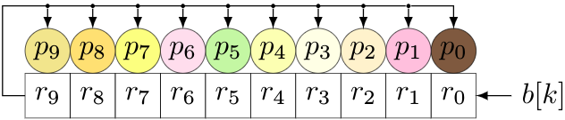
We would feed the bytes ( b[k] ) of the message in at the right; bytes ( r_0 ) through ( r_9 ) represent a remainder, and coefficients ( p_0 ) through ( p_9 ) represent the non-leading coefficients of the RS code’s generator polynomial. In this case, we would use a 10th-degree generator polynomial with a leading coefficient 1.
For each new byte, we do two things:
- Shift all cells left, shifting in one byte of the message
- Take the byte shifted out, and multiply it by the generator polynomial, then add (XOR) with the contents of the shift register.
We also have to remember to do this another ( n-k ) times (the length of the shift register) to cover the ( x^{n-k} ) factor. (Remember, we’re trying to calculate ( r(x) = x^{n-k}M(x) ).)
f256 = GF2QuotientRing(0x11d)

def rsencode_lfsr1(field, message, gtaps, remainder_only=False):
    """ encode a message in Reed-Solomon using LFSR
    field: symbol field
    message: string of bytes
    gtaps: generator polynomial coefficients, in ascending order
    remainder_only: whether to return the remainder only
    """
    glength = len(gtaps)
    remainder = np.zeros(glength, np.int)
    for char in message + ''*glength:
        remainder = np.roll(remainder, 1)
        out = remainder[0]
        remainder[0] = ord(char)
        for k, c in enumerate(gtaps):
            remainder[k] ^= field.mulraw(c, out)
    remainder = ''.join(chr(b) for b in reversed(remainder))
    return remainder if remainder_only else message+remainder

print rsencode_lfsr1(f256, msg, g[:-1], remainder_only=True).encode('hex')
print "calculated earlier:"
print remainder.encode('hex')
552ca3b464003a52c45011f46e0fea9b
calculated earlier:
552ca3b464003a52c45011f46e0fea9b
That worked, but we still have to handle multiplication in the symbol field, which is annoying and cumbersome for embedded processors. There are two table-driven methods that make this step easier, relegating the finite field stuff either to initialization steps only, or something that can be done at design time if you’re willing to generate a table in source code. (For example, using Python to generate the table coefficients in C.)
Also we have that call to np.roll(), which is too high-level for a language like C, so let’s look at things from this low-level, table-driven approach.
One table method is to take the generator polynomial and multiply it by each of the 256 possible coefficients, so that we get a table of 256 × ( n-k ) bytes.
def rsencode_lfsr2_table(field, gtaps):
    """
    Create a table for Reed-Solomon encoding using a field
    This time the taps are in *descending* order
    """
    return [[field.mulraw(b,c) for c in gtaps] for b in xrange(256)]

def rsencode_lfsr2(table, message, remainder_only=False):
    """ encode a message in Reed-Solomon using LFSR
    table: table[i][j] is the multiplication of
             generator coefficient of x^{n-k-1-j} by incoming byte i
    message: string of bytes
    remainder_only: whether to return the remainder only
    """
    glength = len(table[0])
    remainder = [0]*glength
    for char in message + ''*glength:
        out = remainder[0]
        table_row = table[out]
        for k in xrange(glength-1):
            remainder[k] = remainder[k+1] ^ table_row[k]
        remainder[glength-1] = ord(char) ^ table_row[glength-1]
    remainder = ''.join(chr(b) for b in remainder)
    return remainder if remainder_only else message+remainder

table = rsencode_lfsr2_table(f256, g[-2::-1])
print "table:"
for k, row in enumerate(table):
    print "%02x: %s" % (k, ' '.join('%02x' % c for c in row))
table:
00: 00 00 00 00 00 00 00 00 00 00 00 00 00 00 00 00
01: 3b 0d 68 bd 44 d1 1e 08 a3 41 29 e5 62 32 24 3b
02: 76 1a d0 67 88 bf 3c 10 5b 82 52 d7 c4 64 48 76
03: 4d 17 b8 da cc 6e 22 18 f8 c3 7b 32 a6 56 6c 4d
04: ec 34 bd ce 0d 63 78 20 b6 19 a4 b3 95 c8 90 ec
05: d7 39 d5 73 49 b2 66 28 15 58 8d 56 f7 fa b4 d7
06: 9a 2e 6d a9 85 dc 44 30 ed 9b f6 64 51 ac d8 9a
07: a1 23 05 14 c1 0d 5a 38 4e da df 81 33 9e fc a1
08: c5 68 67 81 1a c6 f0 40 71 32 55 7b 37 8d 3d c5
09: fe 65 0f 3c 5e 17 ee 48 d2 73 7c 9e 55 bf 19 fe
0a: b3 72 b7 e6 92 79 cc 50 2a b0 07 ac f3 e9 75 b3
0b: 88 7f df 5b d6 a8 d2 58 89 f1 2e 49 91 db 51 88
0c: 29 5c da 4f 17 a5 88 60 c7 2b f1 c8 a2 45 ad 29
0d: 12 51 b2 f2 53 74 96 68 64 6a d8 2d c0 77 89 12
0e: 5f 46 0a 28 9f 1a b4 70 9c a9 a3 1f 66 21 e5 5f
0f: 64 4b 62 95 db cb aa 78 3f e8 8a fa 04 13 c1 64
10: 97 d0 ce 1f 34 91 fd 80 e2 64 aa f6 6e 07 7a 97
11: ac dd a6 a2 70 40 e3 88 41 25 83 13 0c 35 5e ac
12: e1 ca 1e 78 bc 2e c1 90 b9 e6 f8 21 aa 63 32 e1
13: da c7 76 c5 f8 ff df 98 1a a7 d1 c4 c8 51 16 da
14: 7b e4 73 d1 39 f2 85 a0 54 7d 0e 45 fb cf ea 7b
15: 40 e9 1b 6c 7d 23 9b a8 f7 3c 27 a0 99 fd ce 40
16: 0d fe a3 b6 b1 4d b9 b0 0f ff 5c 92 3f ab a2 0d
17: 36 f3 cb 0b f5 9c a7 b8 ac be 75 77 5d 99 86 36
18: 52 b8 a9 9e 2e 57 0d c0 93 56 ff 8d 59 8a 47 52
19: 69 b5 c1 23 6a 86 13 c8 30 17 d6 68 3b b8 63 69
1a: 24 a2 79 f9 a6 e8 31 d0 c8 d4 ad 5a 9d ee 0f 24
1b: 1f af 11 44 e2 39 2f d8 6b 95 84 bf ff dc 2b 1f
1c: be 8c 14 50 23 34 75 e0 25 4f 5b 3e cc 42 d7 be
1d: 85 81 7c ed 67 e5 6b e8 86 0e 72 db ae 70 f3 85
1e: c8 96 c4 37 ab 8b 49 f0 7e cd 09 e9 08 26 9f c8
1f: f3 9b ac 8a ef 5a 57 f8 dd 8c 20 0c 6a 14 bb f3
20: 33 bd 81 3e 68 3f e7 1d d9 c8 49 f1 dc 0e f4 33
21: 08 b0 e9 83 2c ee f9 15 7a 89 60 14 be 3c d0 08
22: 45 a7 51 59 e0 80 db 0d 82 4a 1b 26 18 6a bc 45
23: 7e aa 39 e4 a4 51 c5 05 21 0b 32 c3 7a 58 98 7e
24: df 89 3c f0 65 5c 9f 3d 6f d1 ed 42 49 c6 64 df
25: e4 84 54 4d 21 8d 81 35 cc 90 c4 a7 2b f4 40 e4
26: a9 93 ec 97 ed e3 a3 2d 34 53 bf 95 8d a2 2c a9
27: 92 9e 84 2a a9 32 bd 25 97 12 96 70 ef 90 08 92
28: f6 d5 e6 bf 72 f9 17 5d a8 fa 1c 8a eb 83 c9 f6
29: cd d8 8e 02 36 28 09 55 0b bb 35 6f 89 b1 ed cd
2a: 80 cf 36 d8 fa 46 2b 4d f3 78 4e 5d 2f e7 81 80
2b: bb c2 5e 65 be 97 35 45 50 39 67 b8 4d d5 a5 bb
2c: 1a e1 5b 71 7f 9a 6f 7d 1e e3 b8 39 7e 4b 59 1a
2d: 21 ec 33 cc 3b 4b 71 75 bd a2 91 dc 1c 79 7d 21
2e: 6c fb 8b 16 f7 25 53 6d 45 61 ea ee ba 2f 11 6c
2f: 57 f6 e3 ab b3 f4 4d 65 e6 20 c3 0b d8 1d 35 57
30: a4 6d 4f 21 5c ae 1a 9d 3b ac e3 07 b2 09 8e a4
31: 9f 60 27 9c 18 7f 04 95 98 ed ca e2 d0 3b aa 9f
32: d2 77 9f 46 d4 11 26 8d 60 2e b1 d0 76 6d c6 d2
33: e9 7a f7 fb 90 c0 38 85 c3 6f 98 35 14 5f e2 e9
34: 48 59 f2 ef 51 cd 62 bd 8d b5 47 b4 27 c1 1e 48
35: 73 54 9a 52 15 1c 7c b5 2e f4 6e 51 45 f3 3a 73
36: 3e 43 22 88 d9 72 5e ad d6 37 15 63 e3 a5 56 3e
37: 05 4e 4a 35 9d a3 40 a5 75 76 3c 86 81 97 72 05
38: 61 05 28 a0 46 68 ea dd 4a 9e b6 7c 85 84 b3 61
39: 5a 08 40 1d 02 b9 f4 d5 e9 df 9f 99 e7 b6 97 5a
3a: 17 1f f8 c7 ce d7 d6 cd 11 1c e4 ab 41 e0 fb 17
3b: 2c 12 90 7a 8a 06 c8 c5 b2 5d cd 4e 23 d2 df 2c
3c: 8d 31 95 6e 4b 0b 92 fd fc 87 12 cf 10 4c 23 8d
3d: b6 3c fd d3 0f da 8c f5 5f c6 3b 2a 72 7e 07 b6
3e: fb 2b 45 09 c3 b4 ae ed a7 05 40 18 d4 28 6b fb
3f: c0 26 2d b4 87 65 b0 e5 04 44 69 fd b6 1a 4f c0
40: 66 67 1f 7c d0 7e d3 3a af 8d 92 ff a5 1c f5 66
41: 5d 6a 77 c1 94 af cd 32 0c cc bb 1a c7 2e d1 5d
42: 10 7d cf 1b 58 c1 ef 2a f4 0f c0 28 61 78 bd 10
43: 2b 70 a7 a6 1c 10 f1 22 57 4e e9 cd 03 4a 99 2b
44: 8a 53 a2 b2 dd 1d ab 1a 19 94 36 4c 30 d4 65 8a
45: b1 5e ca 0f 99 cc b5 12 ba d5 1f a9 52 e6 41 b1
46: fc 49 72 d5 55 a2 97 0a 42 16 64 9b f4 b0 2d fc
47: c7 44 1a 68 11 73 89 02 e1 57 4d 7e 96 82 09 c7
48: a3 0f 78 fd ca b8 23 7a de bf c7 84 92 91 c8 a3
49: 98 02 10 40 8e 69 3d 72 7d fe ee 61 f0 a3 ec 98
4a: d5 15 a8 9a 42 07 1f 6a 85 3d 95 53 56 f5 80 d5
4b: ee 18 c0 27 06 d6 01 62 26 7c bc b6 34 c7 a4 ee
4c: 4f 3b c5 33 c7 db 5b 5a 68 a6 63 37 07 59 58 4f
4d: 74 36 ad 8e 83 0a 45 52 cb e7 4a d2 65 6b 7c 74
4e: 39 21 15 54 4f 64 67 4a 33 24 31 e0 c3 3d 10 39
4f: 02 2c 7d e9 0b b5 79 42 90 65 18 05 a1 0f 34 02
50: f1 b7 d1 63 e4 ef 2e ba 4d e9 38 09 cb 1b 8f f1
51: ca ba b9 de a0 3e 30 b2 ee a8 11 ec a9 29 ab ca
52: 87 ad 01 04 6c 50 12 aa 16 6b 6a de 0f 7f c7 87
53: bc a0 69 b9 28 81 0c a2 b5 2a 43 3b 6d 4d e3 bc
54: 1d 83 6c ad e9 8c 56 9a fb f0 9c ba 5e d3 1f 1d
55: 26 8e 04 10 ad 5d 48 92 58 b1 b5 5f 3c e1 3b 26
56: 6b 99 bc ca 61 33 6a 8a a0 72 ce 6d 9a b7 57 6b
57: 50 94 d4 77 25 e2 74 82 03 33 e7 88 f8 85 73 50
58: 34 df b6 e2 fe 29 de fa 3c db 6d 72 fc 96 b2 34
59: 0f d2 de 5f ba f8 c0 f2 9f 9a 44 97 9e a4 96 0f
5a: 42 c5 66 85 76 96 e2 ea 67 59 3f a5 38 f2 fa 42
5b: 79 c8 0e 38 32 47 fc e2 c4 18 16 40 5a c0 de 79
5c: d8 eb 0b 2c f3 4a a6 da 8a c2 c9 c1 69 5e 22 d8
5d: e3 e6 63 91 b7 9b b8 d2 29 83 e0 24 0b 6c 06 e3
5e: ae f1 db 4b 7b f5 9a ca d1 40 9b 16 ad 3a 6a ae
5f: 95 fc b3 f6 3f 24 84 c2 72 01 b2 f3 cf 08 4e 95
60: 55 da 9e 42 b8 41 34 27 76 45 db 0e 79 12 01 55
61: 6e d7 f6 ff fc 90 2a 2f d5 04 f2 eb 1b 20 25 6e
62: 23 c0 4e 25 30 fe 08 37 2d c7 89 d9 bd 76 49 23
63: 18 cd 26 98 74 2f 16 3f 8e 86 a0 3c df 44 6d 18
64: b9 ee 23 8c b5 22 4c 07 c0 5c 7f bd ec da 91 b9
65: 82 e3 4b 31 f1 f3 52 0f 63 1d 56 58 8e e8 b5 82
66: cf f4 f3 eb 3d 9d 70 17 9b de 2d 6a 28 be d9 cf
67: f4 f9 9b 56 79 4c 6e 1f 38 9f 04 8f 4a 8c fd f4
68: 90 b2 f9 c3 a2 87 c4 67 07 77 8e 75 4e 9f 3c 90
69: ab bf 91 7e e6 56 da 6f a4 36 a7 90 2c ad 18 ab
6a: e6 a8 29 a4 2a 38 f8 77 5c f5 dc a2 8a fb 74 e6
6b: dd a5 41 19 6e e9 e6 7f ff b4 f5 47 e8 c9 50 dd
6c: 7c 86 44 0d af e4 bc 47 b1 6e 2a c6 db 57 ac 7c
6d: 47 8b 2c b0 eb 35 a2 4f 12 2f 03 23 b9 65 88 47
6e: 0a 9c 94 6a 27 5b 80 57 ea ec 78 11 1f 33 e4 0a
6f: 31 91 fc d7 63 8a 9e 5f 49 ad 51 f4 7d 01 c0 31
70: c2 0a 50 5d 8c d0 c9 a7 94 21 71 f8 17 15 7b c2
71: f9 07 38 e0 c8 01 d7 af 37 60 58 1d 75 27 5f f9
72: b4 10 80 3a 04 6f f5 b7 cf a3 23 2f d3 71 33 b4
73: 8f 1d e8 87 40 be eb bf 6c e2 0a ca b1 43 17 8f
74: 2e 3e ed 93 81 b3 b1 87 22 38 d5 4b 82 dd eb 2e
75: 15 33 85 2e c5 62 af 8f 81 79 fc ae e0 ef cf 15
76: 58 24 3d f4 09 0c 8d 97 79 ba 87 9c 46 b9 a3 58
77: 63 29 55 49 4d dd 93 9f da fb ae 79 24 8b 87 63
78: 07 62 37 dc 96 16 39 e7 e5 13 24 83 20 98 46 07
79: 3c 6f 5f 61 d2 c7 27 ef 46 52 0d 66 42 aa 62 3c
7a: 71 78 e7 bb 1e a9 05 f7 be 91 76 54 e4 fc 0e 71
7b: 4a 75 8f 06 5a 78 1b ff 1d d0 5f b1 86 ce 2a 4a
7c: eb 56 8a 12 9b 75 41 c7 53 0a 80 30 b5 50 d6 eb
7d: d0 5b e2 af df a4 5f cf f0 4b a9 d5 d7 62 f2 d0
7e: 9d 4c 5a 75 13 ca 7d d7 08 88 d2 e7 71 34 9e 9d
7f: a6 41 32 c8 57 1b 63 df ab c9 fb 02 13 06 ba a6
80: cc ce 3e f8 bd fc bb 74 43 07 39 e3 57 38 f7 cc
81: f7 c3 56 45 f9 2d a5 7c e0 46 10 06 35 0a d3 f7
82: ba d4 ee 9f 35 43 87 64 18 85 6b 34 93 5c bf ba
83: 81 d9 86 22 71 92 99 6c bb c4 42 d1 f1 6e 9b 81
84: 20 fa 83 36 b0 9f c3 54 f5 1e 9d 50 c2 f0 67 20
85: 1b f7 eb 8b f4 4e dd 5c 56 5f b4 b5 a0 c2 43 1b
86: 56 e0 53 51 38 20 ff 44 ae 9c cf 87 06 94 2f 56
87: 6d ed 3b ec 7c f1 e1 4c 0d dd e6 62 64 a6 0b 6d
88: 09 a6 59 79 a7 3a 4b 34 32 35 6c 98 60 b5 ca 09
89: 32 ab 31 c4 e3 eb 55 3c 91 74 45 7d 02 87 ee 32
8a: 7f bc 89 1e 2f 85 77 24 69 b7 3e 4f a4 d1 82 7f
8b: 44 b1 e1 a3 6b 54 69 2c ca f6 17 aa c6 e3 a6 44
8c: e5 92 e4 b7 aa 59 33 14 84 2c c8 2b f5 7d 5a e5
8d: de 9f 8c 0a ee 88 2d 1c 27 6d e1 ce 97 4f 7e de
8e: 93 88 34 d0 22 e6 0f 04 df ae 9a fc 31 19 12 93
8f: a8 85 5c 6d 66 37 11 0c 7c ef b3 19 53 2b 36 a8
90: 5b 1e f0 e7 89 6d 46 f4 a1 63 93 15 39 3f 8d 5b
91: 60 13 98 5a cd bc 58 fc 02 22 ba f0 5b 0d a9 60
92: 2d 04 20 80 01 d2 7a e4 fa e1 c1 c2 fd 5b c5 2d
93: 16 09 48 3d 45 03 64 ec 59 a0 e8 27 9f 69 e1 16
94: b7 2a 4d 29 84 0e 3e d4 17 7a 37 a6 ac f7 1d b7
95: 8c 27 25 94 c0 df 20 dc b4 3b 1e 43 ce c5 39 8c
96: c1 30 9d 4e 0c b1 02 c4 4c f8 65 71 68 93 55 c1
97: fa 3d f5 f3 48 60 1c cc ef b9 4c 94 0a a1 71 fa
98: 9e 76 97 66 93 ab b6 b4 d0 51 c6 6e 0e b2 b0 9e
99: a5 7b ff db d7 7a a8 bc 73 10 ef 8b 6c 80 94 a5
9a: e8 6c 47 01 1b 14 8a a4 8b d3 94 b9 ca d6 f8 e8
9b: d3 61 2f bc 5f c5 94 ac 28 92 bd 5c a8 e4 dc d3
9c: 72 42 2a a8 9e c8 ce 94 66 48 62 dd 9b 7a 20 72
9d: 49 4f 42 15 da 19 d0 9c c5 09 4b 38 f9 48 04 49
9e: 04 58 fa cf 16 77 f2 84 3d ca 30 0a 5f 1e 68 04
9f: 3f 55 92 72 52 a6 ec 8c 9e 8b 19 ef 3d 2c 4c 3f
a0: ff 73 bf c6 d5 c3 5c 69 9a cf 70 12 8b 36 03 ff
a1: c4 7e d7 7b 91 12 42 61 39 8e 59 f7 e9 04 27 c4
a2: 89 69 6f a1 5d 7c 60 79 c1 4d 22 c5 4f 52 4b 89
a3: b2 64 07 1c 19 ad 7e 71 62 0c 0b 20 2d 60 6f b2
a4: 13 47 02 08 d8 a0 24 49 2c d6 d4 a1 1e fe 93 13
a5: 28 4a 6a b5 9c 71 3a 41 8f 97 fd 44 7c cc b7 28
a6: 65 5d d2 6f 50 1f 18 59 77 54 86 76 da 9a db 65
a7: 5e 50 ba d2 14 ce 06 51 d4 15 af 93 b8 a8 ff 5e
a8: 3a 1b d8 47 cf 05 ac 29 eb fd 25 69 bc bb 3e 3a
a9: 01 16 b0 fa 8b d4 b2 21 48 bc 0c 8c de 89 1a 01
aa: 4c 01 08 20 47 ba 90 39 b0 7f 77 be 78 df 76 4c
ab: 77 0c 60 9d 03 6b 8e 31 13 3e 5e 5b 1a ed 52 77
ac: d6 2f 65 89 c2 66 d4 09 5d e4 81 da 29 73 ae d6
ad: ed 22 0d 34 86 b7 ca 01 fe a5 a8 3f 4b 41 8a ed
ae: a0 35 b5 ee 4a d9 e8 19 06 66 d3 0d ed 17 e6 a0
af: 9b 38 dd 53 0e 08 f6 11 a5 27 fa e8 8f 25 c2 9b
b0: 68 a3 71 d9 e1 52 a1 e9 78 ab da e4 e5 31 79 68
b1: 53 ae 19 64 a5 83 bf e1 db ea f3 01 87 03 5d 53
b2: 1e b9 a1 be 69 ed 9d f9 23 29 88 33 21 55 31 1e
b3: 25 b4 c9 03 2d 3c 83 f1 80 68 a1 d6 43 67 15 25
b4: 84 97 cc 17 ec 31 d9 c9 ce b2 7e 57 70 f9 e9 84
b5: bf 9a a4 aa a8 e0 c7 c1 6d f3 57 b2 12 cb cd bf
b6: f2 8d 1c 70 64 8e e5 d9 95 30 2c 80 b4 9d a1 f2
b7: c9 80 74 cd 20 5f fb d1 36 71 05 65 d6 af 85 c9
b8: ad cb 16 58 fb 94 51 a9 09 99 8f 9f d2 bc 44 ad
b9: 96 c6 7e e5 bf 45 4f a1 aa d8 a6 7a b0 8e 60 96
ba: db d1 c6 3f 73 2b 6d b9 52 1b dd 48 16 d8 0c db
bb: e0 dc ae 82 37 fa 73 b1 f1 5a f4 ad 74 ea 28 e0
bc: 41 ff ab 96 f6 f7 29 89 bf 80 2b 2c 47 74 d4 41
bd: 7a f2 c3 2b b2 26 37 81 1c c1 02 c9 25 46 f0 7a
be: 37 e5 7b f1 7e 48 15 99 e4 02 79 fb 83 10 9c 37
bf: 0c e8 13 4c 3a 99 0b 91 47 43 50 1e e1 22 b8 0c
c0: aa a9 21 84 6d 82 68 4e ec 8a ab 1c f2 24 02 aa
c1: 91 a4 49 39 29 53 76 46 4f cb 82 f9 90 16 26 91
c2: dc b3 f1 e3 e5 3d 54 5e b7 08 f9 cb 36 40 4a dc
c3: e7 be 99 5e a1 ec 4a 56 14 49 d0 2e 54 72 6e e7
c4: 46 9d 9c 4a 60 e1 10 6e 5a 93 0f af 67 ec 92 46
c5: 7d 90 f4 f7 24 30 0e 66 f9 d2 26 4a 05 de b6 7d
c6: 30 87 4c 2d e8 5e 2c 7e 01 11 5d 78 a3 88 da 30
c7: 0b 8a 24 90 ac 8f 32 76 a2 50 74 9d c1 ba fe 0b
c8: 6f c1 46 05 77 44 98 0e 9d b8 fe 67 c5 a9 3f 6f
c9: 54 cc 2e b8 33 95 86 06 3e f9 d7 82 a7 9b 1b 54
ca: 19 db 96 62 ff fb a4 1e c6 3a ac b0 01 cd 77 19
cb: 22 d6 fe df bb 2a ba 16 65 7b 85 55 63 ff 53 22
cc: 83 f5 fb cb 7a 27 e0 2e 2b a1 5a d4 50 61 af 83
cd: b8 f8 93 76 3e f6 fe 26 88 e0 73 31 32 53 8b b8
ce: f5 ef 2b ac f2 98 dc 3e 70 23 08 03 94 05 e7 f5
cf: ce e2 43 11 b6 49 c2 36 d3 62 21 e6 f6 37 c3 ce
d0: 3d 79 ef 9b 59 13 95 ce 0e ee 01 ea 9c 23 78 3d
d1: 06 74 87 26 1d c2 8b c6 ad af 28 0f fe 11 5c 06
d2: 4b 63 3f fc d1 ac a9 de 55 6c 53 3d 58 47 30 4b
d3: 70 6e 57 41 95 7d b7 d6 f6 2d 7a d8 3a 75 14 70
d4: d1 4d 52 55 54 70 ed ee b8 f7 a5 59 09 eb e8 d1
d5: ea 40 3a e8 10 a1 f3 e6 1b b6 8c bc 6b d9 cc ea
d6: a7 57 82 32 dc cf d1 fe e3 75 f7 8e cd 8f a0 a7
d7: 9c 5a ea 8f 98 1e cf f6 40 34 de 6b af bd 84 9c
d8: f8 11 88 1a 43 d5 65 8e 7f dc 54 91 ab ae 45 f8
d9: c3 1c e0 a7 07 04 7b 86 dc 9d 7d 74 c9 9c 61 c3
da: 8e 0b 58 7d cb 6a 59 9e 24 5e 06 46 6f ca 0d 8e
db: b5 06 30 c0 8f bb 47 96 87 1f 2f a3 0d f8 29 b5
dc: 14 25 35 d4 4e b6 1d ae c9 c5 f0 22 3e 66 d5 14
dd: 2f 28 5d 69 0a 67 03 a6 6a 84 d9 c7 5c 54 f1 2f
de: 62 3f e5 b3 c6 09 21 be 92 47 a2 f5 fa 02 9d 62
df: 59 32 8d 0e 82 d8 3f b6 31 06 8b 10 98 30 b9 59
e0: 99 14 a0 ba 05 bd 8f 53 35 42 e2 ed 2e 2a f6 99
e1: a2 19 c8 07 41 6c 91 5b 96 03 cb 08 4c 18 d2 a2
e2: ef 0e 70 dd 8d 02 b3 43 6e c0 b0 3a ea 4e be ef
e3: d4 03 18 60 c9 d3 ad 4b cd 81 99 df 88 7c 9a d4
e4: 75 20 1d 74 08 de f7 73 83 5b 46 5e bb e2 66 75
e5: 4e 2d 75 c9 4c 0f e9 7b 20 1a 6f bb d9 d0 42 4e
e6: 03 3a cd 13 80 61 cb 63 d8 d9 14 89 7f 86 2e 03
e7: 38 37 a5 ae c4 b0 d5 6b 7b 98 3d 6c 1d b4 0a 38
e8: 5c 7c c7 3b 1f 7b 7f 13 44 70 b7 96 19 a7 cb 5c
e9: 67 71 af 86 5b aa 61 1b e7 31 9e 73 7b 95 ef 67
ea: 2a 66 17 5c 97 c4 43 03 1f f2 e5 41 dd c3 83 2a
eb: 11 6b 7f e1 d3 15 5d 0b bc b3 cc a4 bf f1 a7 11
ec: b0 48 7a f5 12 18 07 33 f2 69 13 25 8c 6f 5b b0
ed: 8b 45 12 48 56 c9 19 3b 51 28 3a c0 ee 5d 7f 8b
ee: c6 52 aa 92 9a a7 3b 23 a9 eb 41 f2 48 0b 13 c6
ef: fd 5f c2 2f de 76 25 2b 0a aa 68 17 2a 39 37 fd
f0: 0e c4 6e a5 31 2c 72 d3 d7 26 48 1b 40 2d 8c 0e
f1: 35 c9 06 18 75 fd 6c db 74 67 61 fe 22 1f a8 35
f2: 78 de be c2 b9 93 4e c3 8c a4 1a cc 84 49 c4 78
f3: 43 d3 d6 7f fd 42 50 cb 2f e5 33 29 e6 7b e0 43
f4: e2 f0 d3 6b 3c 4f 0a f3 61 3f ec a8 d5 e5 1c e2
f5: d9 fd bb d6 78 9e 14 fb c2 7e c5 4d b7 d7 38 d9
f6: 94 ea 03 0c b4 f0 36 e3 3a bd be 7f 11 81 54 94
f7: af e7 6b b1 f0 21 28 eb 99 fc 97 9a 73 b3 70 af
f8: cb ac 09 24 2b ea 82 93 a6 14 1d 60 77 a0 b1 cb
f9: f0 a1 61 99 6f 3b 9c 9b 05 55 34 85 15 92 95 f0
fa: bd b6 d9 43 a3 55 be 83 fd 96 4f b7 b3 c4 f9 bd
fb: 86 bb b1 fe e7 84 a0 8b 5e d7 66 52 d1 f6 dd 86
fc: 27 98 b4 ea 26 89 fa b3 10 0d b9 d3 e2 68 21 27
fd: 1c 95 dc 57 62 58 e4 bb b3 4c 90 36 80 5a 05 1c
fe: 51 82 64 8d ae 36 c6 a3 4b 8f eb 04 26 0c 69 51
ff: 6a 8f 0c 30 ea e7 d8 ab e8 ce c2 e1 44 3e 4d 6a
print rsencode_lfsr2(table, msg, remainder_only=True).encode('hex')
print "calculated earlier:"
print remainder.encode('hex')
552ca3b464003a52c45011f46e0fea9b
calculated earlier:
552ca3b464003a52c45011f46e0fea9b
Alternatively, if none of the generating polynomial’s coefficients are zero, we can just represent these coefficients as powers of a generating element of a field, and then store log and antilog tables of ( x^n ) in the symbol field. These are each a smaller table of length 256 (with one dummy entry) and they remove all dependencies on doing arithmetic in the symbol field.
def rsencode_lfsr3_table(field_polynomial):
    """
    Create log and antilog tables for Reed-Solomon encoding using a field
    This just uses powers of x^n.
    """
    log = [0] * 256
    antilog = [0] * 256
    c = 1
    for k in xrange(255):
        antilog[k] = c
        log[c] = k
        c <<= 1
        cxor = c ^ field_polynomial
        if cxor < c:
            c = cxor
    return log, antilog

def rsencode_lfsr3(log, antilog, gpowers, message, remainder_only=False):
    """ encode a message in Reed-Solomon using LFSR
    log, antilog: tables for log and antilog: log[x^i] = i, antilog[i] = x^i
    gpowers: generator polynomial coefficients x^i, represented as i, in descending order
    message: string of bytes
    remainder_only: whether to return the remainder only
    """
    glength = len(gpowers)
    remainder = [0]*glength
    for char in message + ''*glength:
        out = remainder[0]
        if out == 0:
            # No multiplication. Just shift.
            for k in xrange(glength-1):
                remainder[k] = remainder[k+1]
            remainder[glength-1] = ord(char)
        else:
            outp = log[out]
            for k in xrange(glength-1):
                j = gpowers[k] + outp
                if j >= 255:
                    j -= 255
                remainder[k] = remainder[k+1] ^ antilog[j]
            j = gpowers[glength-1] + outp
            if j >= 255:
                j -= 255
            remainder[glength-1] = ord(char) ^ antilog[j]
    remainder = ''.join(chr(b) for b in remainder)
    return remainder if remainder_only else message+remainder

log, antilog = rsencode_lfsr3_table(f256.coeffs)
for (name, table) in [('log',log),('antilog',antilog)]:
    print "%s:" % name
    for k in xrange(0,256,16):
        print "%03d-%03d: %s" % (k,k+15,
                ' '.join('%02x' % c for c in table[k:k+16]))
log:
000-015: 00 00 01 19 02 32 1a c6 03 df 33 ee 1b 68 c7 4b
016-031: 04 64 e0 0e 34 8d ef 81 1c c1 69 f8 c8 08 4c 71
032-047: 05 8a 65 2f e1 24 0f 21 35 93 8e da f0 12 82 45
048-063: 1d b5 c2 7d 6a 27 f9 b9 c9 9a 09 78 4d e4 72 a6
064-079: 06 bf 8b 62 66 dd 30 fd e2 98 25 b3 10 91 22 88
080-095: 36 d0 94 ce 8f 96 db bd f1 d2 13 5c 83 38 46 40
096-111: 1e 42 b6 a3 c3 48 7e 6e 6b 3a 28 54 fa 85 ba 3d
112-127: ca 5e 9b 9f 0a 15 79 2b 4e d4 e5 ac 73 f3 a7 57
128-143: 07 70 c0 f7 8c 80 63 0d 67 4a de ed 31 c5 fe 18
144-159: e3 a5 99 77 26 b8 b4 7c 11 44 92 d9 23 20 89 2e
160-175: 37 3f d1 5b 95 bc cf cd 90 87 97 b2 dc fc be 61
176-191: f2 56 d3 ab 14 2a 5d 9e 84 3c 39 53 47 6d 41 a2
192-207: 1f 2d 43 d8 b7 7b a4 76 c4 17 49 ec 7f 0c 6f f6
208-223: 6c a1 3b 52 29 9d 55 aa fb 60 86 b1 bb cc 3e 5a
224-239: cb 59 5f b0 9c a9 a0 51 0b f5 16 eb 7a 75 2c d7
240-255: 4f ae d5 e9 e6 e7 ad e8 74 d6 f4 ea a8 50 58 af
antilog:
000-015: 01 02 04 08 10 20 40 80 1d 3a 74 e8 cd 87 13 26
016-031: 4c 98 2d 5a b4 75 ea c9 8f 03 06 0c 18 30 60 c0
032-047: 9d 27 4e 9c 25 4a 94 35 6a d4 b5 77 ee c1 9f 23
048-063: 46 8c 05 0a 14 28 50 a0 5d ba 69 d2 b9 6f de a1
064-079: 5f be 61 c2 99 2f 5e bc 65 ca 89 0f 1e 3c 78 f0
080-095: fd e7 d3 bb 6b d6 b1 7f fe e1 df a3 5b b6 71 e2
096-111: d9 af 43 86 11 22 44 88 0d 1a 34 68 d0 bd 67 ce
112-127: 81 1f 3e 7c f8 ed c7 93 3b 76 ec c5 97 33 66 cc
128-143: 85 17 2e 5c b8 6d da a9 4f 9e 21 42 84 15 2a 54
144-159: a8 4d 9a 29 52 a4 55 aa 49 92 39 72 e4 d5 b7 73
160-175: e6 d1 bf 63 c6 91 3f 7e fc e5 d7 b3 7b f6 f1 ff
176-191: e3 db ab 4b 96 31 62 c4 95 37 6e dc a5 57 ae 41
192-207: 82 19 32 64 c8 8d 07 0e 1c 38 70 e0 dd a7 53 a6
208-223: 51 a2 59 b2 79 f2 f9 ef c3 9b 2b 56 ac 45 8a 09
224-239: 12 24 48 90 3d 7a f4 f5 f7 f3 fb eb cb 8b 0b 16
240-255: 2c 58 b0 7d fa e9 cf 83 1b 36 6c d8 ad 47 8e 00
gpowers = [log[c] for c in g[-2::-1]]
print "generator polynomial coefficient indices: ", gpowers
print "remainder:"
print rsencode_lfsr3(log, antilog, gpowers, msg, remainder_only=True).encode('hex')
print "calculated earlier:"
print remainder.encode('hex')
generator polynomial coefficient indices:  [120, 104, 107, 109, 102, 161, 76, 3, 91, 191, 147, 169, 182, 194, 225, 120]
remainder:
552ca3b464003a52c45011f46e0fea9b
calculated earlier:
552ca3b464003a52c45011f46e0fea9b
There. It’s very simple; the hardest thing here is making sure you get the coefficients in the right order. You wouldn’t want to get those the wrong way around.
C Implementation
I tested a C implementation using XC16 and the MPLAB X debugger:
""" C code for reed-solomon.c:
/*
 *
 * Copyright 2018 Jason M. Sachs
 *
 * Licensed under the Apache License, Version 2.0 (the "License");
 * you may not use this file except in compliance with the License.
 * You may obtain a copy of the License at
 *
 *   http://www.apache.org/licenses/LICENSE-2.0
 *
 * Unless required by applicable law or agreed to in writing, software
 * distributed under the License is distributed on an "AS IS" BASIS,
 * WITHOUT WARRANTIES OR CONDITIONS OF ANY KIND, either express or implied.
 * See the License for the specific language governing permissions and
 * limitations under the License.
 */

#include <stdint.h>
#include <stddef.h>
#include <string.h>

/**
 * Reed-Solomon log-table-based implementation
 */
typedef struct {
    uint8_t log[256];
    uint8_t antilog[256];
    uint8_t symbol_polynomial;
    const uint8_t *gpowers;
    uint8_t generator_degree;
} rslogtable_t;


/**
 * Initialize log table
 *
 * @param ptables - points to log tables
 * @param symbol_polynomial: lower 8 bits of symbol polynomial
 *         (for example, 0x1d for 0x11d = x^8 + x^4 + x^3 + x^2 + 1
 * @param gpowers - points to generator polynomial coefficients,
 *         except for the leading monomial,
 *         in descending order, expressed as powers of x in the symbol field.
 *         This requires all generator polynomial coefficients to be nonzero.
 * @param generator_degree - degree of the generator polynomial,
 *         which is also the length of the gpowers array.
 */
void rslogtable_init(
    rslogtable_t *ptables,
    uint8_t symbol_polynomial,
    const uint8_t *gpowers,
    uint8_t generator_degree
)
{
    ptables->symbol_polynomial = symbol_polynomial;
    ptables->gpowers = gpowers;
    ptables->generator_degree = generator_degree;

    int k;
    uint8_t c = 1;
    for (k = 0; k < 255; ++k)
    {
        ptables->antilog[k] = c;
        ptables->log[c] = k;
        if (c >> 7)
        {
            c <<= 1;
            c ^= symbol_polynomial;
        }
        else
        {
            c <<= 1;
        }
    }
    ptables->log[0] = 0;
    ptables->antilog[255] = 0;
}

/**
 * Encode a message
 *
 * @param ptables - pointer to table-based lookup info
 * @param pmessage - message to be encoded
 * @param message_length - length of the message
 * @param premainder - buffer which will be filled in with the remainder.
 *     This must have a size equal to ptables->generator_degree
 */
void rslogtable_encode(
    const rslogtable_t *ptables,
    const uint8_t *pmessage,
    size_t message_length,
    uint8_t *premainder
)
{
    int i, j, k, n;
    int highbyte;
    const int t2 = ptables->generator_degree;
    const int lastindex = t2-1;

    // Zero out the remainder
    for (i = 0; i < t2; ++i)
    {
        premainder[i] = 0;
    }

    n = message_length + t2;
    for (i = 0; i < n; ++i)
    {
        uint8_t c = (i < message_length) ? pmessage[i] : 0;
        highbyte = premainder[0];
        if (highbyte == 0)
        {
            // No multiplication, just a simple shift
            for (k = 0; k < lastindex; ++k)
            {
                premainder[k] = premainder[k+1];
            }
            premainder[lastindex] = c;
        }
        else
        {
            uint8_t log_highbyte = ptables->log[highbyte];
            for (k = 0; k < lastindex; ++k)
            {
                j = ptables->gpowers[k] + (int)log_highbyte;
                if (j >= 255)
                    j -= 255;
                premainder[k] = premainder[k+1] ^ ptables->antilog[j];
            }
            j = ptables->gpowers[lastindex] + (int)log_highbyte;
            if (j >= 255)
                j -= 255;
            premainder[lastindex] = c ^ ptables->antilog[j];
        }
    }
}

uint8_t rsremainder[16];
void rslogtable_test(void)
{
    const uint8_t gpowers[] = {
        120, 104, 107, 109,
        102, 161, 76, 3,
        91, 191, 147, 169,
        182, 194, 225, 120
    };
    rslogtable_t rsinfo;
    rslogtable_init(&rsinfo, 0x1d, gpowers, 16);

    const char message[] = "Ernie, you have a banana in your ear!";
    rslogtable_encode(&rsinfo, (const uint8_t *)message, strlen(message), rsremainder);
    __builtin_nop();
}
""";
It worked as expected:
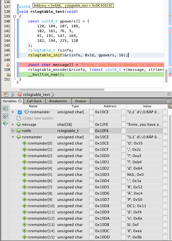
Again, this is only the encoder, but remember the asymmetry here:
- encoder = cheap resource-limited processor
- decoder = desktop PC CPU
And we can still do error correction!
Is It Worth It?
Is encoding worth the effort?
Wait. We got all the way through Part XV and well into this article, you say, and he’s asking is it worth it?!
Yes, that’s the question. We got a benefit, namely the ability to detect and sometimes even correct errors, but it has a cost. We have to send extra information, and that uses up part of the available communications bandwidth. And we had to add some complexity. Is it a net gain?
There are at least two ways of looking at this cost-benefit tradeoff, and it depends on what the constraints are.
The first way of analyzing cost-benefits is to consider a situation where we’re given a transmitter/receiver pair, and all we have control over is the digital part of the system that handles the bits that are sent. Error correcting codes like Reed-Solomon give us the ability to lower the error rate substantially — and we’ll calculate this in just a minute — with only a slight decrease in transmission rate. A ( (255, 239) ) Reed-Solomon code lets us correct up to 8 errors in each block of 255 bytes, with 93.7% of the transmission capacity of the uncoded channel. The encoding complexity cost is minimal, and the decoding cost is small enough to merit use of Reed-Solomon decoders in higher-end embedded systems or in desktop computers.
The second way of analyzing cost-benefits is to consider a situation where we have control over the transmitter energy, as well as the digital encoding/decoding mechanisms. We can lower the error rate by using an error-correcting code, or we can increase the transmitter energy to improve the signal-to-noise ratio. The Shannon-Hartley theorem, which says channel capacity ( C leq B log_2 (1+frac{S}{N}) ), can help us quantitatively compare those possibilities. The standard metric is ( E_b/N_0 ) in decibels, so let’s try to frame things in terms of it. First we have to understand what it is.
One common assumption in communications is an additive Gaussian white noise (AWGN) channel, which has some amount of noise ( N_0 ) per unit bandwidth. This is why oscilloscopes let you limit the bandwidth; if you don’t need it, it reduces the noise level. In any case, if we have an integrate-and-dump receiver, where we integrate our received signal, and every ( T ) seconds we sample the integrator value, divide by ( T ) to compute an average value over the interval, and reset the integrator, then the received noise can be modeled as a Gaussian random variable with zero mean and variance of ( sigma_N^2 = frac{N_0}{2T} ). (This can be computed from ( sigma_N^2 = frac{N_0}{2}int_{-infty}^{infty}left|h(t)right|^2, dt ) with ( h(t) ) of the integrate-and-dump filter being a unit rectangular pulse of duration ( T ) and height ( 1/T ).)
The signal waveform has some energy ( E_b ) per bit. Consider a raw binary pulse signal ( x(t) = pm A ) for a duration of ( T ) seconds for each bit, with ( +A ) representing a binary 1 and ( -A ) representing a binary 0. If we compute ( E_b = int_{-infty}^{infty}left|x(t)right|^2, dt ) we get ( E_b = A^2T ). The integrate-and-dump receiver outputs a 1 if its output sample is positive, and 0 if its output sample is negative. We get a bit flip if the received noise is less than ( -A ) for a transmitted 1 bit, or greater than ( A ) for a transmitted 0 bit. This probability is just the Q-function evaluated at ( Q(A/sigma_n) = Q(sqrt{A^2/sigma_n{}^2}) = Q(sqrt{(E_b/T)/(N_0/2T)}) = Q(sqrt{2E_b/N_0}). )
In other words, if we know how bits are represented as signals, we can determine the probability of a bit error just by knowing what ( E_b/N_0 ) is.
Let’s graph it!
Bit Error Rate Calculations Are the Bane of My Existence
Just one quick aside: this section showing bit error rate graphs was a beastly thing to manage. Don’t worry about the Python code, or how the calculations work, unless you want to enter this quagmire. Otherwise, just look at the pretty pictures, and my descriptions of how to interpret them.
As I was saying, let’s graph it!
import numpy as np
import pandas as pd
import matplotlib.pyplot as plt
%matplotlib inline
import scipy.stats

def Q(x):
    return scipy.stats.norm.cdf(-x)

def Qinv(x):
    return -scipy.stats.norm.ppf(x)

ebno_db = np.arange(-6,12,0.01)
ebno = 10**(ebno_db/10)
# Decibels are often confusing.
# dB = 10 log10 x  if x is measured in energy
# dB = 20 log10 x  if x is measured in amplitude.

plt.semilogy(ebno_db, Q(np.sqrt(2*ebno)))
plt.ylabel('Bit error rate',fontsize=12)
plt.xlabel('$E_b/N_0$ (dB)',fontsize=12)
plt.grid('on')
plt.title('Bit error rate for raw binary pulses in AWGN channeln'
          +'with integrate-and-dump receiver');
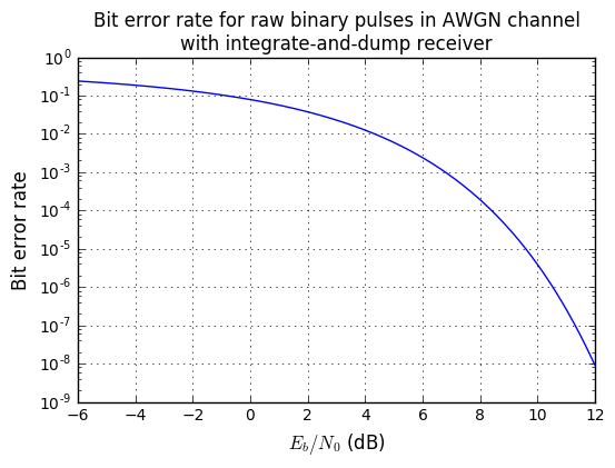
If we have a nice healthy noise margin of 12dB for ( E_b/N_0 ), then the bit error rate is ( 9.0times 10^{-9} ), or one error in 110 million. Again, this is just raw binary pulses using an integrate-and-dump receiver. More complex signal shaping techniques like quadrature amplitude modulation can make better use of available spectrum. But that’s an article for someone else to write.
With an ( E_b/N_0 ) ratio of 1 (that’s 0dB), probability of a bit error is around 0.079, or about one in 12. Lousy. You want a lower error rate? Put more energy into the signal, or make sure there’s less energy in noise.
Okay, now suppose we use a Hamming (7,4) code. Let’s say, for example, that the raw bit error rate is 0.01, which occurs at about ( E_b/N_0 approx 4.3 )dB. With the Hamming (7,4) code, we can correct one error, so there are a few cases to consider for an upper bound that is conservative and assumes some worst-case conditions:
- There were no received bit errors. Probability of this is ( (1-0.01)^7 approx 0.932065. ) The receiver will output 4 correct output bits, and there are no errors after decoding
- There was one received bit error, in one of the seven codeword bits. Probability of this is ( 7cdot 0.01cdot(1-0.01)^6 approx 0.065904. ) The receiver will output 4 correct output bits, and there are no errors after decoding.
- There are two or more received bit errors. Probability of this is ( approx 0.002031 ). We don’t know how many correct output bits the receiver will produce; a true analysis is complicated. Let’s just assume, as a worst-case estimate, we’ll receive no correct output bits, so there are 4 errors after decoding.
In this case the expected number of errors (worst-case) in the output bits is 4 × 0.002031, or 0.002031 per output bit.
We went from a bit error rate of 0.01 down to about 0.002031, which is good, right? The only drawback is that to send data 4 bits we had to transmit 7 bits, so the transmitted energy per bit is a factor of 7/4 higher.
We can find the expected number of errors more precisely if we look at the received error count for each combination of the 128 possible error patterns, and compute the “weighted count” W as the sum of the received error counts, weighted by the number of patterns that cause that combination of raw and received error count:
# stuff from Part XV
def hamming74_decode(codeword, return_syndrome=False):
    qr = GF2QuotientRing(0b1011)
    beta = 0b111
    syndrome = 0
    bitpos = 1 << 7
    # clock in the codeword, then three zero bits
    for k in xrange(10):
        syndrome = qr.lshiftraw1(syndrome)
        if codeword & bitpos:
            syndrome ^= 1
        bitpos >>= 1
    data = codeword & 0xf
    if syndrome == 0:
        error_pos=None
    else:
        # there are easier ways of computing a correction
        # to the data bits (I'm just not familiar with them)
        error_pos=qr.log(qr.mulraw(syndrome,beta))
        if error_pos < 4:
            data ^= (1<<error_pos)
    if return_syndrome:
        return data, syndrome, error_pos
    else:
        return data

# Find syndromes and error positions for basis vectors (all 1)
# and construct syndromes for all 128 possible values using linearity

syndrome_to_correction_mask = np.zeros(8, dtype=int)
patterns = np.arange(128)
syndromes = np.zeros(128, dtype=int)
bit_counts = np.zeros(128, dtype=int)
for i in xrange(7):
    error_pattern = 1<<i
    data, syndrome, error_pos = hamming74_decode(error_pattern, return_syndrome=True)
    assert error_pos == i
    syndrome_to_correction_mask[syndrome] = error_pattern
    bitmatch = (patterns & error_pattern) != 0
    syndromes[bitmatch] ^= syndrome
    bit_counts[bitmatch] += 1

correction_mask = syndrome_to_correction_mask[syndromes[patterns]]
corrected_patterns = patterns ^ correction_mask
received_error_count = bit_counts[corrected_patterns & 0xF]
# determine the number of errors in the corrected data bits

H74_table = pd.DataFrame(dict(pattern=patterns,
                       raw_error_count=bit_counts,
                       correction_mask=correction_mask,
                       corrected_pattern=corrected_patterns,
                       received_error_count=received_error_count
                       ),
                  columns=['pattern',
                        'correction_mask','corrected_pattern',
                        'raw_error_count','received_error_count'])
H74_stats = (H74_table
          .groupby(['raw_error_count','received_error_count'])
          .agg({'pattern': 'count'})
          .rename(columns={'pattern':'count'}))

H74_stats
| count | ||
|---|---|---|
| raw_error_count | received_error_count | |
| 0 | 0 | 1 |
| 1 | 0 | 7 |
| 2 | 1 | 9 |
| 2 | 9 | |
| 3 | 3 | |
| 3 | 1 | 7 |
| 2 | 15 | |
| 3 | 13 | |
| 4 | 1 | 13 |
| 2 | 15 | |
| 3 | 7 | |
| 5 | 1 | 3 |
| 2 | 9 | |
| 3 | 9 | |
| 6 | 4 | 7 |
| 7 | 4 | 1 |
H74a = H74_stats.reset_index()
H74b_data = [
    ('raw_error_count',H74a['raw_error_count']),
    ('weighted_count',)
]
H74b = ((H74a['received_error_count']*H74a['count'])
        .groupby(H74a['raw_error_count'])
        .agg({'weighted_count':'sum'}))
H74b
| weighted_count | |
|---|---|
| raw_error_count | |
| 0 | 0 |
| 1 | 0 |
| 2 | 36 |
| 3 | 76 |
| 4 | 64 |
| 5 | 48 |
| 6 | 28 |
| 7 | 4 |
This then lets us calculate the net error rate as ( (W_0(1-p)^7 + W_1 p(1-p)^6 + W_2 p^2(1-p)^5 + ldots + W_6p^6(1-p) + W_7p^7) / 4 ):
W = H74b['weighted_count']
p = 0.01
r = sum(W[i]*(1-p)**(7-i)*p**i for i in xrange(8))/4
r
Even better!
Now let’s look at that bit error rate graph again, this time with both the curve for uncoded data, and with another curve representing the use of a Hamming (7,4) code.
# Helper functions for analyzing small Hamming codes (7,4) and (15,11)
# and Reed-Solomon(255,k) codes

import scipy.misc
import scipy.stats

class HammingAnalyzer(object):
    def __init__(self, poly):
        self.qr = GF2QuotientRing(poly)
        self.nparity = self.qr.degree
        self.n = (1 << self.nparity) - 1
        self.k = self.n - self.nparity
        self.beta = self._calculate_beta()
        assert self.decode(1<<self.k) == 0
        self.W = None
    def _calculate_beta(self):
        syndrome_msb = self.calculate_syndrome(1<<self.k)
        msb_pattern = self.qr.lshiftraw(1, self.k)
        beta = self.qr.divraw(msb_pattern, syndrome_msb)
        # Beta is calculated such that beta * syndrome(M) = M
        # for M = a codeword of all zeros with bit k = 1
        # (all data bits are zero)
        return beta
    def calculate_syndrome(self, codeword):
        syndrome = 0
        bitpos = 1 << self.n
        # clock in the codeword, then enough bits to cover the parity bits
        for _ in xrange(self.n + self.nparity):
            syndrome = self.qr.lshiftraw1(syndrome)
            if codeword & bitpos:
                syndrome ^= 1
            bitpos >>= 1
        return syndrome
    def decode(self, codeword, return_syndrome=False):
        syndrome = self.calculate_syndrome(codeword)
        data = codeword & ((1<<self.k) - 1)
        if syndrome == 0:
            error_pos=None
        else:
            # there are easier ways of computing a correction
            # to the data bits (I'm just not familiar with them)
            error_pos=self.qr.log(self.qr.mulraw(syndrome,self.beta))
            if error_pos < self.k:
                data ^= (1<<error_pos)
        if return_syndrome:
            return data, syndrome, error_pos
        else:
            return data
    def analyze_patterns(self):
        data_mask = (1<<self.k) - 1
        syndrome_to_correction_mask = np.zeros(1<<self.nparity, dtype=int)
        npatterns = (1<<self.n)
        patterns = np.arange(npatterns)
        syndromes = np.zeros(npatterns, dtype=int)
        bit_counts = np.zeros(npatterns, dtype=int)
        for i in xrange(self.n):
            error_pattern = 1<<i
            data, syndrome, error_pos = self.decode(error_pattern, return_syndrome=True)
            assert error_pos == i
            syndrome_to_correction_mask[syndrome] = error_pattern
            bitmatch = (patterns & error_pattern) != 0
            syndromes[bitmatch] ^= syndrome
            bit_counts[bitmatch] += 1

        correction_mask = syndrome_to_correction_mask[syndromes[patterns]]
        corrected_patterns = patterns ^ correction_mask
        received_error_count = bit_counts[corrected_patterns & data_mask]
        # determine the number of errors in the corrected data bits

        return pd.DataFrame(dict(pattern=patterns,
                           raw_error_count=bit_counts,
                           correction_mask=correction_mask,
                           corrected_pattern=corrected_patterns,
                           received_error_count=received_error_count
                           ),
                      columns=['pattern',
                            'correction_mask','corrected_pattern',
                            'raw_error_count','received_error_count'])
    def analyze_stats(self):
        stats = (self.analyze_patterns()
                  .groupby(['raw_error_count','received_error_count'])
                  .agg({'pattern': 'count'})
                  .rename(columns={'pattern':'count'}))
        Ha = stats.reset_index()
        Hb = ((Ha['received_error_count']*Ha['count'])
        .groupby(Ha['raw_error_count'])
        .agg({'weighted_count':'sum'}))
        return Hb
    def bit_error_rate(self, p, **args):
        """ calculate data error rate given raw bit error rate p """
        if self.W is None:
            self.W = self.analyze_stats()['weighted_count']
        return sum(self.W[i]*(1-p)**(self.n-i)*p**i for i in xrange(self.n+1))/self.k
    @property
    def codename(self):
        return 'Hamming (%d,%d)' % (self.n, self.k)
    @property
    def rate(self):
        return 1.0*self.k/self.n

class ReedSolomonAnalyzer(object):
    def __init__(self, n, k):
        self.n = n
        self.k = k
        self.t = (n-k)//2
    def bit_error_rate(self, p, **args):
        r = 0
        n = self.n
        ptotal = 0
        # Probability of byte errors
        # = 1-(1-p)^8
        # but we need to calculate it more robustly
        # for small values of p
        q = -np.expm1(8*np.log1p(-p))
        qlist = [1.0]
        for v in xrange(n):
            qlist_new = [0]*(v+2)
            qlist_new[0] = qlist[0]*(1-q)
            qlist_new[v+1] = qlist[v]*q
            for i in xrange(1, v+1):
                qlist_new[i] = qlist[i]*(1-q) + qlist[i-1]*q
            qlist = qlist_new
        for v in xrange(n+1):
            # v errors
            w = self.output_error_count(v)
            pv = qlist[v]
            ptotal += pv
            r += w*pv
        # r is the number expected number of data bit errors
        # (can't be worse than 0.5)
        return np.minimum(0.5, r*1.0/self.k/8)
    @property
    def rate(self):
        return 1.0*self.k/self.n

class ReedSolomonWorstCaseAnalyzer(ReedSolomonAnalyzer):
    @property
    def codename(self):
        return 'RS (%d,%d) worstcase' % (self.n, self.k)
    def output_error_count(self, v):
        if v <= self.t:
            return 0
        # Pessimistic: if we have over t errors,
        # we correct the wrong t ones.
        # Oh, and it messes up the whole byte.
        return 8*min(self.k, v + self.t)

class ReedSolomonBestCaseAnalyzer(ReedSolomonAnalyzer):
    @property
    def codename(self):
        return 'RS (%d,%d) bestcase' % (self.n, self.k)
    def output_error_count(self, v):
        # Optimistic: We always correct up to t errors.
        # And each of the symbol errors affect only 1 bit.
        return max(0, v-self.t)

class ReedSolomonMonteCarloAnalyzer(ReedSolomonAnalyzer):
    def __init__(self, decoder):
        super(ReedSolomonMonteCarloAnalyzer, self).__init__(decoder.n, decoder.k)
        self.decoder = decoder
    @property
    def codename(self):
        return 'RS (%d,%d) Monte Carlo' % (self.n, self.k)
    def _sim(self, v, nsim, audit=False):
        """
        Run random samples of decoding v bit errors from the zero codeword

        v:         number of bit errors
        nsim:      number of trials
        audit:     whether to double-check that the 'where' array is correct
                   (this is a temporary variable used to locate errors)

        Returns

        success_histogram:  histogram of corrected codewords
        failure_histogram:  histogram of uncorrected codewords

        For each trial we determine the number of bit errors ('count') in the
        corrected (or uncorrected) data.
        If the Reed-Solomon decoding succeeds, we add a sample to the success
        histogram, otherwise we add it to the failure histogram.

        Example: [4,0,0,5,1,6] indicates
          4 samples with no bit errors,
          5 samples with 3 bit errors,
          1 sample with 4 bit errors,
          6 samples with 5 bit errors.
        """
        decoder = self.decoder
        n = decoder.n
        k = decoder.k
        success_histogram = np.array([0], int)
        failure_histogram = np.array([0], int)
        failures = 0
        for _ in xrange(nsim):
            # Construct received message
            error_bitpos = np.random.choice(n*8, v, replace=False)
            e = np.zeros((v,n), int)
            e[np.arange(v), error_bitpos//8] = 1 << (error_bitpos & 7)
            e = e.sum(axis=0)

            # Decode received message
            try:
                msg, r = decoder.decode(e, nostrip=True, return_string=False)
                d = np.array(msg, dtype=np.uint8)
    #            d = np.frombuffer(msg, dtype=np.uint8)
                success = True
            except:
                # Decoding error. Just use raw received message.
                d = e[:k]
                success = False
            where = np.array([(d>>j) & 1 for j in xrange(8)])
            count = int(where.sum())
            if success:
                if count >= len(success_histogram):
                    success_histogram.resize(count+1)
                success_histogram[count] += 1
            else:
                # yes this is essentially repeated code
                # but resize() is much easier
                # if we only have 1 object reference
                if count >= len(failure_histogram):
                    failure_histogram.resize(count+1)
                failure_histogram[count] += 1
            if audit:
                d2 = d.copy()
                bitlist,bytelist=where.nonzero()
                for bit,i in zip(bitlist,bytelist):
                    d2[i] ^= 1<<bit
                assert not d2.any()
        return success_histogram, failure_histogram
    def _simulate_errors(self, nsimlist, verbose=False):
        decoder = self.decoder
        t = (decoder.n - decoder.k)//2
        results = []
        for i,nsim in enumerate(nsimlist):
            v = t+i
            if verbose:
                print "RS(%d,%d), %d errors (%d samples)" % (
                    decoder.n, decoder.k, v, nsim)
            results.append(self._sim(v, nsim))
        return results
    def set_simulation_sample_counts(self, nsimlist):
        self.nsimlist = nsimlist
        return self
    def simulate(self, nsimlist=None, verbose=False):
        if nsimlist is None:
            nsimlist = self.nsimlist
        self.simulation_results = self._simulate_errors(nsimlist, verbose)
        return self
    def bit_error_rate(self, p, pbinom=None, **args):
        # Redone in terms of bit errors
        r = 0
        ptotal = 0
        p = np.atleast_1d(p)
        if pbinom is None:
            ncheck = 500
            pbinom = scipy.stats.binom.pmf(np.atleast_2d(np.arange(ncheck)).T,self.n*8,p)
        for v in xrange(ncheck):
            # v errors
            w = self.output_error_count(v)
            pv = pbinom[v,:]
            ptotal += pv
            r += w*pv
        # r is the number expected number of data bit errors
        # (can't be worse than 0.5)
        return np.minimum(0.5, r*1.0/self.k/8)

    def output_error_count(self, v):
        # Estimate the number of data bit errors for v transmission bit errors.
        t = self.t
        if v <= t:
            return 0
        simr = self.simulation_results
        if v-t < len(simr):
            sh, fh = simr[v-t]
            ns = sum(sh)
            ls = len(sh)
            nf = sum(fh)
            lf = len(fh)
            wt = ((sh*np.arange(ls)).sum()
                 +(fh*np.arange(lf)).sum()) * 1.0 /(ns+nf)
            return wt
        else:
            # dumb estimate: same number of input errors
            return v
ebno_db = np.arange(-6,15,0.01)
ebno = 10**(ebno_db/10)
# Decibels are often confusing.
# dB = 10 log10 x  if x is measured in energy
# dB = 20 log10 x  if x is measured in amplitude.

def dBE(x):
    return 10*np.log10(x)

# Raw bit error probability
p = Q(np.sqrt(2*ebno))
# Probability of at least 1 error:
# This would be 1 - (1-p)^7
# but it's numerically problematic for low values of p.
pH74_any_error = -np.expm1(7*np.log1p(-p))
pH74_upper_bound = pH74_any_error - 7*p*(1-p)**6
ha74 = HammingAnalyzer(0b1011)
pH74 = ha74.bit_error_rate(p)

plt.semilogy(dBE(ebno), p, label='uncoded')
plt.semilogy(dBE(ebno*7/4), pH74_upper_bound, '--', label='Hamming (7,4) upper bound')
plt.semilogy(dBE(ebno*7/4), pH74, label='Hamming (7,4)')
plt.ylabel('Bit error rate',fontsize=12)
plt.xlabel('$E_b/N_0$ (dB)',fontsize=12)
plt.xlim(-6,14)
plt.xticks(np.arange(-6,15,2))
plt.ylim(1e-12,1)
plt.legend(loc='lower left',fontsize=10)
plt.grid('on')
plt.title('Bit error rate for raw binary pulses in AWGN channeln'
          +'with integrate-and-dump receiver');
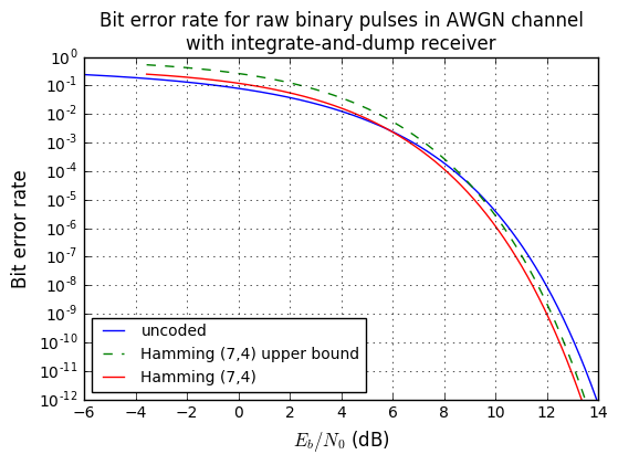
Both the exact calculation and the upper bound are fairly close.
We can do something similar with Reed-Solomon error rates. For an ( (n,k) = (255,255-2t) ) Reed-Solomon code, with transmitted bit error probability ( p ), the error probability per byte is ( q = 1 — (1-p)^8 ), and there are a couple of situations, given the number of byte errors ( v ) per 255-byte block:
- ( v le t ): Reed-Solomon will decode them all correctly, and the number of decoded byte errors is zero.
- ( v > t ): More than ( t ) byte errors: This is the tricky part.
- Best-case estimate: we are lucky and the decoder actually corrects ( t ) errors, leading to ( v-t ) errors.
This is ludicrously optimistic, but it does represent a lower bound on the bit error rate. - Worst-case estimate: we are unlucky and the decoder alters ( t ) values which were correct,
leading to ( v+t ) errors. This is ludicrously pessimistic, but it does represent an upper bound
on the bit error rate. - Empirical estimate: we can actually generate some random samples covering various numbers of errors, and see what a decoder actually does, then use the results to extrapolate a data bit error rate. This will be closer to the expected results, but it can take quite a bit of computation to generate enough random samples and run the decoder algorithm.
- Best-case estimate: we are lucky and the decoder actually corrects ( t ) errors, leading to ( v-t ) errors.
OK, now we’re going to tie all this together and show four graphs:
- Bit error rate of the decoded data (after error correction) vs. raw bit error rate during transmission. This tells us how much the error rate decreases.
- One graph will show large scale error rates.
- Another will show the same data in closer detail.
- Bit error rate of the decoded data vs. ( E_b/N_0 ). This lets us compare bit error rates by how much transmit energy they require to achieve that error rate.
- Effective gain in ( E_b/N_0 ), in decibels, vs. bit error rate of the decoded data.
# Codes under analysis:
class RawAnalyzer(object):
    def bit_error_rate(self, p):
        return p
    @property
    def codename(self):
        return 'uncoded'
    @property
    def rate(self):
        return 1

ha74 = HammingAnalyzer(0b1011)
ha1511 = HammingAnalyzer(0b10011)
analyzers = [RawAnalyzer(), ha74, ha1511,
            ReedSolomonWorstCaseAnalyzer(255,253),
            ReedSolomonBestCaseAnalyzer(255,253),
            ReedSolomonMonteCarloAnalyzer(
              rs.RSCoder(255,253,generator=2,prim=0x11d,fcr=0,c_exp=8))
                 .set_simulation_sample_counts([10]
                    +[10000,5000,2000,1000,1000,1000,1000,1000]
                    +[100]*10),
            ReedSolomonWorstCaseAnalyzer(255,251),
            ReedSolomonBestCaseAnalyzer(255,251),
            ReedSolomonMonteCarloAnalyzer(
              rs.RSCoder(255,251,generator=2,prim=0x11d,fcr=0,c_exp=8))
                 .set_simulation_sample_counts([10]
                    +[10000,5000,2000,1000,1000,1000,1000,1000]
                    +[100]*5),
            ReedSolomonWorstCaseAnalyzer(255,247),
            ReedSolomonBestCaseAnalyzer(255,247),
            ReedSolomonMonteCarloAnalyzer(
              rs.RSCoder(255,247,generator=2,prim=0x11d,fcr=0,c_exp=8))
                 .set_simulation_sample_counts([10]
                    +[10000,5000,2000,1000,1000,1000,1000,1000]
                    +[100]*5),
            ReedSolomonWorstCaseAnalyzer(255,239),
            ReedSolomonBestCaseAnalyzer(255,239),
            ReedSolomonMonteCarloAnalyzer(
              rs.RSCoder(255,239,generator=2,prim=0x11d,fcr=0,c_exp=8))
                 .set_simulation_sample_counts([10]
                    +[10000,5000,2000,1000,1000,1000,1000,1000]),
            ReedSolomonWorstCaseAnalyzer(255,223),
            ReedSolomonBestCaseAnalyzer(255,223),
            ReedSolomonMonteCarloAnalyzer(
              rs.RSCoder(255,223,generator=2,prim=0x11d,fcr=0,c_exp=8))
                 .set_simulation_sample_counts([10]
                    +[5000,2000,1000,500,500,500,500,500]),
            ReedSolomonWorstCaseAnalyzer(255,191),
            ReedSolomonBestCaseAnalyzer(255,191),
            ReedSolomonMonteCarloAnalyzer(
              rs.RSCoder(255,191,generator=2,prim=0x11d,fcr=0,c_exp=8))
                 .set_simulation_sample_counts([10]
                    +[2000,1000,500,500,500,500,500,500]),
            ]
styles = ['k','r','g','b--','b--','b','c--','c--','c',
          'm--','m--','m',
          '#88ff00--','#88ff00--','#88ff00',
          '#ff8800--','#ff8800--','#ff8800',
          '#888888--','#888888--','#888888']
# Sigh. This takes a while.
import time

for analyzer in analyzers:
    if hasattr(analyzer, 'simulate'):
        print "RS(%d,%d)" % (analyzer.n, analyzer.k)
        np.random.seed(123)
        # just to make the Monte Carlo analysis repeatable
        t0 = time.time()
        analyzer.simulate()
        t1 = time.time()
        print "%.2f seconds" % (t1-t0)
RS(255,253)
42.47 seconds
RS(255,251)
44.90 seconds
RS(255,247)
62.66 seconds
RS(255,239)
151.81 seconds
RS(255,223)
197.57 seconds
RS(255,191)
470.05 seconds
ebno_db = np.arange(-6,18,0.02)
ebno = 10**(ebno_db/10)
# Decibels are often confusing.
# dB = 10 log10 x  if x is measured in energy
# dB = 20 log10 x  if x is measured in amplitude.

# Raw bit error probability
p = Q(np.sqrt(2*ebno))
# Binomial distribution -- this is used by the RS Monte Carlo analyzers
pbinom = scipy.stats.binom.pmf(np.atleast_2d(np.arange(800)).T,255*8,p)

error_rates = [analyzer.bit_error_rate(p) for analyzer in analyzers]
colors = [s[:-2] if s.endswith('--') else s for s in styles]
linestyles = ['--' if s.endswith('--') else '-' for s in styles]
def label_for(analyzer):
    codename = analyzer.codename
    if codename.endswith(' worstcase'):
        return None
    elif codename.endswith(' bestcase'):
        return codename[:-8] + 'bounds'
    else:
        return codename

# 1a and 1b. Raw vs. derived probability

for xscale,yscale in [(1e-12,1e-20),(1e-5,1e-8)]:
    fig = plt.figure(figsize=(7,6))
    ax = fig.add_subplot(1,1,1)
    for i, analyzer in enumerate(analyzers):
        p2 = error_rates[i]
        ax.loglog(p, p2,
                  color=colors[i], linestyle=linestyles[i], label=label_for(analyzer))
    ax.set_xlabel('Raw bit error rate')
    ax.set_ylabel('Data bit error rate')
    ax.legend(loc='upper left',fontsize=8, labelspacing=0, handlelength=3)
    ax.grid('on')
    ax.set_title('Code effect on data bit error rate')
    ax.set_xlim(xscale,0.5)
    ax.set_ylim(yscale,1)

# 2. Data error rate vs. Eb/N0
fig = plt.figure(figsize=(7,6))
ax = fig.add_subplot(1,1,1)
for i, analyzer in enumerate(analyzers):
    p2 = error_rates[i]

    ax.semilogy(dBE(ebno/analyzer.rate), p2,
                color=colors[i], linestyle=linestyles[i], label=label_for(analyzer))
ax.set_ylabel('Data bit error rate',fontsize=12)
ax.set_xlabel('$E_b/N_0$ (dB)',fontsize=12)
ax.set_xlim(-6,14)
ax.set_xticks(np.arange(-6,15,2))
ax.set_ylim(1e-12,1)
ax.legend(loc='lower left',fontsize=8, labelspacing=0, handlelength=3)
ax.grid('on')
ax.set_title('Data bit error rate for raw binary pulses in AWGN channeln'
          +'with integrate-and-dump receiver');

# 3. Eb/No gain vs. data error rate
fig = plt.figure(figsize=(7,6))
ax = fig.add_subplot(1,1,1)
for i, analyzer in enumerate(analyzers):
    p2 = error_rates[i]
    ebno_equiv = Qinv(p2)**2/2
    ax.semilogx(p2, dBE(ebno_equiv*analyzer.rate/ebno),
                    color=colors[i], linestyle=linestyles[i], label=label_for(analyzer))
ax.set_xlim(1e-16,0.5)
ax.set_ylim(-8,10)
ax.set_yticks(np.arange(-8,10.1,2))
ax.legend(loc='lower left',fontsize=8, labelspacing=0, handlelength=3)
ax.set_xlabel('Data bit error rate', fontsize=12)
ax.set_ylabel('Gain (dB)', fontsize=12)
ax.grid('on')
ax.set_title('Effective $E_b/N_0$ gain vs data bit error rate');
OK, so what are we looking at here?
The top two graphs show us a few things:
-
At low channel bit error rates (= “raw bit error rate”), the effective data bit error rate can be made much lower. For example, at a ( 10^{-4} ) channel bit error rate, a Hamming (7,4) code can bring the effective data bit error rate down to about ( 10^{-7} ), and an RS(255,239) code can bring the effective data bit error rate down to about ( 10^{-14} ). Much lower, and we don’t have to sacrifice much bandwidth to do it; the code rate of RS(255,239) is 239/255 ≈ 0.9373.
-
At high channel bit error rates, on the other hand, the effective data bit error rate may not be much better, and may even be a little higher than the channel data bit error rate. It looks like on average this could be about a factor of 2 worse, in the cases of low-robustness Reed-Solomon codes like RS(255,253) and RS(255,251).
-
The meaning of “low” and “high” channel bit error rates depends on the coding technique used. Hamming codes are short, so you still see benefits from them at channel bit error rates as high as 0.2, whereas RS(255,251) doesn’t help decrease the error rate unless you have channel bit error rates below 0.0005, and the higher-robustness Reed-Solomon codes like RS(255,223) and RS(255,191) work well up to error rates of about 0.01.
The bottom two graphs show us how this reduction in effective bit error rate trades off against the ( E_b/N_0 ) penalty we get for using up part of our channel capacity for the redundancy of parity bits. (Remember, longer average transmission times per bit times mean that we need a larger ( E_b ) per encoded data bit.)
-
Hamming codes can gain between 0.5-1.5dB of ( E_b/N_0 ) compared to uncoded data, for the same effective data bit error rate.
-
Reed-Solomon codes can gain between 2-10dB of ( E_b/N_0 ) compare to uncoded data, for the same effective data bit error rate.
-
This gain works better at low channel bit error rates; the advantages in ( E_b/N_0 ) compared to uncoded data show up if the data bit error rate is somewhere below the 0.0001 to 0.01 range. Reed-Solomon codes beat Hamming codes once you get below about 0.005 data bit error rate, at least for the high-robustness codes; the Reed-Solomon codes which don’t add much redundancy, like RS(255,253), don’t beat Hamming codes unless the data bit error rate is below ( 10^{-7} ).
-
At high effective bit error rates, the coded messages can have worse performance in terms of ( E_b/N_0 ) for the same effective data bit error rate.
-
We generally want low effective bit error rates anyway; something in the ( 10^{-6} ) to ( 10^{-12} ) range is probably reasonable, depending on the application and how it is affected by errors. Those applications that have other higher-level layers which can handle retries in case of detected errors, can usually get away with bit error rates of ( 10^{-6} ) or even higher. Storage applications, on the other hand, need to keep errors low, because there’s no possible mechanism for retransmission; the only way to deal with it is to add another layer of error correction — which is something that is used in certain applications.
Why Not Use Reed-Solomon Instead of a CRC?
So here’s a question that might come to mind. Consider the following two pairs of cases:
- RS(255,253) vs. a 253-byte packet followed by a 16-bit CRC
- RS(255,251) vs. a 251-byte packet followed by a 32-bit CRC
Within each pair, there is the same overhead, and about the same encoding complexity and memory requirements if a lookup-table-based encoder is used. Decoders that check for the presence of transmission errors are essentially the same complexity as an encoder; it’s only the error-correction step that takes more CPU horsepower.
A CRC can be used to detect errors, but not to correct them. A Reed-Solomon code can be used to detect errors, up to 1 byte error in case of RS(255,253) and two byte errors in case of RS(255,251).
So why shouldn’t we be using Reed-Solomon instead of a CRC?
Well, CRCs are meant for detecting a small number of bit errors with guaranteed certainty. Reed-Solomon codes are designed to handle byte errors, and that means bursts of a byte or two, depending on the code parameters. So the nature of the received noise may make a big difference in terms of which is better. Noise models like AWGN, where the likelihood of any individual bit error is independent of any other, favor bit-error detection techniques; noise models in which multi-bit bursts are common will favor Reed-Solomon.
But the biggest impact is that by allowing error correction, we give up some of our ability to detect errors. I mentioned this toward the end of Part XV. Let’s look at it again.
Dry Imp Net Nrp Nmy
Let’s take a look at our fictitious dry imp net encoding scheme again. Three codewords — dry, imp, and net — and three symbols per word.
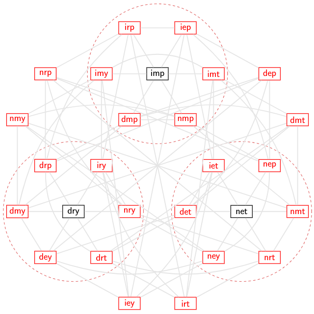
This encoding scheme has a Hamming distance of 3, which means we can detect up to 2 errors or correct up to 1 error.
If we don’t do any error correction, there are only 3 codewords out of 27 possible messages, so our ability to detect invalid messages is very good. The only way we’re going to misinterpret dry as imp or net is if we happen to get the right kind of error to switch from one valid codeword to another, which needs three simultaneous errors.
On the other hand, if we do decide to use error correction, then all of a sudden we have 21 acceptable messages. By “acceptable” I mean a message that is either correct or correctable. If we get a message like dmp that was originally dry, sorry, we’re going to turn it into imp, because that’s the closest codeword. The only unacceptable messages are nrp, nmy, iey, irt, dmt, and dep, which have a minimum distance of 2 to any codeword.
There are a few limited codes — Hamming codes are one of them — which have the property that there are no unacceptable messages. These are called perfect codes, and it means that any received message is either correct or can be corrected to the closest codeword. Here we have to assume that errors are infrequent, and if we do get more errors than we can correct, then we are just going to make an erroneous correction. Oh well.
I looked into this a little bit for Reed-Solomon codes. For ( RS(255,255-2t) ), it looks like ( t=1 ) is close to perfect, and ( t=2 ) isn’t too far away either, but as you start adding more redundancy symbols, the number of uncorrectable messages increases much faster than the number of correctable messages, and these boundaries around each codeword — which are called Hamming spheres, even though they’re more like N-dimensional hypercubes — cover less and less of the message space. Which is good, at least for error detection, because it means we’re more likely to be able to detect errors even if there are more than ( t ) of them.
Below is some data from the Monte Carlo simulations I used to compute bit error rates — this time presented a little differently, showing tables of what happens when there are more than ( t ) errors. Each random error pattern of ( v ) bit errors (and note that this may produce less than ( v ) byte errors, if more than one error occurs in the same byte) can have three outcomes:
CORRECT: the error pattern decodes correctlyFAIL: the decoding step fails, so we don’t change the received message, and the number of received errors stays the sameWORSEN: the error pattern decodes incorrectly, to a different codeword
The table shows the number of samples nsample in each case, and the fraction of those samples that fall into the CORRECT, FAIL, and WORSEN outcomes.
rsanalyzers = [analyzer for analyzer in analyzers
               if isinstance(analyzer, ReedSolomonMonteCarloAnalyzer)]
def summarize_simulation_results(sr):
    shist, fhist = sr
    nfail = sum(fhist)
    nsample = nfail + sum(shist)
    ncorrect = shist[0]
    nworsen = sum(shist[1:])
    return (nsample,
            ncorrect*1.0/nsample,
            nfail*1.0/nsample,
            nworsen*1.0/nsample)
data = [(analyzer.n, analyzer.k, analyzer.t, i+analyzer.t)
       +summarize_simulation_results(sr)
    for analyzer in rsanalyzers
    for i, sr in enumerate(analyzer.simulation_results)
    if i > 0 and i <= 8]
df = pd.DataFrame(data,
            columns='n k t v nsample ncorrect nfail nworsen'.split())
df.set_index(['n','k','t','v'])
| nsample | ncorrect | nfail | nworsen | ||||
|---|---|---|---|---|---|---|---|
| n | k | t | v | ||||
| 255 | 253 | 1 | 2 | 10000 | 0.0029 | 0.1228 | 0.8743 |
| 3 | 5000 | 0.0000 | 0.0000 | 1.0000 | |||
| 4 | 2000 | 0.0000 | 0.0490 | 0.9510 | |||
| 5 | 1000 | 0.0000 | 0.0000 | 1.0000 | |||
| 6 | 1000 | 0.0000 | 0.0130 | 0.9870 | |||
| 7 | 1000 | 0.0000 | 0.0000 | 1.0000 | |||
| 8 | 1000 | 0.0000 | 0.0140 | 0.9860 | |||
| 9 | 1000 | 0.0000 | 0.0000 | 1.0000 | |||
| 251 | 2 | 3 | 10000 | 0.0091 | 0.4998 | 0.4911 | |
| 4 | 5000 | 0.0000 | 0.5036 | 0.4964 | |||
| 5 | 2000 | 0.0000 | 0.5115 | 0.4885 | |||
| 6 | 1000 | 0.0000 | 0.4850 | 0.5150 | |||
| 7 | 1000 | 0.0000 | 0.5110 | 0.4890 | |||
| 8 | 1000 | 0.0000 | 0.4940 | 0.5060 | |||
| 9 | 1000 | 0.0000 | 0.5190 | 0.4810 | |||
| 10 | 1000 | 0.0000 | 0.5070 | 0.4930 | |||
| 247 | 4 | 5 | 10000 | 0.0342 | 0.9288 | 0.0370 | |
| 6 | 5000 | 0.0004 | 0.9628 | 0.0368 | |||
| 7 | 2000 | 0.0000 | 0.9490 | 0.0510 | |||
| 8 | 1000 | 0.0000 | 0.9650 | 0.0350 | |||
| 9 | 1000 | 0.0000 | 0.9710 | 0.0290 | |||
| 10 | 1000 | 0.0000 | 0.9650 | 0.0350 | |||
| 11 | 1000 | 0.0000 | 0.9710 | 0.0290 | |||
| 12 | 1000 | 0.0000 | 0.9610 | 0.0390 | |||
| 239 | 8 | 9 | 10000 | 0.1213 | 0.8787 | 0.0000 | |
| 10 | 5000 | 0.0102 | 0.9898 | 0.0000 | |||
| 11 | 2000 | 0.0000 | 1.0000 | 0.0000 | |||
| 12 | 1000 | 0.0000 | 1.0000 | 0.0000 | |||
| 13 | 1000 | 0.0000 | 1.0000 | 0.0000 | |||
| 14 | 1000 | 0.0000 | 1.0000 | 0.0000 | |||
| 15 | 1000 | 0.0000 | 1.0000 | 0.0000 | |||
| 16 | 1000 | 0.0000 | 1.0000 | 0.0000 | |||
| 223 | 16 | 17 | 5000 | 0.3796 | 0.6204 | 0.0000 | |
| 18 | 2000 | 0.0930 | 0.9070 | 0.0000 | |||
| 19 | 1000 | 0.0200 | 0.9800 | 0.0000 | |||
| 20 | 500 | 0.0020 | 0.9980 | 0.0000 | |||
| 21 | 500 | 0.0000 | 1.0000 | 0.0000 | |||
| 22 | 500 | 0.0000 | 1.0000 | 0.0000 | |||
| 23 | 500 | 0.0000 | 1.0000 | 0.0000 | |||
| 24 | 500 | 0.0000 | 1.0000 | 0.0000 | |||
| 191 | 32 | 33 | 2000 | 0.8490 | 0.1510 | 0.0000 | |
| 34 | 1000 | 0.5580 | 0.4420 | 0.0000 | |||
| 35 | 500 | 0.3160 | 0.6840 | 0.0000 | |||
| 36 | 500 | 0.1700 | 0.8300 | 0.0000 | |||
| 37 | 500 | 0.0720 | 0.9280 | 0.0000 | |||
| 38 | 500 | 0.0220 | 0.9780 | 0.0000 | |||
| 39 | 500 | 0.0080 | 0.9920 | 0.0000 | |||
| 40 | 500 | 0.0020 | 0.9980 | 0.0000 |
The interesting trends here are
- For RS(255,253), with more than 1 error, the outcome is usually
WORSEN. With ( v=2 ) errors we occasionally get a successful correction. Compared to a 16-bit CRC, we risk making errors worse by trying to correct them, so unless we have a system with very low probability of 2 or more errors, we are better off using a 16-bit CRC and not trying to correct errors. - For RS(255,251), with more than 2 errors, the outcome is about a 50-50 split between
FAILandWORSEN. With ( v=3 ) errors we occasionally get a successful correction. Compared to a 32-bit CRC, we risk making errors worse by trying to correct them. It’s not as bad as RS(255,253), but a 50% chance of making things worse if there are three or more errors, makes it more attractive to use a 32-bit CRC. - For RS(255,247), with more than 4 errors, the outcome is usually
FAILwith a small probability ofWORSEN. With ( v=4 ) and ( v=5 ) errors we occasionally get a successful correction. Compared to a 64-bit CRC, now the use of Reed-Solomon becomes much more attractive, at least for packets of length 255 or less. - For RS(255,239) and other decoders with higher ( t ) values, the output almost never is
WORSEN. Probability ofCORRECTbecomes greater even though we are beyond the Hamming bound of at most ( t ) correctible errors. Reed-Solomon is very attractive, but the encoding cost starts to get higher.
These probabilities of a WORSEN outcome are fairly close to their theoretical values, which are just the fraction of all possible messages which are within a Hamming distance of ( t ) of a valid codeword.
For example, if we have RS(255,253), then the last two bytes of valid codewords are completely dependent on the preceding bytes, so the fraction of valid codewords is ( 1/256^2 = 1/65536 ), and the fraction of all possible messages which are within a distance of 1 of those valid codewords is ( frac{1 + 255 times 255}{256^2} approx 0.9922 ). For each codeword we have one message with distance 0 (the codeword itself) and ( 255 times 255 ) messages with distance 1: each of the 255 message bytes can be corrupted with 255 other values.
Or if we have RS(255,251), this fraction becomes ( frac{1 + 255 times 255 + frac{255 times 254}{2} times 255^2}{256^4} approx 0.4903 ).
The general formula for this fraction is
$$rho(t) = 256^{-2t}sumlimits_{j=0}^t {255choose j}255^j$$
which we can graph:
def rscoverage(t):
    y = 0
    p = 1.0/256
    x = 1.0
    for k in xrange(t+1):
        u = x
        for j in xrange(2*t-k):
            if j < k:
                u *= 255.0/256
            else:
                u *= p
        y += u
        x *= (255-k)/256.0
        x /= k+1
    return y

tlist = np.arange(1,21)
fig=plt.figure()
ax=fig.add_subplot(1,1,1)
ax.semilogy(tlist,[rscoverage(t) for t in tlist],'.')
ax.set_title('Fraction of messages in $RS(255,255-2t)$n within distance $t$ of a valid codeword')
ax.set_xlabel('$t$',fontsize=12)
ax.set_ylabel('$\rho$',fontsize=12)
ax.grid('on')
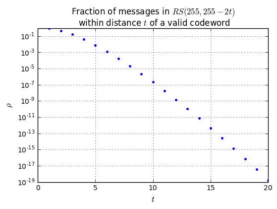
The sweet spot for low-end embedded systems is probably to use Reed-Solomon (255,247), where ( t=4 ). Possibly (255,239), where ( t=8 ). Smaller values of ( t ) allow a table-based implementation with a minimum amount of CPU time and memory; larger values of ( t ) lower the probability of erroneous correction.
But the most important thing is really to understand the behavior of errors in your system:
-
Probability of errors – run some tests and try to figure out the rate of errors without any attempt at error correction. A system with an average error rate of 1 error per ( 10^{6} ) bytes is a much different system to work with, than one that has an average error rate of 1 error per 1000 bytes.
-
Impact of errors – if you’re working with audio data, an error might sound like a brief “pop” in the sound, and this may not be a big deal. If you have a sensor gathering and transmitting data from a once-in-a-lifetime experiment, and losing data can make or break the results, then error correction coding is relatively cheap insurance.
Real-world Applications of Reed-Solomon Codes
Reed-Solomon codes are now in widespread use.
We already talked about the use of Reed-Solomon codes in the Voyager space probes from Uranus and Neptune onwards. They have been supplanted in more recent NASA missions, such as the Mars Reconaissance Encoder by turbo codes, which have higher ( E_b/N_0 ) gain.
Compact discs and DVDs use cross-interleaved Reed-Solomon encoding to increase the robustness against errors even if they show up as scratches impacting large numbers of bits.
Broadband data transmission systems like VDSL2 use Reed-Solomon codes to reduce error rates for a given transmitter energy.
The application I find most interesting is in QR codes, where Reed-Solomon codes are used along with a clever scheme to distribute the data bits spatially over a wide area. This makes them robust to severe data loss errors.

Normally you see QR code images like this:

But they can still be decoded even when part of the information has been corrupted, like this:

or this:

or even this:

I couldn’t find a QR code application that outputs the raw binary bits before decoding, but it would be interesting to see how many errors or erasures these images have. The four levels of error correction in a QR code, L, M, Q, and H, allow up to 30% errors by requiring more bits to encode a given message. The code above is an H-level code, and I kept adding larger and larger disturbances until the decoder was unable to process an image; these are slightly below the failure point, so they are probably in the 25-30% range.
Wrapup
OK! We’ve wandered around the topic of Reed-Solomon codes today, covering a few important points:
- Reed-Solomon codes represent messages as polynomials with coefficients in ( GF(2^m) ), and are often denoted as ( RS(n,k) )
- The Reed-Solomon ( (255,255-2t) ) code is a common subset, representing a codeword as 255 bytes, each byte an element of ( GF(2^8) ). This allows for correction of up to ( t ) errors or ( 2t ) erasures.
- To specify a particular Reed-Solomon code, in addition to knowing ( n ) and ( k ), you need the characteristic polynomial of the symbol field — for ( GF(2^8) ), this is a degree 8 polynomial — and the generator polynomial, which is of the form ( g(x) = (x+lambda^b)(x+lambda^{b+1})(x+lambda^{b+2})ldots (x+lambda^{b+2t-1}) ), where ( b ) is an integer and ( lambda ) is any generating element in ( GF(2^8) ) — meaning that all nonzero elements of ( GF(2^8) ) are expressible as ( lambda^i ) for some integer ( i ) between 0 and 254. The important property of ( g(x) ) is that its roots are ( 2t ) consecutive powers of ( lambda ).
- Algebraically, encoding a message involves expressing it as a polynomial ( M(x) ), computing ( r(x) = x^{2t}M(x) bmod g(x) ) and constructing the codeword ( C_t(x) = x^{2t}M(x) + r(x) )
- In practical terms, we can encode a message using an LFSR where the shift cells contain elements of ( GF(2^8) ) and the LFSR taps are multiplier coefficients in ( GF(2^8) ), each tap corresponding to the corresponding coefficient in the generator polynomial.
- This LFSR approach can be implemented using lookup tables to handle the finite field mathematics
- Decoding takes considerably more processing power, and we didn’t cover the details in this article.
- Shortened Reed-Solomon codes are used by taking an ( (n,k) ) code and using it as an ( (n-l,k-l) ) code, where both transmitter and receiver assume that there are ( l ) implicit zeros at the beginning of the message.
- Calculating bit error rates is a pain. But if you do it right, you will end up with curves of data bit error rate vs. ( E_b/N_0 ), like this graph:
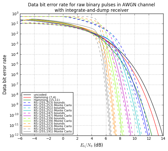
- Higher values of ( t ) reduce the code rate somewhat, but allow for greater gains in ( E_b/N_0 ) for the same data bit error rate. (Or alternatively, much lower data bit error rates for the same amount of signal energy per bit per unit noise.)
-
Use of error correction reduces the robustness to error detection, especially at low values of ( t ), but for ( t > 4 ) or so, the probability of mistakenly correcting more than ( t ) errors to the wrong codeword is very small. The vast majority of the time if there are more than ( t ) errors, the decoder just fails and the number of errors remains unchanged. There are cases with more than ( t ) errors where the decoder would produce a correction to the wrong codeword, but it has a low probability unless the errors are introduced intentionally.
-
Reed-Solomon has lots of applications for reducing the probability of errors: space transmission, storage formats like CDs and DVDs, QR codes, and DSL.
That’s all for today!
Next time we will tackle an interesting problem relating to CRCs.
References
Error-Correcting Codes:
- Gregory Mitchell, ARL-TR-4901: Investigation of Hamming, Reed-Solomon, and Turbo Forward Error Correcting Codes, US Army Research Laboratory, July 2009.
Reed-Solomon / BCH codes:
-
C.K.P. Clarke, WHP031: Reed-Solomon Error Correction, British Broadcasting Corporation, January 2002.
-
William Geisel, NASA Technical Memorandum 102162: Tutorial on Reed-Solomon Error Correction Coding, National Aeronautics and Space Administration, August 1990.
-
John Gill, EE 387 Notes 7: BCH and Reed-Solomon Codes, Stanford University, 2014.
-
Fabrizio Pollara, A Software Simulation Study of a (255,223) Reed-Solomon Encoder-decoder, Jet Propulsion Laboratory, JPL Publication 85-23, April 1985. (This report is interesting because it contains C code for both an encoder and decoder. I have not tried to use either, and it’s nearly unreadable code, using short cryptic identifiers everywhere.)
-
Duke University, CPS296 and notes on decoding.
-
Wikiversity, Reed-Solomon Codes for Coders
-
I. S. Reed and G. Solomon, Polynomial Codes over Certain Finite Fields,
Journal of the Society for Industrial and Applied Mathematics, Volume 8, issue 2, pp. 300–304, June 1960. -
Yasuo Sugiyama, Masao Kasahara, Shigeichi Hirasawa, and Toshihiko Namekawa, A Method for Solving Key Equation for Decoding Goppa Codes, Information and Control
Volume 27, issue 1, January 1975, pp 87-99.
AWGN Channels:
- Dilip Sarwate, ECE 361: Lecture 3: Matched Filters – Part I, 2011. This has the equation for determining the variance of received white noise after it goes through a filter ( h(t) ).
QR Codes:
- Bill Casselman, How to Read QR Symbols Without Your Mobile Telephone, American Mathematical Society, 2013.
© 2018 Jason M. Sachs, all rights reserved.
Error correcting codes are a signal processing technique to correct errors. They are nowadays ubiquitous, such as in communications (mobile phone, internet), data storage and archival (hard drives, optical discs CD/DVD/BluRay, archival tapes), warehouse management (barcodes) and advertisement (QR codes).
Reed–Solomon error correction is a specific type of error correction code. It is one of the oldest but it is still widely used, as it is very well defined and several efficient algorithms are now available under the public domain.
Usually, error correction codes are hidden and most users do not even know about them, nor when they are used. Yet, they are a critical component for some applications to be viable, such as communication or data storage. Indeed, a hard drive that would randomly lose data every few days would be useless, and a phone being able to call only on days with a cloud-less weather would be seldom used. Using error correction codes allows to recover a corrupted message into the full original message.
Barcodes and QR codes are interesting applications to study, as they have the specificity of displaying visually the error correction code, rendering these codes readily accessible to the curious user.
In this essay, we will attempt to introduce the principles of Reed–Solomon codes from the point of view of a programmer rather than a mathematician, which means that we will focus more on the practice than the theory, although we will also explain the theory, but only the necessary knowledge for intuition and implementation. Notable references in the domain will be provided, so that the interested reader can dig deeper into the mathematical theory at will. We will provide real-world examples taken from the popular QR code barcode system as well as working code samples. We chose to use Python for the samples (mainly because it looks pretty and similar to pseudocode), but we will try to explain any non-obvious features for those who are not familiar with it. The mathematics involved is advanced in the sense that it is not usually taught below the university level, but it should be understandable to someone with a good grasp of high-school algebra.
We will first gently introduce the intuitions behind error correction codes principles, then in a second section we will introduce the structural design of QR codes, in other words how information is stored in a QR code and how to read and produce it, and in a third section we will study error correction codes via the implementation of a Reed–Solomon decoder, with a quick introduction of the bigger BCH codes family, in order to reliably read damaged QR codes.
Note for the curious readers that extended information can be found in the appendix and on the discussion page.
Principles of error correction[edit | edit source]
Before detailing the code, it might be useful to understand the intuition behind error correction. Indeed, although error correcting codes may seem daunting mathematically-wise, most of the mathematical operations are high school grade (with the exception of Galois Fields, but which are in fact easy and common for any programmer: it’s simply doing operations on integers modulo a number). However, the complexity of the mathematical ingenuity behind error correction codes hide the quite intuitive goal and mechanisms at play.
Error correcting codes might seem like a difficult mathematical concept, but they are in fact based on an intuitive idea with an ingenious mathematical implementation: let’s make the data structured, in a way that we can «guess» what the data was if it gets corrupted, just by «fixing» the structure. Mathematically-wise, we use polynomials from the Galois Field to implement this structure.
Let’s take a more practical analogy: let’s say you want to communicate messages to someone else, but these messages can get corrupted along the way. The main insight of error correcting codes is that, instead of using a whole dictionary of words, we can use a smaller set of carefully selected words, a «reduced dictionary», so that each word is as different as any other. This way, when we get a message, we just have to lookup inside our reduced dictionary to 1) detect which words are corrupted (as they are not in our reduced dictionary); 2) correct corrupted words by finding the most similar word in our dictionary.
Let’s take a simple example: we have a reduced dictionary with only three words of 4 letters: this, that and corn. Let’s say we receive a corrupted word: co**, where * is an erasure. Since we have only 3 words in our dictionary, we can easily compare our received word with our dictionary to find the word that is the closest. In this case, it’s corn. Thus the missing letters are rn.
Now let’s say we receive the word th**. Here the problem is that we have two words in our dictionary that match the received word: this and that. In this case, we cannot be sure which one it is, and thus we cannot decode. This means that our dictionary is not very good, and we should replace that with another more different word, such as dash to maximize the difference between each word. This difference, or more precisely the minimum number of different letters between any 2 words of our dictionary, is called the maximum Hamming distance of our dictionary. Making sure that any 2 words of the dictionary share a minimum number of letters at the same position is called maximum separability.
The same principle is used for most error correcting codes: we generate a reduced dictionary containing only words with maximum separability (we will detail more how to do that in the third section), and then we communicate only with the words of this reduced dictionary. What Galois Fields provide is the structure (ie, reduced dictionary basis), and Reed–Solomon is a way to automatically create a suitable structure (make a reduced dictionary with maximum separability tailored for a dataset), as well as provide the automated methods to detect and correct errors (ie, lookups in the reduced dictionary). To be more precise, Galois Fields are the structure (thanks to their cyclic nature, the modulo an integer) and Reed–Solomon is the codec (encoder/decoder) based on Galois Fields.
If a word gets corrupted in the communication, that’s no big deal since we can easily fix it by looking inside our dictionary and find the closest word, which is probably the correct one (there is however a chance of choosing a wrong one if the input message is too heavily corrupted, but the probability is very small). Also, the longer our words are, the more separable they are, since more characters can be corrupted without any impact.
The simplest way to generate a dictionary of maximally separable words is to make words longer than they really are.
Let’s take again our example:
   t h i s
   t h a t
   c o r n
Append a unique set of characters so that there are no duplicated characters at any of the appended positions, and add one more word to help with the explanation:
   t h i s a b c d
   t h a t b c d e
   c o r n c d e f
Note that each word in this dictionary differs from every other word by at least 6 characters, so the distance is 6. This allows up to 5 errors in known positions (which are called erasures), or 3 errors in unknown positions, to be corrected.
Assume that 4 erasures occur:
t * * * a b * d
Then a search of the dictionary for the 4 non-erased characters can be done to find the only entry that matches those 4 characters, since the distance is 5. Here it gives: t h i s a b c d
Assume that 2 errors occur as in one of these patterns:
t h o s b c d e
The issue here is the location of the errors is unknown. The erasures might have happened in any 2 positions meaning that there are  or 28 possible sub-sets of 6 characters:
  t h o s b c * *
  t h o s b * d *
  t h o s b * * e
  ...
If we do a dictionary search on each of these sub-sequences, we find that there is only one sub-set that matches 6 characters. t h * * b c d e matches t h a t b c d e.
With these examples, one can see the advantage of redundancy in recovering lost information: redundant characters help you recover your original data. The previous examples show how a crude error correcting scheme could work. Reed–Solomon’s core idea is similar, append redundant data to a message based on Galois Field mathematics. The original error correcting decoder was similar to the error example above, search sub-sets of a received message that correspond to a valid message, and choose the one with the most matches as the corrected message. This isn’t practical for larger messages, so mathematical algorithms were developed to perform error correction in a reasonable time.
QR code structure[edit | edit source]
This section introduces the structure of QR codes, which is how data is stored in a QR code. The information in this section is deliberately incomplete. Only the most common features of the small 21×21 size symbols (also known as version 1) are presented here, but see the appendix for additional information.
Here is a QR symbol that will be used as an example. It consists of dark and light squares, known as modules in the barcoding world. The three square locator patterns in the corners are a visually distinctive feature of QR symbols.

Masking[edit | edit source]
A masking process is used to avoid features in the symbol that might confuse a scanner, such as misleading shapes that look like the locator patterns and large blank areas. Masking inverts certain modules (white becomes black and black becomes white) while leaving others alone.
In the diagram below, the red areas encode format information and use a fixed masking pattern. The data area (in black and white) is masked with a variable pattern. When the code is created, the encoder tries a number of different masks and chooses the one that minimizes undesirable features in the result. The chosen mask pattern is then indicated in the format information so that the decoder knows which one to use. The light gray areas are fixed patterns which do not encode any information. In addition to the obvious locator patterns, there are also timing patterns which contain alternating light and dark modules.

The masking transformation is easily applied (or removed) using the exclusive-or operation (denoted by a caret ^ in many programming languages). The unmasking of the format information is shown below. Reading counter-clockwise around the upper-left locator pattern, we have the following sequence of bits. White modules represent 0 and black modules represent 1.
Input       101101101001011
Mask      ^ 101010000010010
Output      000111101011001
Formatting information[edit | edit source]
There are two identical copies of the formatting information, so that the symbol can still be decoded even if it is damaged. The second copy is broken in two pieces and placed around the other two locators, and is read in a clockwise direction (upwards in the lower-left corner, then left-to-right in the upper-right corner).
The first two bits of formatting information give the error correction level used for the message data. A QR symbol this size contains 26 bytes of information. Some of these are used to store the message and some are used for error correction, as shown in the table below. The left-hand column is simply a name given to that level.
| Error Correction Level | Level Indicator | Error Correction Bytes | Message Data Bytes |
|---|---|---|---|
| L | 01 | 7 | 19 |
| M | 00 | 10 | 16 |
| Q | 11 | 13 | 13 |
| H | 10 | 17 | 9 |
The next three bits of format information select the masking pattern to be used in the data area. The patterns are illustrated below, including the mathematical formula that tells whether a module is black (i and j are the row and column numbers, respectively, and start with 0 in the upper-left hand corner).

The remaining ten bits of formatting information are for correcting errors in the format itself. This will be explained in a later section.
Message data[edit | edit source]
Here is a larger diagram showing the «unmasked» QR code. Different regions of the symbol are indicated, including the boundaries of the message data bytes.

Data bits are read starting from the lower-right corner and moving up the two right-hand columns in a zig-zag pattern. The first three bytes are 01000000 11010010 01110101. The next two columns are read in a downward direction, so the next byte is 01000111. Upon reaching the bottom, the two columns after that are read upward. Proceed in this up-and-down fashion all the way to the left side of the symbol (skipping over the timing pattern where necessary). Here is the complete message in hexadecimal notation.
- Message data bytes: 40 d2 75 47 76 17 32 06 27 26 96 c6 c6 96 70 ec
- Error correction bytes: bc 2a 90 13 6b af ef fd 4b e0
Decoding[edit | edit source]
The final step is to decode the message bytes into something readable. The first four bits indicate how the message is encoded. QR codes use several different encoding schemes, so that different kinds of messages can be stored efficiently. These are summarized in the table below. After the mode indicator is a length field, which tells how many characters are stored. The size of the length field depends on the specific encoding.
| Mode Name | Mode Indicator | Length Bits | Data Bits |
|---|---|---|---|
| Numeric | 0001 | 10 | 10 bits per 3 digits |
| Alphanumeric | 0010 | 9 | 11 bits per 2 characters |
| Byte | 0100 | 8 | 8 bits per character |
| Kanji | 1000 | 8 | 13 bits per character |
(The length field sizes above are valid only for smaller QR codes.)
Our sample message starts with 0100 (hex 4), indicating that there are 8 bits per character. The next 8 bits (hex 0d) are the length field, 13 in decimal notation. The bits after that can be rearranged in bytes representing the actual characters of the messageː 27 54 77 61 73 20 62 72 69 6c 6c 69 67, and additionally 0e c. The first two, hex 27 and 54 are the ASCII codes for apostrophe and T. The whole message is «‘Twas brillig» (from w:Jabberwocky#Lexicon).
After the last of the data bits is another 4-bit mode indicator. It can be different from the first one, allowing different encodings to be mixed within the same QR symbol. When there is no more data to store, the special end-of-message code 0000 is given. (Note that the standard allows the end-of-message code to be omitted if it wouldn’t fit in the available number of data bytes.)
At this point, we know how to decode, or read, a whole QR code. However, in real life conditions, a QR code is rarely whole: usually, it is scanned via a phone’s camera, under potentially poor lighting conditions, or on a scratched surface where part of the QR code was ripped, or on a stained surface, etc.
To make our QR code decoder **reliable**, we need to be able to **correct** errors. The next part of this article will describe how to correct errors, by constructing a BCH decoder, and more specifically a Reed–Solomon decoder.
BCH codes[edit | edit source]
In this section, we introduce a general class of error correction codes: the BCH codes, the parent family of modern Reed–Solomon codes, and the basic detection and correction mechanisms.
The formatting information is encoded with a BCH code which allows a certain number of bit-errors to be detected and corrected. BCH codes are a generalization of Reed–Solomon codes (modern Reed–Solomon codes are BCH codes). In the case of QR codes, the BCH code used for the format information is much simpler than the Reed–Solomon code used for the message data, so it makes sense to start with the BCH code for format information.
BCH error detection[edit | edit source]
The process for checking the encoded information is similar to long division, but uses exclusive-or instead of subtraction. The format code should produce a remainder of zero when it is «divided» by the so-called generator of the code. QR format codes use the generator 10100110111. This process is demonstrated for the format information in the example code (000111101011001) below.
             0001110100110111 )
              000111101011001
               ^ 101001101110
                 010100110111
                ^ 10100110111
                  00000000000
Here is a Python function which implements this calculation.
def qr_check_format(fmt):
   g = 0x537 # = 0b10100110111 in python 2.6+
   for i in range(4,-1,-1):
      if fmt & (1 << (i+10)):
         fmt ^= g << i
   return fmt
Python note: The range function may not be clear to non-Python programmers. It produces a list of numbers counting down from 4 to 0 (the code has «-1» because the interval returned by «range» includes the start but not the end value). In C-derived languages, the for loop might be written as for (i = 4; i >= 0; i--); in Pascal-derived languages, for i := 4 downto 0.
Python note 2: The & operator performs bitwise and, while << is a left bit-shift. This is consistent with C-like languages.
This function can also be used to encode the 5-bit format information.
encoded_format = (format<<10) + qr_check_format(format<<10)
Readers may find it an interesting exercise to generalize this function to divide by different numbers. For example, larger QR codes contain six bits of version information with 12 error correction bits using the generator 1111100100101.
In mathematical formalism, these binary numbers are described as polynomials whose coefficients are integers mod 2. Each bit of the number is a coefficient of one term. For example:
- 10100110111 = 1 x10 + 0 x9 + 1 x8 + 0 x7 + 0 x6 + 1 x5 + 1 x4 + 0 x3 + 1 x2 + 1 x + 1 = x10 + x8 + x5 + x4 + x2 + x + 1
If the remainder produced by qr_check_format is not zero, then the code has been damaged or misread. The next step is to determine which format code is most likely the one that was intended (ie, lookup in our reduced dictionary).
BCH error correction[edit | edit source]
Although sophisticated algorithms for decoding BCH codes exist, they are probably overkill in this case. Since there are only 32 possible format codes, it’s much easier to simply try each one and pick the one that has the smallest number of bits different from the code in question (the number of different bits is known as the Hamming distance). This method of finding the closest code is known as exhaustive search, and is possible only because we have very few codes (a code is a valid message, and here there are only 32, all other binary numbers aren’t correct).
(Note that Reed–Solomon is also based on this principle, but since the number of possible codewords is simply too big, we can’t afford to do an exhaustive search, and that’s why clever but complicated algorithms have been devised, such as Berlekamp-Massey.)
def hamming_weight(x):
   weight = 0
   while x > 0:
      weight += x & 1
      x >>= 1
   return weight

def qr_decode_format(fmt):
   best_fmt = -1
   best_dist = 15
   for test_fmt in range(0,32):
      test_code = (test_fmt<<10) ^ qr_check_format(test_fmt<<10)
      test_dist = hamming_weight(fmt ^ test_code)
      if test_dist < best_dist:
         best_dist = test_dist
         best_fmt = test_fmt
      elif test_dist == best_dist:
         best_fmt = -1
   return best_fmt
The function qr_decode_format returns -1 if the format code could not be unambiguously decoded. This happens when two or more format codes have the same distance from the input.
To run this code in Python, first start IDLE, Python’s integrated development environment. You should see a version message and the interactive input prompt >>>. Open a new window, copy the functions qr_check_format, hamming_weight, and qr_decode_format into it, and save as qr.py. Return to the prompt and type the lines following >>> below.
>>> from qr import *
>>> qr_decode_format(int("000111101011001",2))  # no errors
3
>>> qr_decode_format(int("111111101011001",2))  # 3 bit-errors
3
>>> qr_decode_format(int("111011101011001",2))  # 4 bit-errors
-1
You can also start Python by typing python at a command prompt.
In the next sections, we will study Finite Field Arithmetics and Reed–Solomon code, which is a subtype of BCH codes. The basic idea (ie, using a limited words dictionary with maximum separability) is the same, but since we will encode longer words (256 bytes instead of 2 bytes), with more symbols available (encoded on all 8bits, thus 256 different possible values), we cannot use this naive, exhaustive approach, because it would take way too much time: we need to use cleverer algorithms, and Finite Field mathematics will help us do just that, by giving us a structure.
Finite field arithmetic[edit | edit source]
Introduction to mathematical fields[edit | edit source]
Before discussing the Reed–Solomon codes used for the message, it will be useful to introduce a bit more mathematics.
We’d like to define addition, subtraction, multiplication, and division for 8-bit bytes and always produce 8-bit bytes as a result, so as to avoid any overflow. Naively, we might attempt to use the normal definitions for these operations, and then mod by 256 to keep results from overflowing. And this is exactly what we will be doing, and is what is called a Galois Field 2^8. You can easily imagine why it works for everything, except for division: what is 5/4?
Here’s a brief introduction to Galois Fields: a finite field is a set of numbers, and a field needs to have six properties governing addition, subtraction, multiplication and division: Closure, Associative, Commutative, Distributive, Identity and Inverse. More simply put, using a field allows us to study the relationship between numbers of this field, and apply the result to any other field that follows the same properties. For example, the set of reals ℝ is a field. In other words, mathematical fields studies the structure of a set of numbers.
However, integers ℤ aren’t a field, because as we said above, not all divisions are defined (such as 5/4), which violates multiplicative inverse property (x such that x*4=5 does not exist). One simple way to fix that is to do modulo using a prime number, such as 257, or any positive integer power of a prime number: in this way, we are guaranteed that x*4=5 exists since we will just wrap around. ℤ modulo any prime number is called a Galois Field, and modulo 2 is an extra interesting Galois Field: since an 8-bit string can express a total of 256 = 2^8 values, we say that we use a Galois Field of 2^8, or GF(2^8). In spoken language, 2 is the characteristic of the field, 8 is the exponent, and 256 is the field’s cardinality. More information on finite fields can be found here.
Here we will define the usual mathematical operations that you are used to doing with integers, but adapted to GF(2^8), which is basically doing usual operations but modulo 2^8.
Another way to consider the link between GF(2) and GF(2^8) is to think that GF(2^8) represents a polynomial of 8 binary coefficients. For example, in GF(2^8), 170 is equivalent to 10101010 = 1*x^7 + 0*x^6 + 1*x^5 + 0*x^4 + 1*x^3 + 0*x^2 + 1*x + 0 = x^7 + x^5 + x^3 + x. Both representations are equivalent, it’s just that in the first case, 170, the representation is decimal, and in the other case it’s binary, which can be thought as representing a polynomial by convention (only used in GF(2^p) as explained here). The latter is often the representation used in academic books and in hardware implementations (because of logical gates and registers, which work at the binary level). For a software implementation, the decimal representation can be preferred for clearer and more close-to-the-mathematics code (this is what we will use for the code in this tutorial, except for some examples that will use the binary representation).
In any case, try to not confuse the polynomial representing a single GF(2^p) symbol (each coefficient is a bit/boolean: either 0 or 1), and the polynomial representing a list of GF(2^p) symbols (in this case the polynomial is equivalent to the message+RScode, each coefficient is a value between 0 and 2^p and represent one character of the message+RScode). We will first describe operations on single symbol, then polynomial operations on a list of symbols.
Addition and Subtraction[edit | edit source]
Both addition and subtraction are replaced with exclusive-or in Galois Field base 2. This is logical: addition modulo 2 is exactly like an XOR, and subtraction modulo 2 is exactly the same as addition modulo 2. This is possible because additions and subtractions in this Galois Field are carry-less.
Thinking of our 8-bit values as polynomials with coefficients mod 2:
0101 + 0110 = 0101 - 0110 = 0101 XOR 0110 = 0011
The same way (in binary representation of two single GF(2^8) integers):
- (x2 + 1) + (x2 + x) = 2 x2 + x + 1 = 0 x2 + x + 1 = x + 1
Since (a ^ a) = 0, every number is its own opposite, so (x — y) is the same as (x + y).
Note that in books, you will find additions and subtractions to define some mathematical operations on GF integers, but in practice, you can just XOR (as long as you are in a Galois Field base 2; this is not true in other fields).
Here is the equivalent Python code:
def gf_add(x, y):
    return x ^ y

def gf_sub(x, y):
    return x ^ y # in binary galois field, subtraction is just the same as addition (since we mod 2)
Multiplication[edit | edit source]
Multiplication is likewise based on polynomial multiplication. Simply write the inputs as polynomials and multiply them out using the distributive law as normal. As an example, 10001001 times 00101010 is calculated as follows.
- (x7 + x3 + 1) (x5 + x3 + x) = x7 (x5 + x3 + x) + x3 (x5 + x3 + x) + 1 (x5 + x3 + x)
- = x12 + x10 + 2 x8 + x6 + x5 + x4 + x3 + x
- = x12 + x10 + x6 + x5 + x4 + x3 + x
The same result can be obtained by a modified version of the standard grade-school multiplication procedure, in which we replace addition with exclusive-or.
       10001001
*      00101010
      10001001
^   10001001
^ 10001001
  1010001111010
Note: the XOR multiplication here is carry-less! If you do it with-carry, you will get the wrong result 1011001111010 with the extra term x9 instead of the correct result 1010001111010.
Here is a Python function which implements this polynomial multiplication on single GF(2^8) integers.
Note: this function (and some other functions below) use a lot of bitwise operators such as >> and <<, because they are both faster and more concise to do what we want to do. These operators are available in most languages, they are not specific to Python, and you can get more information about them here.
def cl_mul(x,y):
    '''Bitwise carry-less multiplication on integers'''
    z = 0
    i = 0
    while (y>>i) > 0:
        if y & (1<<i):
            z ^= x<<i
        i += 1
    return z
Of course, the result no longer fits in an 8-bit byte (in this example, it is 13 bits long), so we need to perform one more step before we are finished. The result is reduced modulo 100011101 (the choice of this number is explained below the code), using the long division process described previously. In this instance, this is called «modular reduction», because basically what we do is that we divide and keep only the remainder, using a modulo. This produces the final answer 11000011 in our example.
  1010001111010
^ 100011101
  0010110101010
  ^ 100011101
    00111011110
    ^ 100011101
      011000011
Here is the Python code to do the whole Galois Field multiplication with modular reduction:
def gf_mult_noLUT(x, y, prim=0):
    '''Multiplication in Galois Fields without using a precomputed look-up table (and thus it's slower)
    by using the standard carry-less multiplication + modular reduction using an irreducible prime polynomial'''

    ### Define bitwise carry-less operations as inner functions ###
    def cl_mult(x,y):
        '''Bitwise carry-less multiplication on integers'''
        z = 0
        i = 0
        while (y>>i) > 0:
            if y & (1<<i):
                z ^= x<<i
            i += 1
        return z

    def bit_length(n):
        '''Compute the position of the most significant bit (1) of an integer. Equivalent to int.bit_length()'''
        bits = 0
        while n >> bits: bits += 1
        return bits

    def cl_div(dividend, divisor=None):
        '''Bitwise carry-less long division on integers and returns the remainder'''
        # Compute the position of the most significant bit for each integers
        dl1 = bit_length(dividend)
        dl2 = bit_length(divisor)
        # If the dividend is smaller than the divisor, just exit
        if dl1 < dl2:
            return dividend
        # Else, align the most significant 1 of the divisor to the most significant 1 of the dividend (by shifting the divisor)
        for i in range(dl1-dl2,-1,-1):
            # Check that the dividend is divisible (useless for the first iteration but important for the next ones)
            if dividend & (1 << i+dl2-1):
                # If divisible, then shift the divisor to align the most significant bits and XOR (carry-less subtraction)
                dividend ^= divisor << i
        return dividend

    ### Main GF multiplication routine ###

    # Multiply the gf numbers
    result = cl_mult(x,y)
    # Then do a modular reduction (ie, remainder from the division) with an irreducible primitive polynomial so that it stays inside GF bounds
    if prim > 0:
        result = cl_div(result, prim)

    return result
Result:
>>> a = 0b10001001
>>> b = 0b00101010
>>> print bin(gf_mult_noLUT(a, b, 0)) # multiplication only
0b1010001111010
>>> print bin(gf_mult_noLUT(a, b, 0x11d)) # multiplication + modular reduction
0b11000011
Why mod 100011101 (in hexadecimal: 0x11d)? The mathematics is a little complicated here, but in short, 100011101 represents an 8th degree polynomial which is «irreducible» (meaning it can’t be represented as the product of two smaller polynomials). This number is called a primitive polynomial or irreducible polynomial, or prime polynomial (we will mainly use this latter name for the rest of this tutorial). This is necessary for division to be well-behaved, which is to stay in the limits of the Galois Field, but without duplicating values. There are other numbers we could have chosen, but they’re all essentially the same, and 100011101 (0x11d) is a common primitive polynomial for Reed–Solomon codes. If you are curious to know how to generate those prime polynomials, please see the appendix.
Additional infos on the prime polynomial (you can skip): What is a prime polynomial? It is the equivalent of a prime number, but in the Galois Field. Remember that a Galois Field uses values that are multiples of 2 as the generator. Of course, a prime number cannot be a multiple of two in standard arithmetics, but in a Galois Field it is possible. Why do we need a prime polynomial? Because to stay in the bound of the field, we need to compute the modulo of any value above the Galois Field. Why don’t we just modulo with the Galois Field size? Because we will end up with lots of duplicate values, and we want to have as many unique values as possible in the field, so that a number always has one and only projection when doing a modulo or a XOR with the prime polynomial.
Note for the interested reader: as an example of what you can achieve with clever algorithms, here is another way to achieve multiplication of GF numbers in a more concise and faster way, using the Russian Peasant Multiplication algorithm:
def gf_mult_noLUT(x, y, prim=0, field_charac_full=256, carryless=True):
    '''Galois Field integer multiplication using Russian Peasant Multiplication algorithm (faster than the standard multiplication + modular reduction).
    If prim is 0 and carryless=False, then the function produces the result for a standard integers multiplication (no carry-less arithmetics nor modular reduction).'''
    r = 0
    while y: # while y is above 0
        if y & 1: r = r ^ x if carryless else r + x # y is odd, then add the corresponding x to r (the sum of all x's corresponding to odd y's will give the final product). Note that since we're in GF(2), the addition is in fact an XOR (very important because in GF(2) the multiplication and additions are carry-less, thus it changes the result!).
        y = y >> 1 # equivalent to y // 2
        x = x << 1 # equivalent to x*2
        if prim > 0 and x & field_charac_full: x = x ^ prim # GF modulo: if x >= 256 then apply modular reduction using the primitive polynomial (we just subtract, but since the primitive number can be above 256 then we directly XOR).

    return r
Note that using this last function with parameters prim=0 and carryless=False will return the result for a standard integers multiplication (and thus you can see the difference between carryless and with-carry addition and its impact on multiplication).
Multiplication with logarithms[edit | edit source]
The procedure described above is not the most convenient way to implement Galois field multiplication. Multiplying two numbers takes up to eight iterations of the multiplication loop, followed by up to eight iterations of the division loop. However, we can multiply with no looping by using lookup tables. One solution would be to construct the entire multiplication table in memory, but that would require a bulky 64k table. The solution described below is much more compact.
First, notice that it is particularly easy to multiply by 2=00000010 (by convention, this number is referred to as α or the generator number): simply left-shift by one place, then exclusive-or with the modulus 100011101 if necessary (why xor is sufficient for taking the mod in this case is an exercise left to the reader). Here are the first few powers of α.
| α0 = 00000001 | α4 = 00010000 | α8 = 00011101 | α12 = 11001101 |
| α1 = 00000010 | α5 = 00100000 | α9 = 00111010 | α13 = 10000111 |
| α2 = 00000100 | α6 = 01000000 | α10 = 01110100 | α14 = 00010011 |
| α3 = 00001000 | α7 = 10000000 | α11 = 11101000 | α15 = 00100110 |
If this table is continued in the same fashion, the powers of α do not repeat themselves until α255 = 00000001. Thus, every element of the field except zero is equal to some power of α. The element α, that we define, is known as a primitive element or generator of the Galois field.
This observation suggests another way to implement multiplication: by adding the exponents of α.
- 10001001 * 00101010 = α74 * α142 = α74 + 142 = α216 = 11000011
The problem is, how do we find the power of α that corresponds to 10001001? This is known as the discrete logarithm problem, and no efficient general solution is known. However, since there are only 256 elements in this field, we can easily construct a table of logarithms. While we’re at it, a corresponding table of antilogs (exponentials) will also be useful. More mathematical information about this trick can be found here.
gf_exp = [0] * 512 # Create list of 512 elements. In Python 2.6+, consider using bytearray
gf_log = [0] * 256

def init_tables(prim=0x11d):
    '''Precompute the logarithm and anti-log tables for faster computation later, using the provided primitive polynomial.'''
    # prim is the primitive (binary) polynomial. Since it's a polynomial in the binary sense,
    # it's only in fact a single galois field value between 0 and 255, and not a list of gf values.
    global gf_exp, gf_log
    gf_exp = [0] * 512 # anti-log (exponential) table
    gf_log = [0] * 256 # log table
    # For each possible value in the galois field 2^8, we will pre-compute the logarithm and anti-logarithm (exponential) of this value
    x = 1
    for i in range(0, 255):
        gf_exp[i] = x # compute anti-log for this value and store it in a table
        gf_log[x] = i # compute log at the same time
        x = gf_mult_noLUT(x, 2, prim)

        # If you use only generator==2 or a power of 2, you can use the following which is faster than gf_mult_noLUT():
        #x <<= 1 # multiply by 2 (change 1 by another number y to multiply by a power of 2^y)
        #if x & 0x100: # similar to x >= 256, but a lot faster (because 0x100 == 256)
            #x ^= prim # substract the primary polynomial to the current value (instead of 255, so that we get a unique set made of coprime numbers), this is the core of the tables generation

    # Optimization: double the size of the anti-log table so that we don't need to mod 255 to
    # stay inside the bounds (because we will mainly use this table for the multiplication of two GF numbers, no more).
    for i in range(255, 512):
        gf_exp[i] = gf_exp[i - 255]
    return [gf_log, gf_exp]
Python note: The range operator’s upper bound is exclusive, so gf_exp[255] is not set twice by the above.
The gf_exp table is oversized in order to simplify the multiplication function. This way, we don’t have to check to make sure that gf_log[x] + gf_log[y] is within the table size.
def gf_mul(x,y):
    if x==0 or y==0:
        return 0
    return gf_exp[gf_log[x] + gf_log[y]] # should be gf_exp[(gf_log[x]+gf_log[y])%255] if gf_exp wasn't oversized
Division[edit | edit source]
Another advantage of the logarithm table approach is that it allows us to define division using the difference of logarithms. In the code below, 255 is added to make sure the difference isn’t negative.
def gf_div(x,y):
    if y==0:
        raise ZeroDivisionError()
    if x==0:
        return 0
    return gf_exp[(gf_log[x] + 255 - gf_log[y]) % 255]
Python note: The raise statement throws an exception and aborts execution of the gf_div function.
With this definition of division, gf_div(gf_mul(x,y),y)==x for any x and any nonzero y.
Readers who are more advanced programmers may find it interesting to write a class encapsulating Galois field arithmetic. Operator overloading can be used to replace calls to gf_mul and gf_div with the familiar operators * and /, but this can lead to confusion as to exactly what type of operation is being performed. Certain details can be generalized in ways that would make the class more widely useful. For example, Aztec codes use five different Galois fields with element sizes ranging from 4 to 12 bits.
Power and Inverse[edit | edit source]
The logarithm table approach will once again simplify and speed up our calculations when computing the power and the inverse:
def gf_pow(x, power):
    return gf_exp[(gf_log[x] * power) % 255]

def gf_inverse(x):
    return gf_exp[255 - gf_log[x]] # gf_inverse(x) == gf_div(1, x)
Polynomials[edit | edit source]
Before moving on to Reed–Solomon codes, we need to define several operations on polynomials whose coefficients are Galois field elements. This is a potential source of confusion, since the elements themselves are described as polynomials; my advice is not to think about it too much. Adding to the confusion is the fact that x is still used as the placeholder. This x has nothing to do with the x mentioned previously, so don’t mix them up.
The binary notation used previously for Galois field elements starts to become inconveniently bulky at this point, so I will switch to hexadecimal instead.
- 00000001 x4 + 00001111 x3 + 00110110 x2 + 01111000 x + 01000000 = 01 x4 + 0f x3 + 36 x2 + 78 x + 40
In Python, polynomials will be represented by a list of numbers in descending order of powers of x, so the polynomial above becomes [ 0x01, 0x0f, 0x36, 0x78, 0x40 ]. (The reverse order could have been used instead; both choices have their advantages and disadvantages.)
The first function multiplies a polynomial by a scalar.
def gf_poly_scale(p,x):
    r = [0] * len(p)
    for i in range(0, len(p)):
        r[i] = gf_mul(p[i], x)
    return r
Note to Python programmers: This function is not written in a «pythonic» style. It could be expressed quite elegantly as a list comprehension, but I have limited myself to language features that are easier to translate to other programming languages.
This function «adds» two polynomials (using exclusive-or, as usual).
def gf_poly_add(p,q):
    r = [0] * max(len(p),len(q))
    for i in range(0,len(p)):
        r[i+len(r)-len(p)] = p[i]
    for i in range(0,len(q)):
        r[i+len(r)-len(q)] ^= q[i]
    return r
The next function multiplies two polynomials.
def gf_poly_mul(p,q):
    '''Multiply two polynomials, inside Galois Field'''
    # Pre-allocate the result array
    r = [0] * (len(p)+len(q)-1)
    # Compute the polynomial multiplication (just like the outer product of two vectors,
    # we multiply each coefficients of p with all coefficients of q)
    for j in range(0, len(q)):
        for i in range(0, len(p)):
            r[i+j] ^= gf_mul(p[i], q[j]) # equivalent to: r[i + j] = gf_add(r[i+j], gf_mul(p[i], q[j]))
                                                         # -- you can see it's your usual polynomial multiplication
    return r
Finally, we need a function to evaluate a polynomial at a particular value of x, producing a scalar result. Horner’s method is used to avoid explicitly calculating powers of x. Horner’s method works by factorizing consecutively the terms, so that we always deal with x^1, iteratively, avoiding the computation of higher degree terms:
- 01 x4 + 0f x3 + 36 x2 + 78 x + 40 = (((01 x + 0f) x + 36) x + 78) x + 40
def gf_poly_eval(poly, x):
    '''Evaluates a polynomial in GF(2^p) given the value for x. This is based on Horner's scheme for maximum efficiency.'''
    y = poly[0]
    for i in range(1, len(poly)):
        y = gf_mul(y, x) ^ poly[i]
    return y
There’s still one missing polynomial operation that we will need: polynomial division. This is more complicated than the other operations on polynomial, so we will study it in the next chapter, along with Reed–Solomon encoding.
Reed–Solomon codes[edit | edit source]
Now that the preliminaries are out of the way, we are ready to begin looking at Reed–Solomon codes.
Insight of the coding theory[edit | edit source]
But first, why did we have to learn about finite fields and polynomials? Because this is the main insight of error-correcting codes like Reed–Solomon: instead of just seeing a message as a series of (ASCII) numbers, we see it as a polynomial following the very well-defined rules of finite field arithmetic. In other words, by representing the data using polynomials and finite fields arithmetic, we added a structure to the data. The values of the message are still the same, but this conceptual structure now allows us to operate on the message, on its characters values, using well defined mathematical rules. This structure, that we always know because it’s outside and independent of the data, is what allows us to repair a corrupted message.
Thus, even if in your code implementation you may choose to not explicitly represent the polynomials and the finite field arithmetic, these notions are essential for the error-correcting codes to work, and you will find these notions to underlie (even if implicitly) any implementation.
And now we will put these notions into practice!
RS encoding[edit | edit source]
Encoding outline[edit | edit source]
Like BCH codes, Reed–Solomon codes are encoded by dividing the polynomial representing the message by an irreducible generator polynomial, and then the remainder is the RS code, which we will just append to the original message.
Why? We previously said that the principle behind BCH codes, and most other error correcting codes, is to use a reduced dictionary with very different words as to maximize the distance between words, and that longer words have greater distance: here it’s the same principle, first because we lengthen the original message with additional symbols (the remainder) which raises the distance, and secondly because the remainder is almost unique (thanks to the carefully designed irreducible generator polynomial), so that it can be exploited by clever algorithms to deduce parts of the original message.
To summary, with an approximated analogy to encryption: our generator polynomial is our encoding dictionary, and polynomial division is the operator to convert our message using the dictionary (the generator polynomial) into a RS code.
Exception management[edit | edit source]
To manage errors and cases where we can’t correct a message, we will display a meaningful error message, by raising an exception. We will make our own custom exception so that users can easily catch and manage them:
class ReedSolomonError(Exception):
    pass
To display an error by raising our custom exception, we can then simply do the following:
raise ReedSolomonError("Some error message")
And you can easily catch this exception to manage it by using a try/except block:
try:
    raise ReedSolomonError("Some error message")
except ReedSolomonError as e:
    pass # do something here
RS generator polynomial[edit | edit source]
Reed–Solomon codes use a generator polynomial similar to BCH codes (not to be confused with the generator number alpha). The generator is the product of factors (x — αn), starting with n=0 for QR codes.
For example:
g4(x) = (x — α0) (x — α1) (x — α2) (x — α3)
The same as (x + ai) because of GF(2^8).
g4(x) = x4 — (α3+α2+α1+α0) x3 + ((α0+α1) (α2+α3)+(α5+α1)) x2 + (α6+α5+α4+α3) x +α6
g4(x) = x4 — (α3+α2+α1+α0) x3 + (α2+α3+α3+α4+α5+α1) x2 + (α6+α5+α4+α3) x +α6
g4(x) = x4 — (α3+α2+α1+α0) x3 + (α5+α4+α2+α1) x2 + (α6+α5+α4+α3) x +α6
g4(x) = 01 x4 + 0f x3 + 36 x2 + 78 x + 40
Here is a function that computes the generator polynomial for a given number of error correction symbols.
def rs_generator_poly(nsym):
    '''Generate an irreducible generator polynomial (necessary to encode a message into Reed-Solomon)'''
    g = [1]
    for i in range(0, nsym):
        g = gf_poly_mul(g, [1, gf_pow(2, i)])
    return g
This function is somewhat inefficient in that it allocates successively larger arrays for g. While this is unlikely to be a performance problem in practice, readers who are inveterate optimizers may find it interesting to rewrite it so that g is only allocated once, or you can compute once and memorize g since it is fixed for a given nsym, so you can reuse g.
Polynomial division[edit | edit source]
Several algorithms for polynomial division exist, the simplest one that is often taught in elementary school is long division. This example shows the calculation for the message 12 34 56.
                             12 da df
01 0f 36 78 40 ) 12 34 56 00 00 00 00
               ^ 12 ee 2b 23 f4
                    da 7d 23 f4 00
                  ^ da a2 85 79 84
                       df a6 8d 84 00
                     ^ df 91 6b fc d9
                          37 e6 78 d9
Note: The concepts of polynomial long division apply, but there are a few important differences: When computing the resulting terms/coefficients that will be Galois Field subtracted from the divisor, bitwise carryless multiplication is performed and the result «bitstream» is XORed from the first encountered MSB with the chosen primitive polynomial until the answer is less than the Galois Field value, in this case, 256. The XOR «subtractions» are then performed as usual.
To illustrate the method for one operation (0x12 * 0x36):
    00010010 ( 12 )
  x 00110110 ( 36 )
   00110110
00110110
001100001100
 ^100011101   <-- XOR with primitive polynomial value (11D)...
000100110110
  ^100011101  <-- ...until answer is less than 256.
    00101011
       2   b
The remainder is concatenated with the message, so the encoded message is 12 34 56 37 e6 78 d9.
However, long division is quite slow as it requires a lot of recursive iterations to terminate. More efficient strategies can be devised, such as using synthetic division (also called Horner’s method, a good tutorial video can be found on Khan Academy). Here is a function that implements extended synthetic division of GF(2^p) polynomials (extended because the divisor is a polynomial instead of a monomial):
def gf_poly_div(dividend, divisor):
    '''Fast polynomial division by using Extended Synthetic Division and optimized for GF(2^p) computations
    (doesn't work with standard polynomials outside of this galois field, see the Wikipedia article for generic algorithm).'''
    # CAUTION: this function expects polynomials to follow the opposite convention at decoding:
    # the terms must go from the biggest to lowest degree (while most other functions here expect
    # a list from lowest to biggest degree). eg: 1 + 2x + 5x^2 = [5, 2, 1], NOT [1, 2, 5]

    msg_out = list(dividend) # Copy the dividend
    #normalizer = divisor[0] # precomputing for performance
    for i in range(0, len(dividend) - (len(divisor)-1)):
        #msg_out[i] /= normalizer # for general polynomial division (when polynomials are non-monic), the usual way of using
                                  # synthetic division is to divide the divisor g(x) with its leading coefficient, but not needed here.
        coef = msg_out[i] # precaching
        if coef != 0: # log(0) is undefined, so we need to avoid that case explicitly (and it's also a good optimization).
            for j in range(1, len(divisor)): # in synthetic division, we always skip the first coefficient of the divisior,
                                              # because it's only used to normalize the dividend coefficient
                if divisor[j] != 0: # log(0) is undefined
                    msg_out[i + j] ^= gf_mul(divisor[j], coef) # equivalent to the more mathematically correct
                                                               # (but xoring directly is faster): msg_out[i + j] += -divisor[j] * coef

    # The resulting msg_out contains both the quotient and the remainder, the remainder being the size of the divisor
    # (the remainder has necessarily the same degree as the divisor -- not length but degree == length-1 -- since it's
    # what we couldn't divide from the dividend), so we compute the index where this separation is, and return the quotient and remainder.
    separator = -(len(divisor)-1)
    return msg_out[:separator], msg_out[separator:] # return quotient, remainder.
Encoding main function[edit | edit source]
And now, here’s how to encode a message to get its RS code:
def rs_encode_msg(msg_in, nsym):
    '''Reed-Solomon main encoding function'''
    gen = rs_generator_poly(nsym)

    # Pad the message, then divide it by the irreducible generator polynomial
    _, remainder = gf_poly_div(msg_in + [0] * (len(gen)-1), gen)
    # The remainder is our RS code! Just append it to our original message to get our full codeword (this represents a polynomial of max 256 terms)
    msg_out = msg_in + remainder
    # Return the codeword
    return msg_out
Simple, isn’t it? Encoding is in fact the easiest part in Reed–Solomon, and it’s always the same approach (polynomial division). Decoding is the tough part of Reed–Solomon, and you will find a lot of different algorithms depending on your needs, but we will touch on that later on.
This function is quite fast, but since encoding is quite critical, here is an enhanced encoding function that inlines the polynomial synthetic division, which is the form that you will most often find in Reed–Solomon software libraries:
def rs_encode_msg(msg_in, nsym):
    '''Reed-Solomon main encoding function, using polynomial division (algorithm Extended Synthetic Division)'''
    if (len(msg_in) + nsym) > 255: raise ValueError("Message is too long (%i when max is 255)" % (len(msg_in)+nsym))
    gen = rs_generator_poly(nsym)
    # Init msg_out with the values inside msg_in and pad with len(gen)-1 bytes (which is the number of ecc symbols).
    msg_out = [0] * (len(msg_in) + len(gen)-1)
    # Initializing the Synthetic Division with the dividend (= input message polynomial)
    msg_out[:len(msg_in)] = msg_in

    # Synthetic division main loop
    for i in range(len(msg_in)):
        # Note that it's msg_out here, not msg_in. Thus, we reuse the updated value at each iteration
        # (this is how Synthetic Division works: instead of storing in a temporary register the intermediate values,
        # we directly commit them to the output).
        coef = msg_out[i]

        # log(0) is undefined, so we need to manually check for this case. There's no need to check
        # the divisor here because we know it can't be 0 since we generated it.
        if coef != 0:
            # in synthetic division, we always skip the first coefficient of the divisior, because it's only used to normalize the dividend coefficient (which is here useless since the divisor, the generator polynomial, is always monic)
            for j in range(1, len(gen)):
                msg_out[i+j] ^= gf_mul(gen[j], coef) # equivalent to msg_out[i+j] += gf_mul(gen[j], coef)

    # At this point, the Extended Synthetic Divison is done, msg_out contains the quotient in msg_out[:len(msg_in)]
    # and the remainder in msg_out[len(msg_in):]. Here for RS encoding, we don't need the quotient but only the remainder
    # (which represents the RS code), so we can just overwrite the quotient with the input message, so that we get
    # our complete codeword composed of the message + code.
    msg_out[:len(msg_in)] = msg_in

    return msg_out
This algorithm is faster, but it’s still quite slow for practical use, particularly in Python. There are some ways to optimize the speed by using various tricks, such as inlining (instead of gf_mul, replace by the operation to avoid a call), by precomputing (the logarithm of gen and of coef, or even by generating a multiplication table – but it seems the latter does not work well in Python), by using statically typed constructs (assign gf_log and gf_exp to array.array('i', [...])), by using memoryviews (like by changing all your lists to bytearrays), by running it with PyPy, or by converting the algorithm into a Cython or a C extension[1].
This example shows the encode function applied to the message in the sample QR code introduced earlier. The calculated error correction symbols (on the second line) match the values decoded from the QR code.
>>> msg_in = [ 0x40, 0xd2, 0x75, 0x47, 0x76, 0x17, 0x32, 0x06,
...            0x27, 0x26, 0x96, 0xc6, 0xc6, 0x96, 0x70, 0xec ]
>>> msg = rs_encode_msg(msg_in, 10)
>>> for i in range(0,len(msg)):
...    print(hex(msg[i]), end=' ')
...
0x40 0xd2 0x75 0x47 0x76 0x17 0x32 0x6 0x27 0x26 0x96 0xc6 0xc6 0x96 0x70 0xec
0xbc 0x2a 0x90 0x13 0x6b 0xaf 0xef 0xfd 0x4b 0xe0
Python version note: The syntax for the print function has changed, and this example uses the Python 3.0+ version. In previous versions of Python (particularly Python 2.x), replace the print line with print hex(msg[i]), (including the final comma) and range by xrange.
RS decoding[edit | edit source]
Decoding outline[edit | edit source]
Reed–Solomon decoding is the process that, from a potentially corrupted message and a RS code, returns a corrected message. In other words, decoding is the process of repairing your message using the previously computed RS code.
Although there is only one way to encode a message with Reed–Solomon, there are lots of different ways to decode them, and thus there are a lot of different decoding algorithms.
However, we can generally outline the decoding process in 5 steps[2][3]:
- Compute the syndromes polynomial. This allows us to analyze what characters are in error using Berlekamp-Massey (or another algorithm), and also to quickly check if the input message is corrupted at all.
- Compute the erasure/error locator polynomial (from the syndromes). This is computed by Berlekamp-Massey, and is a detector that will tell us exactly what characters are corrupted.
- Compute the erasure/error evaluator polynomial (from the syndromes and erasure/error locator polynomial). Necessary to evaluate how much the characters were tampered (ie, helps to compute the magnitude).
- Compute the erasure/error magnitude polynomial (from all 3 polynomials above): this polynomial can also be called the corruption polynomial, since in fact it exactly stores the values that need to be subtracted from the received message to get the original, correct message (i.e., with correct values for erased characters). In other words, at this point, we extracted the noise and stored it in this polynomial, and we just have to remove this noise from the input message to repair it.
- Repair the input message simply by subtracting the magnitude polynomial from the input message.
We will describe each of those five steps below.
In addition, decoders can also be classified by the type of error they can repair: erasures (we know the location of the corrupted characters but not the magnitude), errors (we ignore both the location and magnitude), or a mix of errors-and-erasures. We will describe how to support all of these.
Syndrome calculation[edit | edit source]
Decoding a Reed–Solomon message involves several steps. The first step is to calculate the «syndrome» of the message. Treat the message as a polynomial and evaluate it at α0, α1, α2, …, αn. Since these are the zeros of the generator polynomial, the result should be zero if the scanned message is undamaged (this can be used to check if the message is corrupted, and after correction of a corrupted message if the message was completely repaired). If not, the syndromes contain all the information necessary to determine the correction that should be made. It is simple to write a function to calculate the syndromes.
def rs_calc_syndromes(msg, nsym):
    '''Given the received codeword msg and the number of error correcting symbols (nsym), computes the syndromes polynomial.
    Mathematically, it's essentially equivalent to a Fourrier Transform (Chien search being the inverse).
    '''
    # Note the "[0] +" : we add a 0 coefficient for the lowest degree (the constant). This effectively shifts the syndrome, and will shift every computations depending on the syndromes (such as the errors locator polynomial, errors evaluator polynomial, etc. but not the errors positions).
    # This is not necessary, you can adapt subsequent computations to start from 0 instead of skipping the first iteration (ie, the often seen range(1, n-k+1)),
    synd = [0] * nsym
    for i in range(0, nsym):
        synd[i] = gf_poly_eval(msg, gf_pow(2,i))
    return [0] + synd # pad with one 0 for mathematical precision (else we can end up with weird calculations sometimes)
Continuing the example, we see that the syndromes of the original codeword without any corruption are indeed zero. Introducing a corruption of at least one character into the message or its RS code gives nonzero syndromes.
>>> synd = rs_calc_syndromes(msg, 10)
>>> print(synd)
[0, 0, 0, 0, 0, 0, 0, 0, 0, 0, 0] # not corrupted message = all 0 syndromes
>>> msg[0] = 0  # deliberately damage the message
>>> synd = rs_calc_syndromes(msg, 10)
>>> print(synd)
[0, 64, 192, 93, 231, 52, 92, 228, 49, 83, 245] # when corrupted, the syndromes will be non zero
Here is the code to automate this checking:
def rs_check(msg, nsym):
    '''Returns true if the message + ecc has no error or false otherwise (may not always catch a wrong decoding or a wrong message, particularly if there are too many errors -- above the Singleton bound --, but it usually does)'''
    return ( max(rs_calc_syndromes(msg, nsym)) == 0 )
Erasure correction[edit | edit source]
It is simplest to correct mistakes in the code if the locations of the mistakes are already known. This is known as erasure correction. It is possible to correct one erased symbol (ie, character) for each error-correction symbol added to the code. If the error locations are not known, two EC symbols are needed for each symbol error (so you can correct twice less errors than erasures). This makes erasure correction useful in practice if part of the QR code being scanned is covered or physically torn away. It may be difficult for a scanner to determine that this has happened, though, so not all QR code scanners can perform erasure correction.
Now that we already have the syndromes, we need to compute the locator polynomial. This is easy:
def rs_find_errata_locator(e_pos):
    '''Compute the erasures/errors/errata locator polynomial from the erasures/errors/errata positions
       (the positions must be relative to the x coefficient, eg: "hello worldxxxxxxxxx" is tampered to "h_ll_ worldxxxxxxxxx"
       with xxxxxxxxx being the ecc of length n-k=9, here the string positions are [1, 4], but the coefficients are reversed
       since the ecc characters are placed as the first coefficients of the polynomial, thus the coefficients of the
       erased characters are n-1 - [1, 4] = [18, 15] = erasures_loc to be specified as an argument.'''

    e_loc = [1] # just to init because we will multiply, so it must be 1 so that the multiplication starts correctly without nulling any term
    # erasures_loc = product(1 - x*alpha**i) for i in erasures_pos and where alpha is the alpha chosen to evaluate polynomials.
    for i in e_pos:
        e_loc = gf_poly_mul( e_loc, gf_poly_add([1], [gf_pow(2, i), 0]) )
    return e_loc
Next, computing the erasure/error evaluator polynomial from the locator polynomial is easy, it’s simply a polynomial multiplication followed by a polynomial division (that you can replace by a list slicing because that’s the effect we want in the end):
def rs_find_error_evaluator(synd, err_loc, nsym):
    '''Compute the error (or erasures if you supply sigma=erasures locator polynomial, or errata) evaluator polynomial Omega
       from the syndrome and the error/erasures/errata locator Sigma.'''

    # Omega(x) = [ Synd(x) * Error_loc(x) ] mod x^(n-k+1)
    _, remainder = gf_poly_div( gf_poly_mul(synd, err_loc), ([1] + [0]*(nsym+1)) ) # first multiply syndromes * errata_locator, then do a
                                                                                   # polynomial division to truncate the polynomial to the
                                                                                   # required length

    # Faster way that is equivalent
    #remainder = gf_poly_mul(synd, err_loc) # first multiply the syndromes with the errata locator polynomial
    #remainder = remainder[len(remainder)-(nsym+1):] # then slice the list to truncate it (which represents the polynomial), which
                                                                          # is equivalent to dividing by a polynomial of the length we want

    return remainder
Finally, the Forney algorithm is used to calculate the correction values (also called the error magnitude polynomial). It is implemented in the function below.
def rs_correct_errata(msg_in, synd, err_pos): # err_pos is a list of the positions of the errors/erasures/errata
    '''Forney algorithm, computes the values (error magnitude) to correct the input message.'''
    # calculate errata locator polynomial to correct both errors and erasures (by combining the errors positions given by the error locator polynomial found by BM with the erasures positions given by caller)
    coef_pos = [len(msg_in) - 1 - p for p in err_pos] # need to convert the positions to coefficients degrees for the errata locator algo to work (eg: instead of [0, 1, 2] it will become [len(msg)-1, len(msg)-2, len(msg) -3])
    err_loc = rs_find_errata_locator(coef_pos)
    # calculate errata evaluator polynomial (often called Omega or Gamma in academic papers)
    err_eval = rs_find_error_evaluator(synd[::-1], err_loc, len(err_loc)-1)[::-1]

    # Second part of Chien search to get the error location polynomial X from the error positions in err_pos (the roots of the error locator polynomial, ie, where it evaluates to 0)
    X = [] # will store the position of the errors
    for i in range(0, len(coef_pos)):
        l = 255 - coef_pos[i]
        X.append( gf_pow(2, -l) )

    # Forney algorithm: compute the magnitudes
    E = [0] * (len(msg_in)) # will store the values that need to be corrected (substracted) to the message containing errors. This is sometimes called the error magnitude polynomial.
    Xlength = len(X)
    for i, Xi in enumerate(X):

        Xi_inv = gf_inverse(Xi)

        # Compute the formal derivative of the error locator polynomial (see Blahut, Algebraic codes for data transmission, pp 196-197).
        # the formal derivative of the errata locator is used as the denominator of the Forney Algorithm, which simply says that the ith error value is given by error_evaluator(gf_inverse(Xi)) / error_locator_derivative(gf_inverse(Xi)). See Blahut, Algebraic codes for data transmission, pp 196-197.
        err_loc_prime_tmp = []
        for j in range(0, Xlength):
            if j != i:
                err_loc_prime_tmp.append( gf_sub(1, gf_mul(Xi_inv, X[j])) )
        # compute the product, which is the denominator of the Forney algorithm (errata locator derivative)
        err_loc_prime = 1
        for coef in err_loc_prime_tmp:
            err_loc_prime = gf_mul(err_loc_prime, coef)
        # equivalent to: err_loc_prime = functools.reduce(gf_mul, err_loc_prime_tmp, 1)

        # Compute y (evaluation of the errata evaluator polynomial)
        # This is a more faithful translation of the theoretical equation contrary to the old forney method. Here it is an exact reproduction:
        # Yl = omega(Xl.inverse()) / prod(1 - Xj*Xl.inverse()) for j in len(X)
        y = gf_poly_eval(err_eval[::-1], Xi_inv) # numerator of the Forney algorithm (errata evaluator evaluated)
        y = gf_mul(gf_pow(Xi, 1), y)

        # Check: err_loc_prime (the divisor) should not be zero.
        if err_loc_prime == 0:
            raise ReedSolomonError("Could not find error magnitude")    # Could not find error magnitude

        # Compute the magnitude
        magnitude = gf_div(y, err_loc_prime) # magnitude value of the error, calculated by the Forney algorithm (an equation in fact): dividing the errata evaluator with the errata locator derivative gives us the errata magnitude (ie, value to repair) the ith symbol
        E[err_pos[i]] = magnitude # store the magnitude for this error into the magnitude polynomial

    # Apply the correction of values to get our message corrected! (note that the ecc bytes also gets corrected!)
    # (this isn't the Forney algorithm, we just apply the result of decoding here)
    msg_in = gf_poly_add(msg_in, E) # equivalent to Ci = Ri - Ei where Ci is the correct message, Ri the received (senseword) message, and Ei the errata magnitudes (minus is replaced by XOR since it's equivalent in GF(2^p)). So in fact here we substract from the received message the errors magnitude, which logically corrects the value to what it should be.
    return msg_in
Mathematics note: The denominator of the expression for the error value is the formal derivative of the error locator polynomial q. This is calculated by the usual procedure of replacing each term cn xn with n cn xn-1. Since we’re working in a field of characteristic two, n cn is equal to cn when n is odd, and 0 when n is even. Thus, we can simply remove the even coefficients (resulting in the polynomial qprime) and evaluate qprime(x2).
Python note: This function uses [::-1] to inverse the order of the elements in a list. This is necessary because the functions do not all use the same ordering convention (ie, some use the least item first, others use the biggest item first). It also use a list comprehension, which is simply a concise way to write a for loop where items are appended in a list, but the Python interpreter can optimize this a bit more than a loop.
Continuing the example, here we use rs_correct_errata to restore the first byte of the message.
>>> msg[0] = 0
>>> synd = rs_calc_syndromes(msg, 10)
>>> msg = rs_correct_errata(msg, synd, [0]) # [0] is the list of the erasures locations, here it's the first character, at position 0
>>> print(hex(msg[0]))
0x40
Error correction[edit | edit source]
In the more likely situation where the error locations are unknown (what we usually call errors, in opposition to erasures where the locations are known), we will use the same steps as for erasures, but we now need additional steps to find the location. The Berlekamp–Massey algorithm is used to calculate the error locator polynomial, which we can use later on to determine the errors locations:
def rs_find_error_locator(synd, nsym, erase_loc=None, erase_count=0):
    '''Find error/errata locator and evaluator polynomials with Berlekamp-Massey algorithm'''
    # The idea is that BM will iteratively estimate the error locator polynomial.
    # To do this, it will compute a Discrepancy term called Delta, which will tell us if the error locator polynomial needs an update or not
    # (hence why it's called discrepancy: it tells us when we are getting off board from the correct value).

    # Init the polynomials
    if erase_loc: # if the erasure locator polynomial is supplied, we init with its value, so that we include erasures in the final locator polynomial
        err_loc = list(erase_loc)
        old_loc = list(erase_loc)
    else:
        err_loc = [1] # This is the main variable we want to fill, also called Sigma in other notations or more formally the errors/errata locator polynomial.
        old_loc = [1] # BM is an iterative algorithm, and we need the errata locator polynomial of the previous iteration in order to update other necessary variables.
    #L = 0 # update flag variable, not needed here because we use an alternative equivalent way of checking if update is needed (but using the flag could potentially be faster depending on if using length(list) is taking linear time in your language, here in Python it's constant so it's as fast.

    # Fix the syndrome shifting: when computing the syndrome, some implementations may prepend a 0 coefficient for the lowest degree term (the constant). This is a case of syndrome shifting, thus the syndrome will be bigger than the number of ecc symbols (I don't know what purpose serves this shifting). If that's the case, then we need to account for the syndrome shifting when we use the syndrome such as inside BM, by skipping those prepended coefficients.
    # Another way to detect the shifting is to detect the 0 coefficients: by definition, a syndrome does not contain any 0 coefficient (except if there are no errors/erasures, in this case they are all 0). This however doesn't work with the modified Forney syndrome, which set to 0 the coefficients corresponding to erasures, leaving only the coefficients corresponding to errors.
    synd_shift = len(synd) - nsym

    for i in range(0, nsym-erase_count): # generally: nsym-erase_count == len(synd), except when you input a partial erase_loc and using the full syndrome instead of the Forney syndrome, in which case nsym-erase_count is more correct (len(synd) will fail badly with IndexError).
        if erase_loc: # if an erasures locator polynomial was provided to init the errors locator polynomial, then we must skip the FIRST erase_count iterations (not the last iterations, this is very important!)
            K = erase_count+i+synd_shift
        else: # if erasures locator is not provided, then either there's no erasures to account or we use the Forney syndromes, so we don't need to use erase_count nor erase_loc (the erasures have been trimmed out of the Forney syndromes).
            K = i+synd_shift

        # Compute the discrepancy Delta
        # Here is the close-to-the-books operation to compute the discrepancy Delta: it's a simple polynomial multiplication of error locator with the syndromes, and then we get the Kth element.
        #delta = gf_poly_mul(err_loc[::-1], synd)[K] # theoretically it should be gf_poly_add(synd[::-1], [1])[::-1] instead of just synd, but it seems it's not absolutely necessary to correctly decode.
        # But this can be optimized: since we only need the Kth element, we don't need to compute the polynomial multiplication for any other element but the Kth. Thus to optimize, we compute the polymul only at the item we need, skipping the rest (avoiding a nested loop, thus we are linear time instead of quadratic).
        # This optimization is actually described in several figures of the book "Algebraic codes for data transmission", Blahut, Richard E., 2003, Cambridge university press.
        delta = synd[K]
        for j in range(1, len(err_loc)):
            delta ^= gf_mul(err_loc[-(j+1)], synd[K - j]) # delta is also called discrepancy. Here we do a partial polynomial multiplication (ie, we compute the polynomial multiplication only for the term of degree K). Should be equivalent to brownanrs.polynomial.mul_at().
        #print "delta", K, delta, list(gf_poly_mul(err_loc[::-1], synd)) # debugline

        # Shift polynomials to compute the next degree
        old_loc = old_loc + [0]

        # Iteratively estimate the errata locator and evaluator polynomials
        if delta != 0: # Update only if there's a discrepancy
            if len(old_loc) > len(err_loc): # Rule B (rule A is implicitly defined because rule A just says that we skip any modification for this iteration)
            #if 2*L <= K+erase_count: # equivalent to len(old_loc) > len(err_loc), as long as L is correctly computed
                # Computing errata locator polynomial Sigma
                new_loc = gf_poly_scale(old_loc, delta)
                old_loc = gf_poly_scale(err_loc, gf_inverse(delta)) # effectively we are doing err_loc * 1/delta = err_loc // delta
                err_loc = new_loc
                # Update the update flag
                #L = K - L # the update flag L is tricky: in Blahut's schema, it's mandatory to use `L = K - L - erase_count` (and indeed in a previous draft of this function, if you forgot to do `- erase_count` it would lead to correcting only 2*(errors+erasures) <= (n-k) instead of 2*errors+erasures <= (n-k)), but in this latest draft, this will lead to a wrong decoding in some cases where it should correctly decode! Thus you should try with and without `- erase_count` to update L on your own implementation and see which one works OK without producing wrong decoding failures.

            # Update with the discrepancy
            err_loc = gf_poly_add(err_loc, gf_poly_scale(old_loc, delta))

    # Check if the result is correct, that there's not too many errors to correct
    while len(err_loc) and err_loc[0] == 0: del err_loc[0] # drop leading 0s, else errs will not be of the correct size
    errs = len(err_loc) - 1
    if (errs-erase_count) * 2 + erase_count > nsym:
        raise ReedSolomonError("Too many errors to correct")    # too many errors to correct

    return err_loc
Then, using the error locator polynomial, we simply use a brute-force approach called trial substitution to find the zeros of this polynomial, which identifies the error locations (ie, the index of the characters that need to be corrected). A more efficient algorithm called Chien search exists, which avoids recomputing the whole evaluation at each iteration step, but this algorithm is left as an exercise to the reader.
def rs_find_errors(err_loc, nmess): # nmess is len(msg_in)
    '''Find the roots (ie, where evaluation = zero) of error polynomial by brute-force trial, this is a sort of Chien's search
    (but less efficient, Chien's search is a way to evaluate the polynomial such that each evaluation only takes constant time).'''
    errs = len(err_loc) - 1
    err_pos = []
    for i in range(nmess): # normally we should try all 2^8 possible values, but here we optimize to just check the interesting symbols
        if gf_poly_eval(err_loc, gf_pow(2, i)) == 0: # It's a 0? Bingo, it's a root of the error locator polynomial,
                                                                                   # in other terms this is the location of an error
            err_pos.append(nmess - 1 - i)
    # Sanity check: the number of errors/errata positions found should be exactly the same as the length of the errata locator polynomial
    if len(err_pos) != errs:
        # couldn't find error locations
        raise ReedSolomonError("Too many (or few) errors found by Chien Search for the errata locator polynomial!")
    return err_pos
Mathematics note: When the error locator polynomial is linear (err_poly has length 2), it can be solved easily without resorting to a brute-force approach. The function presented above does not take advantage of this fact, but the interested reader may wish to implement the more efficient solution. Similarly, when the error locator is quadratic, it can be solved by using a generalization of the quadratic formula. A more ambitious reader may wish to implement this procedure as well.
Here is an example where three errors in the message are corrected:
>>> print(hex(msg[10]))
0x96
>>> msg[0] = 6
>>> msg[10] = 7
>>> msg[20] = 8
>>> synd = rs_calc_syndromes(msg, 10)
>>> err_loc = rs_find_error_locator(synd, nsym)
>>> pos = rs_find_errors(err_loc[::-1], len(msg)) # find the errors locations
>>> print(pos)
[20, 10, 0]
>>> msg = rs_correct_errata(msg, synd, pos)
>>> print(hex(msg[10]))
0x96
Error and erasure correction[edit | edit source]
It is possible for a Reed–Solomon decoder to decode both erasures and errors at the same time, up to a limit (called the Singleton Bound) of 2*e+v <= (n-k), where e is the number of errors, v the number of erasures and (n-k) the number of RS code characters (called nsym in the code). Basically, it means that for every erasures, you just need one RS code character to repair it, while for every errors you need two RS code characters (because you need to find the position in addition of the value/magnitude to correct). Such a decoder is called an errors-and-erasures decoder, or an errata decoder.
In order to correct both errors and erasures, we must prevent the erasures from interfering with the error location process. This can be done by calculating the Forney syndromes, as follows.
def rs_forney_syndromes(synd, pos, nmess):
    # Compute Forney syndromes, which computes a modified syndromes to compute only errors (erasures are trimmed out). Do not confuse this with Forney algorithm, which allows to correct the message based on the location of errors.
    erase_pos_reversed = [nmess-1-p for p in pos] # prepare the coefficient degree positions (instead of the erasures positions)

    # Optimized method, all operations are inlined
    fsynd = list(synd[1:])      # make a copy and trim the first coefficient which is always 0 by definition
    for i in range(0, len(pos)):
        x = gf_pow(2, erase_pos_reversed[i])
        for j in range(0, len(fsynd) - 1):
            fsynd[j] = gf_mul(fsynd[j], x) ^ fsynd[j + 1]

    # Equivalent, theoretical way of computing the modified Forney syndromes: fsynd = (erase_loc * synd) % x^(n-k)
    # See Shao, H. M., Truong, T. K., Deutsch, L. J., & Reed, I. S. (1986, April). A single chip VLSI Reed-Solomon decoder. In Acoustics, Speech, and Signal Processing, IEEE International Conference on ICASSP'86. (Vol. 11, pp. 2151-2154). IEEE.ISO 690
    #erase_loc = rs_find_errata_locator(erase_pos_reversed, generator=generator) # computing the erasures locator polynomial
    #fsynd = gf_poly_mul(erase_loc[::-1], synd[1:]) # then multiply with the syndrome to get the untrimmed forney syndrome
    #fsynd = fsynd[len(pos):] # then trim the first erase_pos coefficients which are useless. Seems to be not necessary, but this reduces the computation time later in BM (thus it's an optimization).

    return fsynd
The Forney syndromes can then be used in place of the regular syndromes in the error location process.
The function rs_correct_msg below brings the complete procedure together. Erasures are indicated by providing erase_pos, a list of erasures index positions in the message msg_in (the full received message: original message + ecc).
def rs_correct_msg(msg_in, nsym, erase_pos=None):
    '''Reed-Solomon main decoding function'''
    if len(msg_in) > 255: # can't decode, message is too big
        raise ValueError("Message is too long (%i when max is 255)" % len(msg_in))

    msg_out = list(msg_in)     # copy of message
    # erasures: set them to null bytes for easier decoding (but this is not necessary, they will be corrected anyway, but debugging will be easier with null bytes because the error locator polynomial values will only depend on the errors locations, not their values)
    if erase_pos is None:
        erase_pos = []
    else:
        for e_pos in erase_pos:
            msg_out[e_pos] = 0
    # check if there are too many erasures to correct (beyond the Singleton bound)
    if len(erase_pos) > nsym: raise ReedSolomonError("Too many erasures to correct")
    # prepare the syndrome polynomial using only errors (ie: errors = characters that were either replaced by null byte
    # or changed to another character, but we don't know their positions)
    synd = rs_calc_syndromes(msg_out, nsym)
    # check if there's any error/erasure in the input codeword. If not (all syndromes coefficients are 0), then just return the message as-is.
    if max(synd) == 0:
        return msg_out[:-nsym], msg_out[-nsym:]  # no errors

    # compute the Forney syndromes, which hide the erasures from the original syndrome (so that BM will just have to deal with errors, not erasures)
    fsynd = rs_forney_syndromes(synd, erase_pos, len(msg_out))
    # compute the error locator polynomial using Berlekamp-Massey
    err_loc = rs_find_error_locator(fsynd, nsym, erase_count=len(erase_pos))
    # locate the message errors using Chien search (or brute-force search)
    err_pos = rs_find_errors(err_loc[::-1] , len(msg_out))
    if err_pos is None:
        raise ReedSolomonError("Could not locate error")    # error location failed

    # Find errors values and apply them to correct the message
    # compute errata evaluator and errata magnitude polynomials, then correct errors and erasures
    msg_out = rs_correct_errata(msg_out, synd, (erase_pos + err_pos)) # note that we here use the original syndrome, not the forney syndrome
                                                                                                                                  # (because we will correct both errors and erasures, so we need the full syndrome)
    # check if the final message is fully repaired
    synd = rs_calc_syndromes(msg_out, nsym)
    if max(synd) > 0:
        raise ReedSolomonError("Could not correct message")     # message could not be repaired
    # return the successfully decoded message
    return msg_out[:-nsym], msg_out[-nsym:] # also return the corrected ecc block so that the user can check()
Python note: The lists erase_pos and err_pos are concatenated with the + operator.
This is the last piece needed for a fully operational error-and-erasure correcting Reed–Solomon decoder. If you want to delve more into the inner workings of errata (errors-and-erasures) decoders, you can read the excellent book «Algebraic Codes for Data Transmission» (2003) by Richard E. Blahut.
Mathematics note: in some software implementations, particularly the ones using a language optimized for linear algebra and matrix operations, you will find that the algorithms (encoding, Berlekamp-Massey, etc.) will seem totally different and use the Fourier Transform. This is because this is totally equivalent: when stated in the jargon of spectral estimation, decoding Reed–Solomon consists of a Fourier transform (syndrome computer), followed by a spectral analysis (Berlekamp-Massey or Euclidian algorithm), followed by an inverse Fourier transform (Chien search). See the Blahut book for more info[4]. Indeed, if you are using a programming language optimized for linear algebra, or if you want to use fast linear algebra libraries, it can be a very good idea to use Fourier Transform since it’s very fast nowadays (particularly the Fast Fourier Transform or Number Theoretic Transform[5]).
Wrapping up with an example[edit | edit source]
Here’s an example of how to use the functions you have just made, and how to decode both errors-and-erasures:
# Configuration of the parameters and input message
prim = 0x11d
n = 20 # set the size you want, it must be > k, the remaining n-k symbols will be the ECC code (more is better)
k = 11 # k = len(message)
message = "hello world" # input message

# Initializing the log/antilog tables
init_tables(prim)

# Encoding the input message
mesecc = rs_encode_msg([ord(x) for x in message], n-k)
print("Original: %s" % mesecc)

# Tampering 6 characters of the message (over 9 ecc symbols, so we are above the Singleton Bound)
mesecc[0] = 0
mesecc[1] = 2
mesecc[2] = 2
mesecc[3] = 2
mesecc[4] = 2
mesecc[5] = 2
print("Corrupted: %s" % mesecc)

# Decoding/repairing the corrupted message, by providing the locations of a few erasures, we get below the Singleton Bound
# Remember that the Singleton Bound is: 2*e+v <= (n-k)
corrected_message, corrected_ecc = rs_correct_msg(mesecc, n-k, erase_pos=[0, 1, 2])
print("Repaired: %s" % (corrected_message+corrected_ecc))
print(''.join([chr(x) for x in corrected_message]))
This should output the following:
Original:  [104, 101, 108, 108, 111,  32, 119, 111, 114, 108, 100, 145, 124, 96, 105, 94, 31, 179, 149, 163]
Corrupted: [  0,   2,   2,   2,   2,   2, 119, 111, 114, 108, 100, 145, 124, 96, 105, 94, 31, 179, 149, 163]
Repaired:  [104, 101, 108, 108, 111,  32, 119, 111, 114, 108, 100, 145, 124, 96, 105, 94, 31, 179, 149, 163]
hello world
Conclusion and going further[edit | edit source]
The basic principles of Reed–Solomon codes have been presented in this essay. Working Python code for a particular implementation (QR codes using a generic Reed–Solomon codec to correct misreadings) has been included. The code presented here is quite generic and can be used for any purpose beyond QR codes where you need to correct errors/erasures, such as file protection, networking, etc. Many variations and refinements of these ideas are possible, since coding theory is a very rich field of study.
If your code is just intended for your own data (eg, you want to be able to generate and read your own QR codes), then you’re fine, but if you intend to work with data provided by others (eg, you want to read and decode QR codes of other apps), then this decoder probably won’t be enough, because there are some hidden parameters that were here fixed for simplicity (namely: the generator/alpha number and the first consecutive root). If you want to decode Reed–Solomon codes generated by other libraries, you will need to use a universal Reed–Solomon codec, which will allow you to specify your own parameters, and even go beyond the field 2^8.
On the complementary resource page, you will find an extended, universal version of the code presented here that you can use to decode almost any Reed–Solomon code, with also a function to generate the list of prime polynomials, and an algorithm to detect the parameters of an unknown RS code. Note that whatever the parameters you use, the repairing capabilities will always be the same: the generated values for the log/antilog tables and for the generator polynomial do not change the structure of Reed–Solomon code, so that you always get the same functionality whatever the parameters. Indeed, modifying any of the available parameter will not change the theoretical Singleton bound which defines the maximal repairing capacity of Reed-Solomon (and in theory of any error correction code).
One immediate issue that you may have noticed is that we can only encode messages of up to 256 characters. This limit can be circumvented by several ways, the three most common being:
- using a higher Galois Field, for example 216 which would allow for 65536 characters, or 232, 264, 2128, etc. The issue here is that polynomial computations required to encode and decode Reed–Solomon become very costly with big polynomials (most algorithms being in quadratic time, the most efficient being in n log n such as with number theoretic transform[5]).
- by «chunking», which means that you simply encode your big data stream by chunks of 256 characters.
- using a variant algorithm that includes a packet size such as Cauchy Reed–Solomon (see below).
If you want to go further, there are a lot of books and scientific articles on Reed–Solomon codes, a good starting point is the author Richard Blahut who is notable in the domain. Also, there are a lot of different ways that Reed–Solomon codes can be encoded and decoded, and thus you will find many different algorithms, in particular for decoding (Berlekamp-Massey, Berlekamp-Welch, Euclidian algorithm, etc.).
If you are looking for more performance, you will find in the literature several variants of the algorithms presented here, such as Cauchy–Reed–Solomon. The programming implementation also plays a big role in the performance of your Reed–Solomon codec, which can lead into a 1000x speed difference. For more information, please read the «Optimizing performances» section of the additional resources.
Even if near-optimal forward error correction algorithms are all the rage nowadays (such as LDPC codes, Turbo codes, etc.) because of their great speed, Reed–Solomon is an optimal FEC, which means that it can attain the theoretical limit known as the Singleton bound. In practice, this means that RS can correct up to 2*e+v <= (n-k) errors and erasures at the same time, where e is the number of errors, v the number of erasures, k the message size, n the message+code size and (n-k) the minimum distance. This is not to say that near-optimal FEC are useless: they are unimaginably faster than Reed–Solomon could ever be, and they may suffer less from the cliff effect (which means they may still partially decode parts of the message even if there are too many errors to correct all errors, contrary to RS which will surely fail and even silently by decoding wrong messages without any detection[6]), but they surely can’t correct as many errors as Reed–Solomon. Choosing between a near-optimal and an optimal FEC is mainly a concern of speed.
Lately, the research field on Reed–Solomon has regained some vitality since the discovery of w:List_decoding (not to confuse with soft decoding), which allows to decode/repair more symbols than the theoretical optimal limit. The core idea is that, instead of standard Reed–Solomon which only do a unique decoding (meaning that it always results in a single solution, if it cannot because it’s above the theoretical limit the decoder will return an error or a wrong result), Reed–Solomon with list decoding will still try to decode beyond the limit and get several possible results, but by a clever examination of the different results, it’s often possible to discriminate only one polynomial that is probably the correct one.
A few list decoding algorithms are already available that allows to repair up to n - sqrt(n*k)[7] instead of 2*e+v <= (n-k), and other list decoding algorithms (more efficient or decoding more symbols) are currently being investigated.
Third-party implementations[edit | edit source]
Here are a few implementations of Reed–Solomon if you want to see practical examples:
- Purely functional pure-Python Reedsolomon library by Tomer Filiba and LRQ3000, inspired and expanding on this tutorial by supporting more features.
- Object-oriented Reed Solomon library in pure-Python by Andrew Brown and LRQ3000 (same features as Tomer Filiba’s lib, but object-oriented so closer to mathematical nomenclatura).
- Reed-Solomon in the Linux Kernel (with a userspace port here, initially ported from Phil Karn’s library libfec and libfec clone).
- ZXing (Zebra Crossing), a full-blown library to generate and decode QR codes.
- Speed-optimized Reed-Solomon and Cauchy-Reed-Solomon with lots of comments and an associated blog for more details.
- Another high speed-optimized Reed-Solomon in Go language.
- Port of code in the article in Rust language.
- C++ Reed Solomon implementation with on-stack memory allocation and compile-time changable msgecc sizes for embedded, inspired by this tutorial.
- Interleaved Reed Solomon implementation in C++ by NinjaDevelper.
- FastECC, C++ Reed Solomon implementation in O(n log n) using Number Theoretic Transforms (NTT) (open source, Apache License 2.0). Claims to have fast encoding rates even for large data.
- Leopard-RS, another library in C++ for fast large data encoding, with a similar (but a bit different) algorithm as FastECC.
- Pure Go Implementation by Colin Davis (open source, GLPv3 License).
- Shorthair, an implementation of error correction code combined with UDP for fast reliable networking to replace the TCP stack or UDP duplication technique (which can be seen as a low efficiency redundancy scheme). Slides are provided, describing this approach for realtime game networking.
- Pure C Implementation optimised using uint8_t and very efficient.
- hqm rscode ANSI C implementation, for 8-bit symbols
External links[edit | edit source]
- w:Reed–Solomon_error_correction
- w:Finite_field_arithmetic
- Short tutorial on Reed-Solomon encoding with an introduction to finite fields
- A practical tutorial article to implement the core mathematical (galois field) operators.
References[edit | edit source]
- ↑ Optimizing a reed-solomon encoder, question on StackOverflow.com http://stackoverflow.com/questions/30363903/optimizing-a-reed-solomon-encoder-polynomial-division
- ↑ Tilavat, V., & Shukla, Y. (2014). Simplification of procedure for decoding Reed–Solomon codes using various algorithms: an introductory survey. International Journal of Engineering Development and Research, 2(1), 279-283.
- ↑ Sarwate, D. V., & Morrison, R. D. (1990). Decoder malfunction in BCH decoders. Information Theory, IEEE Transactions on, 36(4), 884-889.
- ↑ Richard E. Blahut, «Algebraic Codes for Data Transmission», 2003, chapter 7.6 «Decoding in Time Domain»
- ↑ 5.0 5.1 Lin, S. J., Chung, W. H., & Han, Y. S. (2014, October). Novel polynomial basis and its application to reed-solomon erasure codes. In Foundations of Computer Science (FOCS), 2014 IEEE 55th Annual Symposium on (pp. 316-325). IEEE.
- ↑ Sofair, Isaac. «Probability of miscorrection for Reed-Solomon codes.» Information Technology: Coding and Computing, 2000. Proceedings. International Conference on. IEEE, 2000.
- ↑ «Reed-Solomon Error-correcting Codes — The Deep Hole Problem», by Matt Keti, Nov 2012
This is the approved revision of this page, as well as being the most recent.
Reed–So 4}} (t 3 x2 + 2 x + 1}}, then the codeword is calculated as follows.


Errors in transmission might cause this to be received instead.

The syndromes are calculated by evaluating r at powers of α.


To correct the errors, first use the Berlekamp–Massey algorithm to calculate the error locator polynomial.
| n | Sn+1 | d | C | B | b | m |
|---|---|---|---|---|---|---|
| 0 | 732 | 732 | 197 x + 1 | 1 | 732 | 1 |
| 1 | 637 | 846 | 173 x + 1 | 1 | 732 | 2 |
| 2 | 762 | 412 | 634 x2 + 173 x + 1 | 173 x + 1 | 412 | 1 |
| 3 | 925 | 576 | 329 x2 + 821 x + 1 | 173 x + 1 | 412 | 2 |
The final value of C is the error locator polynomial, Λ(x). The zeros can be found by trial substitution. They are x1 = 757 = 3−3 and x2 = 562 = 3−4, corresponding to the error locations. To calculate the error values, apply the Forney algorithm.


Subtracting e1x3 and e2x4 from the received polynomial r reproduces the original codeword s.
Contents
-
1 Euclidean decoder
- 1.1 Example
- 2 Decoder using discrete Fourier transform
- 3 Decoding beyond the error-correction bound
- 4 Soft-decoding
-
5 Matlab Example
- 5.1 Encoder
- 5.2 Decoder
- 6 See also
- 7 Source
Euclidean decoder[edit]
Another iterative method for calculating both the error locator polynomial and the error value polynomial is based on Sugiyama’s adaptation of the Extended Euclidean algorithm .
Define S(x), Λ(x), and Ω(x) for t syndromes and e errors:


The key equation is:

For t = 6 and e = 3:

The middle terms are zero due to the relationship between Λ and syndromes.
The extended Euclidean algorithm can find a series of polynomials of the form
Ai(x) S(x) + Bi(x) xt = Ri(x)
where the degree of R decreases as i increases. Once the degree of Ri(x) < t/2, then
Ai(x) = Λ(x)
Bi(x) = -Q(x)
Ri(x) = Ω(x).
B(x) and Q(x) don’t need to be saved, so the algorithm becomes:
- R−1 = xt
- R0 = S(x)
- A−1 = 0
- A0 = 1
- i = 0
- while degree of Ri >= t/2
- i = i + 1
- Q = Ri-2 / Ri-1
- Ri = Ri-2 — Q Ri-1
- Ai = Ai-2 — Q Ai-1
to set low order term of Λ(x) to 1, divide Λ(x) and Ω(x) by Ai(0):
- Λ(x) = Ai / Ai(0)
- Ω(x) = Ri / Ai(0)
Ai(0) is the constant (low order) term of Ai.
Example[edit]
Using the same data as the Berlekamp Massey example above:
| i | Ri | Ai |
|---|---|---|
| -1 | 001 x4 + 000 x3 + 000 x2 + 000 x + 000 | 000 |
| 0 | 925 x3 + 762 x2 + 637 x + 732 | 001 |
| 1 | 683 x2 + 676 x + 024 | 697 x + 396 |
| 2 | 673 x + 596 | 608 x2 + 704 x + 544 |
- Λ(x) = A2 / 544 = 329 x2 + 821 x + 001
- Ω(x) = R2 / 544 = 546 x + 732
Decoder using discrete Fourier transform[edit]
A discrete Fourier transform can be used for decoding. To avoid conflict with syndrome names, let c(x) = s(x) the encoded codeword. r(x) and e(x) are the same as above. Define C(x), E(x), and R(x) as the discrete Fourier transforms of c(x), e(x), and r(x). Since r(x) = c(x) + e(x), and since a discrete Fourier transform is a linear operator, R(x) = C(x) + E(x).
Transform r(x) to R(x) using discrete Fourier transform. Since the calculation for a discrete Fourier transform is the same as the calculation for syndromes, t coefficients of R(x) and E(x) are the same as the syndromes:


Use  through
  as syndromes (they’re the same) and generate the error locator polynomial using the methods from any of the above decoders.
Let v = number of errors. Generate E(x) using the known coefficients  to
to  , the error locator polynomial, and these formulas


Then calculate C(x) = R(x) — E(x) and take the inverse transform of C(x) to produce c(x).
Decoding beyond the error-correction bound[edit]
The Singleton bound states that the minimum distance d of a linear block code of size (n,k) is upper-bounded by n − k + 1. The distance d was usually understood to limit the error-correction capability to ⌊d/2⌋. The Reed–Solomon code achieves this bound with equality, and can thus correct up to ⌊(n − k + 1)/2⌋ errors. However, this error-correction bound is not exact.
In 1999, Madhu Sudan and Venkatesan Guruswami at MIT published «Improved Decoding of Reed–Solomon and Algebraic-Geometry Codes» introducing an algorithm that allowed for the correction of errors beyond half the minimum distance of the code. It applies to Reed–Solomon codes and more generally to algebraic geometric codes. This algorithm produces a list of codewords (it is a list-decoding algorithm) and is based on interpolation and factorization of polynomials over  and its extensions.
Soft-decoding[edit]
The algebraic decoding methods described above are hard-decision methods, which means that for every symbol a hard decision is made about its value. For example, a decoder could associate with each symbol an additional value corresponding to the channel demodulator’s confidence in the correctness of the symbol. The advent of LDPC and turbo codes, which employ iterated soft-decision belief propagation decoding methods to achieve error-correction performance close to the theoretical limit, has spurred interest in applying soft-decision decoding to conventional algebraic codes. In 2003, Ralf Koetter and Alexander Vardy presented a polynomial-time soft-decision algebraic list-decoding algorithm for Reed–Solomon codes, which was based upon the work by Sudan and Guruswami.
In 2016, Steven J. Franke and Joseph H. Taylor published a novel soft-decision decoder.
Matlab Example[edit]
Encoder[edit]
Here we present a simple Matlab implementation for an encoder.
function [ encoded ] = rsEncoder( msg, m, prim_poly, n, k )
 %RSENCODER Encode message with the Reed-Solomon algorithm
 % m is the number of bits per symbol
 % prim_poly: Primitive polynomial p(x). Ie for DM is 301
 % k is the size of the message
 % n is the total size (k+redundant)
 % Example: msg = uint8('Test')
 % enc_msg = rsEncoder(msg, 8, 301, 12, numel(msg));

 % Get the alpha
 alpha = gf(2, m, prim_poly);

 % Get the Reed-Solomon generating polynomial g(x)
 g_x = genpoly(k, n, alpha);

 % Multiply the information by X^(n-k), or just pad with zeros at the end to
 % get space to add the redundant information
 msg_padded = gf([msg zeros(1, n-k)], m, prim_poly);

 % Get the remainder of the division of the extended message by the
 % Reed-Solomon generating polynomial g(x)
 [~, reminder] = deconv(msg_padded, g_x);

 % Now return the message with the redundant information
 encoded = msg_padded - reminder;

end

% Find the Reed-Solomon generating polynomial g(x), by the way this is the
% same as the rsgenpoly function on matlab
function g = genpoly(k, n, alpha)
 g = 1;
 % A multiplication on the galois field is just a convolution
 for k = mod(1 : n-k, n)
 g = conv(g, [1 alpha .^ (k)]);
 end
end
Decoder[edit]
Now the decoding part:
function [ decoded, error_pos, error_mag, g, S ] = rsDecoder( encoded, m, prim_poly, n, k )
 %RSDECODER Decode a Reed-Solomon encoded message
 % Example:
 % [dec, ~, ~, ~, ~] = rsDecoder(enc_msg, 8, 301, 12, numel(msg))
 max_errors = floor((n-k)/2);
 orig_vals = encoded.x;
 % Initialize the error vector
 errors = zeros(1, n);
 g = [];
 S = [];

 % Get the alpha
 alpha = gf(2, m, prim_poly);

 % Find the syndromes (Check if dividing the message by the generator
 % polynomial the result is zero)
 Synd = polyval(encoded, alpha .^ (1:n-k));
 Syndromes = trim(Synd);

 % If all syndromes are zeros (perfectly divisible) there are no errors
 if isempty(Syndromes.x)
 decoded = orig_vals(1:k);
 error_pos = [];
 error_mag = [];
 g = [];
 S = Synd;
 return;
 end

 % Prepare for the euclidean algorithm (Used to find the error locating
 % polynomials)
 r0 = [1, zeros(1, 2*max_errors)]; r0 = gf(r0, m, prim_poly); r0 = trim(r0);
 size_r0 = length(r0);
 r1 = Syndromes;
 f0 = gf([zeros(1, size_r0-1) 1], m, prim_poly);
 f1 = gf(zeros(1, size_r0), m, prim_poly);
 g0 = f1; g1 = f0;

 % Do the euclidean algorithm on the polynomials r0(x) and Syndromes(x) in
 % order to find the error locating polynomial
 while true
 % Do a long division
 [quotient, remainder] = deconv(r0, r1);
 % Add some zeros
 quotient = pad(quotient, length(g1));

 % Find quotient*g1 and pad
 c = conv(quotient, g1);
 c = trim(c);
 c = pad(c, length(g0));

 % Update g as g0-quotient*g1
 g = g0 - c;

 % Check if the degree of remainder(x) is less than max_errors
 if all(remainder(1:end - max_errors) == 0)
 break;
 end

 % Update r0, r1, g0, g1 and remove leading zeros
 r0 = trim(r1); r1 = trim(remainder);
 g0 = g1; g1 = g;
 end

 % Remove leading zeros
 g = trim(g);

 % Find the zeros of the error polynomial on this galois field
 evalPoly = polyval(g, alpha .^ (n-1 : -1 : 0));
 error_pos = gf(find(evalPoly == 0), m);

 % If no error position is found we return the received work, because
 % basically is nothing that we could do and we return the received message
 if isempty(error_pos)
 decoded = orig_vals(1:k);
 error_mag = [];
 return;
 end

 % Prepare a linear system to solve the error polynomial and find the error
 % magnitudes
 size_error = length(error_pos);
 Syndrome_Vals = Syndromes.x;
 b(:, 1) = Syndrome_Vals(1:size_error);
 for idx = 1 : size_error
 e = alpha .^ (idx*(n-error_pos.x));
 err = e.x;
 er(idx, :) = err;
 end

 % Solve the linear system
 error_mag = (gf(er, m, prim_poly)  gf(b, m, prim_poly))';
 % Put the error magnitude on the error vector
 errors(error_pos.x) = error_mag.x;
 % Bring this vector to the galois field
 errors_gf = gf(errors, m, prim_poly);

 % Now to fix the errors just add with the encoded code
 decoded_gf = encoded(1:k) + errors_gf(1:k);
 decoded = decoded_gf.x;

end

% Remove leading zeros from galois array
function gt = trim(g)
 gx = g.x;
 gt = gf(gx(find(gx, 1) : end), g.m, g.prim_poly);
end

% Add leading zeros
function xpad = pad(x,k)
 len = length(x);
 if (len<k)
 xpad = [zeros(1, k-len) x];
 end
end
See Also on BitcoinWiki[edit]
- BCH code
- Chien search
- Berlekamp–Massey algorithm
- Forward error correction
- Berlekamp–Welch algorithm
- Folded Reed–Solomon code
Source[edit]
http://wikipedia.org/