Regression standard error of estimate

From Wikipedia, the free encyclopedia

For a value that is sampled with an unbiased normally distributed error, the above depicts the proportion of samples that would fall between 0, 1, 2, and 3 standard deviations above and below the actual value.

The standard error (SE)^[1] of a statistic (usually an estimate of a parameter) is the standard deviation of its sampling distribution^[2] or an estimate of that standard deviation. If the statistic is the sample mean, it is called the standard error of the mean (SEM).^[1]

The sampling distribution of a mean is generated by repeated sampling from the same population and recording of the sample means obtained. This forms a distribution of different means, and this distribution has its own mean and variance. Mathematically, the variance of the sampling mean distribution obtained is equal to the variance of the population divided by the sample size. This is because as the sample size increases, sample means cluster more closely around the population mean.

Therefore, the relationship between the standard error of the mean and the standard deviation is such that, for a given sample size, the standard error of the mean equals the standard deviation divided by the square root of the sample size.^[1] In other words, the standard error of the mean is a measure of the dispersion of sample means around the population mean.

In regression analysis, the term «standard error» refers either to the square root of the reduced chi-squared statistic or the standard error for a particular regression coefficient (as used in, say, confidence intervals).

Standard error of the sample mean[edit]

Exact value[edit]

Suppose a statistically independent sample of observations ${displaystyle x_{1},x_{2},ldots ,x_{n}}$ is taken from a statistical population with a standard deviation of sigma . The mean value calculated from the sample, , will have an associated standard error on the mean, ${displaystyle {sigma }_{bar {x}}}$ , given by:^[1]

${displaystyle {sigma }_{bar {x}} ={frac {sigma }{sqrt {n}}}}$

Practically this tells us that when trying to estimate the value of a population mean, due to the factor , reducing the error on the estimate by a factor of two requires acquiring four times as many observations in the sample; reducing it by a factor of ten requires a hundred times as many observations.

Estimate[edit]

The standard deviation sigma of the population being sampled is seldom known. Therefore, the standard error of the mean is usually estimated by replacing sigma with the sample standard deviation $sigma _{x}$ instead:

${displaystyle {sigma }_{bar {x}} approx {frac {sigma _{x}}{sqrt {n}}}}$

As this is only an estimator for the true «standard error», it is common to see other notations here such as:

${displaystyle {widehat {sigma }}_{bar {x}}approx {frac {sigma _{x}}{sqrt {n}}}}$

or alternately ${displaystyle {s}_{bar {x}} approx {frac {s}{sqrt {n}}}}$

A common source of confusion occurs when failing to distinguish clearly between:

Accuracy of the estimator[edit]

When the sample size is small, using the standard deviation of the sample instead of the true standard deviation of the population will tend to systematically underestimate the population standard deviation, and therefore also the standard error. With n = 2, the underestimate is about 25%, but for n = 6, the underestimate is only 5%. Gurland and Tripathi (1971) provide a correction and equation for this effect.^[3] Sokal and Rohlf (1981) give an equation of the correction factor for small samples of n < 20.^[4] See unbiased estimation of standard deviation for further discussion.

Derivation[edit]

The standard error on the mean may be derived from the variance of a sum of independent random variables,^[5] given the definition of variance and some simple properties thereof. If ${displaystyle x_{1},x_{2},ldots ,x_{n}}$ are independent samples from a population with mean and standard deviation sigma , then we can define the total

${displaystyle T=(x_{1}+x_{2}+cdots +x_{n})}$

which due to the Bienaymé formula, will have variance

${displaystyle operatorname {Var} (T)approx {big (}operatorname {Var} (x_{1})+operatorname {Var} (x_{2})+cdots +operatorname {Var} (x_{n}){big )}=nsigma ^{2}.}$

where we’ve approximated the standard deviations, i.e., the uncertainties, of the measurements themselves with the best value for the standard deviation of the population. The mean of these measurements is simply given by

The variance of the mean is then

${displaystyle operatorname {Var} ({bar {x}})=operatorname {Var} left({frac {T}{n}}right)={frac {1}{n^{2}}}operatorname {Var} (T)={frac {1}{n^{2}}}nsigma ^{2}={frac {sigma ^{2}}{n}}.}$

The standard error is, by definition, the standard deviation of which is simply the square root of the variance:

${displaystyle sigma _{bar {x}}={sqrt {frac {sigma ^{2}}{n}}}={frac {sigma }{sqrt {n}}}}$

For correlated random variables the sample variance needs to be computed according to the Markov chain central limit theorem.

Independent and identically distributed random variables with random sample size[edit]

There are cases when a sample is taken without knowing, in advance, how many observations will be acceptable according to some criterion. In such cases, the sample size is a random variable whose variation adds to the variation of such that,

${displaystyle operatorname {Var} (T)=operatorname {E} (N)operatorname {Var} (X)+operatorname {Var} (N){big (}operatorname {E} (X){big )}^{2}}$

^[6]

If has a Poisson distribution, then with estimator . Hence the estimator of becomes ${displaystyle nS_{X}^{2}+n{bar {X}}^{2}}$ , leading the following formula for standard error:

${displaystyle operatorname {Standard~Error} ({bar {X}})={sqrt {frac {S_{X}^{2}+{bar {X}}^{2}}{n}}}}$

(since the standard deviation is the square root of the variance)

Student approximation when σ value is unknown[edit]

In many practical applications, the true value of σ is unknown. As a result, we need to use a distribution that takes into account that spread of possible σ’s.
When the true underlying distribution is known to be Gaussian, although with unknown σ, then the resulting estimated distribution follows the Student t-distribution. The standard error is the standard deviation of the Student t-distribution. T-distributions are slightly different from Gaussian, and vary depending on the size of the sample. Small samples are somewhat more likely to underestimate the population standard deviation and have a mean that differs from the true population mean, and the Student t-distribution accounts for the probability of these events with somewhat heavier tails compared to a Gaussian. To estimate the standard error of a Student t-distribution it is sufficient to use the sample standard deviation «s» instead of σ, and we could use this value to calculate confidence intervals.

Note: The Student’s probability distribution is approximated well by the Gaussian distribution when the sample size is over 100. For such samples one can use the latter distribution, which is much simpler.

Assumptions and usage[edit]

An example of how is used is to make confidence intervals of the unknown population mean. If the sampling distribution is normally distributed, the sample mean, the standard error, and the quantiles of the normal distribution can be used to calculate confidence intervals for the true population mean. The following expressions can be used to calculate the upper and lower 95% confidence limits, where is equal to the sample mean, is equal to the standard error for the sample mean, and 1.96 is the approximate value of the 97.5 percentile point of the normal distribution:

Upper 95% limit

{displaystyle ={bar {x}}+(operatorname {SE} times 1.96),}

and

Lower 95% limit

In particular, the standard error of a sample statistic (such as sample mean) is the actual or estimated standard deviation of the sample mean in the process by which it was generated. In other words, it is the actual or estimated standard deviation of the sampling distribution of the sample statistic. The notation for standard error can be any one of SE, SEM (for standard error of measurement or mean), or S_E.

Standard errors provide simple measures of uncertainty in a value and are often used because:

in many cases, if the standard error of several individual quantities is known then the standard error of some function of the quantities can be easily calculated;
when the probability distribution of the value is known, it can be used to calculate an exact confidence interval;
when the probability distribution is unknown, Chebyshev’s or the Vysochanskiï–Petunin inequalities can be used to calculate a conservative confidence interval; and
as the sample size tends to infinity the central limit theorem guarantees that the sampling distribution of the mean is asymptotically normal.

Standard error of mean versus standard deviation[edit]

In scientific and technical literature, experimental data are often summarized either using the mean and standard deviation of the sample data or the mean with the standard error. This often leads to confusion about their interchangeability. However, the mean and standard deviation are descriptive statistics, whereas the standard error of the mean is descriptive of the random sampling process. The standard deviation of the sample data is a description of the variation in measurements, while the standard error of the mean is a probabilistic statement about how the sample size will provide a better bound on estimates of the population mean, in light of the central limit theorem.^[7]

Put simply, the standard error of the sample mean is an estimate of how far the sample mean is likely to be from the population mean, whereas the standard deviation of the sample is the degree to which individuals within the sample differ from the sample mean.^[8] If the population standard deviation is finite, the standard error of the mean of the sample will tend to zero with increasing sample size, because the estimate of the population mean will improve, while the standard deviation of the sample will tend to approximate the population standard deviation as the sample size increases.

Extensions[edit]

Finite population correction (FPC)[edit]

The formula given above for the standard error assumes that the population is infinite. Nonetheless, it is often used for finite populations when people are interested in measuring the process that created the existing finite population (this is called an analytic study). Though the above formula is not exactly correct when the population is finite, the difference between the finite- and infinite-population versions will be small when sampling fraction is small (e.g. a small proportion of a finite population is studied). In this case people often do not correct for the finite population, essentially treating it as an «approximately infinite» population.

If one is interested in measuring an existing finite population that will not change over time, then it is necessary to adjust for the population size (called an enumerative study). When the sampling fraction (often termed f) is large (approximately at 5% or more) in an enumerative study, the estimate of the standard error must be corrected by multiplying by a »finite population correction» (a.k.a.: FPC):^[9]
^[10]

${displaystyle operatorname {FPC} ={sqrt {frac {N-n}{N-1}}}}$

which, for large N:

${displaystyle operatorname {FPC} approx {sqrt {1-{frac {n}{N}}}}={sqrt {1-f}}}$

to account for the added precision gained by sampling close to a larger percentage of the population. The effect of the FPC is that the error becomes zero when the sample size n is equal to the population size N.

This happens in survey methodology when sampling without replacement. If sampling with replacement, then FPC does not come into play.

Correction for correlation in the sample[edit]

Expected error in the mean of A for a sample of n data points with sample bias coefficient ρ. The unbiased standard error plots as the ρ = 0 diagonal line with log-log slope −½.

If values of the measured quantity A are not statistically independent but have been obtained from known locations in parameter space x, an unbiased estimate of the true standard error of the mean (actually a correction on the standard deviation part) may be obtained by multiplying the calculated standard error of the sample by the factor f:

$f={sqrt {frac {1+rho }{1-rho }}},$

where the sample bias coefficient ρ is the widely used Prais–Winsten estimate of the autocorrelation-coefficient (a quantity between −1 and +1) for all sample point pairs. This approximate formula is for moderate to large sample sizes; the reference gives the exact formulas for any sample size, and can be applied to heavily autocorrelated time series like Wall Street stock quotes. Moreover, this formula works for positive and negative ρ alike.^[11] See also unbiased estimation of standard deviation for more discussion.

References[edit]

^ ^a ^b ^c ^d Altman, Douglas G; Bland, J Martin (2005-10-15). «Standard deviations and standard errors». BMJ: British Medical Journal. 331 (7521): 903. doi:10.1136/bmj.331.7521.903. ISSN 0959-8138. PMC 1255808. PMID 16223828.
^ Everitt, B. S. (2003). The Cambridge Dictionary of Statistics. CUP. ISBN 978-0-521-81099-9.
^ Gurland, J; Tripathi RC (1971). «A simple approximation for unbiased estimation of the standard deviation». American Statistician. 25 (4): 30–32. doi:10.2307/2682923. JSTOR 2682923.
^ Sokal; Rohlf (1981). Biometry: Principles and Practice of Statistics in Biological Research (2nd ed.). p. 53. ISBN 978-0-7167-1254-1.
^ Hutchinson, T. P. (1993). Essentials of Statistical Methods, in 41 pages. Adelaide: Rumsby. ISBN 978-0-646-12621-0.
^ Cornell, J R, and Benjamin, C A, Probability, Statistics, and Decisions for Civil Engineers, McGraw-Hill, NY, 1970, ISBN 0486796094, pp. 178–9.
^ Barde, M. (2012). «What to use to express the variability of data: Standard deviation or standard error of mean?». Perspect. Clin. Res. 3 (3): 113–116. doi:10.4103/2229-3485.100662. PMC 3487226. PMID 23125963.
^ Wassertheil-Smoller, Sylvia (1995). Biostatistics and Epidemiology : A Primer for Health Professionals (Second ed.). New York: Springer. pp. 40–43. ISBN 0-387-94388-9.
^ Isserlis, L. (1918). «On the value of a mean as calculated from a sample». Journal of the Royal Statistical Society. 81 (1): 75–81. doi:10.2307/2340569. JSTOR 2340569. (Equation 1)
^ Bondy, Warren; Zlot, William (1976). «The Standard Error of the Mean and the Difference Between Means for Finite Populations». The American Statistician. 30 (2): 96–97. doi:10.1080/00031305.1976.10479149. JSTOR 2683803. (Equation 2)
^ Bence, James R. (1995). «Analysis of Short Time Series: Correcting for Autocorrelation». Ecology. 76 (2): 628–639. doi:10.2307/1941218. JSTOR 1941218.

Источник

The standard error of the estimate is a way to measure the accuracy of the predictions made by a regression model.

Often denoted σ_est, it is calculated as:

σ_est = √Σ(y – ŷ)²/n

where:

y: The observed value
ŷ: The predicted value
n: The total number of observations

The standard error of the estimate gives us an idea of how well a regression model fits a dataset. In particular:

The smaller the value, the better the fit.
The larger the value, the worse the fit.

For a regression model that has a small standard error of the estimate, the data points will be closely packed around the estimated regression line:

Conversely, for a regression model that has a large standard error of the estimate, the data points will be more loosely scattered around the regression line:

The following example shows how to calculate and interpret the standard error of the estimate for a regression model in Excel.

Example: Standard Error of the Estimate in Excel

Use the following steps to calculate the standard error of the estimate for a regression model in Excel.

Step 1: Enter the Data

First, enter the values for the dataset:

Step 2: Perform Linear Regression

Next, click the Data tab along the top ribbon. Then click the Data Analysis option within the Analyze group.

If you don’t see this option, you need to first load the Analysis ToolPak.

In the new window that appears, click Regression and then click OK.

In the new window that appears, fill in the following information:

Once you click OK, the regression output will appear:

We can use the coefficients from the regression table to construct the estimated regression equation:

ŷ = 13.367 + 1.693(x)

And we can see that the standard error of the estimate for this regression model turns out to be 6.006. In simple terms, this tells us that the average data point falls 6.006 units from the regression line.

We can use the estimated regression equation and the standard error of the estimate to construct a 95% confidence interval for the predicted value of a certain data point.

For example, suppose x is equal to 10. Using the estimated regression equation, we would predict that y would be equal to:

ŷ = 13.367 + 1.693*(10) = 30.297

And we can obtain the 95% confidence interval for this estimate by using the following formula:

95% C.I. = [ŷ – 1.96*σ_est, ŷ + 1.96*σ_est]

For our example, the 95% confidence interval would be calculated as:

95% C.I. = [ŷ – 1.96*σ_est, ŷ + 1.96*σ_est]
95% C.I. = [30.297 – 1.96*6.006, 30.297 + 1.96*6.006]
95% C.I. = [18.525, 42.069]

Additional Resources

How to Perform Simple Linear Regression in Excel
How to Perform Multiple Linear Regression in Excel
How to Create a Residual Plot in Excel

Источник

Download Article

The standard error of estimate is used to determine how well a straight line can describe values of a data set. When you have a collection of data from some measurement, experiment, survey or other source, you can create a line of regression to estimate additional data. With the standard error of estimate, you get a score that describes how good the regression line is.

1

Create a five column data table. Any statistical work is generally made easier by having your data in a concise format. A simple table serves this purpose very well. To calculate the standard error of estimate, you will be using five different measurements or calculations. Therefore, creating a five-column table is helpful. Label the five columns as follows:^[1]
2
Enter the data values for your measured data. After collecting your data, you will have pairs of data values. For these statistical calculations, the independent variable is labeled and the dependent, or resulting, variable is . Enter these values into the first two columns of your data table.^[2]
- The order of the data and the pairing is important for these calculations. You need to be careful to keep your paired data points together in order.
- For the sample calculations shown above, the data pairs are as follows:
  - (1,2)
  - (2,4)
  - (3,5)
  - (4,4)
  - (5,5)
Advertisement
3
Calculate a regression line. Using your data results, you will be able to calculate a regression line. This is also called a line of best fit or the least squares line. The calculation is tedious but can be done by hand. Alternatively, you can use a handheld graphing calculator or some online programs that will quickly calculate a best fit line using your data.^[3]
- For this article, it is assumed that you will have the regression line equation available or that it has been predicted by some prior means.
- For the sample data set in the image above, the regression line is $y^{{prime }}=0.6x+2.2$ .
4

Calculate predicted values from the regression line. Using the equation of that line, you can calculate predicted y-values for each x-value in your study, or for other theoretical x-values that you did not measure.^[4]

1
Calculate the error of each predicted value. In the fourth column of your data table, you will calculate and record the error of each predicted value. Specifically, subtract the predicted value ( $y^{{prime }}$ ) from the actual observed value ().^[5]
- For the data in the sample set, these calculations are as follows:
2
Calculate the squares of the errors. Take each value in the fourth column and square it by multiplying it by itself. Fill in these results in the final column of your data table.
- For the sample data set, these calculations are as follows:
3
Find the sum of the squared errors (SSE). The statistical value known as the sum of squared errors (SSE) is a useful step in finding standard deviation, variance and other measurements. To find the SSE from your data table, add the values in the fifth column of your data table.^[6]
- For this sample data set, this calculation is as follows:
4
Finalize your calculations. The Standard Error of the Estimate is the square root of the average of the SSE. It is generally represented with the Greek letter . Therefore, the first calculation is to divide the SSE score by the number of measured data points. Then, find the square root of that result.^[7]
- If the measured data represents an entire population, then you will find the average by dividing by N, the number of data points. However, if you are working with a smaller sample set of the population, then substitute N-2 in the denominator.
- For the sample data set in this article, we can assume that it is a sample set and not a population, just because there are only 5 data values. Therefore, calculate the Standard Error of the Estimate as follows:
5
Interpret your result. The Standard Error of the Estimate is a statistical figure that tells you how well your measured data relates to a theoretical straight line, the line of regression. A score of 0 would mean a perfect match, that every measured data point fell directly on the line. Widely scattered data will have a much higher score.^[8]
- With this small sample set, the standard error score of 0.894 is quite low and represents well organized data results.

Ask a Question

200 characters left

Include your email address to get a message when this question is answered.

Submit

Video

Thanks for submitting a tip for review!

References

About This Article

Article SummaryX

To calculate the standard error of estimate, create a five-column data table. In the first two columns, enter the values for your measured data, and enter the values from the regression line in the third column. In the fourth column, calculate the predicted values from the regression line using the equation from that line. These are the errors. Fill in the fifth column by multiplying each error by itself. Add together all of the values in column 5, then take the square root of that number to get the standard error of estimate. To learn how to organize the data pairs, keep reading!

Did this summary help you?

Thanks to all authors for creating a page that has been read 186,557 times.

Did this article help you?

Источник

R-squared gets all of the attention when it comes to determining how well a linear model fits the data. However, I’ve stated previously that R-squared is overrated. Is there a different goodness-of-fit statistic that can be more helpful? You bet!

Today, I’ll highlight a sorely underappreciated regression statistic: S, or the standard error of the regression. S provides important information that R-squared does not.

S becomes smaller when the data points are closer to the line.

In the regression output for Minitab statistical software, you can find S in the Summary of Model section, right next to R-squared. Both statistics provide an overall measure of how well the model fits the data. S is known both as the standard error of the regression and as the standard error of the estimate.

S represents the average distance that the observed values fall from the regression line. Conveniently, it tells you how wrong the regression model is on average using the units of the response variable. Smaller values are better because it indicates that the observations are closer to the fitted line.

The fitted line plot shown above is from my post where I use BMI to predict body fat percentage. S is 3.53399, which tells us that the average distance of the data points from the fitted line is about 3.5% body fat.

Unlike R-squared, you can use the standard error of the regression to assess the precision of the predictions. Approximately 95% of the observations should fall within plus/minus 2*standard error of the regression from the regression line, which is also a quick approximation of a 95% prediction interval.

For the BMI example, about 95% of the observations should fall within plus/minus 7% of the fitted line, which is a close match for the prediction interval.

Why I Like the Standard Error of the Regression (S)

In many cases, I prefer the standard error of the regression over R-squared. I love the practical, intuitiveness of using the natural units of the response variable. And, if I need precise predictions, I can quickly check S to assess the precision.

Conversely, the unit-less R-squared doesn’t provide an intuitive feel for how close the predicted values are to the observed values. Further, as I detailed here, R-squared is relevant mainly when you need precise predictions. However, you can’t use R-squared to assess the precision, which ultimately leaves it unhelpful.

To illustrate this, let’s go back to the BMI example. The regression model produces an R-squared of 76.1% and S is 3.53399% body fat. Suppose our requirement is that the predictions must be within +/- 5% of the actual value.

Is the R-squared high enough to achieve this level of precision? There’s no way of knowing. However, S must be <= 2.5 to produce a sufficiently narrow 95% prediction interval. At a glance, we can see that our model needs to be more precise. Thanks S!

Read more about how to obtain and use prediction intervals as well as my regression tutorial.

Источник

Когда мы подгоняем регрессионную модель к набору данных, нас часто интересует, насколько хорошо регрессионная модель «подходит» к набору данных. Две метрики, обычно используемые для измерения согласия, включают R -квадрат (R2) и стандартную ошибку регрессии , часто обозначаемую как S.

В этом руководстве объясняется, как интерпретировать стандартную ошибку регрессии (S), а также почему она может предоставить более полезную информацию, чем R 2 .

Стандартная ошибка по сравнению с R-квадратом в регрессии

Предположим, у нас есть простой набор данных, который показывает, сколько часов 12 студентов занимались в день в течение месяца, предшествующего важному экзамену, а также их баллы за экзамен:

Если мы подгоним простую модель линейной регрессии к этому набору данных в Excel, мы получим следующий результат:

R-квадрат — это доля дисперсии переменной отклика, которая может быть объяснена предикторной переменной. При этом 65,76% дисперсии экзаменационных баллов можно объяснить количеством часов, потраченных на учебу.

Стандартная ошибка регрессии — это среднее расстояние, на которое наблюдаемые значения отклоняются от линии регрессии. В этом случае наблюдаемые значения отклоняются от линии регрессии в среднем на 4,89 единицы.

Если мы нанесем фактические точки данных вместе с линией регрессии, мы сможем увидеть это более четко:

Обратите внимание, что некоторые наблюдения попадают очень близко к линии регрессии, в то время как другие не так близки. Но в среднем наблюдаемые значения отклоняются от линии регрессии на 4,19 единицы .

Стандартная ошибка регрессии особенно полезна, поскольку ее можно использовать для оценки точности прогнозов. Примерно 95% наблюдений должны находиться в пределах +/- двух стандартных ошибок регрессии, что является быстрым приближением к 95% интервалу прогнозирования.

Если мы заинтересованы в прогнозировании с использованием модели регрессии, стандартная ошибка регрессии может быть более полезной метрикой, чем R-квадрат, потому что она дает нам представление о том, насколько точными будут наши прогнозы в единицах измерения.

Чтобы проиллюстрировать, почему стандартная ошибка регрессии может быть более полезной метрикой для оценки «соответствия» модели, рассмотрим другой пример набора данных, который показывает, сколько часов 12 студентов занимались в день в течение месяца, предшествующего важному экзамену, а также их экзаменационная оценка:

Обратите внимание, что это точно такой же набор данных, как и раньше, за исключением того, что все значения s сокращены вдвое.Таким образом, студенты из этого набора данных учились ровно в два раза дольше, чем студенты из предыдущего набора данных, и получили ровно половину экзаменационного балла.

Обратите внимание, что R-квадрат 65,76% точно такой же, как и в предыдущем примере.

Однако стандартная ошибка регрессии составляет 2,095 , что ровно вдвое меньше стандартной ошибки регрессии в предыдущем примере.

Если мы нанесем фактические точки данных вместе с линией регрессии, мы сможем увидеть это более четко:

Обратите внимание на то, что наблюдения располагаются гораздо плотнее вокруг линии регрессии. В среднем наблюдаемые значения отклоняются от линии регрессии на 2,095 единицы .

Таким образом, несмотря на то, что обе модели регрессии имеют R-квадрат 65,76% , мы знаем, что вторая модель будет давать более точные прогнозы, поскольку она имеет более низкую стандартную ошибку регрессии.

Преимущества использования стандартной ошибки

Стандартную ошибку регрессии (S) часто бывает полезнее знать, чем R-квадрат модели, потому что она дает нам фактические единицы измерения. Если мы заинтересованы в использовании регрессионной модели для получения прогнозов, S может очень легко сказать нам, достаточно ли точна модель для прогнозирования.

Например, предположим, что мы хотим создать 95-процентный интервал прогнозирования, в котором мы можем прогнозировать результаты экзаменов с точностью до 6 баллов от фактической оценки.

Наша первая модель имеет R-квадрат 65,76%, но это ничего не говорит нам о том, насколько точным будет наш интервал прогнозирования. К счастью, мы также знаем, что у первой модели показатель S равен 4,19. Это означает, что 95-процентный интервал прогнозирования будет иметь ширину примерно 2*4,19 = +/- 8,38 единиц, что слишком велико для нашего интервала прогнозирования.

Наша вторая модель также имеет R-квадрат 65,76%, но опять же это ничего не говорит нам о том, насколько точным будет наш интервал прогнозирования. Однако мы знаем, что вторая модель имеет S 2,095. Это означает, что 95-процентный интервал прогнозирования будет иметь ширину примерно 2*2,095= +/- 4,19 единиц, что меньше 6 и, следовательно, будет достаточно точным для использования для создания интервалов прогнозирования.

Дальнейшее чтение

Введение в простую линейную регрессию
Что такое хорошее значение R-квадрата?

Источник

Published on
December 11, 2020
by

Pritha Bhandari.

Revised on
December 19, 2022.

The standard error of the mean, or simply standard error, indicates how different the population mean is likely to be from a sample mean. It tells you how much the sample mean would vary if you were to repeat a study using new samples from within a single population.

The standard error of the mean (SE or SEM) is the most commonly reported type of standard error. But you can also find the standard error for other statistics, like medians or proportions. The standard error is a common measure of sampling error—the difference between a population parameter and a sample statistic.

Why standard error matters
Standard error vs standard deviation
Standard error formula
How should you report the standard error?
Other standard errors
Frequently asked questions about standard error

Why standard error matters

In statistics, data from samples is used to understand larger populations. Standard error matters because it helps you estimate how well your sample data represents the whole population.

With probability sampling, where elements of a sample are randomly selected, you can collect data that is likely to be representative of the population. However, even with probability samples, some sampling error will remain. That’s because a sample will never perfectly match the population it comes from in terms of measures like means and standard deviations.

By calculating standard error, you can estimate how representative your sample is of your population and make valid conclusions.

A high standard error shows that sample means are widely spread around the population mean—your sample may not closely represent your population. A low standard error shows that sample means are closely distributed around the population mean—your sample is representative of your population.

You can decrease standard error by increasing sample size. Using a large, random sample is the best way to minimize sampling bias.

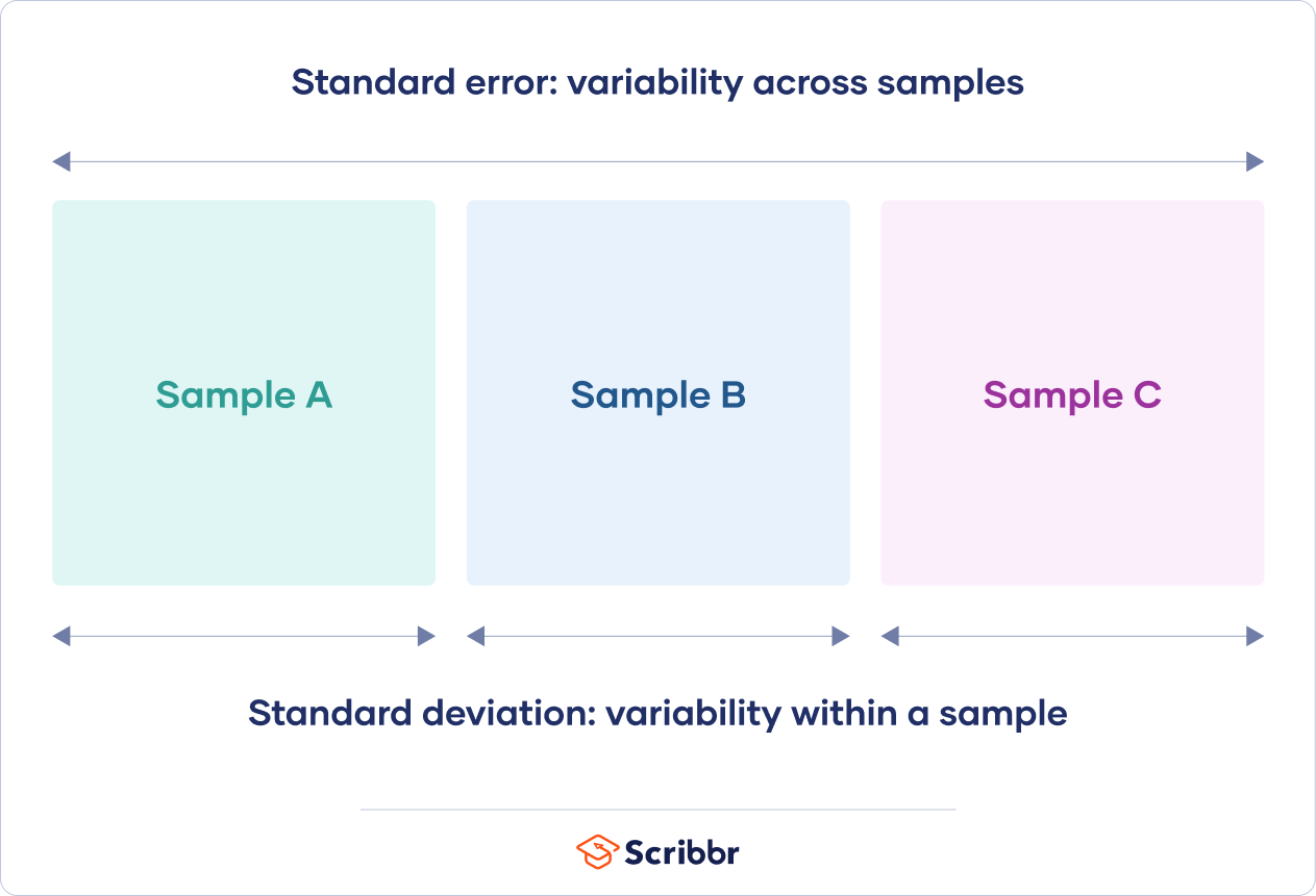
Standard error vs standard deviation

Standard error and standard deviation are both measures of variability:

The standard deviation describes variability within a single sample.
The standard error estimates the variability across multiple samples of a population.

The standard deviation is a descriptive statistic that can be calculated from sample data. In contrast, the standard error is an inferential statistic that can only be estimated (unless the real population parameter is known).

Example: Standard error vs standard deviation

In a random sample of 200 students, the mean math SAT score is 550. In this case, the sample is the 200 students, while the population is all test takers in the region.

The standard deviation of the math scores is 180. This number reflects on average how much each score differs from the sample mean score of 550.

The standard error of the math scores, on the other hand, tells you how much the sample mean score of 550 differs from other sample mean scores, in samples of equal size, in the population of all test takers in the region.

What can proofreading do for your paper?

Scribbr editors not only correct grammar and spelling mistakes, but also strengthen your writing by making sure your paper is free of vague language, redundant words, and awkward phrasing.

See editing example

Standard error formula

The standard error of the mean is calculated using the standard deviation and the sample size.

From the formula, you’ll see that the sample size is inversely proportional to the standard error. This means that the larger the sample, the smaller the standard error, because the sample statistic will be closer to approaching the population parameter.

Different formulas are used depending on whether the population standard deviation is known. These formulas work for samples with more than 20 elements (n > 20).

When population parameters are known

When the population standard deviation is known, you can use it in the below formula to calculate standard error precisely.

Formula	Explanation
$SE = dfrac{sigma}{sqrt{n}}$	is standard error is population standard deviation is the number of elements in the sample

When population parameters are unknown

When the population standard deviation is unknown, you can use the below formula to only estimate standard error. This formula takes the sample standard deviation as a point estimate for the population standard deviation.

Formula	Explanation
$SE = dfrac{s}{sqrt{n}}$	is standard error is sample standard deviation is the number of elements in the sample

Example: Using the standard error formula

To estimate the standard error for math SAT scores, you follow two steps.

First, find the square root of your sample size (n).

Formula

Calculation

Next, divide the sample standard deviation by the number you found in step one.

Formula	Calculation
$SE = dfrac{s}{sqrt{n}}$	$dfrac{s}{sqrt{n}} = dfrac{180}{14.1} = 12.8$

Formula

Calculation

$SE = dfrac{s}{sqrt{n}}$

$dfrac{s}{sqrt{n}} = dfrac{180}{14.1} = 12.8$

The standard error of math SAT scores is 12.8.

How should you report the standard error?

You can report the standard error alongside the mean or in a confidence interval to communicate the uncertainty around the mean.

Example: Reporting the mean and standard error

The mean math SAT score of a random sample of test takers is 550 ± 12.8 (SE).

The best way to report the standard error is in a confidence interval because readers won’t have to do any additional math to come up with a meaningful interval.

A confidence interval is a range of values where an unknown population parameter is expected to lie most of the time, if you were to repeat your study with new random samples.

With a 95% confidence level, 95% of all sample means will be expected to lie within a confidence interval of ± 1.96 standard errors of the sample mean.

Based on random sampling, the true population parameter is also estimated to lie within this range with 95% confidence.

Example: Constructing a 95% confidence interval

You construct a 95% confidence interval (CI) to estimate the population mean math SAT score.

For a normally distributed characteristic, like SAT scores, 95% of all sample means fall within roughly 4 standard errors of the sample mean.

Confidence interval formula
CI = x̄ ± (1.96 × SE) x̄ = sample mean = 550 SE = standard error = 12.8
Lower limit	Upper limit
x̄ − (1.96 × SE) 550 − (1.96 × 12.8) = 525	x̄ + (1.96 × SE) 550 + (1.96 × 12.8) = 575

Confidence interval formula

CI = x̄ ± (1.96 × SE)

x̄ = sample mean = 550
SE = standard error = 12.8

Lower limit

Upper limit

x̄ − (1.96 × SE)

550 − (1.96 × 12.8) = 525

x̄ + (1.96 × SE)

550 + (1.96 × 12.8) = 575

With random sampling, a 95% CI [525 575] tells you that there is a 0.95 probability that the population mean math SAT score is between 525 and 575.

Other standard errors

Aside from the standard error of the mean (and other statistics), there are two other standard errors you might come across: the standard error of the estimate and the standard error of measurement.

The standard error of the estimate is related to regression analysis. This reflects the variability around the estimated regression line and the accuracy of the regression model. Using the standard error of the estimate, you can construct a confidence interval for the true regression coefficient.

The standard error of measurement is about the reliability of a measure. It indicates how variable the measurement error of a test is, and it’s often reported in standardized testing. The standard error of measurement can be used to create a confidence interval for the true score of an element or an individual.

Frequently asked questions about standard error

What is standard error?: The standard error of the mean, or simply standard error, indicates how different the population mean is likely to be from a sample mean. It tells you how much the sample mean would vary if you were to repeat a study using new samples from within a single population.

Cite this Scribbr article

If you want to cite this source, you can copy and paste the citation or click the “Cite this Scribbr article” button to automatically add the citation to our free Citation Generator.

Bhandari, P.
(2022, December 19). What Is Standard Error? | How to Calculate (Guide with Examples). Scribbr.
Retrieved February 9, 2023,
from https://www.scribbr.com/statistics/standard-error/

Is this article helpful?

You have already voted. Thanks
Your vote is saved
Processing your vote…

Источник

Standard error of the sample mean[edit]

Exact value[edit]

Estimate[edit]

Accuracy of the estimator[edit]

Derivation[edit]

Independent and identically distributed random variables with random sample size[edit]

Student approximation when σ value is unknown[edit]

Assumptions and usage[edit]

Standard error of mean versus standard deviation[edit]

Extensions[edit]

Finite population correction (FPC)[edit]

Correction for correlation in the sample[edit]

See also[edit]

References[edit]

Example: Standard Error of the Estimate in Excel

Additional Resources

Video

References

About This Article

Did this article help you?

Why I Like the Standard Error of the Regression (S)

Стандартная ошибка по сравнению с R-квадратом в регрессии

Преимущества использования стандартной ошибки

Table of contents

Why standard error matters

Standard error vs standard deviation

What can proofreading do for your paper?

Standard error formula

When population parameters are known

When population parameters are unknown

How should you report the standard error?

Other standard errors

Frequently asked questions about standard error

Cite this Scribbr article

Is this article helpful?