Relative standard error

In statistics, a relative standard error (RSE) is equal to the standard error of a survey estimate divided by the survey estimate and then multiplied by 100. The number is multiplied by 100 so it can be expressed as a percentage. The RSE does not necessarily represent any new information beyond the standard error, but it might be a superior method of presenting statistical confidence.

Relative Standard Error vs. Standard Error

Standard error measures how much a survey estimate is likely to deviate from the actual population. It is expressed as a number. By contrast, relative standard error (RSE) is the standard error expressed as a fraction of the estimate and is usually displayed as a percentage. Estimates with an RSE of 25% or greater are subject to high sampling error and should be used with caution.

Survey Estimate and Standard Error

Surveys and standard errors are crucial parts of probability theory and statistics. Statisticians use standard errors to construct confidence intervals from their surveyed data. The reliability of these estimates can also be assessed in terms of a confidence interval. Confidence intervals are important for determining the validity of empirical tests and research.

A confidence interval is a type of interval estimate, computed from the statistics of the observed data, that might contain the true value of an unknown population parameter. Confidence intervals represent the range in which the population value is likely to lie. They are constructed using the estimate of the population value and its associated standard error. For example, there is approximately a 95% chance (i.e. 19 chances in 20) that the population value lies within two standard errors of the estimates, so the 95% confidence interval is equal to the estimate plus or minus two standard errors.

In layman’s terms, the standard error of a data sample is a measurement of the likely difference between the sample and the entire population. For example, a study involving 10,000 cigarette-smoking adults may generate slightly different statistical results than if every possible cigarette-smoking adult was surveyed.

Smaller sample errors are indicative of more reliable results. The central limit theorem in inferential statistics suggests that large samples tend to have approximately normal distributions and low sample errors.

Standard Deviation and Standard Error

The standard deviation of a data set is used to express the concentration of survey results. Less variety in the data results in a lower standard deviation. More variety is likely to result in a higher standard deviation.

The standard error is sometimes confused with the standard deviation. The standard error actually refers to the standard deviation of the mean. Standard deviation refers to the variability inside any given sample, while a standard error is the variability of the sampling distribution itself.

The standard error is an absolute gauge between the sample survey and the total population. The relative standard error shows if the standard error is large relative to the results; large relative standard errors suggest the results are not significant. The formula for relative standard error is:

Relative Standard Error

Standard Error

Estimate

where:

Standard Error

standard deviation of the mean sample

Estimate

mean of the sample

begin{aligned} &text{Relative Standard Error} = frac { text{Standard Error} }{ text{Estimate} } times 100 \ &textbf{where:} \ &text{Standard Error} = text{standard deviation of the mean sample} \ &text{Estimate} = text{mean of the sample} \ end{aligned}

Relative Standard Error=EstimateStandard Error×100where:Standard Error=standard deviation of the mean sampleEstimate=mean of the sample

Источник

From Simple English Wikipedia, the free encyclopedia

For a value that is sampled with an unbiased normally distributed error, the above depicts the proportion of samples that would fall between 0, 1, 2, and 3 standard deviations above and below the actual value.

The standard error, sometimes abbreviated as ,^[1] is the standard deviation of the sampling distribution of a statistic.^[2] The term may also be used for an estimate (good guess) of that standard deviation taken from a sample of the whole group.

The average of some part of a group (called a sample) is the usual way to estimate the average for the whole group. It is often too hard or too costly to measure the whole group. But if a different sample is measured, it will have an average that is a little bit different from the first sample. The standard error of the mean is a way to know how close the average of the sample is to the average of the whole group. It is a way of knowing how sure one can be about the average from the sample.

In real measurements, the true value of the standard deviation of the mean for the whole group is usually not known. So the term standard error is often used to mean a close guess to the true number for the whole group. The more measurements there are in a sample, the closer the guess will be to the true number for the whole group.

How to find standard error of the mean[change | change source]

One way to find the standard error of the mean is to have lots of samples. First, the average for each sample is found. Then the average and standard deviation of those sample averages is found. The standard deviation for all the sample averages is the standard error of the mean. This can be a lot of work. Sometimes it is too difficult or costly to have lots of samples.

Another way to find the standard error of the mean is to use an equation that needs only one sample. Standard error of the mean is usually estimated by the standard deviation for a sample from the whole group (sample standard deviation), divided by the square root of the sample size:^[3]

${displaystyle SE_{bar {x}} ={frac {s}{sqrt {n}}}}$

where

s is the sample standard deviation (i.e., the sample-based estimate of the standard deviation of the population), and

n is the number of measurements in the sample.

In general, the larger the sample, the closer the estimated standard error of the mean is to the actual standard error of the mean. As a rule of thumb, there should be at least six measurements in a sample. Then the standard error of the mean for the sample will be within 5% of the actual standard error of the mean (that is, if the whole group were measured).^[4]

Corrections for some cases[change | change source]

There is another equation to use if the number of measurements is for 5% or more of the whole group:^[5]

There are special equations to use if a sample has less than 20 measurements.^[6]

Sometimes, a sample may come from one place even though the whole group may be spread out, while other times, a sample may be made in a short time period when the whole group covers a longer time. In which case, the numbers in the sample are not independent, and special equations are used to try to correct for this.^[7]

Usefulness[change | change source]

A practical result: One can become more sure of an average value by having more measurements in a sample. Then the standard error of the mean will be smaller because the standard deviation is divided by a bigger number. However, to make the uncertainty (standard error of the mean) in an average value half as big, the sample size (n) needs to be four times bigger. This is because the standard deviation is divided by the square root of the sample size. To make the uncertainty one-tenth as big, the sample size (n) needs to be one hundred times bigger.

Standard errors are easy to calculate and commonly used because:

If the standard error of several individual quantities is known, then the standard error of some function of the quantities can be easily calculated in many cases;
Where the probability distribution of the value is known, it can be used to calculate a good approximation to an exact confidence interval;
Where the probability distribution is not known, other equations can be used to estimate a confidence interval;
As the sample size gets very large, the principle of the central limit theorem shows that the numbers in the sample are very much like the numbers in the whole group (they follow a normal distribution).

Relative standard error[change | change source]

The relative standard error (RSE) is the standard error divided by the average. This number is smaller than one. Multiplying it by 100% gives it as a percentage of the average. This helps to show whether the uncertainty is important or not.

For example, consider two surveys of household income that both result in a sample average of $50,000. If one survey has a standard error of $10,000 and the other has a standard error of $5,000, then the relative standard errors are 20% and 10%, respectively. The survey with the lower relative standard error is better, because it has a more precise measurement (the uncertainty is smaller).

In fact, people who need to know average values often decide how small the uncertainty should be—before they decide to use the information. For example, the U.S. National Center for Health Statistics does not report an average if the relative standard error exceeds 30%. NCHS also requires at least 30 observations for an estimate to be reported.^[source?]

Example[change | change source]

Example of a redfish (also known as red drum, Sciaenops ocellatus) used in the example.

For example, there are many redfish in the water of the Gulf of Mexico. To find out how much a 42 cm long redfish weighs on average, it is not possible to measure all of the redfish that are 42 cm long. Instead, it is possible to measure some of them. The fish that are actually measured are called a sample. The table shows weights for two samples of redfish, all 42 cm long. The average (mean) weight of the first sample is 0.741 kg. The average (mean) weight of the second sample is 0.735 kg—a little bit different from the first sample. Each of these averages is a little bit different from the average that would come from measuring every 42 cm long redfish (which is not possible anyway).

The uncertainty in the mean can be used to know how close the average of the samples are to the average that would come from measuring the whole group. The uncertainty in the mean is estimated as the standard deviation for the sample, divided by the square root of the number of samples minus one. The table shows that the uncertainties in the means for the two samples are very close to each other. Also, the relative uncertainty is the uncertainty in the mean divided by the mean, times 100%. The relative uncertainty in this example is 2.38% and 2.50% for the two samples.

Knowing the uncertainty in the mean, one can know how close the sample average is to the average that would come from measuring the whole group. The average for the whole group is between a) the average for the sample plus the uncertainty in the mean, and b) the average for the sample minus the uncertainty in the mean. In this example, the average weight for all of the 42 cm long redfish in the Gulf of Mexico is expected to be 0.723–0.759 kg based on the first sample, and 0.717–0.753 based on the second sample.

[change | change source]

Errors and residuals in statistics

References[change | change source]

↑ «List of Probability and Statistics Symbols». Math Vault. 2020-04-26. Retrieved 2020-09-12.
↑ Everitt B.S. 2003. The Cambridge Dictionary of Statistics, CUP. ISBN 0-521-81099-X
↑ Altman, Douglas G; Bland, J Martin (2005-10-15). «Standard deviations and standard errors». BMJ : British Medical Journal. 331 (7521): 903. doi:10.1136/bmj.331.7521.903. ISSN 0959-8138. PMC 1255808. PMID 16223828.
↑ Gurland, John; Tripathi, Ram C. (1971). «A simple approximation for unbiased estimation of the standard deviation». American Statistician. American Statistical Association. 25 (4): 30–32. doi:10.2307/2682923. JSTOR 2682923.
↑ Isserlis, L. (1918). «On the value of a mean as calculated from a sample». Journal of the Royal Statistical Society. Blackwell Publishing. 81 (1): 75–81. doi:10.2307/2340569. JSTOR 2340569. (Equation 1)
↑ Sokal and Rohlf 1981. Biometry: principles and practice of statistics in biological research, 2nd ed. p53 ISBN 0716712547
↑ James R. Bence 1995. Analysis of short time series: correcting for autocorrelation. Ecology 76(2): 628–639.

Источник

Explaining measures of uncertainty such as standard error, confidence interval, coefficient of variation and statistical significance and how they affect estimates from our surveys.

1. What is uncertainty?

Many of our statistics rely on data collected from surveys. We are often interested in the characteristics of the population of people or businesses as a whole, but usually survey a sample of the population rather than everyone. This is timelier and more cost-effective and, if the sample is large enough and well designed, can lead to accurate statistics.

Using a sample means that our statistics are usually accompanied by measures of uncertainty. Uncertainty relates to how the estimate might differ from the “true value” and these measures help users of ONS statistics to understand the degree of confidence in the outputs. These measures of uncertainty include:

standard error
confidence interval
coefficient of variation
statistical significance

Understanding sampling and the effect it has on statistics is also important for interpreting these measures of uncertainty.

Back to table of contents

2. Sampling the population

Sampling involves selecting a subset of a population from which characteristics of the entire population can be estimated. Surveying a sample rather than an entire population is more-cost effective and allows data and findings to be published sooner.

Information is not gathered from the whole population, so results from sample surveys are estimates of the unknown population values. One sample is selected at random but other potential samples could have been selected, which may have produced different results.

The difference between a statistic derived from a sample and the population value is caused by what are known as sampling error and non-sampling errors.

Sampling error

Sampling error is caused by the use of a sample of the population, rather than the entire population. Estimates derived from a sample are likely to differ from the unknown population value because only a subset of the population have provided information. Designing a sample using a scientific approach can help to minimise sampling error and create estimates that are precise and unbiased.

The standard error, coefficient of variation and confidence interval can be used to help interpret the possible sampling error, which of course, is unknown. Standard errors are important for interpreting changes in the population estimates over time. A test of statistical significance could be used to decide whether the difference between estimates from different samples is caused by a real change in the population, or whether it is because of the effects of random sampling alone.

Non-sampling errors

Other sources of error are called non-sampling errors. These include:

businesses or individuals being unreachable
businesses or individuals refusing to respond
respondents giving inaccurate answers
processing or analysis errors

These errors would be present in the statistics even if the entire population had been surveyed. For example, inaccurate answers to a question about money spent on fuel would lead to a difference between the estimate and the population value even if the entire population were surveyed. These errors are usually very difficult to quantify and to do so would require additional and specific research.

Back to table of contents

3. Standard error

The standard error is the simplest measure of how precise a survey-based estimate is.

The standard error can be used as a guide to help interpret the possible sampling error. It shows how close the estimate based on sample data might be to the value that would have been taken from the whole population. It is measured using the same units as the estimate itself and, in general, the closer the standard error is to zero, the more precise the estimate. Smaller values show a greater level of precision.

Standard errors are also based on sample data so are an unknown statistic, and are usually estimated themselves.

Example:

The non-financial business economy estimates are taken from the Annual Business Survey. The standard error for estimates of various industry sectors is used to assess how precise total turnover estimates are. The estimates for education, and water and waste management differ in size, as do their standard errors. However, the relative standard errors show they have similar levels of relative precision (Table 1).

Download this table Table 1: Total turnover estimates, standard error and relative standard error for education and water and waste management, UK, 2016

.xls
.csv

Notes:

Data are from Non-financial business economy, UK: Sections A to A 2017 revised results.
Data are from Non-financial business economy, UK: quality measures 2017 revised results.

Back to table of contents

4. Coefficient of variation

The coefficient of variation makes it easier to understand whether a standard error is large compared with the estimate itself.

The coefficient of variation (CV) is used to compare the relative precision across surveys (or variables) and is usually shown as a percentage. It is a unitless quantity, and so allows us to compare estimates with different scales of measurement. It is also known as the relative standard error and is calculated by dividing the standard error of an estimate by the estimate itself.

Similar to the standard error, the closer the coefficient of variation is to zero, the more precise the estimate is. Where it is above 50%, the estimate is very unprecise and the confidence intervals around the estimate will effectively contain zero.

The coefficient of variation should not be used for estimates of values that are close to zero or for percentages.

Example:

The total turnover of plastering businesses in the UK was estimated at £2,322 million in 2016, with a standard error of £201 million. A different survey estimated that the total number of people employed full-time in agriculture, forestry and fishing in the UK was 155,000 in 2016, with a standard error of 12,400 employees

It is difficult to compare these two standard errors. By calculating the coefficient of variation for each, the results show that both estimates have a similar level of precision:

£201 million divided by £2,322 million equals 0.087 – a coefficient of variation of 8.7%
12,400 divided by 155,000 equals 0.08 – a coefficient of variation of 8%

The data for this example are from Non-financial business economy, UK: Sections A to S, Non-financial business economy, UK: quality measures, and Broad Industry Group (SIC) – Business Register and Employment Survey (BRED): Table 1.

Back to table of contents

5. Confidence interval

Confidence intervals use the standard error to derive a range in which we think the true value is likely to lie.

A confidence interval gives an indication of the degree of uncertainty of an estimate and helps to decide how precise a sample estimate is. It specifies a range of values likely to contain the unknown population value. These values are defined by lower and upper limits.

The width of the interval depends on the precision of the estimate and the confidence level used. A greater standard error will result in a wider interval; the wider the interval, the less precise the estimate is.

Using a 95% confidence interval

A 95% confidence level is frequently used. This means that if we drew 20 random samples and calculated a 95% confidence interval for each sample using the data in that sample, we would expect that, on average, 19 out of the 20 (95%) resulting confidence intervals would contain the true population value and 1 in 20 (5%) would not. If we increased the confidence level to 99%, wider intervals would be obtained.

Example:

Estimates for July to September 2019 show 32.75 million people aged 16 years and over in employment in the UK, with a confidence interval of plus or minus 177,000 people based on the results from a sample. If we took a large number of samples repeatedly, 95% of the confidence intervals would contain the unknown population estimate.

The data for this example are from Labour market overview, UK: November 2019 and A11: Labour Force Survey sampling variability.

Calculating confidence intervals

To calculate confidence intervals around an estimate we use the standard error for that estimate. The estimate and its 95% confidence interval are presented as: the estimate plus or minus the margin of error.

The lower and upper 95% confidence limits are given by the sample estimate plus or minus 1.96 standard errors.

The margin of error is calculated as:

Margin of error = 1.96 × standard error

Example:

In 2016, the UK private education industry was estimated to have generated a total turnover of £42,649 million. The standard error for this estimate is £526.8 million.

The 95% confidence interval around this estimate is calculated as:

Margin of error = 1.96 × £526.8 million = £1,032.5 million

The 95% confidence interval is therefore £42,649 million plus or minus £1,032.5 million, which equals £41,616 million and £43,682 million respectively.

This means that if we drew 20 random samples and calculated an analogous confidence interval for each, on average, 19 out of 20 (95%) would contain the true population value and 1 in 20 (5%) would not. Therefore, there is a 95% chance that the true population value lies between £41,616 million and £43,682 million.

Data for this example come from Non-financial business economy, UK: Sections A to S 2017 revised results and Non-financial business economy, UK: quality measures 2017 revised results.

Back to table of contents

6. Statistical significance

We can use statistical significance to decide whether we think a difference between two survey-based estimates reflects a true change in the population rather than being attributable to random variation in our sample selection.

Statistical significance helps us to establish what observed changes or relationships we should pay attention to, and which apparent changes may have occurred only as a result of randomness in the sampling.

A result is said to be statistically significant if it is likely not caused by chance or the variable nature of the samples. A defined threshold can help us test for change. If the test of statistical significance calculated from the estimates at different points in time is larger than the threshold, the change is said to be “statistically significant”.

A 5% standard is often used when testing for statistical significance. The observed change is statistically significant at the 5% level if there is less than a 1 in 20 chance of the observed change being calculated by chance if there is actually no underlying change.

Within the commentary of our statistical bulletins we will avoid using the term “significant” to describe trends in our statistics and will always use “statistically significant” to avoid any confusion for our users.

Example:

Estimates from the Annual Population Survey are based upon one of several samples that could have been drawn at that point in time. This means there is a degree of variability around the estimates. This can sometimes present misleading changes in figures because the people included in the sample are selected at random.

Figure 1: There has been a statistically significant decrease in the prevalence of smoking in the UK in 2018 compared with 2011

Proportion who were current smokers, all persons aged 18 years and over, UK, 2011 to 2018

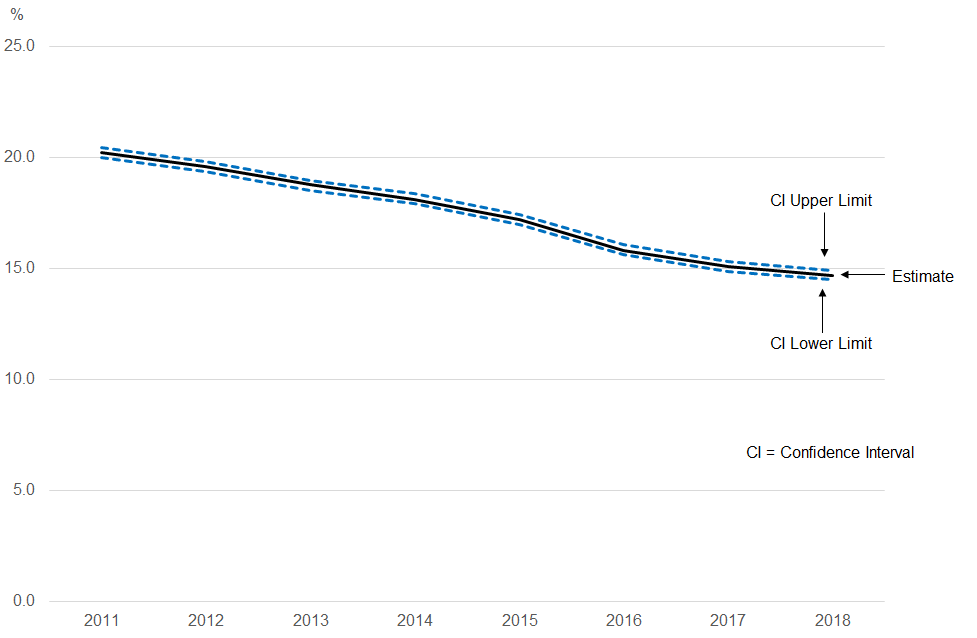
Source: Office for National Statistics – Annual Population Survey

Download this image Figure 1: There has been a statistically significant decrease in the prevalence of smoking in the UK in 2018 compared with 2011

.png (15.8 kB)
.xlsx (160.9 kB)

The proportion of people aged 18 years and over smoking cigarettes in the UK is estimated to have changed from 20.2% in 2011 to 14.7% in 2018. But we cannot assume that this change represents a real decrease in the prevalence of smoking. It could be the result of variations in the sample estimates, which make the differences between the estimates larger than the real change in smoking prevalence.

The test of statistical significance found that the difference between the estimates was larger than expected if it had only been caused by random sampling. This means that the difference is likely to reflect a true decrease in the prevalence of smoking in the UK between 2011 and 2018 rather than being attributable to random variation in our sample selection between these two years.

Back to table of contents

7. Related links

Quality defined
Article
A summary of the work ONS is doing to monitor and improve the quality of our outputs and statistics.

Types of official statistics
Article
Summarises the main types of official statistics produced by public bodies, including National Statistics and Experimental Statistics.

Code of Practice for Statistics
Report | February 2018
Provides producers of official statistics with the detailed practices they must commit to.

Back to table of contents

Источник

Для значения, которое выбирается с несмещенной ошибкой с нормальным распределением , приведенное выше показывает долю выборок, которая будет находиться между 0, 1, 2 и 3 стандартными отклонениями выше и ниже фактического значения.

Стандартная ошибка ( SE ) ^[1]^[2] из статистики (обычно подсчет параметра ) является стандартным отклонением ее выборочным распределения ^[3] или оценка этого стандартного отклонения. Если статистика является выборочным средним, это называется стандартной ошибкой среднего ( SEM ). ^[2]

Распределение выборки из среднего генерируется путем повторного отбора образцов из того же населения и записи средств , полученных образцов. Это формирует распределение различных средних, и это распределение имеет собственное среднее значение и дисперсию . Математически дисперсия полученного распределения выборки равна дисперсии генеральной совокупности, деленной на размер выборки. Это связано с тем, что по мере увеличения размера выборки средние значения выборки сгруппируются более близко к среднему значению генеральной совокупности.

Следовательно, соотношение между стандартной ошибкой среднего и стандартным отклонением таково, что для данного размера выборки стандартная ошибка среднего равна стандартному отклонению, деленному на квадратный корень из размера выборки. ^[2] Другими словами, стандартная ошибка среднего — это мера разброса средних значений выборки вокруг среднего значения генеральной совокупности.

В регрессионном анализе термин «стандартная ошибка» относится либо к квадратному корню из приведенной статистики хи-квадрат , либо к стандартной ошибке для конкретного коэффициента регрессии (который используется, например, в доверительных интервалах ).

Стандартная ошибка среднего

Точное значение

Если статистически независимая выборка наблюдения берутся из статистической совокупности с стандартным отклонением от, то среднее значение, рассчитанное по выборке будет связана стандартная ошибка среднего предоставлено: ^[2]

На практике это говорит нам о том, что при попытке оценить значение среднего по совокупности из-за фактора для уменьшения ошибки оценки в два раза требуется получить в четыре раза больше наблюдений в выборке; уменьшение его в десять раз требует в сто раз больше наблюдений.

Оценить

Стандартное отклонение о выборке населения известно редко. Поэтому стандартная ошибка среднего обычно оценивается заменойсо стандартным отклонением выборки вместо:

Поскольку это только оценка истинной «стандартной ошибки», здесь часто встречаются другие обозначения, такие как:

или поочередно .

Обычный источник путаницы возникает, когда не удается четко различить стандартное отклонение совокупности (), стандартное отклонение выборки (), стандартное отклонение самого среднего (, которая является стандартной ошибкой), и оценка стандартного отклонения среднего (, которая является наиболее часто вычисляемой величиной, которую также часто называют стандартной ошибкой ).

Точность оценщика

Когда размер выборки невелик, использование стандартного отклонения выборки вместо истинного стандартного отклонения генеральной совокупности будет иметь тенденцию к систематическому занижению стандартного отклонения генеральной совокупности, а, следовательно, и стандартной ошибки. При n = 2 занижение составляет около 25%, но для n = 6 занижение составляет всего 5%. Гурланд и Трипати (1971) предлагают поправку и уравнение для этого эффекта. ^[4] Сокал и Рольф (1981) приводят уравнение поправочного коэффициента для малых выборок n <20. ^[5] См. Несмещенную оценку стандартного отклонения для дальнейшего обсуждения.

Вывод

Стандартная ошибка среднего может быть получена из дисперсии суммы независимых случайных величин ^{[6] с} учетом определения дисперсии и некоторых ее простых свойств . Если находятся независимые наблюдения от популяции со средним и стандартное отклонение , то мы можем определить общую

которые по формуле Биенайме будут иметь дисперсию

Среднее значение этих измерений просто дается

Тогда дисперсия среднего составляет

Стандартная ошибка — это, по определению, стандартное отклонение который представляет собой просто квадратный корень из дисперсии:

Для коррелированных случайных величин дисперсия выборки должна быть вычислена в соответствии с центральной предельной теоремой Маркова .

Независимые и одинаково распределенные случайные величины со случайным размером выборки

Бывают случаи, когда образец берут, не зная заранее, сколько наблюдений будет приемлемым по какому-либо критерию. В таких случаях размер выборки случайная величина, вариация которой добавляет к вариации такой, что,

^[7]

Если имеет распределение Пуассона , то с оценщиком . Следовательно, оценка становится , приводя к следующей формуле для стандартной ошибки:

(поскольку стандартное отклонение — это квадратный корень из дисперсии)

Аппроксимация Стьюдента, когда значение σ неизвестно

Во многих практических приложениях истинное значение σ неизвестно. В результате нам нужно использовать распределение, которое учитывает этот разброс возможных σ ‘с. Когда известно, что истинное базовое распределение является гауссовым, хотя и с неизвестным σ, тогда полученное оцененное распределение следует t-распределению Стьюдента. Стандартная ошибка — это стандартное отклонение t-распределения Стьюдента. Т-распределения немного отличаются от гауссовых и меняются в зависимости от размера выборки. Небольшие выборки с большей вероятностью недооценивают стандартное отклонение совокупности и имеют среднее значение, которое отличается от истинного среднего значения совокупности, а t-распределение Стьюдента учитывает вероятность этих событий с несколько более тяжелыми хвостами по сравнению с гауссовым. Для оценки стандартной ошибки t-распределения Стьюдента достаточно использовать выборочное стандартное отклонение «s» вместо σ , и мы могли бы использовать это значение для вычисления доверительных интервалов.

Примечание. Распределение вероятностей Стьюдента хорошо аппроксимируется распределением Гаусса, когда размер выборки превышает 100. Для таких выборок можно использовать последнее распределение, которое намного проще.

Предположения и использование

Пример того, как используется, чтобы сделать доверительные интервалы неизвестного среднего значения в генеральной совокупности. Если распределение выборки имеет нормальное распределение , среднее значение выборки, стандартная ошибка и квантили нормального распределения могут использоваться для расчета доверительных интервалов для истинного среднего значения генеральной совокупности. Следующие выражения можно использовать для расчета верхнего и нижнего 95% доверительных интервалов, где равно выборочному среднему, равна стандартной погрешности для выборочного среднего и 1,96 приблизительное значение 97,5 процентиля точки нормального распределения :

Верхний предел 95% а также

Нижний предел 95%

В частности, стандартная ошибка выборочной статистики (например, выборочное среднее ) — это фактическое или расчетное стандартное отклонение выборочного среднего в процессе, в котором оно было создано. Другими словами, это фактическое или оценочное стандартное отклонение выборочного распределения статистической выборки. Обозначение для стандартной ошибки может быть любым из SE, SEM (для стандартной ошибки измерения или среднего ), или S _E .

Стандартные ошибки обеспечивают простые меры неопределенности значения и часто используются, потому что:

во многих случаях, если известна стандартная ошибка нескольких отдельных величин, то стандартную ошибку некоторой функции величин можно легко вычислить;
когда распределение вероятностей значения известно, его можно использовать для вычисления точного доверительного интервала ;
когда распределение вероятностей неизвестно, для расчета консервативного доверительного интервала можно использовать неравенства Чебышева или Высочанского – Петунина ; а также
поскольку размер выборки стремится к бесконечности, центральная предельная теорема гарантирует, что выборочное распределение среднего является асимптотически нормальным .

Стандартная ошибка среднего значения по сравнению со стандартным отклонением

В научно-технической литературе экспериментальные данные часто обобщаются либо с использованием среднего значения и стандартного отклонения выборочных данных, либо среднего значения со стандартной ошибкой. Это часто приводит к путанице в отношении их взаимозаменяемости. Однако среднее значение и стандартное отклонение являются описательной статистикой , тогда как стандартная ошибка среднего описывает процесс случайной выборки. Стандартное отклонение данных выборки — это описание вариации в измерениях, в то время как стандартная ошибка среднего — это вероятностное утверждение о том, как размер выборки обеспечит лучшую границу оценок среднего для генеральной совокупности в свете центрального предела. теорема. ^[8]

Проще говоря, стандартная ошибка выборочного среднего — это оценка того, насколько далеко среднее значение выборки может быть от среднего значения по совокупности, тогда как стандартное отклонение выборки — это степень, в которой отдельные лица в выборке отличаются от выборочного среднего. ^[9] Если стандартное отклонение генеральной совокупности конечно, стандартная ошибка среднего значения выборки будет стремиться к нулю с увеличением размера выборки, потому что оценка генерального среднего будет улучшаться, в то время как стандартное отклонение выборки будет иметь тенденцию приближаться стандартное отклонение генеральной совокупности при увеличении размера выборки.

Расширения

Поправка на конечную популяцию (FPC)

Приведенная выше формула для стандартной ошибки предполагает, что размер выборки намного меньше, чем размер генеральной совокупности, так что совокупность может считаться фактически бесконечной по размеру. Обычно это имеет место даже в случае конечных популяций, потому что большую часть времени люди в первую очередь заинтересованы в управлении процессами, которые создали существующую конечную популяцию; это называется аналитическим исследованием вслед за У. Эдвардсом Демингом . Если люди заинтересованы в управлении существующей конечной совокупностью, которая не будет меняться с течением времени, то необходимо сделать поправку на размер популяции; это называется перечислительным исследованием .

Когда доля выборки (часто называемая f ) велика (примерно 5% или более) в переписном исследовании , оценка стандартной ошибки должна быть скорректирована путем умножения на «поправку на конечную совокупность» (также известную как fpc ): ^[10]
^[11]

что для больших N :

чтобы учесть дополнительную точность, полученную за счет выборки, близкой к большему проценту населения. Эффект FPC является то , что ошибка становится равной нулю , когда размер выборки п равен размеру популяции N .

Это происходит в методологии обследования при выборке без замены . Если выборка с заменой, то FPC не играет роли.

Поправка на корреляцию в образце

Ожидаемая ошибка среднего значения A для выборки из n точек данных с коэффициентом смещения выборки ρ . Несмещенная стандартная ошибка строится как диагональная линия ρ = 0 с логарифмическим наклоном −½.

Если значения измеренной величины A не являются статистически независимыми, но были получены из известных мест в пространстве параметров x , несмещенная оценка истинной стандартной ошибки среднего (фактически поправка на часть стандартного отклонения) может быть получена путем умножения рассчитанная стандартная ошибка выборки по коэффициенту f :

где коэффициент смещения выборки ρ представляет собой широко используемую оценку Прайса – Винстена коэффициента автокорреляции (величина от -1 до +1) для всех пар точек выборки. Эта приблизительная формула предназначена для выборки среднего и большого размера; Справочник дает точные формулы для любого размера выборки и может применяться к сильно автокоррелированным временным рядам, таким как котировки акций Уолл-стрит. Более того, эта формула работает как для положительных, так и для отрицательных значений ρ. ^[12] См. Также объективную оценку стандартного отклонения для более подробного обсуждения.

См. Также

Иллюстрация центральной предельной теоремы
Допустимая погрешность
Вероятная ошибка
Стандартная ошибка средневзвешенного значения
Среднее значение выборки и ковариация выборки
Стандартная ошибка медианы
Дисперсия

Ссылки

^ «Список вероятностных и статистических символов» . Математическое хранилище . 2020-04-26 . Проверено 12 сентября 2020 .
^ ^a ^b ^c ^d Альтман, Дуглас Дж. Блэнд, Дж. Мартин (2005-10-15). «Стандартные отклонения и стандартные ошибки» . BMJ: Британский медицинский журнал . 331 (7521): 903. DOI : 10.1136 / bmj.331.7521.903 . ISSN 0959-8138 . PMC 1255808 . PMID 16223828 .
^ Everitt, BS (2003). Кембриджский статистический словарь . ЧАШКА. ISBN 978-0-521-81099-9.
^ Gurland, J; Трипати RC (1971). «Простое приближение для объективной оценки стандартного отклонения». Американский статистик . 25 (4): 30–32. DOI : 10.2307 / 2682923 . JSTOR 2682923 .
^ Сокаль; Рольф (1981). Биометрия: принципы и практика статистики в биологических исследованиях (2-е изд.). п. 53 . ISBN 978-0-7167-1254-1.
Перейти ↑ Hutchinson, TP (1993). Основы статистических методов, на 41 странице . Аделаида: Рамсби. ISBN 978-0-646-12621-0.
^ Корнелл, младший, и Бенджамин, Калифорния, Вероятность, статистика и решения для инженеров-строителей, McGraw-Hill, NY, 1970, ISBN 0486796094 , стр. 178–9.
^ Бард, М. (2012). «Что использовать для выражения изменчивости данных: стандартное отклонение или стандартная ошибка среднего?» . Перспектива. Clin. Res. 3 (3): 113–116. DOI : 10.4103 / 2229-3485.100662 . PMC 3487226 . PMID 23125963 .
^ Wassertheil-Smoller, Sylvia (1995). Биостатистика и эпидемиология: учебник для медицинских работников (второе изд.). Нью-Йорк: Спрингер. С. 40–43. ISBN 0-387-94388-9.
^ Isserlis, Л. (1918). «О значении среднего, рассчитанного по выборке» . Журнал Королевского статистического общества . 81 (1): 75–81. DOI : 10.2307 / 2340569 . JSTOR 2340569 . (Уравнение 1)
^ Бонди, Уоррен; Злот, Уильям (1976). «Стандартная ошибка среднего и разница между средними для конечных совокупностей». Американский статистик . 30 (2): 96–97. DOI : 10.1080 / 00031305.1976.10479149 . JSTOR 2683803 . (Уравнение 2)
^ Бенс, Джеймс Р. (1995). «Анализ коротких временных рядов: поправка на автокорреляцию» . Экология . 76 (2): 628–639. DOI : 10.2307 / 1941218 . JSTOR 1941218 .

Источник

Purpose
Calculation of the standard errors
Running the standard errors task
Outputs
- In the graphical user interface
- In the output folder
Interpreting the correlation matrix of the estimates
Settings
Good practice

Purpose

The standard errors represent the uncertainty of the estimated population parameters. In Monolix, they are calculated via the estimation of the Fisher Information Matrix. They can for instance be used to calculate confidence intervals or detect model overparametrization.

Calculation of the standard errors

Several methods have been proposed to estimate the standard errors, such as bootstrapping or via the Fisher Information Matrix (FIM). In the Monolix GUI, the standard errors are estimated via the FIM. Bootstrapping is available via the Rsmlx R package.

The Fisher Information Matrix (FIM)

The observed Fisher information matrix (FIM) (I ) is minus the second derivatives of the observed log-likelihood:

$$ I(hat{theta}) = -frac{partial^2}{partialtheta^2}log({cal L}_y(hat{theta})) $$

The log-likelihood cannot be calculated in closed form and the same applies to the Fisher Information Matrix. Two different methods are available in Monolix for the calculation of the Fisher Information Matrix: by linearization or by stochastic approximation.

Via stochastic approximation

A stochastic approximation algorithm using a Markov chain Monte Carlo (MCMC) algorithm is implemented in Monolix for estimating the FIM. This method is extremely general
and can be used for many data and model types (continuous, categorical, time-to-event, mixtures, etc.).

Via linearization

This method can be applied for continuous data only. A continuous model can be written as:

$$begin{array}{cl} y_{ij} &= f(t_{ij},z_i)+g(t_{ij},z_i)epsilon_{ij} \ z_i &= z_{pop}+eta_i end{array}$$

with ( y_{ij} ) the observations, f the prediction, g the error model, ( z_i) the individual parameter value for individual i, ( z_{pop}) the typical parameter value within the population and (eta_i) the random effect.
Linearizing the model means using a Taylor expansion in order to approximate the observations ( y_{ij} ) by a normal distribution. In the formulation above, the appearance of the random variable (eta_i) in the prediction f in a nonlinear way leads to a complex (non-normal) distribution for the observations ( y_{ij} ).
The Taylor expansion is done around the EBEs value, that we note ( z_i^{textrm{mode}} ).

Standard errors

Once the Fisher Information Matrix has been obtained, the standard errors can be calculated as the square root of the diagonal elements of the inverse of the Fisher Information Matrix. The inverse of the FIM (I(hat{theta})) is the variance-covariance matrix (C(hat{theta})):

$$C(hat{theta})=I(hat{theta})^{-1}$$

The standard error for parameter ( hat{theta}_k ) can be calculated as:

$$textrm{s.e}(hat{theta}_k)=sqrt{tilde{C}_{kk}(hat{theta})}$$

Note that in Monolix, the Fisher Information Matrix and variance-covariance matrix are calculated on the transformed normally distributed parameters. The variance-covariance matrix ( tilde{C} ) for the untransformed parameters can be obtained using the jacobian (J):

$$tilde{C}=J^TC J$$

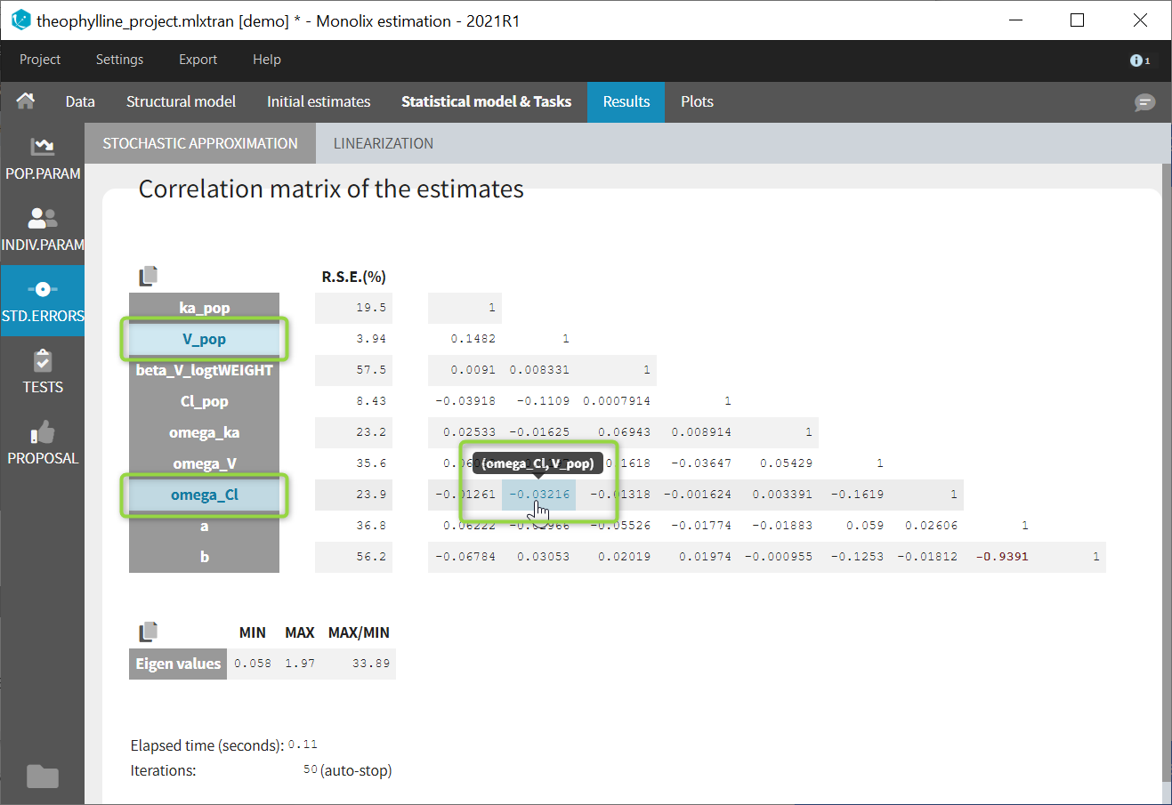
Correlation matrix

The correlation matrix is calculated from the variance-covariance matrix as:

$$text{corr}(theta_i,theta_j)=frac{tilde{C}_{ij}}{textrm{s.e}(theta_i)textrm{ s.e}(theta_j)}$$

Wald test

For the beta parameters characterizing the influence of the covariates, the relative standard error can be used to perform a Wald test, testing if the estimated beta value is significantly different from zero.

Running the standard errors task

When running the standard error task, the progress is displayed in the pop-up window. At the end of the task, the correlation matrix is also shown, along with the elapsed time and number of iterations.

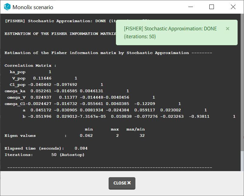
Dependencies between tasks:

The “Population parameters” task must be run before launching the Standard errors task. If the Conditional distribution task has already been run, the first iterations of the Standard errors (without linearization) will be very fast, as they will reuse the same draws as those obtained in the Conditional distribution task.

Output

In the graphical user interface

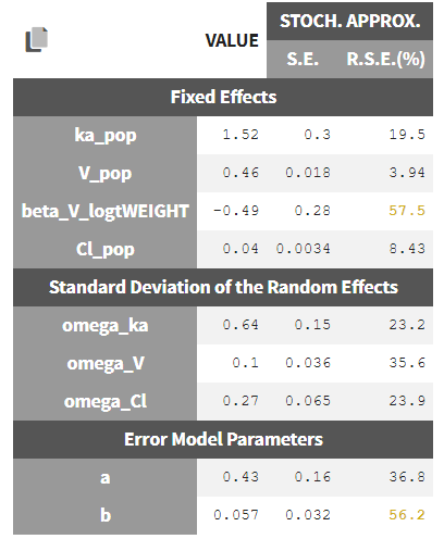
In the Pop.Param section of the Results tab, three additional columns appear in addition to the estimated population parameters:

S.E: the estimated standard errors
R.S.E: the relative standard error (standard error divided by the estimated parameter value)

To help the user in the interpretation, a color code is used for the p-value and the RSE:

For the p-value: between .01 and .05, between .001 and .01, and less than .001.
For the RSE: between 50% and 100%, between 100% and 200%, and more than 200%.

When the standard errors were estimated both with and without linearization, the S.E and R.S.E are displayed for both methods.

In the STD.ERRORS section of the Results tab, we display:

R.S.E: the relative standard errors
Correlation matrix: the correlation matrix of the population parameters
Eigen values: the smallest and largest eigen values, as well as the condition number (max/min)
The elapsed time and, starting from Monolix2021R1, the number of iterations for stochastic approximation, as well as a message indicating whether convergence has been reached (“auto-stop”) or if the task was stopped by the user or reached the maximum number of iterations.

To help the user in the interpretation, a color code is used:

For the correlation: between .5 and .8, between .8 and .9, and higher than .9.
For the RSE: between 50% and 100%, between 100% and 200%, and more than 200%.

When the standard errors were estimated both with and without linearization, both results appear in different subtabs.

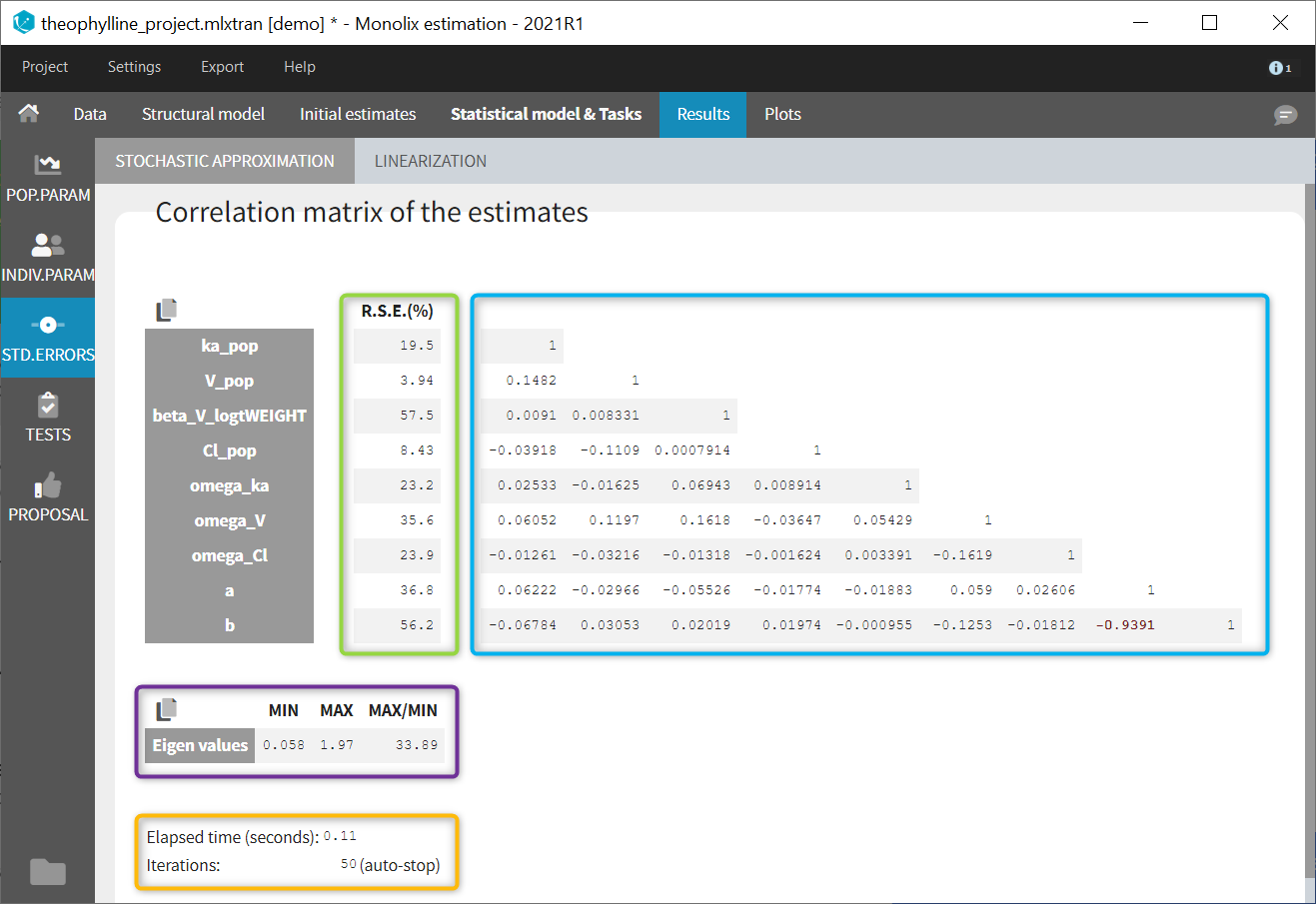
If you hover on a specific value with the mouse, both parameters are highlighted to know easily which parameter you are looking at:

In the output folder

After having run the Standard errors task, the following files are available:

summary.txt: contains the s.e, r.s.e, p-values, correlation matrix and eigenvalues in an easily readable format, as well as elapsed time and number of iterations for stochastic approximation (starting from Monolix2021R1).
populationParameters.txt: contains the s.e, r.s.e and p-values in csv format, for the method with (*_lin) or without (*_sa) linearization
FisherInformation/correlationEstimatesSA.txt: correlation matrix of the population parameter estimates, method without linearization (stochastic approximation)
FisherInformation/correlationEstimatesLin.txt: correlation matrix of the population parameter estimates, method with linearization
FisherInformation/covarianceEstimatesSA.txt: variance-covariance matrix of the transformed normally distributed population parameter, method without linearization (stochastic approximation)
FisherInformation/covarianceEstimatesLin.txt: variance-covariance matrix of the transformed normally distributed population parameter, method with linearization

Interpreting the correlation matrix of the estimates

The color code of Monolix’s results allows to quickly identify population parameter estimates that are strongly correlated. This often reflects model overparameterization and can be further investigated using Mlxplore and the convergence assessment. This is explained in details in this video:

Settings

The settings are accessible through the interface via the button next to the Standard errors task:

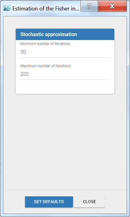
Minimum number of iterations: minimum number of iterations of the stochastic approximation algorithm to calculate the Fisher Information Matrix.
Maximum number of iterations: maximum number of iterations of the stochastic approximation algorithm to calculate the Fisher Information Matrix. The algorithm stops even if the stopping criteria are not met.

Good practices and tips

When to use “use linearization method”?

Firstly, it is only possible to use the linearization method for continuous data. For the linearization is available, this method is generally much faster than without linearization (i.e stochastic approximation) but less precise. The Fisher Information Matrix by model linearization will generally be able to identify the main features of the model. More precise– and time-consuming – estimation procedures such as stochastic approximation will have very limited impact in terms of decisions for these most obvious features. Precise results are required for the final runs where it becomes more important to rigorously defend decisions made to choose the final model and provide precise estimates and diagnosis plots.

I have NANs as results for standard errors for parameter estimates. What should I do? Does it impact the likelihood?

NaNs as standard errors often appear when the model is too complex and some parameters are unidentifiable. They can be seen as an infinitely large standard error.
The likelihood is not affected by NaNs in the standard errors. The estimated population parameters having a NaN as standard error are only very uncertain (infinitely large standard error and thus infinitely large confidence intervals).

Источник

В статистике относительная стандартная ошибка (RSE) равна стандартной ошибке оценки обследования, деленной на оценку обследования, а затем умноженной на 100. Число умножается на 100, чтобы его можно было выразить в процентах. RSE не обязательно представляет какую-либо новую информацию, выходящую за рамки стандартной ошибки, но это может быть лучшим методом представления статистической достоверности.

Относительная стандартная ошибка против стандартной ошибки

Стандартная ошибка определяет, насколько оценка обследования может отличаться от фактической совокупности.Он выражается числом.Напротив, относительная стандартная ошибка (RSE) – это стандартная ошибка, выраженная как часть оценки и обычно отображается в процентах.Оценки с RSE 25% или более подвержены большой ошибке выборки и должны использоваться с осторожностью.

Оценка опроса и стандартная ошибка

Опросы и стандартные ошибки – важнейшие части теории вероятностей и статистики. Статистики используют стандартные ошибки для построения доверительных интервалов на основе своих обследованных данных. Достоверность этих оценок также можно оценить с помощью доверительного интервала. Доверительные интервалы важны для определения достоверности эмпирических тестов и исследований.

Доверительный интервал – это тип интервальной оценки, вычисляемой на основе статистики наблюдаемых данных, которая может содержать истинное значение неизвестного параметра совокупности.Доверительные интервалы представляют собой диапазон, в котором, вероятно, находится значение генеральной совокупности.Они построены с использованием оценки значения генеральной совокупности и связанной с ней стандартной ошибки.Например, вероятность того, что значение генеральной совокупности находится в пределах двух стандартных ошибок оценок, составляет приблизительно 95% (т.е. 19 из 20), поэтому 95% доверительный интервал равен оценке плюс или минус две стандартные ошибки.

С точки зрения непрофессионала, стандартная ошибка выборки данных – это измерение вероятной разницы между выборкой и всей совокупностью. Например, исследование с участием 10 000 взрослых, курящих сигареты, может дать несколько иные статистические результаты, чем при опросе всех возможных курящих сигареты взрослых.

Меньшие ошибки выборки указывают на более надежные результаты. Центральная предельная теорема в умозаключениях статистиков показывает, что большие выборки, как правило, имеют приблизительно нормальное распределение и низкие ошибки выборки.

Стандартное отклонение и стандартная ошибка

Стандартное отклонение набора данных используется для выражения концентрации результатов обследования. Меньшее разнообразие данных приводит к более низкому стандартному отклонению. Чем больше разнообразия, тем выше стандартное отклонение.

Стандартную ошибку иногда путают со стандартным отклонением. Стандартная ошибка фактически относится к стандартному отклонению среднего значения. Стандартное отклонение относится к изменчивости внутри любой данной выборки, тогда как стандартная ошибка – это изменчивость самого распределения выборки.

Относительная стандартная ошибка

Стандартная ошибка – это абсолютная мера между выборочным обследованием и генеральной совокупностью. Относительная стандартная ошибка показывает, велика ли стандартная ошибка по сравнению с результатами; большие относительные стандартные ошибки предполагают, что результаты незначительны. Формула относительной стандартной ошибки:

Источник

В статистике относительная стандартная ошибка или RSE равна стандартной ошибке оценки опроса, деленной на оценку опроса, а затем умножается на 100. Число умножается на 100 так его можно выразить в процентах. RSE не обязательно представляет какую-либо новую информацию за пределами стандартной ошибки, но это может быть превосходный метод представления статистической достоверности.

Оценка и стандартная ошибка

Обследования и стандартные ошибки являются важными частями теории вероятностей и статистики. Статистики используют стандартные ошибки для построения доверительных интервалов из своих опрошенных данных. Доверительные интервалы важны для определения действительности эмпирических тестов и исследований.

В условиях непрофессионала стандартная ошибка выборки данных — это измерение вероятной разницы между выборкой и всей совокупностью. Например, исследование с участием 10 000 взрослых, курящих сигареты, может генерировать несколько иные статистические результаты, чем если бы были опрошены все возможные взрослые курильщики сигарет.

Меньшие ошибки выборки свидетельствуют о более надежных результатах. Центральная предельная теорема в статистических выводах показывает, что большие образцы имеют тенденцию иметь приблизительно нормальные распределения и низкие ошибки выборки.

Стандартное отклонение и стандартная ошибка

Стандартное отклонение набора данных используется для выражения концентрации результатов опроса. Меньшее разнообразие данных приводит к более низкому стандартным отклонениям. Больше разнообразия, вероятно, приведет к более высокому стандартным отклонениям.

Стандартная ошибка иногда путается со стандартным отклонением. Стандартная ошибка на самом деле относится к стандартным отклонениям среднего значения. Стандартное отклонение относится к изменчивости внутри любого данного образца, в то время как стандартная ошибка — это изменчивость самого распределения выборки.

Относительная стандартная ошибка

Стандартная ошибка — это абсолютная величина между выборочным обследованием и общей численностью населения. Относительная стандартная ошибка показывает, является ли стандартная ошибка большой по сравнению с результатами; большие относительные стандартные ошибки предполагают, что результаты не значительны. Формула относительной стандартной ошибки (стандартная ошибка / оценка) x 100.

Источник