Residual square error

$begingroup$

Looking at the Wikipedia definitions of:

Mean Squared Error (MSE)
Residual Sum of Squares (RSS)

It looks to me that

$$text{MSE} = frac{1}{N} text{RSS} = frac{1}{N} sum (f_i -y_i)^2$$

where $N$ is he number of samples and $f_i$ is our estimation of $y_i$.

However, none of the Wikipedia articles mention this relationship. Why? Am I missing something?

asked Oct 23, 2013 at 2:55

$endgroup$

$begingroup$

Actually it’s mentioned in the Regression section of Mean squared error in Wikipedia:

In regression analysis, the term mean squared error is sometimes used
to refer to the unbiased estimate of error variance: the residual sum
of squares divided by the number of degrees of freedom.

You can also find some informations here: Errors and residuals in statistics
It says the expression mean squared error may have different meanings in different cases, which is tricky sometimes.

answered Mar 19, 2014 at 13:05

whenovwhenov

5466 silver badges4 bronze badges

$endgroup$

$begingroup$

But be aware that Sum of Squared Errors (SSE) and Residue Sum of Squares (RSS) sometimes are used interchangeably, thus confusing the readers. For instance, check this URL out.

Strictly speaking from statistic point of views, Errors and Residues are completely different concepts. Errors mainly refer to difference between actual observed sample values and your predicted values, and used mostly in the statistic metrics like Root Means Squared Errors (RMSE) and Mean Absolute Errors (MAE). In contrast, residues refer exclusively to the differences between dependent variables and estimations from linear regression.

answered Jun 16, 2019 at 17:04

Dr.CYYDr.CYY

871 silver badge1 bronze badge

$endgroup$

$begingroup$

I don´t think this is correct here if we consider MSE to be the sqaure of RMSE. For instance, you have a series of sampled data on predictions and observations, now you try to do a linear regresion: Observation (O)= a + b X Prediction (P). In this case, the MSE is the sum of squared difference between O and P and divided by sample size N.

But if you want to measure how linear regression performs, you need to calculate Mean Squared Residue (MSR). In the same case, it would be firstly calculating Residual Sum of Squares (RSS) that corresponds to sum of squared differences between actual observation values and predicted observations derived from the linear regression.Then, it is followed for RSS divided by N-2 to get MSR.

Simply put, in the example, MSE can not be estimated using RSS/N since RSS component is no longer the same for the component used to calculate MSE.

answered Jun 15, 2019 at 18:14

Dr.CYYDr.CYY

871 silver badge1 bronze badge

$endgroup$

Источник

From Wikipedia, the free encyclopedia

In statistics and optimization, errors and residuals are two closely related and easily confused measures of the deviation of an observed value of an element of a statistical sample from its «true value» (not necessarily observable). The error of an observation is the deviation of the observed value from the true value of a quantity of interest (for example, a population mean). The residual is the difference between the observed value and the estimated value of the quantity of interest (for example, a sample mean). The distinction is most important in regression analysis, where the concepts are sometimes called the regression errors and regression residuals and where they lead to the concept of studentized residuals.
In econometrics, «errors» are also called disturbances.^[1]^[2]^[3]

Introduction[edit]

Suppose there is a series of observations from a univariate distribution and we want to estimate the mean of that distribution (the so-called location model). In this case, the errors are the deviations of the observations from the population mean, while the residuals are the deviations of the observations from the sample mean.

A statistical error (or disturbance) is the amount by which an observation differs from its expected value, the latter being based on the whole population from which the statistical unit was chosen randomly. For example, if the mean height in a population of 21-year-old men is 1.75 meters, and one randomly chosen man is 1.80 meters tall, then the «error» is 0.05 meters; if the randomly chosen man is 1.70 meters tall, then the «error» is −0.05 meters. The expected value, being the mean of the entire population, is typically unobservable, and hence the statistical error cannot be observed either.

A residual (or fitting deviation), on the other hand, is an observable estimate of the unobservable statistical error. Consider the previous example with men’s heights and suppose we have a random sample of n people. The sample mean could serve as a good estimator of the population mean. Then we have:

The difference between the height of each man in the sample and the unobservable population mean is a statistical error, whereas
The difference between the height of each man in the sample and the observable sample mean is a residual.

Note that, because of the definition of the sample mean, the sum of the residuals within a random sample is necessarily zero, and thus the residuals are necessarily not independent. The statistical errors, on the other hand, are independent, and their sum within the random sample is almost surely not zero.

One can standardize statistical errors (especially of a normal distribution) in a z-score (or «standard score»), and standardize residuals in a t-statistic, or more generally studentized residuals.

In univariate distributions[edit]

If we assume a normally distributed population with mean μ and standard deviation σ, and choose individuals independently, then we have

${displaystyle X_{1},dots ,X_{n}sim Nleft(mu ,sigma ^{2}right),}$

and the sample mean

$overline{X}={X_1 + cdots + X_n over n}$

is a random variable distributed such that:

${displaystyle {overline {X}}sim Nleft(mu ,{frac {sigma ^{2}}{n}}right).}$

The statistical errors are then

${displaystyle e_{i}=X_{i}-mu ,,}$

with expected values of zero,^[4] whereas the residuals are

${displaystyle r_{i}=X_{i}-{overline {X}}.}$

The sum of squares of the statistical errors, divided by σ², has a chi-squared distribution with n degrees of freedom:

${displaystyle {frac {1}{sigma ^{2}}}sum _{i=1}^{n}e_{i}^{2}sim chi _{n}^{2}.}$

However, this quantity is not observable as the population mean is unknown. The sum of squares of the residuals, on the other hand, is observable. The quotient of that sum by σ² has a chi-squared distribution with only n − 1 degrees of freedom:

${frac 1{sigma ^{2}}}sum _{{i=1}}^{n}r_{i}^{2}sim chi _{{n-1}}^{2}.$

This difference between n and n − 1 degrees of freedom results in Bessel’s correction for the estimation of sample variance of a population with unknown mean and unknown variance. No correction is necessary if the population mean is known.

[edit]

It is remarkable that the sum of squares of the residuals and the sample mean can be shown to be independent of each other, using, e.g. Basu’s theorem. That fact, and the normal and chi-squared distributions given above form the basis of calculations involving the t-statistic:

${displaystyle T={frac {{overline {X}}_{n}-mu _{0}}{S_{n}/{sqrt {n}}}},}$

where ${displaystyle {overline {X}}_{n}-mu _{0}}$ represents the errors, $S_{n}$ represents the sample standard deviation for a sample of size n, and unknown σ, and the denominator term accounts for the standard deviation of the errors according to:^[5]

${displaystyle operatorname {Var} left({overline {X}}_{n}right)={frac {sigma ^{2}}{n}}}$

The probability distributions of the numerator and the denominator separately depend on the value of the unobservable population standard deviation σ, but σ appears in both the numerator and the denominator and cancels. That is fortunate because it means that even though we do not know σ, we know the probability distribution of this quotient: it has a Student’s t-distribution with n − 1 degrees of freedom. We can therefore use this quotient to find a confidence interval for μ. This t-statistic can be interpreted as «the number of standard errors away from the regression line.»^[6]

Regressions[edit]

In regression analysis, the distinction between errors and residuals is subtle and important, and leads to the concept of studentized residuals. Given an unobservable function that relates the independent variable to the dependent variable – say, a line – the deviations of the dependent variable observations from this function are the unobservable errors. If one runs a regression on some data, then the deviations of the dependent variable observations from the fitted function are the residuals. If the linear model is applicable, a scatterplot of residuals plotted against the independent variable should be random about zero with no trend to the residuals.^[5] If the data exhibit a trend, the regression model is likely incorrect; for example, the true function may be a quadratic or higher order polynomial. If they are random, or have no trend, but «fan out» — they exhibit a phenomenon called heteroscedasticity. If all of the residuals are equal, or do not fan out, they exhibit homoscedasticity.

However, a terminological difference arises in the expression mean squared error (MSE). The mean squared error of a regression is a number computed from the sum of squares of the computed residuals, and not of the unobservable errors. If that sum of squares is divided by n, the number of observations, the result is the mean of the squared residuals. Since this is a biased estimate of the variance of the unobserved errors, the bias is removed by dividing the sum of the squared residuals by df = n − p − 1, instead of n, where df is the number of degrees of freedom (n minus the number of parameters (excluding the intercept) p being estimated — 1). This forms an unbiased estimate of the variance of the unobserved errors, and is called the mean squared error.^[7]

Another method to calculate the mean square of error when analyzing the variance of linear regression using a technique like that used in ANOVA (they are the same because ANOVA is a type of regression), the sum of squares of the residuals (aka sum of squares of the error) is divided by the degrees of freedom (where the degrees of freedom equal n − p − 1, where p is the number of parameters estimated in the model (one for each variable in the regression equation, not including the intercept)). One can then also calculate the mean square of the model by dividing the sum of squares of the model minus the degrees of freedom, which is just the number of parameters. Then the F value can be calculated by dividing the mean square of the model by the mean square of the error, and we can then determine significance (which is why you want the mean squares to begin with.).^[8]

However, because of the behavior of the process of regression, the distributions of residuals at different data points (of the input variable) may vary even if the errors themselves are identically distributed. Concretely, in a linear regression where the errors are identically distributed, the variability of residuals of inputs in the middle of the domain will be higher than the variability of residuals at the ends of the domain:^[9] linear regressions fit endpoints better than the middle. This is also reflected in the influence functions of various data points on the regression coefficients: endpoints have more influence.

Thus to compare residuals at different inputs, one needs to adjust the residuals by the expected variability of residuals, which is called studentizing. This is particularly important in the case of detecting outliers, where the case in question is somehow different than the other’s in a dataset. For example, a large residual may be expected in the middle of the domain, but considered an outlier at the end of the domain.

Other uses of the word «error» in statistics[edit]

The use of the term «error» as discussed in the sections above is in the sense of a deviation of a value from a hypothetical unobserved value. At least two other uses also occur in statistics, both referring to observable prediction errors:

The mean squared error (MSE) refers to the amount by which the values predicted by an estimator differ from the quantities being estimated (typically outside the sample from which the model was estimated).
The root mean square error (RMSE) is the square-root of MSE.
The sum of squares of errors (SSE) is the MSE multiplied by the sample size.

Sum of squares of residuals (SSR) is the sum of the squares of the deviations of the actual values from the predicted values, within the sample used for estimation. This is the basis for the least squares estimate, where the regression coefficients are chosen such that the SSR is minimal (i.e. its derivative is zero).

Likewise, the sum of absolute errors (SAE) is the sum of the absolute values of the residuals, which is minimized in the least absolute deviations approach to regression.

The mean error (ME) is the bias.
The mean residual (MR) is always zero for least-squares estimators.

References[edit]

^ Kennedy, P. (2008). A Guide to Econometrics. Wiley. p. 576. ISBN 978-1-4051-8257-7. Retrieved 2022-05-13.
^ Wooldridge, J.M. (2019). Introductory Econometrics: A Modern Approach. Cengage Learning. p. 57. ISBN 978-1-337-67133-0. Retrieved 2022-05-13.
^ Das, P. (2019). Econometrics in Theory and Practice: Analysis of Cross Section, Time Series and Panel Data with Stata 15.1. Springer Singapore. p. 7. ISBN 978-981-329-019-8. Retrieved 2022-05-13.
^ Wetherill, G. Barrie. (1981). Intermediate statistical methods. London: Chapman and Hall. ISBN 0-412-16440-X. OCLC 7779780.
^ ^a ^b A modern introduction to probability and statistics : understanding why and how. Dekking, Michel, 1946-. London: Springer. 2005. ISBN 978-1-85233-896-1. OCLC 262680588.{{cite book}}: CS1 maint: others (link)
^ Bruce, Peter C., 1953- (2017-05-10). Practical statistics for data scientists : 50 essential concepts. Bruce, Andrew, 1958- (First ed.). Sebastopol, CA. ISBN 978-1-4919-5293-1. OCLC 987251007.{{cite book}}: CS1 maint: multiple names: authors list (link)
^ Steel, Robert G. D.; Torrie, James H. (1960). Principles and Procedures of Statistics, with Special Reference to Biological Sciences. McGraw-Hill. p. 288.
^ Zelterman, Daniel (2010). Applied linear models with SAS ([Online-Ausg.]. ed.). Cambridge: Cambridge University Press. ISBN 9780521761598.
^ «7.3: Types of Outliers in Linear Regression». Statistics LibreTexts. 2013-11-21. Retrieved 2019-11-22.

Cook, R. Dennis; Weisberg, Sanford (1982). Residuals and Influence in Regression (Repr. ed.). New York: Chapman and Hall. ISBN 041224280X. Retrieved 23 February 2013.
Cox, David R.; Snell, E. Joyce (1968). «A general definition of residuals». Journal of the Royal Statistical Society, Series B. 30 (2): 248–275. JSTOR 2984505.
Weisberg, Sanford (1985). Applied Linear Regression (2nd ed.). New York: Wiley. ISBN 9780471879572. Retrieved 23 February 2013.
«Errors, theory of», Encyclopedia of Mathematics, EMS Press, 2001 [1994]

External links[edit]

Media related to Errors and residuals at Wikimedia Commons

Источник

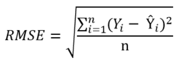
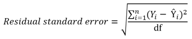
The residual standard error is used to measure how well a regression model fits a dataset.

In simple terms, it measures the standard deviation of the residuals in a regression model.

It is calculated as:

Residual standard error = √Σ(y – ŷ)²/df

where:

y: The observed value
ŷ: The predicted value
df: The degrees of freedom, calculated as the total number of observations – total number of model parameters.

The smaller the residual standard error, the better a regression model fits a dataset. Conversely, the higher the residual standard error, the worse a regression model fits a dataset.

A regression model that has a small residual standard error will have data points that are closely packed around the fitted regression line:

The residuals of this model (the difference between the observed values and the predicted values) will be small, which means the residual standard error will also be small.

Conversely, a regression model that has a large residual standard error will have data points that are more loosely scattered around the fitted regression line:

The residuals of this model will be larger, which means the residual standard error will also be larger.

The following example shows how to calculate and interpret the residual standard error of a regression model in R.

Example: Interpreting Residual Standard Error

Suppose we would like to fit the following multiple linear regression model:

mpg = β₀ + β₁(displacement) + β₂(horsepower)

This model uses the predictor variables “displacement” and “horsepower” to predict the miles per gallon that a given car gets.

The following code shows how to fit this regression model in R:

#load built-in mtcars dataset
data(mtcars)

#fit regression model
model <- lm(mpg~disp+hp, data=mtcars)

#view model summary
summary(model)

Call:
lm(formula = mpg ~ disp + hp, data = mtcars)

Residuals:
    Min      1Q  Median      3Q     Max 
-4.7945 -2.3036 -0.8246  1.8582  6.9363 

Coefficients:
             Estimate Std. Error t value Pr(>|t|)    
(Intercept) 30.735904   1.331566  23.083  < 2e-16 ***
disp        -0.030346   0.007405  -4.098 0.000306 ***
hp          -0.024840   0.013385  -1.856 0.073679 .  
---
Signif. codes:  0 '***' 0.001 '**' 0.01 '*' 0.05 '.' 0.1 ' ' 1

Residual standard error: 3.127 on 29 degrees of freedom
Multiple R-squared:  0.7482,	Adjusted R-squared:  0.7309 
F-statistic: 43.09 on 2 and 29 DF,  p-value: 2.062e-09

Near the bottom of the output we can see that the residual standard error of this model is 3.127.

This tells us that the regression model predicts the mpg of cars with an average error of about 3.127.

Using Residual Standard Error to Compare Models

The residual standard error is particularly useful for comparing the fit of different regression models.

For example, suppose we fit two different regression models to predict the mpg of cars. The residual standard error of each model is as follows:

Residual standard error of model 1: 3.127
Residual standard error of model 2: 5.657

Since model 1 has a lower residual standard error, it fits the data better than model 2. Thus, we would prefer to use model 1 to predict the mpg of cars because the predictions it makes are closer to the observed mpg values of the cars.

Additional Resources

How to Perform Simple Linear Regression in R
How to Perform Multiple Linear Regression in R
How to Create a Residual Plot in R

Источник

Как интерпретировать остаточную стандартную ошибку

17 авг. 2022 г.
читать 2 мин

Остаточная стандартная ошибка используется для измерения того, насколько хорошо модель регрессии соответствует набору данных.

Проще говоря, он измеряет стандартное отклонение остатков в регрессионной модели.

Он рассчитывается как:

Остаточная стандартная ошибка = √ Σ(y – ŷ) 2 /df

куда:

y: наблюдаемое значение
ŷ: Прогнозируемое значение
df: Степени свободы, рассчитанные как общее количество наблюдений – общее количество параметров модели.

Чем меньше остаточная стандартная ошибка, тем лучше регрессионная модель соответствует набору данных. И наоборот, чем выше остаточная стандартная ошибка, тем хуже регрессионная модель соответствует набору данных.

Модель регрессии с небольшой остаточной стандартной ошибкой будет иметь точки данных, которые плотно упакованы вокруг подобранной линии регрессии:

Остатки этой модели (разница между наблюдаемыми значениями и прогнозируемыми значениями) будут малы, что означает, что остаточная стандартная ошибка также будет небольшой.

И наоборот, регрессионная модель с большой остаточной стандартной ошибкой будет иметь точки данных, которые более свободно разбросаны по подобранной линии регрессии:

Остатки этой модели будут больше, что означает, что стандартная ошибка невязки также будет больше.

В следующем примере показано, как рассчитать и интерпретировать остаточную стандартную ошибку регрессионной модели в R.

Пример: интерпретация остаточной стандартной ошибки

Предположим, мы хотели бы подогнать следующую модель множественной линейной регрессии:

миль на галлон = β 0 + β 1 (смещение) + β 2 (лошадиные силы)

Эта модель использует переменные-предикторы «объем двигателя» и «лошадиная сила» для прогнозирования количества миль на галлон, которое получает данный автомобиль.

В следующем коде показано, как подогнать эту модель регрессии в R:

#load built-in *mtcars* dataset
data(mtcars)

#fit regression model
model <- lm(mpg~disp+hp, data=mtcars)

#view model summary
summary(model)

Call:
lm(formula = mpg ~ disp + hp, data = mtcars)

Residuals:
 Min 1Q Median 3Q Max 
-4.7945 -2.3036 -0.8246 1.8582 6.9363 

Coefficients:
 Estimate Std. Error t value Pr(>|t|) 
(Intercept) 30.735904 1.331566 23.083 < 2e-16 ***
disp -0.030346 0.007405 -4.098 0.000306 ***
hp -0.024840 0.013385 -1.856 0.073679.
---
Signif. codes: 0 '***' 0.001 '**' 0.01 '*' 0.05 '.' 0.1 ' ' 1

Residual standard error: 3.127 on 29 degrees of freedom
Multiple R-squared: 0.7482, Adjusted R-squared: 0.7309 
F-statistic: 43.09 on 2 and 29 DF, p-value: 2.062e-09

В нижней части вывода мы видим, что остаточная стандартная ошибка этой модели составляет 3,127 .

Это говорит нам о том, что регрессионная модель предсказывает расход автомобилей на галлон со средней ошибкой около 3,127.

Использование остаточной стандартной ошибки для сравнения моделей

Остаточная стандартная ошибка особенно полезна для сравнения соответствия различных моделей регрессии.

Например, предположим, что мы подогнали две разные регрессионные модели для прогнозирования расхода автомобилей на галлон. Остаточная стандартная ошибка каждой модели выглядит следующим образом:

Остаточная стандартная ошибка модели 1: 3,127
Остаточная стандартная ошибка модели 2: 5,657

Поскольку модель 1 имеет меньшую остаточную стандартную ошибку, она лучше соответствует данным, чем модель 2. Таким образом, мы предпочли бы использовать модель 1 для прогнозирования расхода автомобилей на галлон, потому что прогнозы, которые она делает, ближе к наблюдаемым значениям расхода автомобилей на галлон.

Дополнительные ресурсы

Как выполнить простую линейную регрессию в R
Как выполнить множественную линейную регрессию в R
Как создать остаточный график в R

Источник

$begingroup$

Looking at the Wikipedia definitions of:

Mean Squared Error (MSE)
Residual Sum of Squares (RSS)

It looks to me that

$$text{MSE} = frac{1}{N} text{RSS} = frac{1}{N} sum (f_i -y_i)^2$$

where $N$ is he number of samples and $f_i$ is our estimation of $y_i$.

However, none of the Wikipedia articles mention this relationship. Why? Am I missing something?

asked Oct 23, 2013 at 2:55

$endgroup$

$begingroup$

Actually it’s mentioned in the Regression section of Mean squared error in Wikipedia:

In regression analysis, the term mean squared error is sometimes used
to refer to the unbiased estimate of error variance: the residual sum
of squares divided by the number of degrees of freedom.

You can also find some informations here: Errors and residuals in statistics
It says the expression mean squared error may have different meanings in different cases, which is tricky sometimes.

answered Mar 19, 2014 at 13:05

whenovwhenov

5466 silver badges4 bronze badges

$endgroup$

$begingroup$

But be aware that Sum of Squared Errors (SSE) and Residue Sum of Squares (RSS) sometimes are used interchangeably, thus confusing the readers. For instance, check this URL out.

answered Jun 16, 2019 at 17:04

Dr.CYYDr.CYY

871 silver badge1 bronze badge

$endgroup$

$begingroup$

Simply put, in the example, MSE can not be estimated using RSS/N since RSS component is no longer the same for the component used to calculate MSE.

answered Jun 15, 2019 at 18:14

Dr.CYYDr.CYY

871 silver badge1 bronze badge

$endgroup$

Источник

The residual standard deviation (or residual standard error) is a measure used to assess how well a linear regression model fits the data. (The other measure to assess this goodness of fit is R²).

But before we discuss the residual standard deviation, let’s try to assess the goodness of fit graphically.

Consider the following linear regression model:

Y = β₀ + β₁X + ε

Plotted below are examples of 2 of these regression lines modeling 2 different datasets:

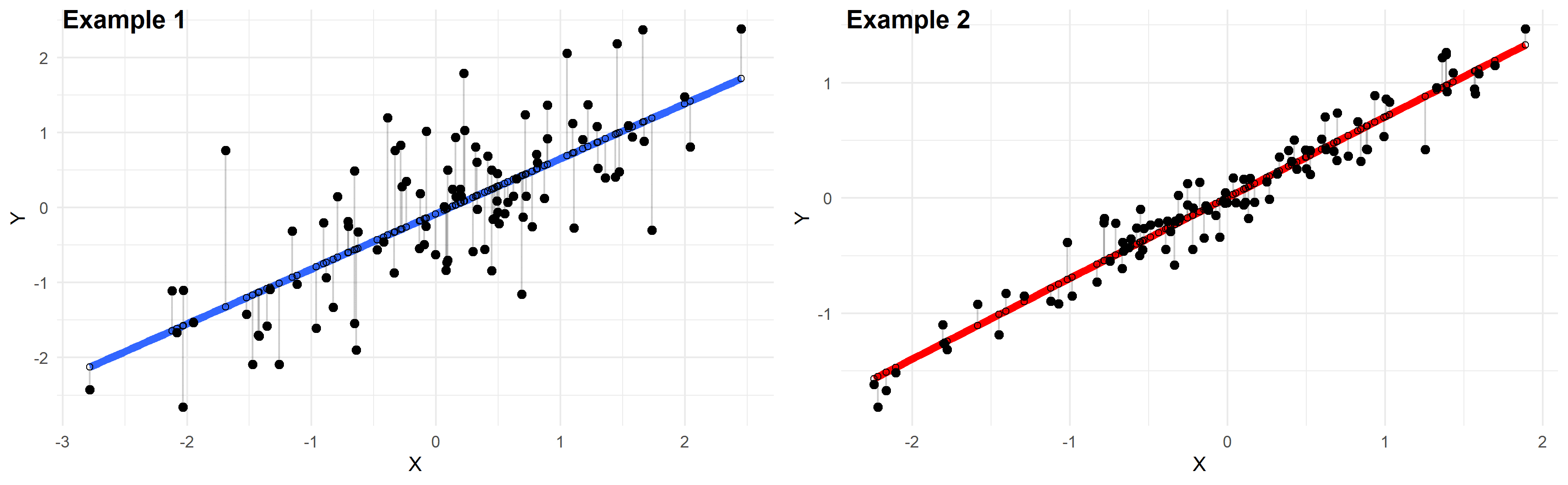
Just by looking at these plots we can say that the linear regression model in “example 2” fits the data better than that of “example 1”.

This is because in “example 2” the points are closer to the regression line. Therefore, using a linear regression model to approximate the true values of these points will yield smaller errors than “example 1”.

In the plots above, the gray vertical lines represent the error terms — the difference between the model and the true value of Y.

Mathematically, the error of the i^th point on the x-axis is given by the equation: (Y_i – Ŷ_i), which is the difference between the true value of Y (Y_i) and the value predicted by the linear model (Ŷ_i) — this difference determines the length of the gray vertical lines in the plots above.

Now that we developed a basic intuition, next we will try to come up with a statistic that quantifies this goodness of fit.

Residual standard deviation vs residual standard error vs RMSE

The simplest way to quantify how far the data points are from the regression line, is to calculate the average distance from this line:

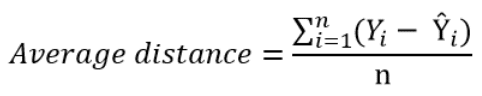
Where n is the sample size.

But, because some of the distances are positive and some are negative (certain points are above the regression line and others are below it), these distances will cancel each other out — meaning that the average distance will be biased low.

In order to remedy this situation, one solution is to take the square of this distance (which will always be a positive number), then calculate the sum of these squared distances for all data points and finally take the square root of this sum to obtain the Root Mean Square Error (RMSE):

We can take this equation one step further:

Instead of dividing by the sample size n, we can divide by the degrees of freedom df to obtain an unbiased estimation of the standard deviation of the error term ε. (If you’re having trouble with this idea, I recommend these 4 videos from Khan Academy which provide a simple explanation mainly through simulations instead of math equations).

The quantity obtained is sometimes called the residual standard deviation (as referred to it in the textbook Data Analysis Using Regression and Multilevel Hierarchical Models by Andrew Gelman and Jennifer Hill). Other textbooks refer to it as the residual standard error (for example An Introduction to Statistical Learning by Gareth James, Daniela Witten, Trevor Hastie and Robert Tibshirani).

In the statistical programming language R, calling the function summary on the linear model will calculate it automatically.

The degrees of freedom df are the sample size minus the number of parameters we’re trying to estimate.

For example, if we’re estimating 2 parameters β₀ and β₁ as in:

Y = β₀ + β₁X + ε

Then, df = n – 2

If we’re estimating 3 parameters, as in:

Y = β₀ + β₁X₁ + β₂X₂ + ε

Then, df = n – 3

And so on…

Now that we have a statistic that measures the goodness of fit of a linear model, next we will discuss how to interpret it in practice.

How to interpret the residual standard deviation/error

Simply put, the residual standard deviation is the average amount that the real values of Y differ from the predictions provided by the regression line.

We can divide this quantity by the mean of Y to obtain the average deviation in percent (which is useful because it will be independent of the units of measure of Y).

Here’s an example:

Suppose we regressed systolic blood pressure (SBP) onto body mass index (BMI) — which is a fancy way of saying that we ran the following linear regression model:

SBP = β₀ + β₁×BMI + ε

After running the model we found that:

β₀ = 100
β1 = 1
And the residual standard error is 12 mmHg

So we can say that the BMI accurately predicts systolic blood pressure with about 12 mmHg error on average.

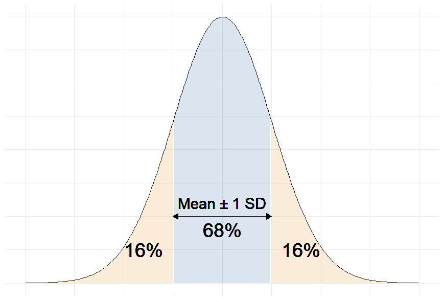
More precisely, we can say that 68% of the predicted SBP values will be within ∓ 12 mmHg of the real values.

Why 68%?

Remember that in linear regression, the error terms are Normally distributed.

And one of the properties of the Normal distribution is that 68% of the data sits around 1 standard deviation from the average (See figure below).

Therefore, 68% of the errors will be between ∓ 1 × residual standard deviation.

For example, our linear regression equation predicts that a person with a BMI of 20 will have an SBP of:

SBP = β₀ + β₁×BMI = 100 + 1 × 20 = 120 mmHg.

With a residual error of 12 mmHg, this person has a 68% chance of having his true SBP between 108 and 132 mmHg.

Moreover, if the mean of SBP in our sample is 130 mmHg for example, then:

12 mmHg ÷ 130 mmHg = 9.2%

So we can also say that the BMI accurately predicts systolic blood pressure with a percentage error of 9.2%.

The question remains: Is 9.2% a good percent error value? More generally, what is a good value for the residual standard deviation?

The answer is that there is no universally acceptable threshold for the residual standard deviation. This should be decided based on your experience in the domain.

In general, the smaller the residual standard deviation/error, the better the model fits the data. And if the value is deemed unacceptably large, consider using a model other than linear regression.

Video transcript

— [Instructor] What we’re
going to do in this video is calculate a typical measure of how well the actual data points agree with a model, in
this case, a linear model and there’s several names for it. We could consider this to
be the standard deviation of the residuals and that’s essentially what
we’re going to calculate. You could also call it
the root-mean-square error and you’ll see why it’s called this because this really describes
how we calculate it. So, what we’re going to do is look at the residuals
for each of these points and then we’re going to find
the standard deviation of them. So, just as a bit of review, the ith residual is going to
be equal to the ith Y value for a given X minus the predicted Y value for a given X. Now, when I say Y hat right over here, this just says what would
the linear regression predict for a given X? And this is the actual Y for a given X. So, for example, and we’ve
done this in other videos, this is all review, the residual here when X is equal to one, we have Y is equal to one but what was predicted by the model is 2.5 times one minus two which is .5. So, one minus .5, so this residual here, this residual is equal to one minus 0.5 which is equal to 0.5 and it’s a positive 0.5 and if the actual point is above the model you’re going to have a positive residual. Now, the residual over here you also have the actual point
being higher than the model, so this is also going to
be a positive residual and once again, when X is equal to three, the actual Y is six, the predicted Y is 2.5 times three, which is 7.5 minus two which is 5.5. So, you have six minus 5.5, so here I’ll write residual
is equal to six minus 5.5 which is equal to 0.5. So, once again you have
a positive residual. Now, for this point that
sits right on the model, the actual is the predicted, when X is two, the actual is three and what was predicted
by the model is three, so the residual here is
equal to the actual is three and the predicted is three, so it’s equal to zero and then last but not least, you have this data point where the residual is
going to be the actual, when X is equal to two is two, minus the predicted. Well, when X is equal to two, you have 2.5 times two, which is equal to five
minus two is equal to three. So, two minus three is
equal to negative one. And so, when your actual is
below your regression line, you’re going to have a negative residual, so this is going to be
negative one right over there. Now we can calculate
the standard deviation of the residuals. We’re going to take this first residual which is 0.5, and we’re going to square it, we’re going to add it
to the second residual right over here, I’ll use
this blue or this teal color, that’s zero, gonna square that. Then we have this third
residual which is negative one, so plus negative one squared and then finally, we
have that fourth residual which is 0.5 squared, 0.5 squared, so once again, we took
each of the residuals, which you could view as the distance between the points and what
the model would predict, we are squaring them, when you take a typical
standard deviation, you’re taking the distance
between a point and the mean. Here we’re taking the
distance between a point and what the model would have predicted but we’re squaring each of those residuals and adding them all up together, and just like we do with the
sample standard deviation, we are now going to divide by one less than the number of residuals
we just squared and added, so we have four residuals, we’re going to divide by four minus one which is equal to of course three. You could view this part as
a mean of the squared errors and now we’re gonna take
the square root of it. So, let’s see, this is going
to be equal to square root of this is 0.25, 0.25, this is just zero, this is going to be positive one, and then this 0.5 squared is going to be 0.25, 0.25, all of that over three. Now, this numerator is going to be 1.5 over three, so this is
going to be equal to, 1.5 is exactly half of three, so we could say this is equal to the square root of one half, this one over the square root of two, one divided by the square root of two which gets us to, so if we round to the nearest thousandths, it’s roughly 0.707. So, approximately 0.707. And if you wanted to visualize that, one standard deviation of
the residuals below the line would look like this, and one standard deviation above the line for any given X value would
go one standard deviation of the residuals above it, it would look something like that. And this is obviously just
a hand-drawn approximation but you do see that this does
seem to be roughly indicative of the typical residual. Now, it’s worth noting, sometimes people will say
it’s the average residual and it depends how you
think about the word average because we are squaring the residuals, so outliers, things that are
really far from the line, when you square it are going to have disproportionate impact here. If you didn’t want to have that behavior we could have done
something like find the mean of the absolute residuals, that actually in some ways
would have been the simple one but this is a standard way of
people trying to figure out how much a model disagrees
with the actual data, and so you can imagine
the lower this number is the better the fit of the model.

Источник

Introduction[edit]

In univariate distributions[edit]

[edit]

Regressions[edit]

Other uses of the word «error» in statistics[edit]

See also[edit]

References[edit]

External links[edit]

Example: Interpreting Residual Standard Error

Using Residual Standard Error to Compare Models

Additional Resources

Как интерпретировать остаточную стандартную ошибку

Пример: интерпретация остаточной стандартной ошибки

Использование остаточной стандартной ошибки для сравнения моделей

Дополнительные ресурсы

Residual standard deviation vs residual standard error vs RMSE

How to interpret the residual standard deviation/error

Further reading

Video transcript