Оценка результатов линейной регрессии
Время прочтения
6 мин
Просмотры 91K
Введение
Сегодня уже все, кто хоть немного интересуется дата майнингом, наверняка слышали про простую линейную регрессию. Про нее уже писали на хабре, а также подробно рассказывал Эндрю Нг в своем известном курсе машинного обучения. Линейная регрессия является одним из базовых и самых простых методов машинного обучения, однако очень редко упоминаются методы оценки качества построенной модели. В этой статье я постараюсь немного исправить это досадное упущение на примере разбора результатов функции summary.lm() в языке R. При этом я постараюсь предоставить необходимые формулы, таким образом все вычисления можно легко запрограммировать на любом другом языке. Эта статья предназначена для тех, кто слышал о том, что можно строить линейную регрессию, но не сталкивался со статистическими процедурами для оценки ее качества.
Модель линейной регрессии
Итак, пусть есть несколько независимых случайных величин X1, X2, …, Xn (предикторов) и зависящая от них величина Y (предполагается, что все необходимые преобразования предикторов уже сделаны). Более того, мы предполагаем, что зависимость линейная, а ошибки рапределены нормально, то есть

где I — единичная квадратная матрица размера n x n.
Итак, у нас есть данные, состоящие из k наблюдений величин Y и Xi и мы хотим оценить коэффициенты. Стандартным методом для нахождения оценок коэффициентов является метод наименьших квадратов. И аналитическое решение, которое можно получить, применив этот метод, выглядит так:
где b с крышкой — оценка вектора коэффициентов, y — вектор значений зависимой величины, а X — матрица размера k x n+1 (n — количество предикторов, k — количество наблюдений), у которой первый столбец состоит из единиц, второй — значения первого предиктора, третий — второго и так далее, а строки соответствуют имеющимся наблюдениям.
Функция summary.lm() и оценка получившихся результатов
Теперь рассмотрим пример построения модели линейной регрессии в языке R:
> library(faraway)
> lm1<-lm(Species~Area+Elevation+Nearest+Scruz+Adjacent, data=gala)
> summary(lm1)

Call:
lm(formula = Species ~ Area + Elevation + Nearest + Scruz + Adjacent,
    data = gala)

Residuals:
     Min       1Q   Median       3Q      Max
-111.679  -34.898   -7.862   33.460  182.584

Coefficients:
             Estimate Std. Error t value Pr(>|t|)
(Intercept)  7.068221  19.154198   0.369 0.715351
Area        -0.023938   0.022422  -1.068 0.296318
Elevation    0.319465   0.053663   5.953 3.82e-06 ***
Nearest      0.009144   1.054136   0.009 0.993151
Scruz       -0.240524   0.215402  -1.117 0.275208
Adjacent    -0.074805   0.017700  -4.226 0.000297 ***
---
Signif. codes:  0 ‘***’ 0.001 ‘**’ 0.01 ‘*’ 0.05 ‘.’ 0.1 ‘ ’ 1

Residual standard error: 60.98 on 24 degrees of freedom
Multiple R-squared:  0.7658,	Adjusted R-squared:  0.7171
F-statistic:  15.7 on 5 and 24 DF,  p-value: 6.838e-07
Таблица gala содержит некоторые данные о 30 Галапагосских островах. Мы будем рассматривать модель, где Species — количество разных видов растений на острове линейно зависит от нескольких других переменных.
Рассмотрим вывод функции summary.lm().
Сначала идет строка, которая напоминает, как строилась модель.
Затем идет информация о распределении остатков: минимум, первая квартиль, медиана, третья квартиль, максимум. В этом месте было бы полезно не только посмотреть на некоторые квантили остатков, но и проверить их на нормальность, например тестом Шапиро-Уилка.
Далее — самое интересное — информация о коэффициентах. Здесь потребуется немного теории.
Сначала выпишем следующий результат:

при этом сигма в квадрате с крышкой является несмещенной оценкой для реальной сигмы в квадрате. Здесь b — реальный вектор коэффициентов, а эпсилон с крышкой — вектор остатков, если в качестве коэффициентов взять оценки, полученные методом наименьших квадратов. То есть при предположении, что ошибки распределены нормально, вектор коэффициентов тоже будет распределен нормально вокруг реального значения, а его дисперсию можно несмещенно оценить. Это значит, что можно проверять гипотезу на равенство коэффициентов нулю, а следовательно проверять значимость предикторов, то есть действительно ли величина Xi сильно влияет на качество построенной модели.
Для проверки этой гипотезы нам понадобится следующая статистика, имеющая распределение Стьюдента в том случае, если реальное значение коэффициента bi равно 0:
где
 — стандартная ошибка оценки коэффициента, а t(k-n-1) — распределение Стьюдента с k-n-1 степенями свободы.
Теперь все готово для продолжения разбора вывода функции summary.lm().
Итак, далее идут оценки коэффициентов, полученные методом наименьших квадратов, их стандартные ошибки, значения t-статистики и p-значения для нее. Обычно p-значение сравнивается с каким-нибудь достаточно малым заранее выбранным порогом, например 0.05 или 0.01. И если значение p-статистики оказывается меньше порога, то гипотеза отвергается, если же больше, ничего конкретного, к сожалению, сказать нельзя. Напомню, что в данном случае, так как распределение Стьюдента симметричное относительно 0, то p-значение будет равно 1-F(|t|)+F(-|t|), где F — функция распределения Стьюдента с k-n-1 степенями свободы. Также, R любезно обозначает звездочками значимые коэффициенты, для которых p-значение достаточно мало. То есть, те коэффициенты, которые с очень малой вероятностью равны 0. В строке Signif. codes как раз содержится расшифровка звездочек: если их три, то p-значение от 0 до 0.001, если две, то оно от 0.001 до 0.01 и так далее. Если никаких значков нет, то р-значение больше 0.1.
В нашем примере можно с большой уверенностью сказать, что предикторы Elevation и Adjacent действительно с большой вероятностью влияют на величину Species, а вот про остальные предикторы ничего определенного сказать нельзя. Обычно, в таких случаях предикторы убирают по одному и смотрят, насколько изменяются другие показатели модели, например BIC или Adjusted R-squared, который будет разобран далее.
Значение Residual standart error соответствует просто оценке сигмы с крышкой, а степени свободы вычисляются как k-n-1.
А теперь самая важные статистики, на которые в первую очередь стоит смотреть: R-squared и Adjusted R-squared:

где Yi — реальные значения Y в каждом наблюдении, Yi с крышкой — значения, предсказанные моделью, Y с чертой — среднее по всем реальным значениям Yi.
Начнем со статистики R-квадрат или, как ее иногда называют, коэффициента детерминации. Она показывает, насколько условная дисперсия модели отличается от дисперсии реальных значений Y. Если этот коэффициент близок к 1, то условная дисперсия модели достаточно мала и весьма вероятно, что модель неплохо описывает данные. Если же коэффициент R-квадрат сильно меньше, например, меньше 0.5, то, с большой долей уверенности модель не отражает реальное положение вещей.
Однако, у статистики R-квадрат есть один серьезный недостаток: при увеличении числа предикторов эта статистика может только возрастать. Поэтому, может показаться, что модель с большим количеством предикторов лучше, чем модель с меньшим, даже если все новые предикторы никак не влияют на зависимую переменную. Тут можно вспомнить про принцип бритвы Оккама. Следуя ему, по возможности, стоит избавляться от лишних предикторов в модели, поскольку она становится более простой и понятной. Для этих целей была придумана статистика скорректированный R-квадрат. Она представляет собой обычный R-квадрат, но со штрафом за большое количество предикторов. Основная идея: если новые независимые переменные дают большой вклад в качество модели, значение этой статистики растет, если нет — то наоборот уменьшается.
Для примера рассмотрим ту же модель, что и раньше, но теперь вместо пяти предикторов оставим два:
> lm2<-lm(Species~Elevation+Adjacent, data=gala)
> summary(lm2)

Call:
lm(formula = Species ~ Elevation + Adjacent, data = gala)

Residuals:
    Min      1Q  Median      3Q     Max
-103.41  -34.33  -11.43   22.57  203.65

Coefficients:
            Estimate Std. Error t value Pr(>|t|)
(Intercept)  1.43287   15.02469   0.095 0.924727
Elevation    0.27657    0.03176   8.707 2.53e-09 ***
Adjacent    -0.06889    0.01549  -4.447 0.000134 ***
---
Signif. codes:  0 ‘***’ 0.001 ‘**’ 0.01 ‘*’ 0.05 ‘.’ 0.1 ‘ ’ 1

Residual standard error: 60.86 on 27 degrees of freedom
Multiple R-squared:  0.7376,	Adjusted R-squared:  0.7181
F-statistic: 37.94 on 2 and 27 DF,  p-value: 1.434e-08
Как можно увидеть, значение статистики R-квадрат снизилось, однако значение скорректированного R-квадрат даже немного возросло.
Теперь проверим гипотезу о равенстве нулю всех коэффициентов при предикторах. То есть, гипотезу о том, зависит ли вообще величина Y от величин Xi линейно. Для этого можно использовать следующую статистику, которая, если гипотеза о равенстве нулю всех коэффициентов верна, имеет распределение Фишера c n и k-n-1 степенями свободы:

Значение F-статистики и p-значение для нее находятся в последней строке вывода функции summary.lm().
Заключение
В этой статье были описаны стандартные методы оценки значимости коэффициентов и некоторые критерии оценки качества построенной линейной модели. К сожалению, я не касался вопроса рассмотрения распределения остатков и проверки его на нормальность, поскольку это увеличило бы статью еще вдвое, хотя это и достаточно важный элемент проверки адекватности модели.
Очень надеюсь что мне удалось немного расширить стандартное представление о линейной регрессии, как об алгоритме который просто оценивает некоторый вид зависимости, и показать, как можно оценить его результаты.
The residual standard error is used to measure how well a regression model fits a dataset.
In simple terms, it measures the standard deviation of the residuals in a regression model.
It is calculated as:
Residual standard error = √Σ(y – ŷ)2/df
where:
- y: The observed value
- ŷ: The predicted value
- df: The degrees of freedom, calculated as the total number of observations – total number of model parameters.
The smaller the residual standard error, the better a regression model fits a dataset. Conversely, the higher the residual standard error, the worse a regression model fits a dataset.
A regression model that has a small residual standard error will have data points that are closely packed around the fitted regression line:

The residuals of this model (the difference between the observed values and the predicted values) will be small, which means the residual standard error will also be small.
Conversely, a regression model that has a large residual standard error will have data points that are more loosely scattered around the fitted regression line:

The residuals of this model will be larger, which means the residual standard error will also be larger.
The following example shows how to calculate and interpret the residual standard error of a regression model in R.
Example: Interpreting Residual Standard Error
Suppose we would like to fit the following multiple linear regression model:
mpg = β0 + β1(displacement) + β2(horsepower)
This model uses the predictor variables “displacement” and “horsepower” to predict the miles per gallon that a given car gets.
The following code shows how to fit this regression model in R:
#load built-in mtcars dataset
data(mtcars)

#fit regression model
model <- lm(mpg~disp+hp, data=mtcars)

#view model summary
summary(model)

Call:
lm(formula = mpg ~ disp + hp, data = mtcars)

Residuals:
    Min      1Q  Median      3Q     Max
-4.7945 -2.3036 -0.8246  1.8582  6.9363

Coefficients:
             Estimate Std. Error t value Pr(>|t|)
(Intercept) 30.735904   1.331566  23.083  < 2e-16 ***
disp        -0.030346   0.007405  -4.098 0.000306 ***
hp          -0.024840   0.013385  -1.856 0.073679 .
---
Signif. codes:  0 '***' 0.001 '**' 0.01 '*' 0.05 '.' 0.1 ' ' 1

Residual standard error: 3.127 on 29 degrees of freedom
Multiple R-squared:  0.7482,	Adjusted R-squared:  0.7309
F-statistic: 43.09 on 2 and 29 DF,  p-value: 2.062e-09
Near the bottom of the output we can see that the residual standard error of this model is 3.127.
This tells us that the regression model predicts the mpg of cars with an average error of about 3.127.
Using Residual Standard Error to Compare Models
The residual standard error is particularly useful for comparing the fit of different regression models.
For example, suppose we fit two different regression models to predict the mpg of cars. The residual standard error of each model is as follows:
- Residual standard error of model 1: 3.127
- Residual standard error of model 2: 5.657
Since model 1 has a lower residual standard error, it fits the data better than model 2. Thus, we would prefer to use model 1 to predict the mpg of cars because the predictions it makes are closer to the observed mpg values of the cars.
Additional Resources
How to Perform Simple Linear Regression in R
How to Perform Multiple Linear Regression in R
How to Create a Residual Plot in R
The residual standard deviation (or residual standard error) is a measure used to assess how well a linear regression model fits the data. (The other measure to assess this goodness of fit is R2).
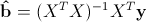
But before we discuss the residual standard deviation, let’s try to assess the goodness of fit graphically.
Consider the following linear regression model:
Y = β0 + β1X + ε
Plotted below are examples of 2 of these regression lines modeling 2 different datasets:
Just by looking at these plots we can say that the linear regression model in “example 2” fits the data better than that of “example 1”.
This is because in “example 2” the points are closer to the regression line. Therefore, using a linear regression model to approximate the true values of these points will yield smaller errors than “example 1”.
In the plots above, the gray vertical lines represent the error terms — the difference between the model and the true value of Y.
Mathematically, the error of the ith point on the x-axis is given by the equation: (Yi – Ŷi), which is the difference between the true value of Y (Yi) and the value predicted by the linear model (Ŷi) — this difference determines the length of the gray vertical lines in the plots above.
Now that we developed a basic intuition, next we will try to come up with a statistic that quantifies this goodness of fit.
Residual standard deviation vs residual standard error vs RMSE
The simplest way to quantify how far the data points are from the regression line, is to calculate the average distance from this line:
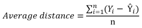
Where n is the sample size.
But, because some of the distances are positive and some are negative (certain points are above the regression line and others are below it), these distances will cancel each other out — meaning that the average distance will be biased low.
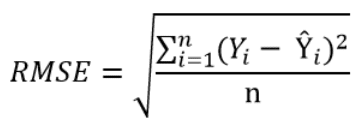
In order to remedy this situation, one solution is to take the square of this distance (which will always be a positive number), then calculate the sum of these squared distances for all data points and finally take the square root of this sum to obtain the Root Mean Square Error (RMSE):
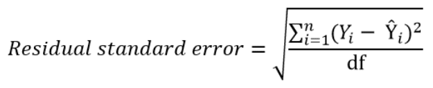
We can take this equation one step further:
Instead of dividing by the sample size n, we can divide by the degrees of freedom df to obtain an unbiased estimation of the standard deviation of the error term ε. (If you’re having trouble with this idea, I recommend these 4 videos from Khan Academy which provide a simple explanation mainly through simulations instead of math equations).
The quantity obtained is sometimes called the residual standard deviation (as referred to it in the textbook Data Analysis Using Regression and Multilevel Hierarchical Models by Andrew Gelman and Jennifer Hill). Other textbooks refer to it as the residual standard error (for example An Introduction to Statistical Learning by Gareth James, Daniela Witten, Trevor Hastie and Robert Tibshirani).
In the statistical programming language R, calling the function summary on the linear model will calculate it automatically.
The degrees of freedom df are the sample size minus the number of parameters we’re trying to estimate.
For example, if we’re estimating 2 parameters β0 and β1 as in:
Y = β0 + β1X + ε
Then, df = n – 2
If we’re estimating 3 parameters, as in:
Y = β0 + β1X1 + β2X2 + ε
Then, df = n – 3
And so on…
Now that we have a statistic that measures the goodness of fit of a linear model, next we will discuss how to interpret it in practice.
How to interpret the residual standard deviation/error
Simply put, the residual standard deviation is the average amount that the real values of Y differ from the predictions provided by the regression line.
We can divide this quantity by the mean of Y to obtain the average deviation in percent (which is useful because it will be independent of the units of measure of Y).
Here’s an example:
Suppose we regressed systolic blood pressure (SBP) onto body mass index (BMI) — which is a fancy way of saying that we ran the following linear regression model:
SBP = β0 + β1×BMI + ε
After running the model we found that:
- β0 = 100
- β1 = 1
- And the residual standard error is 12 mmHg
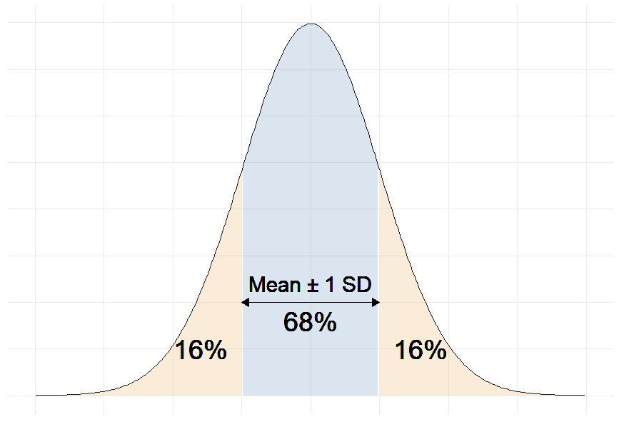
So we can say that the BMI accurately predicts systolic blood pressure with about 12 mmHg error on average.
More precisely, we can say that 68% of the predicted SBP values will be within ∓ 12 mmHg of the real values.
Why 68%?
Remember that in linear regression, the error terms are Normally distributed.
And one of the properties of the Normal distribution is that 68% of the data sits around 1 standard deviation from the average (See figure below).
Therefore, 68% of the errors will be between ∓ 1 × residual standard deviation.
For example, our linear regression equation predicts that a person with a BMI of 20 will have an SBP of:
SBP = β0 + β1×BMI = 100 + 1 × 20 = 120 mmHg.
With a residual error of 12 mmHg, this person has a 68% chance of having his true SBP between 108 and 132 mmHg.
Moreover, if the mean of SBP in our sample is 130 mmHg for example, then:
12 mmHg ÷ 130 mmHg = 9.2%
So we can also say that the BMI accurately predicts systolic blood pressure with a percentage error of 9.2%.
The question remains: Is 9.2% a good percent error value? More generally, what is a good value for the residual standard deviation?
The answer is that there is no universally acceptable threshold for the residual standard deviation. This should be decided based on your experience in the domain.
In general, the smaller the residual standard deviation/error, the better the model fits the data. And if the value is deemed unacceptably large, consider using a model other than linear regression.
Further reading
- What is a Good R-Squared Value? [Based on Real-World Data]
- Understand the F-Statistic in Linear Regression
- Relationship Between r and R-squared in Linear Regression
- Variables to Include in a Regression Model
- 7 Tricks to Get Statistically Significant p-Values
Как интерпретировать остаточную стандартную ошибку
17 авг. 2022 г.
читать 2 мин
Остаточная стандартная ошибка используется для измерения того, насколько хорошо модель регрессии соответствует набору данных.
Проще говоря, он измеряет стандартное отклонение остатков в регрессионной модели.
Он рассчитывается как:
Остаточная стандартная ошибка = √ Σ(y – ŷ) 2 /df
куда:
- y: наблюдаемое значение
- ŷ: Прогнозируемое значение
- df: Степени свободы, рассчитанные как общее количество наблюдений – общее количество параметров модели.
Чем меньше остаточная стандартная ошибка, тем лучше регрессионная модель соответствует набору данных. И наоборот, чем выше остаточная стандартная ошибка, тем хуже регрессионная модель соответствует набору данных.
Модель регрессии с небольшой остаточной стандартной ошибкой будет иметь точки данных, которые плотно упакованы вокруг подобранной линии регрессии:
Остатки этой модели (разница между наблюдаемыми значениями и прогнозируемыми значениями) будут малы, что означает, что остаточная стандартная ошибка также будет небольшой.
И наоборот, регрессионная модель с большой остаточной стандартной ошибкой будет иметь точки данных, которые более свободно разбросаны по подобранной линии регрессии:
Остатки этой модели будут больше, что означает, что стандартная ошибка невязки также будет больше.
В следующем примере показано, как рассчитать и интерпретировать остаточную стандартную ошибку регрессионной модели в R.
Пример: интерпретация остаточной стандартной ошибки
Предположим, мы хотели бы подогнать следующую модель множественной линейной регрессии:
миль на галлон = β 0 + β 1 (смещение) + β 2 (лошадиные силы)
Эта модель использует переменные-предикторы «объем двигателя» и «лошадиная сила» для прогнозирования количества миль на галлон, которое получает данный автомобиль.
В следующем коде показано, как подогнать эту модель регрессии в R:
#load built-in *mtcars* dataset
data(mtcars)

#fit regression model
model <- lm(mpg~disp+hp, data=mtcars)

#view model summary
summary(model)

Call:
lm(formula = mpg ~ disp + hp, data = mtcars)

Residuals:
 Min 1Q Median 3Q Max
-4.7945 -2.3036 -0.8246 1.8582 6.9363

Coefficients:
 Estimate Std. Error t value Pr(>|t|)
(Intercept) 30.735904 1.331566 23.083 < 2e-16 ***
disp -0.030346 0.007405 -4.098 0.000306 ***
hp -0.024840 0.013385 -1.856 0.073679.
---
Signif. codes: 0 '***' 0.001 '**' 0.01 '*' 0.05 '.' 0.1 ' ' 1

Residual standard error: 3.127 on 29 degrees of freedom
Multiple R-squared: 0.7482, Adjusted R-squared: 0.7309
F-statistic: 43.09 on 2 and 29 DF, p-value: 2.062e-09
В нижней части вывода мы видим, что остаточная стандартная ошибка этой модели составляет 3,127 .
Это говорит нам о том, что регрессионная модель предсказывает расход автомобилей на галлон со средней ошибкой около 3,127.
Использование остаточной стандартной ошибки для сравнения моделей
Остаточная стандартная ошибка особенно полезна для сравнения соответствия различных моделей регрессии.
Например, предположим, что мы подогнали две разные регрессионные модели для прогнозирования расхода автомобилей на галлон. Остаточная стандартная ошибка каждой модели выглядит следующим образом:
- Остаточная стандартная ошибка модели 1: 3,127
- Остаточная стандартная ошибка модели 2: 5,657
Поскольку модель 1 имеет меньшую остаточную стандартную ошибку, она лучше соответствует данным, чем модель 2. Таким образом, мы предпочли бы использовать модель 1 для прогнозирования расхода автомобилей на галлон, потому что прогнозы, которые она делает, ближе к наблюдаемым значениям расхода автомобилей на галлон.
Дополнительные ресурсы
Как выполнить простую линейную регрессию в R
Как выполнить множественную линейную регрессию в R
Как создать остаточный график в R
В сообщении «Каков возраст Вселенной?» был приведен пример построения простой линейной регрессии при помощи функции lm(). Полученная в том примере оценка коэффициента регрессии оказалась статистически значимой, что, казалось бы, указывает на высокое качество модели. Но так ли это? В данном сообщении будут рассмотрены количественные показатели, позволяющие ответить на этот вопрос.
F-критерий
В ходе построения модели, отражающей зависимость между расстоянием до 24 галактик и скоростью их удаления, были получены следующие результаты:
library(gamair)
data(hubble)

M <- lm(y ~ x - 1, data = hubble)

summary(M)

Call:
lm(formula = y ~ x - 1, data = hubble)

Residuals:
   Min     1Q Median     3Q    Max
-736.5 -132.5  -19.0  172.2  558.0

Coefficients:
  Estimate Std. Error t value Pr(>|t|)
x   76.581      3.965   19.32 1.03e-15 ***
---
Signif. codes:  0 ‘***’ 0.001 ‘**’ 0.01 ‘*’ 0.05 ‘.’ 0.1 ‘ ’ 1

Residual standard error: 258.9 on 23 degrees of freedom
Multiple R-squared:  0.9419, Adjusted R-squared:  0.9394
F-statistic: 373.1 on 1 and 23 DF,  p-value: 1.032e-15
В последней строке приведенных результатов мы видим значение F-критерия и соответствующее ему Р-значение. Ранее F-критерий был описан в контексте дисперсионного анализа. Что же он делает здесь — в регрессионном анализе? Дело в том, что и дисперсионный анализ, и линейная регрессия с математической точки зрения очень похожи — они являются частными случаями класса «общих линейных моделей» (см. соответствующее обсуждение этой темы в приложении к дисперсионному анализу здесь и здесь). В случае с дисперсионным анализом, мы использовали F-критерий для сравнения меж- и внутригрупповой дисперсий. В случае с регрессионными моделями F-критерий также используется для сравнения дисперсий и рассчитывается следующим образом:
[F = frac{(TSS-RSS)/p}{RSS/(n-p-1)},]
где (TSS=sum (y_i-bar{y})) — т.н. общая сумма квадратов (англ. total sum of squares), (RSS = sum (y_i-hat{y})) — сумма квадратов остатков, (p) — число параметров модели (в нашем случае их два — коэффициент регрессии и стандартное отклонение остатков), а (n) — объем выборки. Приведенный ниже рисунок иллюстрирует, что собой представляют значения (TSS) и (RSS).
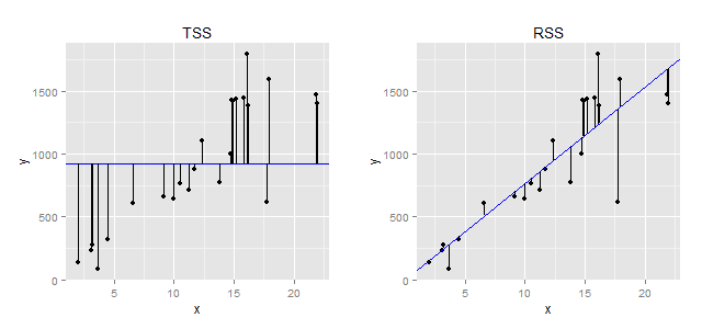 |
| Геометрическая интерпретация понятий «общая сумма квадратов» (TSS) и «сумма квадратов остатков» (RSS). Слева: Предположим, что мы не строим никакой модели и пытаемся предсказать зависимую переменную y, просто рассчитав ее среднее значение. Вертикальные отрезки отражают расстояние от каждого выборочного наблюдения y до этого среднего значения (представлено в виде синей горизонтальной линии). При расчете TSS все эти расстояния возводятся в квадрат и суммируются. Справа: вертикальные отрезки отражают расстояние от каждого выборочного значения зависимой переменной y до значения, предсказанного регрессионной моделью ((hat{y})). При расчете RSS все эти расстояния возводятся в квадрат и суммируются. |
Из приведенной формулы следует, что чем меньше значение RSS (т.е., чем ближе регрессионная линия ко всем наблюдениям одновременно), тем больше значение F-критерия будет отличаться от 1. Иными словами, большие значения F будут указывать на то, что построенная регрессионная модель в целом хорошо описывает данные. Другими словами, рассчитывая F-критерий, мы проверяем нулевую гипотезу о равенстве всех регрессионных коэффициентов построенной модели нулю:
[ H_0: beta_1 = beta_2 = dots = beta_p = 0 ]
В приведенном виде эта нулевая гипотеза соответствует случаю множественной регрессии (т.е. когда имеется несколько, p, предикторов). В рассматриваемом нами примере есть лишь один предиктор и, соответственно, при помощи F-критерия мы проверяем гипотезу об отсутствии связи между зависимой переменной и именно этим одним предиктором. F-критерий в этом примере составил 373.1, что гораздо больше 1. Вероятность получить такое высокое значение при отсутствии связи между x и y очень мала (P = 1.032e-15). Соответственно, мы можем заключить, что в целом полученная модель хорошо описывает имеющиеся данные.
Коэффициент детерминации
Во второй снизу строке результатов расчета модели приведены значения Multiple R-squared и Adjusted R-squared. В первом случае речь идет о т.н. коэффициенте детерминации, который обозначается как (R^2) и рассчитывается следующим образом:
[R^2 = 1- frac{RSS}{TSS}]
Как было показано выше, TSS отражает общий разброс значений зависимой переменной до того, как мы пострили нашу регрессионную модель. В свою очередь, RSS отражает оставшуюся дисперсию значений зависимой переменной, которую нам не удалось «объяснить» при помощи модели. Соответственно, (R^2) измеряет долю общей дисперсии зависимой переменной, объясненную моделью. По определению, (R^2) изменяется от 0 до 1.
Чем ближе значение коэффициента детерминации к 1, тем точнее модель описывает данные. Эта интерпретация полностью применима для случая простой регрессии, когда модель включает лишь один предиктор ((R^2) будет представлять собой просто возведенный в квадрат коэффициент корреляции между y и x). Однако при включении в модель нескольких независимых переменных, с такой интерпретацией (R^2) следует быть очень осторожным. Дело в том, что значение (R^2) всегда будет возрастать при увеличении числа предикторов в модели, даже если некоторые из этих предикторов не имеют тесной связи с зависимой переменной. Соответственно, простой коэффициент детерминации будет отдавать предпочтение т.н. переобученным моделям, что крайне нежелательно. Выход заключается в использовании скорректированного коэффициента детерминации (англ. adjusted R-squared):
[R_{adj.}^{2} = R^2 — (1 — R^2) frac{p}{n — p — 1},]
где (R^2) — исходный коэффициент детерминации, (p) — число параметров модели, а (n) — объем выборки. Как следует из приведенной формулы, поправка сводится к наложению «штрафа» на число параметров модели — чем больше параметров, тем больше этот «штраф» и, как результат, тем меньше значение скорректированного коэффициента детерминации.
Стандартное отклонение остатков
В третьей снизу строке результатов регрессионного анализа представлено значение Residual standard error — стандартное отклонение остатков модели, которое в общем виде рассчитывается как
[ RSE = sqrt{frac{1}{n — p — 1}RSS} ]
По определению, RSE отражает степень разброса наблюдаемых значений зависимой переменной по отношению к истинной линии регрессии. Так, в нашем примере, RSE = 258.9, из чего следует, что в среднем наблюдаемые значения скорости галактик отличаются от истинных значений на 258.9 км/сек. Очевидно, что чем меньше значение RSE, тем точнее модель описывает анализируемые данные.
Интересно, что RSE необязательно будет снижаться при увеличении числа предикторов в модели. Как следует из приведенной формулы, RSE может возрасти при добавлении в модель новых предикторов, если снижение RSS при этом будет относительно небольшим.
Заключение
Рассмотренные количественные показатели отражают разные аспекты «качества» регрессионной модели, и поэтому их стоит использовать в совокупности. Однако следует помнить, что сделанные на основе этих показателей выводы, будут верны только при условии соблюдения ряда допущений в отношении построенной модели. Проверке выполнения этих допущений будет посвящено соответствующее сообщение.
Introduction to Linear Regression Summary Printouts
In this post we describe how to interpret the summary of a linear regression model in R given by summary(lm). We discuss interpretation of the residual quantiles and summary statistics, the standard errors and t statistics , along with the p-values of the latter, the residual standard error, and the F-test. Let’s first load the Boston housing dataset and fit a naive model. We won’t worry about assumptions, which are described in other posts.
library(mlbench)
data(BostonHousing)
model<-lm(log(medv) ~ crim + rm + tax + lstat , data = BostonHousing)
summary(model)

Call:
lm(formula = log(medv) ~ crim + rm + tax + lstat, data = BostonHousing)

Residuals:
     Min       1Q   Median       3Q      Max
-0.72730 -0.13031 -0.01628  0.11215  0.92987

Coefficients:
              Estimate Std. Error t value Pr(>|t|)
(Intercept)  2.646e+00  1.256e-01  21.056  < 2e-16 ***
crim        -8.432e-03  1.406e-03  -5.998 3.82e-09 ***
rm           1.428e-01  1.738e-02   8.219 1.77e-15 ***
tax         -2.562e-04  7.599e-05  -3.372 0.000804 ***
lstat       -2.954e-02  1.987e-03 -14.867  < 2e-16 ***
---
Signif. codes:
0 ‘***’ 0.001 ‘**’ 0.01 ‘*’ 0.05 ‘.’ 0.1 ‘ ’ 1

Residual standard error: 0.2158 on 501 degrees of freedom
Multiple R-squared:  0.7236,	Adjusted R-squared:  0.7214
F-statistic: 327.9 on 4 and 501 DF,  p-value: < 2.2e-16
Residual Summary Statistics
The first info printed by the linear regression summary after the formula is the residual summary statistics. One of the assumptions for hypothesis testing is that the errors follow a Gaussian distribution. As a consequence the residuals should as well. The residual summary statistics give information about the symmetry of the residual distribution. The median should be close to  as the mean of the residuals is , and symmetric distributions have median=mean. Further, the 3Q and 1Q should be close to each other in magnitude. They would be equal under a symmetric mean distribution. The max and min should also have similar magnitude. However, in this case, not holding may indicate an outlier rather than a symmetry violation.
We can investigate this further with a boxplot of the residuals.
boxplot(model[['residuals']],main='Boxplot: Residuals',ylab='residual value')
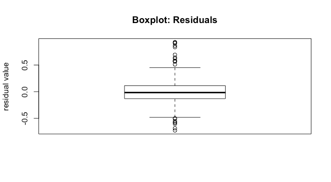
We see that the median is close to . Further, the  and
and  percentile look approximately the same distance from , and the non-outlier min and max also look about the same distance from . All of this is good as it suggests correct model specification.
Coefficients
The second thing printed by the linear regression summary call is information about the coefficients. This includes their estimates, standard errors, t statistics, and p-values.
Estimates
The intercept tells us that when all the features are at , the expected response is the intercept. Note that for an arguably better interpretation, you should consider centering your features. This changes the interpretation. Now, when features are at their mean values, the expected response is the intercept. For the other features, the estimates give us the expected change in the response due to a unit change in the feature.
Standard Error
The standard error is the standard error of our estimate, which allows us to construct marginal confidence intervals for the estimate of that particular feature. If  is the standard error and
  is the estimated coefficient for feature
  , then a 95% confidence interval is given by
  . Note that this requires two things for this confidence interval to be valid:
- your model assumptions hold
- you have enough data/samples to invoke the central limit theorem, as you need
 to be approximately Gaussian.
That is, assuming all model assumptions are satisfied, we can say that with 95% confidence (which is not probability) the true parameter  lies in
 ![[hat{beta}_i-1.96cdot s.e.(hat{beta}_i),hat{beta}_i+1.96cdot s.e.(hat{beta}_i)]](https://boostedml.com/wp-content/ql-cache/quicklatex.com-896c4923f08e9399d86b0c082a25db94_l3.png "Rendered by QuickLaTeX.com") . Based on this, we can construct confidence intervals
. Based on this, we can construct confidence intervals
confint(model)
                    2.5 %        97.5 %
(Intercept)  2.3987332457  2.8924423620
crim        -0.0111943622 -0.0056703707
rm           0.1086963289  0.1769912871
tax         -0.0004055169 -0.0001069386
lstat       -0.0334396331 -0.0256328293
Here we can see that the entire confidence interval for number of rooms has a large effect size relative to the other covariates.
t-value
The t-statistic is
(1) 
which tells us about how far our estimated parameter is from a hypothesized value, scaled by the standard deviation of the estimate. Assuming that is Gaussian, under the null hypothesis that  , this will be t distributed with
  degrees of freedom, where
  is the number of observations and
  is the number of parameters we need to estimate.
Pr(>|t|)
This is the p-value for the individual coefficient. Under the t distribution with degrees of freedom, this tells us the probability of observing a value at least as extreme as our . If this probability is sufficiently low, we can reject the null hypothesis that this coefficient is . However, note that when we care about looking at all of the coefficients, we are actually doing multiple hypothesis tests, and need to correct for that. In this case we are making five hypothesis tests, one for each feature and one for the coefficient. Instead of using the standard p-value of  , we can use the Bonferroni correction and divide by the number of hypothesis tests, and thus set our p-value threshold to
  .
.
Assessing Fit and Overall Significance
The linear regression summary printout then gives the residual standard error, the  , and the
  statistic and test. These tell us about how good a fit the model is and whether any of the coefficients are significant.
Residual Standard Error
The residual standard error is given by  . It gives the standard deviation of the residuals, and tells us about how large the prediction error is in-sample or on the training data. We’d like this to be significantly different from the variability in the marginal response distribution, otherwise it’s not clear that the model explains much.
Multiple and Adjusted 
Intuitively tells us what proportion of the variance is explained by our model, and is given by
(2) 
both and the residual standard standard deviation tells us about how well our model fits the data. The adjusted deals with an increase in spuriously due to adding features, essentially fitting noise in the data. It is given by
(3) 
thus as the number of features increases, the required needed will increase as well to maintain the same adjusted .
F-Statistic and F-test
In addition to looking at whether individual features have a significant effect, we may also wonder whether at least one feature has a significant effect. That is, we would like to test the null hypothesis
(4) 
that all coefficients are against the alternative hypothesis
(5) 
Under the null hypothesis the F statistic will be F distributed with  degrees of freedom. The probability of our observed data under the null hypothesis is then the p-value. If we use the F-test alone without looking at the t-tests, then we do not need a Bonferroni correction, while if we do look at the t-tests, we need one.
Errors are of various types and impact the research process in different ways. Here’s a deep exploration of the standard error, the types, implications, formula, and how to interpret the values
What is a Standard Error?
The standard error is a statistical measure that accounts for the extent to which a sample distribution represents the population of interest using standard deviation. You can also think of it as the standard deviation of your sample in relation to your target population.
The standard error allows you to compare two similar measures in your sample data and population. For example, the standard error of the mean measures how far the sample mean (average) of the data is likely to be from the true population mean—the same applies to other types of standard errors.
Explore: Survey Errors To Avoid: Types, Sources, Examples, Mitigation
Why is Standard Error Important?
First, the standard error of a sample accounts for statistical fluctuation.
Researchers depend on this statistical measure to know how much sampling fluctuation exists in their sample data. In other words, it shows the extent to which a statistical measure varies from sample to population.
In addition, standard error serves as a measure of accuracy. Using standard error, a researcher can estimate the efficiency and consistency of a sample to know precisely how a sampling distribution represents a population.
How Many Types of Standard Error Exist?
There are five types of standard error which are:
- Standard error of the mean
- Standard error of measurement
- Standard error of the proportion
- Standard error of estimate
- Residual Standard Error
1. Standard Error of the Mean (SEM)
The standard error of the mean accounts for the difference between the sample mean and the population mean. In other words, it quantifies how much variation is expected to be present in the sample mean that would be computed from every possible sample, of a given size, taken from the population.
How to Find SEM (With Formula)
SEM = Standard Deviation ÷ √n
Where;
n = sample size
Suppose that the standard deviation of observation is 15 with a sample size of 100. Using this formula, we can deduce the standard error of the mean as follows:
SEM = 15 ÷ √100
Standard Error of Mean in 1.5
2. Standard Error of Measurement
The standard error of measurement accounts for the consistency of scores within individual subjects in a test or examination.
This means it measures the extent to which estimated test or examination scores are spread around a true score.
A more formal way to look at it is through the 1985 lens of Aera, APA, and NCME. Here, they define a standard error as “the standard deviation of errors of measurement that is associated with the test scores for a specified group of test-takers….”
Read: 7 Types of Data Measurement Scales in Research
How to Find Standard Error of Measurement
Where;
rxx is the reliability of the test and is calculated as:
Rxx = S2T / S2X
Where;
S2T = variance of the true scores.
S2X = variance of the observed scores.
Suppose an organization has a reliability score of 0.4 and a standard deviation of 2.56. This means
SEm = 2.56 × √1–0.4 = 1.98
3. Standard Error of the Estimate
The standard error of the estimate measures the accuracy of predictions in sampling, research, and data collection. Specifically, it measures the distance that the observed values fall from the regression line which is the single line with the smallest overall distance from the line to the points.
How to Find Standard Error of the Estimate
The formula for standard error of the estimate is as follows:
Where;
σest is the standard error of the estimate;
Y is an actual score;
Y’ is a predicted score, and;
N is the number of pairs of scores.
The numerator is the sum of squared differences between the actual scores and the predicted scores.
4. Standard Error of Proportion
The standard of error of proportion in an observation is the difference between the sample proportion and the population proportion of your target audience. In more technical terms, this variable is the spread of the sample proportion about the population proportion.
How to Find Standard Error of the Proportion
The formula for calculating the standard error of the proportion is as follows:
Where;
P (hat) is equal to x ÷ n (with number of success x and the total number of observations of n)
5. Residual Standard Error
Residual standard error accounts for how well a linear regression model fits the observation in a systematic investigation. A linear regression model is simply a linear equation representing the relationship between two variables, and it helps you to predict similar variables.
How to Calculate Residual Standard Error
The formula for residual standard error is as follows:
Residual standard error = √Σ(y – ŷ)2/df
where:
y: The observed value
ŷ: The predicted value
df: The degrees of freedom, calculated as the total number of observations – total number of model parameters.
As you interpret your data, you should note that the smaller the residual standard error, the better a regression model fits a dataset, and vice versa.
How Do You Calculate Standard Error?
The formula for calculating standard error is as follows:
Where
σ – Standard deviation
n – Sample size, i.e., the number of observations in the sample
Here’s how this works in real-time.
Suppose the standard deviation of a sample is 1.5 with 4 as the sample size. This means:
Standard Error = 1.5 ÷ √4
That is; 1.5 ÷2 = 0.75
Alternatively, you can use a standard error calculator to speed up the process for larger data sets.
How to Interpret Standard Error Values
As stated earlier, researchers use the standard error to measure the reliability of observation. This means it allows you to compare how far a particular variable in the sample data is from the population of interest.
Calculating standard error is just one piece of the puzzle; you need to know how to interpret your data correctly and draw useful insights for your research. Generally, a small standard error is an indication that the sample mean is a more accurate reflection of the actual population mean, while a large standard error means the opposite.
Standard Error Example
Suppose you need to find the standard error of the mean of a data set using the following information:
Standard Deviation: 1.5
n = 13
Standard Error of the Mean = Standard Deviation ÷ √n
1.5 ÷ √13 = 0.42
How Should You Report the Standard Error?
After calculating the standard error of your observation, the next thing you should do is present this data as part of the numerous variables affecting your observation. Typically, researchers report the standard error alongside the mean or in a confidence interval to communicate the uncertainty around the mean.
Applications of Standard Error
The most common application of standard error are in statistics and economics. In statistics, standard error allows researchers to determine the confidence interval of their data sets, and in some cases, the margin of error. Researchers also use standard error in hypothesis testing and regression analysis.
FAQs About Standard Error
- What Is the Difference Between Standard Deviation and Standard Error of the Mean?
The major difference between standard deviation and standard error of the mean is how they account for the differences between the sample data and the population of interest.
Researchers use standard deviation to measure the variability or dispersion of a data set to its mean. On the other hand, the standard error of the mean accounts for the difference between the mean of the data sample and that of the target population.
Something else to note here is that the standard error of a sample is always smaller than the corresponding standard deviation.
- What Is The Symbol for Standard Error?
During calculation, the standard error is represented as σx̅.
- Is Standard Error the Same as Margin of Error?
No. Margin of Error and standard error are not the same. Researchers use the standard error to measure the preciseness of an estimate of a population, meanwhile margin of error accounts for the degree of error in results received from random sampling surveys.
The standard error is calculated as s / √n where;
s: Sample standard deviation
n: Sample size
On the other hand, margin of error = z*(s/√n) where:
z: Z value that corresponds to a given confidence level
s: Sample standard deviation
n: Sample size
Linear regression models are a key part of the family of supervised learning models.
13 mins reading time

Linear regression models are a key part of the family of supervised learning models. In particular, linear regression models are a useful tool for predicting a quantitative response. For more details, check an article I’ve written on Simple Linear Regression — An example using R. In general, statistical softwares have different ways to show a model output. This quick guide will help the analyst who is starting with linear regression in R to understand what the model output looks like.
In the example below, we’ll use the cars dataset found in the datasets package in R (for more details on the package you can call: library(help = "datasets").
##      speed           dist
##  Min.   : 4.0   Min.   :  2.00
##  1st Qu.:12.0   1st Qu.: 26.00
##  Median :15.0   Median : 36.00
##  Mean   :15.4   Mean   : 42.98
##  3rd Qu.:19.0   3rd Qu.: 56.00
##  Max.   :25.0   Max.   :120.00
The cars dataset gives Speed and Stopping Distances of Cars. This dataset is a data frame with 50 rows and 2 variables. The rows refer to cars and the variables refer to speed (the numeric Speed in mph) and dist (the numeric stopping distance in ft.). As the summary output above shows, the cars dataset’s speed variable varies from cars with speed of 4 mph to 25 mph (the data source mentions these are based on cars from the ’20s! — to find out more about the dataset, you can type ?cars). When it comes to distance to stop, there are cars that can stop in 2 feet and cars that need 120 feet to come to a stop.
Below is a scatterplot of the variables:
plot(cars, col='blue', pch=20, cex=2, main="Relationship between Speed and Stopping Distance for 50 Cars",
	xlab="Speed in mph", ylab="Stopping Distance in feet")
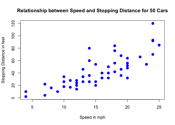
From the plot above, we can visualise that there is a somewhat strong relationship between a cars’ speed and the distance required for it to stop (i.e.: the faster the car goes the longer the distance it takes to come to a stop).
In this exercise, we will:
- Run a simple linear regression model in R and distil and interpret the key components of the R linear model output. Note that for this example we are not too concerned about actually fitting the best model but we are more interested in interpreting the model output — which would then allow us to potentially define next steps in the model building process.
Let’s get started by running one example:
set.seed(122)
speed.c = scale(cars$speed, center=TRUE, scale=FALSE)
mod1 = lm(formula = dist ~ speed.c, data = cars)
summary(mod1)
##
## Call:
## lm(formula = dist ~ speed.c, data = cars)
##
## Residuals:
##     Min      1Q  Median      3Q     Max
## -29.069  -9.525  -2.272   9.215  43.201
##
## Coefficients:
##             Estimate Std. Error t value Pr(>|t|)
## (Intercept)  42.9800     2.1750  19.761  < 2e-16 ***
## speed.c       3.9324     0.4155   9.464 1.49e-12 ***
## ---
## Signif. codes:  0 '***' 0.001 '**' 0.01 '*' 0.05 '.' 0.1 ' ' 1
##
## Residual standard error: 15.38 on 48 degrees of freedom
## Multiple R-squared:  0.6511,	Adjusted R-squared:  0.6438
## F-statistic: 89.57 on 1 and 48 DF,  p-value: 1.49e-12
The model above is achieved by using the lm() function in R and the output is called using the summary() function on the model.
Below we define and briefly explain each component of the model output:
Formula Call
As you can see, the first item shown in the output is the formula R used to fit the data. Note the simplicity in the syntax: the formula just needs the predictor (speed) and the target/response variable (dist), together with the data being used (cars).
Residuals
The next item in the model output talks about the residuals. Residuals are essentially the difference between the actual observed response values (distance to stop dist in our case) and the response values that the model predicted. The Residuals section of the model output breaks it down into 5 summary points. When assessing how well the model fit the data, you should look for a symmetrical distribution across these points on the mean value zero (0). In our example, we can see that the distribution of the residuals do not appear to be strongly symmetrical. That means that the model predicts certain points that fall far away from the actual observed points. We could take this further consider plotting the residuals to see whether this normally distributed, etc. but will skip this for this example.
Coefficients
The next section in the model output talks about the coefficients of the model. Theoretically, in simple linear regression, the coefficients are two unknown constants that represent the intercept and slope terms in the linear model. If we wanted to predict the Distance required for a car to stop given its speed, we would get a training set and produce estimates of the coefficients to then use it in the model formula. Ultimately, the analyst wants to find an intercept and a slope such that the resulting fitted line is as close as possible to the 50 data points in our data set.
Coefficient — Estimate
The coefficient Estimate contains two rows; the first one is the intercept. The intercept, in our example, is essentially the expected value of the distance required for a car to stop when we consider the average speed of all cars in the dataset. In other words, it takes an average car in our dataset 42.98 feet to come to a stop. The second row in the Coefficients is the slope, or in our example, the effect speed has in distance required for a car to stop. The slope term in our model is saying that for every 1 mph increase in the speed of a car, the required distance to stop goes up by 3.9324088 feet.
Coefficient — Standard Error
The coefficient Standard Error measures the average amount that the coefficient estimates vary from the actual average value of our response variable. We’d ideally want a lower number relative to its coefficients. In our example, we’ve previously determined that for every 1 mph increase in the speed of a car, the required distance to stop goes up by 3.9324088 feet. The Standard Error can be used to compute an estimate of the expected difference in case we ran the model again and again. In other words, we can say that the required distance for a car to stop can vary by 0.4155128 feet. The Standard Errors can also be used to compute confidence intervals and to statistically test the hypothesis of the existence of a relationship between speed and distance required to stop.
Coefficient — t value
The coefficient t-value is a measure of how many standard deviations our coefficient estimate is far away from 0. We want it to be far away from zero as this would indicate we could reject the null hypothesis — that is, we could declare a relationship between speed and distance exist. In our example, the t-statistic values are relatively far away from zero and are large relative to the standard error, which could indicate a relationship exists. In general, t-values are also used to compute p-values.
Coefficient — Pr(>t)
The Pr(>t) acronym found in the model output relates to the probability of observing any value equal or larger than t. A small p-value indicates that it is unlikely we will observe a relationship between the predictor (speed) and response (dist) variables due to chance. Typically, a p-value of 5% or less is a good cut-off point. In our model example, the p-values are very close to zero. Note the ‘signif. Codes’ associated to each estimate. Three stars (or asterisks) represent a highly significant p-value. Consequently, a small p-value for the intercept and the slope indicates that we can reject the null hypothesis which allows us to conclude that there is a relationship between speed and distance.
Residual Standard Error
Residual Standard Error is measure of the quality of a linear regression fit. Theoretically, every linear model is assumed to contain an error term E. Due to the presence of this error term, we are not capable of perfectly predicting our response variable (dist) from the predictor (speed) one. The Residual Standard Error is the average amount that the response (dist) will deviate from the true regression line. In our example, the actual distance required to stop can deviate from the true regression line by approximately 15.3795867 feet, on average. In other words, given that the mean distance for all cars to stop is 42.98 and that the Residual Standard Error is 15.3795867, we can say that the percentage error is (any prediction would still be off by) 35.78%. It’s also worth noting that the Residual Standard Error was calculated with 48 degrees of freedom. Simplistically, degrees of freedom are the number of data points that went into the estimation of the parameters used after taking into account these parameters (restriction). In our case, we had 50 data points and two parameters (intercept and slope).
Multiple R-squared, Adjusted R-squared
The R-squared ($R^2$) statistic provides a measure of how well the model is fitting the actual data. It takes the form of a proportion of variance. $R^2$ is a measure of the linear relationship between our predictor variable (speed) and our response / target variable (dist). It always lies between 0 and 1 (i.e.: a number near 0 represents a regression that does not explain the variance in the response variable well and a number close to 1 does explain the observed variance in the response variable). In our example, the $R^2$ we get is 0.6510794. Or roughly 65% of the variance found in the response variable (dist) can be explained by the predictor variable (speed). Step back and think: If you were able to choose any metric to predict distance required for a car to stop, would speed be one and would it be an important one that could help explain how distance would vary based on speed? I guess it’s easy to see that the answer would almost certainly be a yes. That why we get a relatively strong $R^2$. Nevertheless, it’s hard to define what level of $R^2$ is appropriate to claim the model fits well. Essentially, it will vary with the application and the domain studied.
A side note: In multiple regression settings, the $R^2$ will always increase as more variables are included in the model. That’s why the adjusted $R^2$ is the preferred measure as it adjusts for the number of variables considered.
F-Statistic
F-statistic is a good indicator of whether there is a relationship between our predictor and the response variables. The further the F-statistic is from 1 the better it is. However, how much larger the F-statistic needs to be depends on both the number of data points and the number of predictors. Generally, when the number of data points is large, an F-statistic that is only a little bit larger than 1 is already sufficient to reject the null hypothesis (H0 : There is no relationship between speed and distance). The reverse is true as if the number of data points is small, a large F-statistic is required to be able to ascertain that there may be a relationship between predictor and response variables. In our example the F-statistic is 89.5671065 which is relatively larger than 1 given the size of our data.
Note that the model we ran above was just an example to illustrate how a linear model output looks like in R and how we can start to interpret its components. Obviously the model is not optimised. One way we could start to improve is by transforming our response variable (try running a new model with the response variable log-transformed mod2 = lm(formula = log(dist) ~ speed.c, data = cars) or a quadratic term and observe the differences encountered). We could also consider bringing in new variables, new transformation of variables and then subsequent variable selection, and comparing between different models. Finally, with a model that is fitting nicely, we could start to run predictive analytics to try to estimate distance required for a random car to stop given its speed.