Rms error что это - Исправление ошибок и поиск оптимальных решений проблем

Содержание

Как рассчитать среднеквадратичную ошибку (RMSE) в Excel
Как рассчитать среднеквадратичную ошибку в Excel
Сценарий 1
Сценарий 2
Как интерпретировать среднеквадратичную ошибку
GIS-LAB
Среднеквадратичная ошибка (RMSE)
Ссылки по теме
Среднеквадратичная ошибка (RMSE)
Содержание
Введение
Связь со средним расстоянием
Вклад точки в общую RMSE
Допуск RMSE
Оценка RMSE

Как рассчитать среднеквадратичную ошибку (RMSE) в Excel

В статистике регрессионный анализ — это метод, который мы используем для понимания взаимосвязи между переменной-предиктором x и переменной отклика y.

Когда мы проводим регрессионный анализ, мы получаем модель, которая сообщает нам прогнозируемое значение для переменной ответа на основе значения переменной-предиктора.

Один из способов оценить, насколько «хорошо» наша модель соответствует заданному набору данных, — это вычислить среднеквадратичную ошибку , которая представляет собой показатель, который говорит нам, насколько в среднем наши прогнозируемые значения отличаются от наших наблюдаемых значений.

Формула для нахождения среднеквадратичной ошибки, чаще называемая RMSE , выглядит следующим образом:

СКО = √[ Σ(P i – O i ) 2 / n ]

Σ — причудливый символ, означающий «сумма».
P i — прогнозируемое значение для i -го наблюдения в наборе данных.
O i — наблюдаемое значение для i -го наблюдения в наборе данных.
n — размер выборки

Технические примечания:

Среднеквадратичную ошибку можно рассчитать для любого типа модели, которая дает прогнозные значения, которые затем можно сравнить с наблюдаемыми значениями набора данных.
Среднеквадратичную ошибку также иногда называют среднеквадратичным отклонением, которое часто обозначается аббревиатурой RMSD.

Далее рассмотрим пример расчета среднеквадратичной ошибки в Excel.

Как рассчитать среднеквадратичную ошибку в Excel

В Excel нет встроенной функции для расчета RMSE, но мы можем довольно легко вычислить его с помощью одной формулы. Мы покажем, как рассчитать RMSE для двух разных сценариев.

Сценарий 1

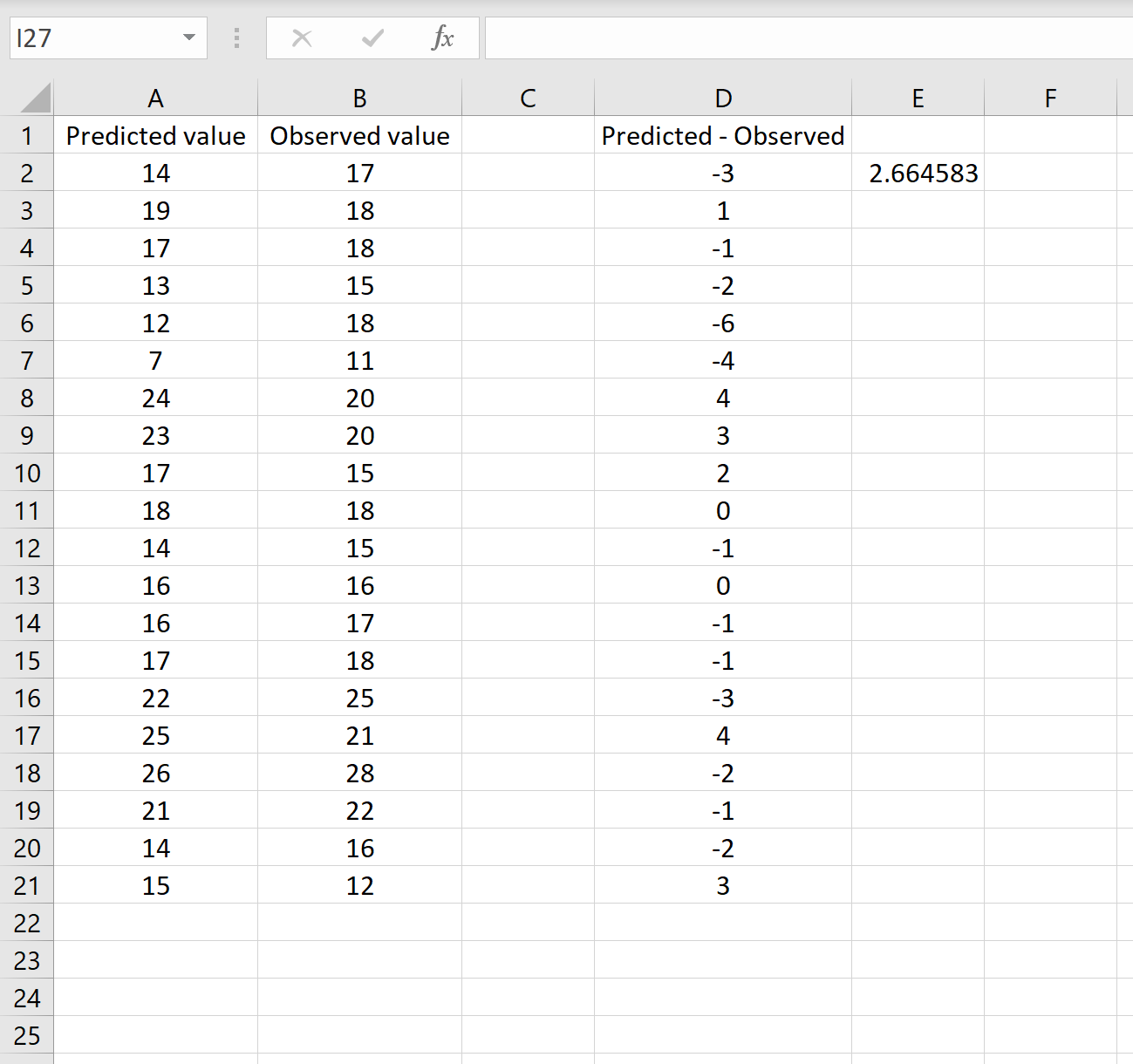
В одном сценарии у вас может быть один столбец, содержащий предсказанные значения вашей модели, и другой столбец, содержащий наблюдаемые значения. На изображении ниже показан пример такого сценария:

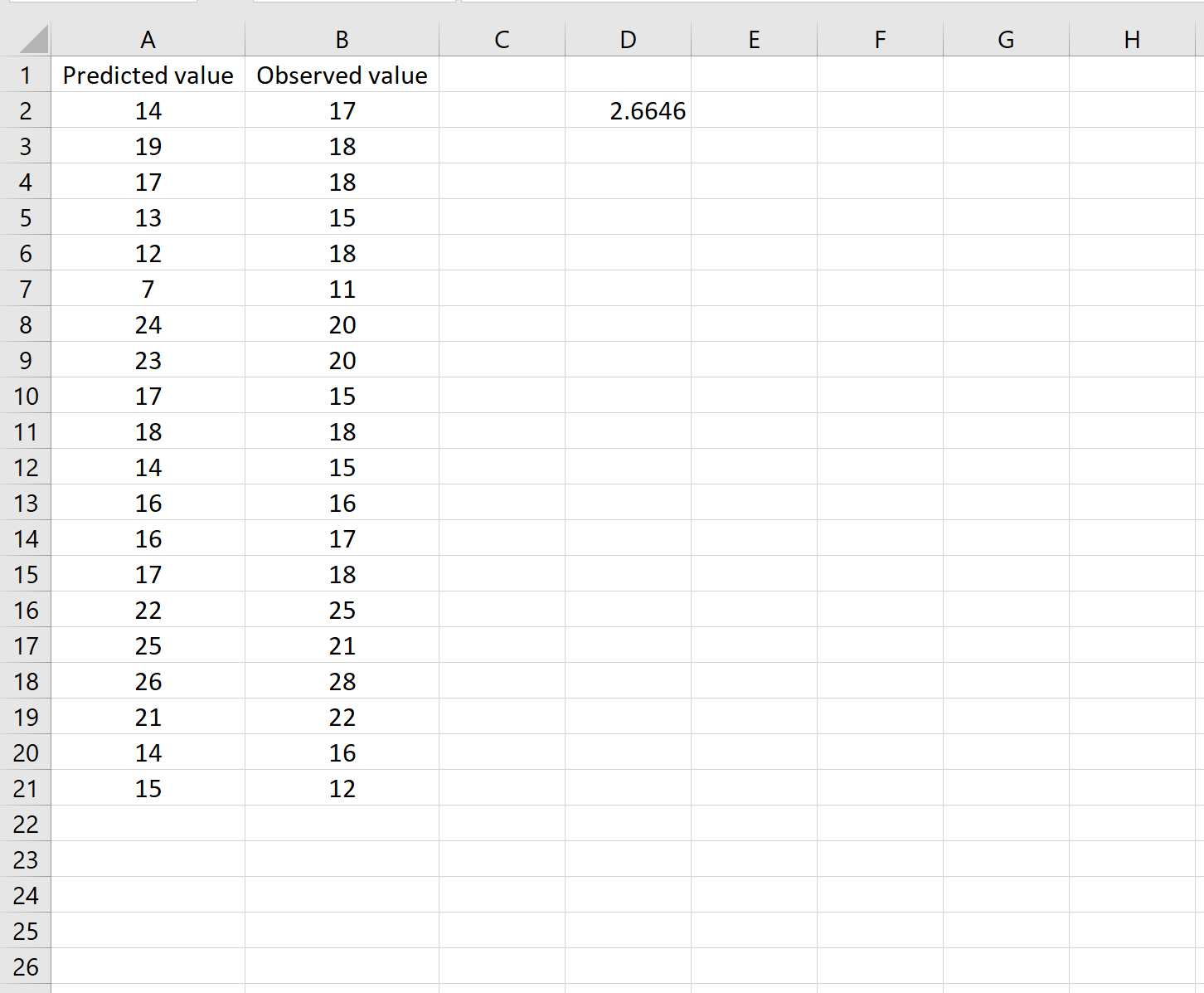
Если это так, то вы можете рассчитать RMSE, введя следующую формулу в любую ячейку, а затем нажав CTRL+SHIFT+ENTER:

=КОРЕНЬ(СУММСК(A2:A21-B2:B21) / СЧЕТЧ(A2:A21))

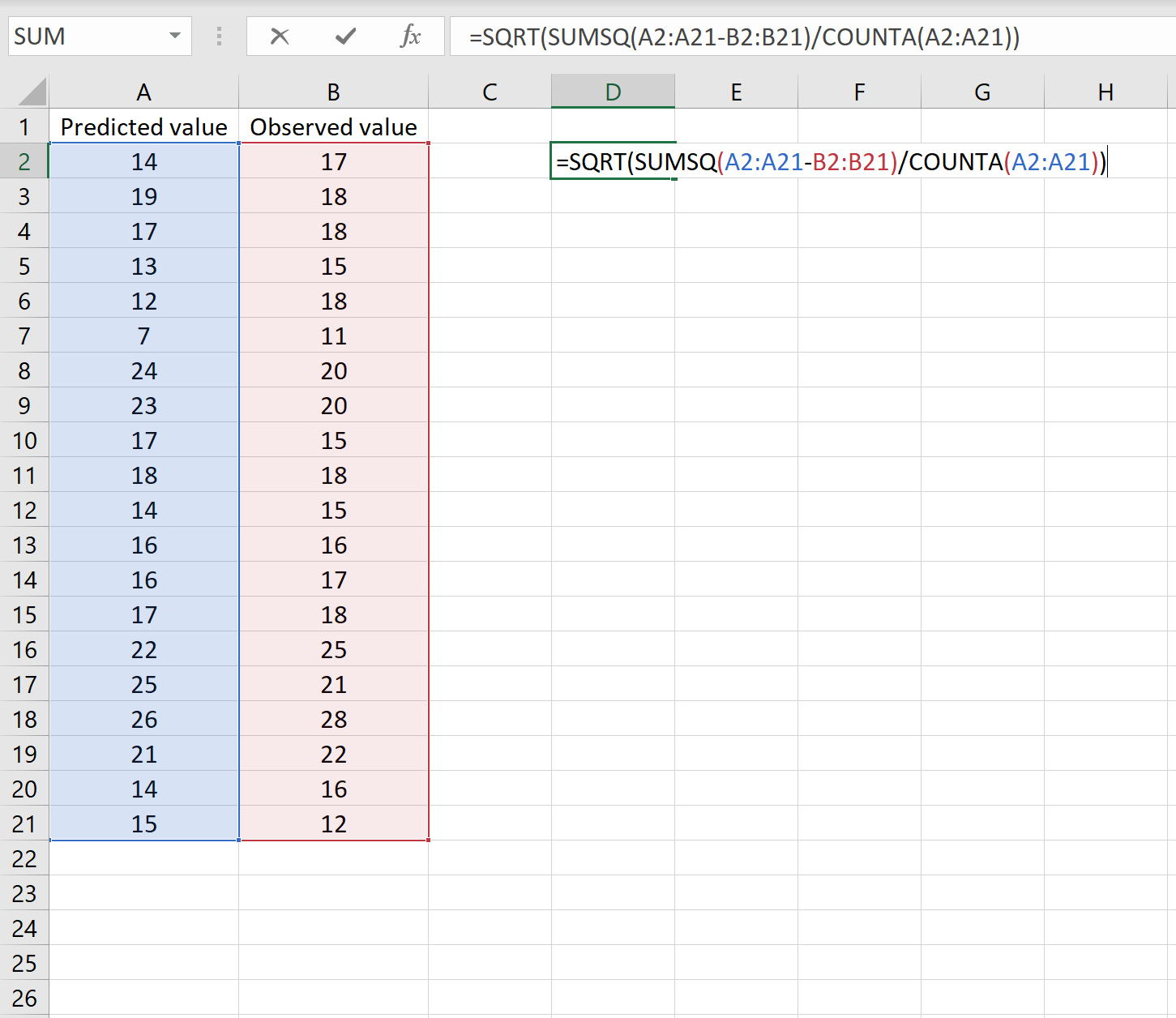
Это говорит нам о том, что среднеквадратическая ошибка равна 2,6646 .

Формула может показаться немного сложной, но она имеет смысл, если ее разобрать:

= КОРЕНЬ( СУММСК(A2:A21-B2:B21) / СЧЕТЧ(A2:A21) )

Во-первых, мы вычисляем сумму квадратов разностей между прогнозируемыми и наблюдаемыми значениями, используя функцию СУММСК() .
Затем мы делим на размер выборки набора данных, используя COUNTA() , который подсчитывает количество непустых ячеек в диапазоне.
Наконец, мы извлекаем квадратный корень из всего вычисления, используя функцию SQRT() .

Сценарий 2

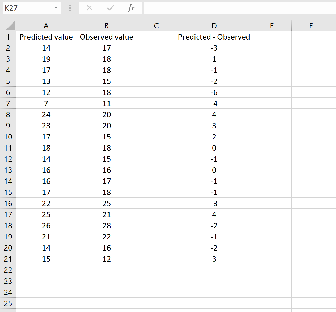
В другом сценарии вы, возможно, уже вычислили разницу между прогнозируемыми и наблюдаемыми значениями. В этом случае у вас будет только один столбец, отображающий различия.

На изображении ниже показан пример этого сценария. Прогнозируемые значения отображаются в столбце A, наблюдаемые значения — в столбце B, а разница между прогнозируемыми и наблюдаемыми значениями — в столбце D:

Если это так, то вы можете рассчитать RMSE, введя следующую формулу в любую ячейку, а затем нажав CTRL+SHIFT+ENTER:

=КОРЕНЬ(СУММСК(D2:D21) / СЧЕТЧ(D2:D21))

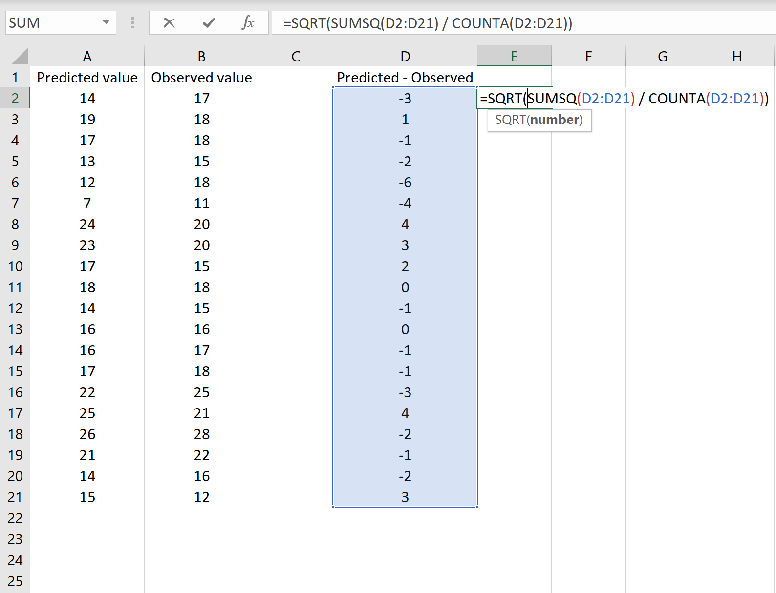
Это говорит нам о том, что среднеквадратическая ошибка равна 2,6646 , что соответствует результату, полученному в первом сценарии. Это подтверждает, что эти два подхода к расчету RMSE эквивалентны.

Формула, которую мы использовали в этом сценарии, лишь немного отличается от той, что мы использовали в предыдущем сценарии:

= КОРЕНЬ (СУММСК(D2 :D21) / СЧЕТЧ(D2:D21) )

Поскольку мы уже рассчитали разницу между предсказанными и наблюдаемыми значениями в столбце D, мы можем вычислить сумму квадратов разностей с помощью функции СУММСК().только со значениями в столбце D.
Затем мы делим на размер выборки набора данных, используя COUNTA() , который подсчитывает количество непустых ячеек в диапазоне.
Наконец, мы извлекаем квадратный корень из всего вычисления, используя функцию SQRT() .

Как интерпретировать среднеквадратичную ошибку

Как упоминалось ранее, RMSE — это полезный способ увидеть, насколько хорошо регрессионная модель (или любая модель, которая выдает прогнозируемые значения) способна «соответствовать» набору данных.

Чем больше RMSE, тем больше разница между прогнозируемыми и наблюдаемыми значениями, а это означает, что модель регрессии хуже соответствует данным. И наоборот, чем меньше RMSE, тем лучше модель соответствует данным.

Может быть особенно полезно сравнить RMSE двух разных моделей друг с другом, чтобы увидеть, какая модель лучше соответствует данным.

Для получения дополнительных руководств по Excel обязательно ознакомьтесь с нашей страницей руководств по Excel , на которой перечислены все учебные пособия Excel по статистике.

Источник

GIS-LAB

Географические информационные системы и дистанционное зондирование

Среднеквадратичная ошибка (RMSE)

Краткая объяснение что такое RMSE применительно к данным ДЗЗ

Среднеквадратичная ошибка (Root Mean Square Error, RMS Error, RMSE) — расстояние между двумя точками.

В случае если речь идет о привязке данных, в качестве точек между которыми измеряется расстояние могут выступать:

Исходная точка и конечная точки (например результат трансформации), в этом случае RMSE будет показателем насколько исходная точка близка к конечной — текущая ошибка.
Желаемое положение выходной точки (точка поставленная пользователем) и результатом ее трансформации (точка поставленная моделью). Трансформация — то или иное математическое преобразование исходных координат в конечные, примером такого преобразования может быть аффинная или полиномиальная трансформация. В данном случае RMSE показывает насколько используемая трансформация позволяет точно приблизить исходную точку к конечной, т.е. RMSE в этом случае — ошибка трансформации.

Как видно на иллюстрации ниже, выходные точки 1, 2, 3 поставленные оператором (синие) совпадают с трансформированными (расчетными) значениями (зеленые) и не видны из-за точного совпадения, а вот точка 4 поставлена не там, куда бы она попала используя ту же трансформацию, это дает возможность вычислить для нее RMSE, для точек 1, 2, 3 RMSE = 0.

Привязываемое изображение слева, изображение используемое в качестве источника координат (привязанное) справа.

Примечание: здесь и далее в статье, как и в ERDAS IMAGINE Field Guide, RMS определяется как расстояние (длина гипотенузы), что не совсем соответствует определению Root Mean Squared, так как отсутствует компонент усреднения, классический RMS должен вычисляться делением выражения под корнем на N измерений, в этом случае на 2. В данном случае удобнее называть RMS — расстоянием.

Ошибка RMS рассчитывается по следующей формуле, представляющей из себя формулу вычисления расстояния:

где x_i, y_i — исходные координаты, x_r, y_r — конечные координаты

RMSE выражается как расстояние в единицах исходной системы координат, то есть, если вы привязываете только что отсканированную карту, то RMSE будет выражаться в пикселях (или долях пикселя), если вы производите дополнительную привязку снимка, то RMSE будет показывать значения в метрах. Значение RMSE равное 2 для определенной точки будет означать, что ее исходная координата удалена на 2 пикселя или метра от конечной (расчетной) точки.

Чтобы лучше понять когда и как можно получить RMSE при привязке можно использовать следующий алгоритм, иллюстрирующую процесс привязки с помощью аффинного преобразования:

Получение изображения, например сканированием, изображение получает пиксельную систему координат X,Y (колонка, ряд).
Расстановка трех точек с начальными и конечными координатами. Эти координаты указывают:
- Начальные координаты — положение точки на непривязанном материале (координаты конкретного пиксела по системе ряд/колонка);
- Конечные координаты — положение точки на привязанном материале, любом источнике координат, географических или спроектированных.
Три точки — минимальное количество, необходимое для того, чтобы решить систему уравнений аффинного преобразования:

Решение уравнения заключается в нахождении всех шести коэффициентов, например решением системы уравнений:

x1′ = a + b*x1 + c*y1
y1′ = d + e*x1 + f*y1
x2′ = a + b*x2 + c*y2
y2′ = d + e*x2 + f*y2
x3′ = a + b*x3 + c*y3
y3′ = d + e*x3 + f*y3

Если точек меньше чем минимально необходимо — решить систему невозможно, нельзя найти коэффициенты трансформации и соответственно невозможно произвести пересчет координат. RMSE для точек также вычислить невозможно.

Расстановка минимально необходимого количества точек для данного преобразования (трех) приводит к тому, что RMSE для каждой точки становится равна 0. Можно производить трансформацию. Однако в таком случае мы не можем сделать выводов о качестве точек, ведь для этого надо рассчитать RMSE, а значит.

Ставим дополнительные точки. Появление новых данных как правило приводит к тому, что то положение, куда мы ставим конечную точку в процессе привязки и ее расчетное положение не совпадают. Это делает возможным расчет RMS ошибки.

С примером и математикой расчета полиномиального преобразования 2-ой степени можно прочитать в статье «Полиномиальные преобразования — вычисления и практика».

Помимо RMSE часто также можно увидеть также значения ошибки по одной из осей X или Y. Эти значения являются остатками (residuals) и могут быть рассчитаны для каждой точки. Изучение значений этих ошибок может помочь понять, почему привязанный материал смещен по одной из осей. Это проблема часто возникает при привязке данных полученных при съемке под углом (не в надир).

Уравнение вычисления RMS для каждой точки можно переписать как:

где XR и YR — остаточные ошибки по X и Y соответственно.

Графически ошибки по X и Y, а также RMSE соотносятся следующим образом:

Вычислив RMSE для каждой точки, можно также определить общую ошибку по X (Rx), Y (Ry) и общую RMSE (T) используя следующие формулы:

где n — число контрольных точек, i — порядковый номер контрольной точки, d — расстояние между парой точек.

Связь со средним расстоянием

Другим, достаточно объективным, способом оценить точность привязки является среднее расстояние, которое очень похоже по формуле на RMSE, но является менее консервативным показателем, так как расстояния не возводятся в квадрат как в RMSE. Выразив расстояние через d, приведем для сравнения формулы вычисления общей RMSE (T) и среднего расстояния (MD):

RMSE является более общеупотребимым в литературе.

Другим распространенным способом описания точности набора измерений являются квантили дробные стандартному отклонению (сигма).

Вклад точки в общую RMSE

Для того, чтобы вычислить вклад точки в общую ошибку (E_i), необходимо разделить RMSE этой точки (R_i) на общую RMSE.

Допуск RMSE

В большинстве случаев, вместо того, чтобы усложнять тип трансформации (например переходить к более высоким порядкам полиномиальных преобразований) имеет смысл допустить некоторую ошибку. Величину допустимой RMSE можно представить как окно, окружающее точку с желаемыми координатами, положением расчетной точки внутри которого считается корректным. Например, если допуск RMSE равен 2, то расчетный пиксел может находится в двух пикселях от указанного оператором и являться допустимым. Величина допустимой ошибки зависит от типа и точности данных, задачи и точности контрольных точек.

Важно помнить, что RMSE указывается в пикселях, поэтому, если привязываются данные Landsat имеющие разрешение 30 метров и задача осуществить привязку с точностью не меньше тех же 30 метров, то RMSE не должна превышать 1.00 (пикселя).

Оценка RMSE

Если RMSE расчитана и найдена слишком высокой, есть 4 варианта решения проблемы:

Найти и удалить контрольные точки с большой RMSE, подразумевая, что это наименее точные точки. Это чревато еще возникновением еще больших ошибок, если отбраковываемая точка — единственная на большой участок изображения.
Увеличить допуск RMSE.
Увеличить сложность функции трансформации, которая более точно будет соответствовать введенным точкам. RMSE точек при этом уменьшится, однако использование сложных криволинейных функций может привести к нежелательным сильным искажениям растра.
Оставить только точки в которых Вы уверены, что они правильны.

В статье использованы материалы ERDAS IMAGINE Field Guide

Ссылки по теме

Последнее обновление: September 09 2021

Дата создания: 27.07.2007
Автор(ы): Максим Дубинин

Источник

Среднеквадратичная ошибка (RMSE)

Краткая объяснение что такое RMSE применительно к данным ДЗЗ

Содержание

Введение

Среднеквадратичная ошибка (Root Mean Square Error, RMS Error, RMSE) — расстояние между двумя точками.

Исходная точка и конечная точки (например результат трансформации), в этом случае RMSE будет показателем насколько исходная точка близка к конечной — текущая ошибка.
Желаемое положение выходной точки (точка поставленная пользователем) и результатом ее трансформации (точка поставленная моделью). Трансформация — то или иное математическое преобразование исходных координат в конечные, примером такого преобразования может быть аффинная или полиномиальная трансформация. В данном случае RMSE показывает насколько используемая трансформация позволяет точно приблизить исходную точку к конечной, т.е. RMSE в этом случае — ошибка трансформации.

Ошибка RMS рассчитывается по следующей формуле, представляющей из себя формулу вычисления расстояния:

где x_i, y_i — исходные координаты, x_r, y_r — конечные координаты

Получение изображения, например сканированием, изображение получает пиксельную систему координат X,Y (колонка, ряд).
Расстановка трех точек с начальными и конечными координатами. Эти координаты указывают:
- Начальные координаты — положение точки на непривязанном материале (координаты конкретного пиксела по системе ряд/колонка);
- Конечные координаты — положение точки на привязанном материале, любом источнике координат, географических или спроектированных.
Три точки — минимальное количество, необходимое для того, чтобы решить систему уравнений аффинного преобразования:
x = a+ b* x + c*y
y = d + e*x + f*y Решение уравнения заключается в нахождении всех шести коэффициентов, например решением системы уравнений:
x1′ = a + b*x1 + c*y1
y1′ = d + e*x1 + f*y1
x2′ = a + b*x2 + c*y2
y2′ = d + e*x2 + f*y2
x3′ = a + b*x3 + c*y3
y3′ = d + e*x3 + f*y3 Если точек меньше чем минимально необходимо — решить систему невозможно, нельзя найти коэффициенты трансформации и соответственно невозможно произвести пересчет координат. RMSE для точек также вычислить невозможно.
Расстановка минимально необходимого количества точек для данного преобразования (трех) приводит к тому, что RMSE для каждой точки становится равна 0. Можно производить трансформацию. Однако в таком случае мы не можем сделать выводов о качестве точек, ведь для этого надо рассчитать RMSE, а значит.
Ставим дополнительные точки. Появление новых данных как правило приводит к тому, что то положение, куда мы ставим конечную точку в процессе привязки и ее расчетное положение не совпадают. Это делает возможным расчет RMS ошибки.

Уравнение вычисления RMS для каждой точки можно переписать как:

где XR и YR — остаточные ошибки по X и Y соответственно.

Графически ошибки по X и Y, а также RMSE соотносятся следующим образом:

где n — число контрольных точек, i — порядковый номер контрольной точки, d — расстояние между парой точек.

Связь со средним расстоянием

RMSE является более общеупотребимым в литературе.

Вклад точки в общую RMSE

Для того, чтобы вычислить вклад точки в общую ошибку (E_i), необходимо разделить RMSE этой точки (R_i) на общую RMSE.

Допуск RMSE

Оценка RMSE

Если RMSE расчитана и найдена слишком высокой, есть 4 варианта решения проблемы:

Найти и удалить контрольные точки с большой RMSE, подразумевая, что это наименее точные точки. Это чревато еще возникновением еще больших ошибок, если отбраковываемая точка — единственная на большой участок изображения.
Увеличить допуск RMSE.
Увеличить сложность функции трансформации, которая более точно будет соответствовать введенным точкам. RMSE точек при этом уменьшится, однако использование сложных криволинейных функций может привести к нежелательным сильным искажениям растра.
Оставить только точки в которых Вы уверены, что они правильны.

В статье использованы материалы ERDAS IMAGINE Field Guide

Источник

From Wikipedia, the free encyclopedia

The root-mean-square deviation (RMSD) or root-mean-square error (RMSE) is a frequently used measure of the differences between values (sample or population values) predicted by a model or an estimator and the values observed. The RMSD represents the square root of the second sample moment of the differences between predicted values and observed values or the quadratic mean of these differences. These deviations are called residuals when the calculations are performed over the data sample that was used for estimation and are called errors (or prediction errors) when computed out-of-sample. The RMSD serves to aggregate the magnitudes of the errors in predictions for various data points into a single measure of predictive power. RMSD is a measure of accuracy, to compare forecasting errors of different models for a particular dataset and not between datasets, as it is scale-dependent.^[1]

RMSD is always non-negative, and a value of 0 (almost never achieved in practice) would indicate a perfect fit to the data. In general, a lower RMSD is better than a higher one. However, comparisons across different types of data would be invalid because the measure is dependent on the scale of the numbers used.

RMSD is the square root of the average of squared errors. The effect of each error on RMSD is proportional to the size of the squared error; thus larger errors have a disproportionately large effect on RMSD. Consequently, RMSD is sensitive to outliers.^[2]^[3]

Formula[edit]

The RMSD of an estimator with respect to an estimated parameter theta is defined as the square root of the mean squared error:

$operatorname{RMSD}(hat{theta}) = sqrt{operatorname{MSE}(hat{theta})} = sqrt{operatorname{E}((hat{theta}-theta)^2)}.$

For an unbiased estimator, the RMSD is the square root of the variance, known as the standard deviation.

The RMSD of predicted values hat y_t for times t of a regression’s dependent variable ${displaystyle y_{t},}$ with variables observed over T times, is computed for T different predictions as the square root of the mean of the squares of the deviations:

${displaystyle operatorname {RMSD} ={sqrt {frac {sum _{t=1}^{T}({hat {y}}_{t}-y_{t})^{2}}{T}}}.}$

(For regressions on cross-sectional data, the subscript t is replaced by i and T is replaced by n.)

In some disciplines, the RMSD is used to compare differences between two things that may vary, neither of which is accepted as the «standard». For example, when measuring the average difference between two time series $x_{1,t}$ and $x_{2,t}$ ,
the formula becomes

${displaystyle operatorname {RMSD} ={sqrt {frac {sum _{t=1}^{T}(x_{1,t}-x_{2,t})^{2}}{T}}}.}$

Normalization[edit]

Normalizing the RMSD facilitates the comparison between datasets or models with different scales. Though there is no consistent means of normalization in the literature, common choices are the mean or the range (defined as the maximum value minus the minimum value) of the measured data:^[4]

$mathrm{NRMSD} = frac{mathrm{RMSD}}{y_max -y_min}$

or ${displaystyle mathrm {NRMSD} ={frac {mathrm {RMSD} }{bar {y}}}}$

This value is commonly referred to as the normalized root-mean-square deviation or error (NRMSD or NRMSE), and often expressed as a percentage, where lower values indicate less residual variance. In many cases, especially for smaller samples, the sample range is likely to be affected by the size of sample which would hamper comparisons.

Another possible method to make the RMSD a more useful comparison measure is to divide the RMSD by the interquartile range. When dividing the RMSD with the IQR the normalized value gets less sensitive for extreme values in the target variable.

${displaystyle mathrm {RMSDIQR} ={frac {mathrm {RMSD} }{IQR}}}$

where ${displaystyle IQR=Q_{3}-Q_{1}}$

with ${displaystyle Q_{1}={text{CDF}}^{-1}(0.25)}$ and $Q_3 = text{CDF}^{-1}(0.75) ,$ where CDF⁻¹ is the quantile function.

When normalizing by the mean value of the measurements, the term coefficient of variation of the RMSD, CV(RMSD) may be used to avoid ambiguity.^[5] This is analogous to the coefficient of variation with the RMSD taking the place of the standard deviation.

${displaystyle mathrm {CV(RMSD)} ={frac {mathrm {RMSD} }{bar {y}}}.}$

Mean absolute error[edit]

Some researchers have recommended the use of the Mean Absolute Error (MAE) instead of the Root Mean Square Deviation. MAE possesses advantages in interpretability over RMSD. MAE is the average of the absolute values of the errors. MAE is fundamentally easier to understand than the square root of the average of squared errors. Furthermore, each error influences MAE in direct proportion to the absolute value of the error, which is not the case for RMSD.^[2] However, MAE is not a substitute, as it accounts only for the systematic errors, while RMSD accounts for both systematic and random errors^{[according to whom?]}.

Applications[edit]

In meteorology, to see how effectively a mathematical model predicts the behavior of the atmosphere.
In bioinformatics, the root-mean-square deviation of atomic positions is the measure of the average distance between the atoms of superimposed proteins.
In structure based drug design, the RMSD is a measure of the difference between a crystal conformation of the ligand conformation and a docking prediction.
In economics, the RMSD is used to determine whether an economic model fits economic indicators. Some experts have argued that RMSD is less reliable than Relative Absolute Error.^[6]
In experimental psychology, the RMSD is used to assess how well mathematical or computational models of behavior explain the empirically observed behavior.
In GIS, the RMSD is one measure used to assess the accuracy of spatial analysis and remote sensing.
In hydrogeology, RMSD and NRMSD are used to evaluate the calibration of a groundwater model.^[7]
In imaging science, the RMSD is part of the peak signal-to-noise ratio, a measure used to assess how well a method to reconstruct an image performs relative to the original image.
In computational neuroscience, the RMSD is used to assess how well a system learns a given model.^[8]
In protein nuclear magnetic resonance spectroscopy, the RMSD is used as a measure to estimate the quality of the obtained bundle of structures.
Submissions for the Netflix Prize were judged using the RMSD from the test dataset’s undisclosed «true» values.
In the simulation of energy consumption of buildings, the RMSE and CV(RMSE) are used to calibrate models to measured building performance.^[9]
In X-ray crystallography, RMSD (and RMSZ) is used to measure the deviation of the molecular internal coordinates deviate from the restraints library values.
In control theory, the RMSE is used as a quality measure to evaluate the performance of a State observer.^[10]

References[edit]

^ Hyndman, Rob J.; Koehler, Anne B. (2006). «Another look at measures of forecast accuracy». International Journal of Forecasting. 22 (4): 679–688. CiteSeerX 10.1.1.154.9771. doi:10.1016/j.ijforecast.2006.03.001.
^ ^a ^b Pontius, Robert; Thontteh, Olufunmilayo; Chen, Hao (2008). «Components of information for multiple resolution comparison between maps that share a real variable». Environmental Ecological Statistics. 15 (2): 111–142. doi:10.1007/s10651-007-0043-y.
^ Willmott, Cort; Matsuura, Kenji (2006). «On the use of dimensioned measures of error to evaluate the performance of spatial interpolators». International Journal of Geographical Information Science. 20: 89–102. doi:10.1080/13658810500286976.
^ «Coastal Inlets Research Program (CIRP) Wiki — Statistics». Retrieved 4 February 2015.
^ «FAQ: What is the coefficient of variation?». Retrieved 19 February 2019.
^ Armstrong, J. Scott; Collopy, Fred (1992). «Error Measures For Generalizing About Forecasting Methods: Empirical Comparisons» (PDF). International Journal of Forecasting. 8 (1): 69–80. CiteSeerX 10.1.1.423.508. doi:10.1016/0169-2070(92)90008-w.
^ Anderson, M.P.; Woessner, W.W. (1992). Applied Groundwater Modeling: Simulation of Flow and Advective Transport (2nd ed.). Academic Press.
^ Ensemble Neural Network Model
^ ANSI/BPI-2400-S-2012: Standard Practice for Standardized Qualification of Whole-House Energy Savings Predictions by Calibration to Energy Use History
^ https://kalman-filter.com/root-mean-square-error

Источник

17 авг. 2022 г.
читать 3 мин

Формула для нахождения среднеквадратичной ошибки, чаще называемая RMSE , выглядит следующим образом:

СКО = √[ Σ(P i – O i ) 2 / n ]

куда:

Σ — причудливый символ, означающий «сумма».
P i — прогнозируемое значение для i -го наблюдения в наборе данных.
O i — наблюдаемое значение для i -го наблюдения в наборе данных.
n — размер выборки

Технические примечания:

Среднеквадратичную ошибку можно рассчитать для любого типа модели, которая дает прогнозные значения, которые затем можно сравнить с наблюдаемыми значениями набора данных.
Среднеквадратичную ошибку также иногда называют среднеквадратичным отклонением, которое часто обозначается аббревиатурой RMSD.

Далее рассмотрим пример расчета среднеквадратичной ошибки в Excel.

Как рассчитать среднеквадратичную ошибку в Excel

Сценарий 1

Если это так, то вы можете рассчитать RMSE, введя следующую формулу в любую ячейку, а затем нажав CTRL+SHIFT+ENTER:

=КОРЕНЬ(СУММСК(A2:A21-B2:B21) / СЧЕТЧ(A2:A21))

Это говорит нам о том, что среднеквадратическая ошибка равна 2,6646 .

Формула может показаться немного сложной, но она имеет смысл, если ее разобрать:

= КОРЕНЬ( СУММСК(A2:A21-B2:B21) / СЧЕТЧ(A2:A21) )

Во-первых, мы вычисляем сумму квадратов разностей между прогнозируемыми и наблюдаемыми значениями, используя функцию СУММСК() .
Затем мы делим на размер выборки набора данных, используя COUNTA() , который подсчитывает количество непустых ячеек в диапазоне.
Наконец, мы извлекаем квадратный корень из всего вычисления, используя функцию SQRT() .

Сценарий 2

Если это так, то вы можете рассчитать RMSE, введя следующую формулу в любую ячейку, а затем нажав CTRL+SHIFT+ENTER:

=КОРЕНЬ(СУММСК(D2:D21) / СЧЕТЧ(D2:D21))

= КОРЕНЬ (СУММСК(D2 :D21) / СЧЕТЧ(D2:D21) )

Поскольку мы уже рассчитали разницу между предсказанными и наблюдаемыми значениями в столбце D, мы можем вычислить сумму квадратов разностей с помощью функции СУММСК().только со значениями в столбце D.
Затем мы делим на размер выборки набора данных, используя COUNTA() , который подсчитывает количество непустых ячеек в диапазоне.
Наконец, мы извлекаем квадратный корень из всего вычисления, используя функцию SQRT() .

Как интерпретировать среднеквадратичную ошибку

Источник

Regression analysis is a technique we can use to understand the relationship between one or more predictor variables and a response variable.

One way to assess how well a regression model fits a dataset is to calculate the root mean square error, which is a metric that tells us the average distance between the predicted values from the model and the actual values in the dataset.

The lower the RMSE, the better a given model is able to “fit” a dataset.

The formula to find the root mean square error, often abbreviated RMSE, is as follows:

RMSE = √Σ(P_i – O_i)² / n

where:

Σ is a fancy symbol that means “sum”
P_i is the predicted value for the i^th observation in the dataset
O_i is the observed value for the i^th observation in the dataset
n is the sample size

The following example shows how to interpret RMSE for a given regression model.

Example: How to Interpret RMSE for a Regression Model

Suppose we would like to build a regression model that uses “hours studied” to predictor “exam score” of students on a particular college entrance exam.

We collect the following data for 15 students:

We then use statistical software (like Excel, SPSS, R, Python) etc. to find the following fitted regression model:

Exam Score = 75.95 + 3.08*(Hours Studied)

We can then use this equation to predict the exam score of each student, based on how many hours they studied:

We can then calculate the squared difference between each predicted exam score and the actual exam score. Then we can take the square root of the mean of these differences:

The RMSE for this regression model turns out to be 5.681.

Recall that the residuals of a regression model are the differences between the observed data values and the predicted values from the model.

Residual = (P_i – O_i)

where

P_i is the predicted value for the i^th observation in the dataset
O_i is the observed value for the i^th observation in the dataset

And recall that the RMSE of a regression model is calculated as:

RMSE = √Σ(P_i – O_i)² / n

This means that the RMSE represents the square root of the variance of the residuals.

This is a useful value to know because it gives us an idea of the average distance between the observed data values and the predicted data values.

This is in contrast to the R-squared of the model, which tells us the proportion of the variance in the response variable that can be explained by the predictor variable(s) in the model.

Comparing RMSE Values from Different Models

The RMSE is particularly useful for comparing the fit of different regression models.

For example, suppose we want to build a regression model to predict the exam score of students and we want to find the best possible model among several potential models.

Suppose we fit three different regression models and find their corresponding RMSE values:

RMSE of Model 1: 14.5
RMSE of Model 2: 16.7
RMSE of Model 3: 9.8

Model 3 has the lowest RMSE, which tells us that it’s able to fit the dataset the best out of the three potential models.

Additional Resources

RMSE Calculator
How to Calculate RMSE in Excel
How to Calculate RMSE in R
How to Calculate RMSE in Python

Источник

$begingroup$

What is the significance of the square root in root-mean-square-error? Essentially, my question is: what is the difference between (rms error) and (rms error)$^2$?

Ethan

1,5808 gold badges20 silver badges38 bronze badges

asked Jun 29, 2015 at 13:09

$endgroup$

$begingroup$

It depends on what you are using the RMSE for. If you are merely trying to compare two models/estimators, then there is no significance to the square root. However, if you are trying to plot the error in terms of the same units as you made the measurements/estimates, then you need to take the square root to transform the squared units to the original units (much like variance vs standard deviation)

answered Jun 29, 2015 at 16:32

$endgroup$

$begingroup$

The square in RMSE is used because it always gives a positive value for error, so avoiding errors cancelling each other out, and affords greater weight to values further from the target function, so emphasising points for which the estimator is poor.

The square root is used to remove the effects of the squaring.

You could look at using the Mean Absolute Error ( MAE ) which does not have the distance weighting effect of the RMSE and just takes the average of the absolute value of the errors.

answered Jun 30, 2015 at 10:52

$endgroup$

$begingroup$

If the set that you are using the RMSE on is a linear space, a good reason to use the square root is that you turn the set into a metric space. The square root ensures the right scaling property. Essentially, the RMSE is equivalent to the Euclidean norm. As a benefit, it is possible to use results of the general theory of metric spaces.

answered Jul 3, 2015 at 5:38

$endgroup$

Источник

$begingroup$

What is the significance of the square root in root-mean-square-error? Essentially, my question is: what is the difference between (rms error) and (rms error)$^2$?

Ethan

1,5808 gold badges20 silver badges38 bronze badges

asked Jun 29, 2015 at 13:09

$endgroup$

$begingroup$

answered Jun 29, 2015 at 16:32

$endgroup$

$begingroup$

The square root is used to remove the effects of the squaring.

You could look at using the Mean Absolute Error ( MAE ) which does not have the distance weighting effect of the RMSE and just takes the average of the absolute value of the errors.

answered Jun 30, 2015 at 10:52

$endgroup$

$begingroup$

answered Jul 3, 2015 at 5:38

$endgroup$

Источник

Среднеквадратичное отклонение

Из Википедии, бесплатной энциклопедии

Перейти к навигации
Перейти к поиску

Среднеквадратичное отклонение ( RMSD ) или среднеквадратическая ошибка ( RMSE ) — часто используемая мера различий между значениями (выборочными или популяционными), предсказанными моделью или оценщиком , и наблюдаемыми значениями. RMSD представляет собой квадратный корень из второго момента выборки различий между предсказанными значениями и наблюдаемыми значениями или среднеквадратичное значение этих различий. Эти отклонения называются остатками , когда расчеты выполняются по выборке данных, которая использовалась для оценки, и называются ошибками .(или ошибки предсказания) при вычислении вне выборки. RMSD служит для объединения величин ошибок в прогнозах для различных точек данных в единую меру прогностической способности. RMSD — это мера точности для сравнения ошибок прогнозирования различных моделей для определенного набора данных, а не между наборами данных, поскольку он зависит от масштаба. ^[1]

RMSD всегда неотрицательно, и значение 0 (почти никогда не достигаемое на практике) указывает на идеальное соответствие данным. Как правило, более низкое RMSD лучше, чем более высокое. Однако сравнения различных типов данных были бы недействительными, поскольку мера зависит от масштаба используемых чисел.

RMSD — это квадратный корень из среднего квадрата ошибок. Влияние каждой ошибки на RMSD пропорционально величине квадрата ошибки; таким образом, большие ошибки оказывают непропорционально большое влияние на RMSD. Следовательно, RMSD чувствителен к выбросам. ^[2]^[3]

Формула

RMSD оценщика по расчетному параметруопределяется как квадратный корень из среднеквадратичной ошибки :

Для несмещенной оценки RMSD представляет собой квадратный корень из дисперсии , известной как стандартное отклонение .

СКО прогнозируемых значенийдля времен t зависимой переменной регрессии с переменными, наблюдаемыми в течение T раз, вычисляется для T различных прогнозов как квадратный корень из среднего значения квадратов отклонений:

(Для регрессий по данным поперечного сечения нижний индекс t заменяется на i , а T заменяется на n .)

В некоторых дисциплинах RMSD используется для сравнения различий между двумя вещами, которые могут различаться, ни одна из которых не принята в качестве «стандарта». Например, при измерении средней разницы между двумя временными рядамиа также, формула становится

Нормализация

Нормализация RMSD облегчает сравнение наборов данных или моделей с разными масштабами. Хотя в литературе нет последовательных способов нормализации, обычно выбирают среднее значение или диапазон (определяемый как максимальное значение минус минимальное значение) измеренных данных: ^[4]

или же.

Это значение обычно называют нормализованным среднеквадратичным отклонением или ошибкой (NRMSD или NRMSE) и часто выражают в процентах, где более низкие значения указывают на меньшую остаточную дисперсию. Во многих случаях, особенно для небольших выборок, диапазон выборки, вероятно, будет зависеть от размера выборки, что затруднит сравнение.

Другой возможный способ сделать среднеквадратичное отклонение более полезной мерой сравнения — разделить среднеквадратичное отклонение на межквартильный размах . При делении RMSD на IQR нормализованное значение становится менее чувствительным к экстремальным значениям целевой переменной.

куда

са такжегде CDF ⁻¹ — функция квантиля .

При нормировании по среднему значению измерений можно использовать термин коэффициент вариации СКО, CV(RMSD) , чтобы избежать неоднозначности. ^[5] Это аналогично коэффициенту вариации , где вместо стандартного отклонения используется среднеквадратичное отклонение .

Средняя абсолютная ошибка

Некоторые исследователи рекомендуют использовать среднюю абсолютную ошибку (MAE) вместо среднеквадратичного отклонения. MAE обладает преимуществами в интерпретируемости по сравнению с RMSD. MAE – это среднее абсолютных значений ошибок. MAE принципиально легче понять, чем квадратный корень из среднего квадрата ошибок. Кроме того, каждая ошибка влияет на MAE прямо пропорционально абсолютному значению ошибки, чего нельзя сказать о RMSD. ^[2]

Приложения

В метеорологии , чтобы увидеть, насколько эффективно математическая модель предсказывает поведение атмосферы .
В биоинформатике среднеквадратичное отклонение положений атомов является мерой среднего расстояния между атомами наложенных друг на друга белков .
В дизайне лекарств на основе структуры RMSD является мерой различия между кристаллической конформацией конформации лиганда и предсказанием стыковки .
В экономике RMSD используется для определения того, соответствует ли экономическая модель экономическим показателям . Некоторые эксперты утверждают, что RMSD менее надежен, чем относительная абсолютная ошибка. ^[6]
В экспериментальной психологии RMSD используется для оценки того, насколько хорошо математические или вычислительные модели поведения объясняют эмпирически наблюдаемое поведение.
В ГИС среднеквадратичное отклонение является одним из показателей, используемых для оценки точности пространственного анализа и дистанционного зондирования.
В гидрогеологии RMSD и NRMSD используются для оценки калибровки модели подземных вод. ^[7]
В области обработки изображений среднеквадратичное отклонение является частью пикового отношения сигнал/шум — меры, используемой для оценки того, насколько хорошо метод восстановления изображения работает по сравнению с исходным изображением.
В вычислительной нейробиологии RMSD используется для оценки того, насколько хорошо система изучает данную модель. ^[8]
В спектроскопии ядерного магнитного резонанса белков RMSD используется в качестве меры для оценки качества полученного набора структур.
Заявки на получение премии Netflix оценивались с использованием RMSD из нераскрытых «истинных» значений набора тестовых данных.
При моделировании энергопотребления зданий RMSE и CV(RMSE) используются для калибровки моделей в соответствии с измеренными характеристиками здания . ^[9]
В рентгеновской кристаллографии RMSD (и RMSZ) используется для измерения отклонения внутренних координат молекул от значений библиотеки ограничений.

Смотрите также

Среднеквадратичное значение
Средняя абсолютная ошибка
Среднее абсолютное отклонение
Среднее отклонение со знаком
Среднеквадратичное отклонение
Квадратные отклонения
Ошибки и невязки в статистике

Ссылки

^ Гайндман, Роб Дж .; Келер, Энн Б. (2006). «Еще один взгляд на показатели точности прогнозов». Международный журнал прогнозирования . 22 (4): 679–688. CiteSeerX 10.1.1.154.9771 . doi : 10.1016/j.ijforecast.2006.03.001 .
^ ^б Понтий, Роберт ^;Тонте, Олуфунмилайо; Чен, Хао (2008). «Компоненты информации для сравнения нескольких разрешений между картами, которые имеют общую реальную переменную». Экологическая экологическая статистика . 15 (2): 111–142. doi : 10.1007/s10651-007-0043-y .
^ Уиллмотт, Корт; Мацуура, Кендзи (2006). «Об использовании размерных мер ошибки для оценки производительности пространственных интерполяторов». Международный журнал географической информатики . 20 : 89–102. дои : 10.1080/13658810500286976 .
^ «Вики-программа исследования прибрежных бухт (CIRP) — Статистика» . Проверено 4 февраля 2015 г.
^ «Часто задаваемые вопросы: что такое коэффициент вариации?» . Проверено 19 февраля 2019 г.
^ Армстронг, Дж. Скотт; Коллопи, Фред (1992). «Меры погрешности для обобщения методов прогнозирования: эмпирические сравнения» (PDF) . Международный журнал прогнозирования . 8 (1): 69–80. CiteSeerX 10.1.1.423.508 . doi : 10.1016/0169-2070(92)90008-w .
^ Андерсон, член парламента; Весснер, В.В. (1992). Прикладное моделирование подземных вод: моделирование потока и адвективного переноса (2-е изд.). Академическая пресса.
^ Модель нейронной сети ансамбля
^ ANSI / BPI-2400-S-2012: Стандартная практика стандартизированной оценки прогнозов энергосбережения всего дома путем калибровки по истории использования энергии.

Источник

Solar Thermal Systems: Components and Applications

H.D. Kambezidis, in Comprehensive Renewable Energy, 2012

3.02.7.2 The Root Mean Square Error

The root mean square error (RMSE) is also known as the root mean square deviation (RMSD); its analytical expression is very similar to SD in the sense that RMSE refers to N data points instead of N⁻¹:

[63a]RMSE(units)=[1N∑i=1N(Hmi−Hei)2]

where the RMSE is in the same units as H_m and H_e. The subscript i denotes the corresponding individual values of the same pair of measured and estimated solar radiation component. Sometimes RMSE is expressed in %:

[63b]RMSE(%)=[1N∑i=1N(Hmi−Hei)2]1N∑i=1NHmi×100

The RMSE statistic provides information about the short-term performance of a model by allowing a term-by-term comparison of the actual difference between the estimated and the measured value [140]. The smaller the value, the better the model’s performance. A drawback of this test is that few large errors in the sum may produce a significant increase in RMSE. In addition, the test does not differentiate between underestimation and overestimation [141].

Read full chapter

URL:

https://www.sciencedirect.com/science/article/pii/B9780080878720003024

Concepts of image fusion in remote sensing applications

Pushkar Pradham, … Roger L. King, in Image Fusion, 2008

16.3.2.2 Root mean square error

The Root Mean Square Error (RMSE) between each unsharpened MS band and the corresponding sharpened band can also be computed as a measure of spectral fidelity [21]. It measures the amount of change per pixel due to the processing (e.g., pan sharpening) and is described by

(16.38)RMSEk=∑i=1N∑j=1N(Bk*(i,j)−Fk(i,j))2N2

During our research, it was found that the RMSE has a higher resolution compared to the correlation coefficient. This statement means that if the performance of the two algorithms is almost identical to each other, then the RMSE can better distinguish which one is better. For example, if the pan sharpened images produced by algorithms 1 and 2 have a correlation coefficient of 0.99 with respect to the MS image, it means the spectral quality of both algorithms is identical. On the other hand, if the RMSE values for the two corresponding images are 2.34 and 2.12, respectively, clearly algorithm 2 results in a higher spectral quality compared to algorithm 1, and only the RMSE can clarify this distinction.

In addition to the correlation coefficient or RMSE, the histograms of the original MS and the pan sharpened bands can also be compared [20]. If the spectral information has been preserved in the pan sharpened image, its histogram will closely resemble the histogram of the original image.

Read full chapter

URL:

https://www.sciencedirect.com/science/article/pii/B9780123725295000196

Measurement and Verification Models for Cost-Effective Energy-Efficient Retrofitting

E. Burman, D. Mumovic, in Cost-Effective Energy Efficient Building Retrofitting, 2017

Nomenclature for Measurement and Verification Terms

CVRMSE: Coefficient of variation of the root mean square error
ECM: Energy conservation measure
F: Approximate percentage of the baseline energy use saved
FEMP: Federal Energy Management Program
IPMVP: International Performance Measurement and Verification Protocol
M: Number of data points (periods) in postretrofit analysis
M&V: Measurement and verification
N: Number of data points (periods) in the baseline period
n: Number of data points used for calibration (n = 8760 for hourly calibration, n = 12 for monthly calibration)
NMBE: Normalized mean bias error
SEP: Superior Energy Performance protocol
t: t-statistic; a ratio that shows the size of the error relative to the variation in sample data
U: Uncertainty in estimated energy saving expressed as a percentage of the estimated saving
y¯: Average hourly or monthly energy use for the measurement period
y_i: Measured hourly or monthly energy use
y⌢i: Hourly or monthly energy use derived from computer model

Read full chapter

URL:

https://www.sciencedirect.com/science/article/pii/B9780081011287000071

Voluntary intention-driven rehabilitation robots for the upper limb

Yao Huang, … Rong Song, in Intelligent Biomechatronics in Neurorehabilitation, 2020

Data analysis

Root mean square error (RMSE) of trajectories was calculated for evaluating tracking accuracy.

(7.9)RMSE=∑i=1N((Xai−Xti)2+(Yai−Yti)2+(Zai−Zti)2)/N

where i was the sampling point, Xa,Yai,Zai were the actual XYZ values of coordinates, Xti,Yti,Zti were the target XYZ values of coordinates, and N was the number of sampling points.

The normalized jerk score (NJS) of trajectories was used to represent the motion smoothness for evaluating the arm control abilities [36].

(7.10)NJS=12×T5D2×∫s(t)…2dt

where t was the time series, s(t) was the wrist position in 3D space at the time t, T was the whole sampling time, and D was the length of the actual trajectory.

The mean velocity ratio (MVR) along each straight direction proposed for evaluating the efficiency of the tracking movement was calculated as:

(7.11)MVR=∑iN(Vmi/Vxi2+Vyi2+Vzi2)/N

where Vmi was the resultant velocity along the main motion direction at the i th point, Vxi, Vyi, Vzi were the velocity along the X, Y, and Z axes at the i th point.

The mean muscle activation (MMA) of each muscle can be directly calculated based on the sEMG envelope during every movement.

The mean value of the normalized muscle activation (MNMA) of each muscle which was normalized by the maximum voluntary contractions (MVCs) of each muscle was further investigated.

The root means squared MFE is calculated between the needed cable forces from the arm/robot dynamic model and actual forces provided by the motor.

(7.12)MFEk=∑i=1N((Fcki−fcki)2/N

where Fcki was the actual force of the k th cable, and fcki was the needed cable forces from the arm/robot dynamic model of the k th cable.

Furthermore, the Pearson correlation coefficients (PCC) were used to measure how strong the relationships between the needed cable forces and actual forces were.

In the study of gravity compensation, RMSE, NJS, MVR, and MMA were used to assess the effects of the three gravity compensation methods. Two-way analysis of variance (ANOVA) was applied for assessing the main effects of the two factors (i.e., different compensation methods and different tasks in four directions) and their interaction to these four selected characteristics. A multiple comparison test, post hoc Tukey test, was applied to examine the differences between the RMSE, NJS, and MVR values. Paired t-test was subsequently applied to examine the difference in the values of RMSE, NJS, MVR, and MMA during movements with the three compensation strategies per task.

In the study of the EMG-based control strategy, RMSE, MNMA, MFE, and PCC were used to evaluate its performance. Paired t-test was also applied to evaluate the differences in the values of RMSE and MNMA, and one-way ANOVA was applied for assessing the differences in MFE and PCC for each cable during task execution without and with robot assistance.

All statistical tests were analyzed using SPSS (SPSS, Inc., Chicago, IL, version 22.0), and the significance level was set as 0.05.

Read full chapter

URL:

https://www.sciencedirect.com/science/article/pii/B9780128149423000076

Region-based multi-focus image fusion

Shutao Li, Bin Yang, in Image Fusion, 2008

14.3.2.2 Comparison metric

The root mean square error (RMSE) is used as the evaluation criterion of the fusion method. The RMSE between the reference image R and the fused image F is

(14.5)RMSE = ∑i=1I∑j=1J[R(i,j)−F(i,j)]2I×J

where R(i, j) and F (i, j) are the pixel values at the (i, j) coordinates of the reference image and the fused image, respectively. The image size is I × J.

Read full chapter

URL:

https://www.sciencedirect.com/science/article/pii/B9780123725295000093

Bankable Solar-Radiation Datasets

Frank E. Vignola, … Catherine N. Grover, in Solar Energy Forecasting and Resource Assessment, 2013

5.4.3 Satellite-Irradiance Model Accuracy

The uncertainty in the NASA-modeled 1° gridded data compared with high-quality Baseline Surface Radiation Network (BSRN) data is given in Table 5.3. It should be noted that it is difficult to compare satellite-derived data on a 1° grid with ground-based BSRN-site-measured data because of the large differences in the areas viewed. However, the mean bias error (MBE) appears small overall. The MBE can vary several percent depending on the site examined. For example, the DNI MBE varies from –15.7% above 60°north latitude to 2.4% below 60°. Note that DNI and DHI have larger fractional RMSE and MBE than GHI estimates, with the DNI RMSE being up to twice that of the GHI estimate. The DHI has a slightly larger percentage RMSE than DNI.

TABLE 5.3. Uncertainty in NASA/SSE-Modeled Satellite Data for Monthly Averaged Values

Measurement	MBE (%)	RMS (%)
GHI	–0.0	10.3
DHI	7.5	29.3
DNI	–4.1	22.7

Note: The RMS errors are smaller for irradiance values obtained between ±60° latitude and larger for values for locations closer to the poles.

The RMSE between satellite-modeled values and ground-based measurements decreases as the averaging time increases. For hourly comparisons, the GHI can have an RMSE of 20%–25% when compared to ground-based measurements. The daily-average RMSE is reduced to a 10%–12% range, and the monthly-average RMSE is in the range of 5%–10% or even less (Zelenka et al., 1999; Perez et al., July, 1987; Renne et al., 1999). Improvements in the latest SolarAnywhere datasets have reduced the RMSE to 17%–22% for hourly GHI data, to 8%–13% for daily values and 4–7% for monthly values. Information from the infrared satellite channel has improved the estimates during the winter months (Hoff & Perez 2012). MBEs generally range from +5% to –5%, with most studies reporting them in the 2%–3% range. The MBEs for the SUNY Albany satellite-derived data and the METSTAT-modeled data in the NSRDB are compared against ground-based measured data in Table 5.4. The data come from Myers et al. (Myers et al., 1989), with the ground-based data from Texas eliminated from the comparison sites.¹

TABLE 5.4. Comparison of Measured Data with Satellite and Modeled Data in the NSRDB

Global total	SUNY	METSTAT
Mean monthly daily total (%)	MBE	MBE
Mean	1.19	2.63
Standard deviation	3.59	6.0
Minimum	−2.29	−5.0
Maximum	5.43	10.7

Read full chapter

URL:

https://www.sciencedirect.com/science/article/pii/B978012397177700005X

Numerical Investigation of Fixed-Bed Downdraft Woody Biomass Gasification

Ebubekir S. Aydin, … Hasan Sadikoglu, in Exergetic, Energetic and Environmental Dimensions, 2018

4 Results and Discussion

The root mean square error (RMSE) was chosen as a criterion for analyzing the performance of models. The relatively low value of RMSE indicates how accurate the model results are. Eq. (22) is used to compare the obtained results from both models and experiments:

(22)RMSE=∑i=1N(Experimentali−Modelpredictionsi)2N

The stoichiometric and nonstoichiometric models were constructed to predict the syngas compositions for the gasification of woody biomass in a downdraft gasifier. Theoretical results obtained from both models were compared with both experimental data and literature data for downdraft gasifiers for validation. Ultimate and proximate chemical analyses of woody biomass used to validate both stoichiometric and nonstoichiometric equilibrium models are given in Tables 2 and 3, respectively. The reliability of the stoichiometric and nonstoichiometric models that we developed is also compared with the data available in the literature [25–31]. Those researchers studied the gasification of different feedstocks such as wood pellets, wood chips, empty fruit bunches, hazelnut shells, wood sawdust pellets, and rubber wood in a downdraft gasifier. The theoretical and experimental data from the previous researchers that we used to validate of our stoichiometric and nonstoichiometric equilibrium models are presented in Tables 4 and 5. The comparisons consider the experimental results for different types of wood biomass, gasification operating conditions, and results obtained from models.

Table 2. Ultimate Analysis of Feedstocks

	Ultimate Analysis
Components	C	H	O	N	S
Unit	wt% db	wt% db	wt% db	wt% db	wt% db
Feed Source
Wood pellet [27]	50.70	6.90	42.40	<0.30	–
Wood pellet [25]	50.67	6.18	40.97	2.00	0.18
Wood chips [28]	46.50	5.80	43.50	0.20	0.10
Hazelnut shell [29]	46.76	5.76	45.83	0.22	0.67
Empty fruit branch [30]	47.20	6.00	38.20	0.60	0.12
Wood sawdust pellet [31]	48.91	5.80	45.11	0.18	–
Rubber wood [32]	50.60	6.50	42.00	0.20	–

db, dry basis.

Table 3. Proximate Analysis of Feedstocks

	Proximate Analysis
Components	Fixed Carbon	Vegetable Matter	Moisture Content	Ash	Higher Heating Value	Lower Heating Value
Unit	wt% db	wt% db	wt% db	wt% db	MJ/kg db	MJ/kg db
Feed Source
Wood pellet [27]	–	–	7.50	0.39	18.86	–
Wood pellet [25]	–	–	7.28	1.00	18.69	–
Wood chips [28]	14.30	60.90	21.70	3.90	17.29	–
Hazelnut shell [29]	24.08	62.70	12.45	0.77	–	17.36
Empty fruit branch [30]	–	–	11.00	7.90	19.35	18.05
Wood sawdust pellet [31]	17.27	80.63	9.50	2.10	–	18.43
Rubber wood [32]	19.20	80.10	16.00	0.70	19.60	–

db, dry basis.

Table 4. Comparison of Stoichiometric Model With Experimental Data in the Literature

Experimental Results
Exp. No	H₂ (%)	CO (%)	CO₂ (%)	CH₄ (%)	N₂ (%)	T (°C)	Equivalence Ratio	References
1	15.60	23.90	10.10	1.70	48.70	1047	0.29	[27]
2	17.97	23.76	8.86	2.99	46.42	820	0.29	[25]
3	16.50	15.90	15.30	2.10	50.20	850	0.35	[28]
4	13.13	20.66	9.52	2.18	53.33	1015	0.28	[29]
5	14.70	16.60	15.50	2.10	50.90	675	0.30	[30]
6	17.60	21.60	12.00	2.30	46.00	850	0.30	[31]
7	15.50	19.10	11.40	1.10	52.90	1027	0.35	[32]

Stoichiometric Model Results
Exp. No	H₂ (%)	CO (%)	CO₂ (%)	CH₄ (%)	N₂ (%)	T (°C)	Equivalence Ratio	Root Mean Square Error
1	13.54	15.04	14.42	0.02	53.04	1047	0.29	4.96
2	17.23	17.29	14.14	0.18	48.56	820	0.29	4.07
3	17.89	14.50	16.26	0.14	49.91	850	0.35	1.32
4	11.23	12.99	18.50	0.02	53.95	1015	0.28	5.44
5	15.48	9.25	19.08	0.68	52.07	675	0.30	3.76
6	19.59	22.23	12.00	0.17	45.04	850	0.30	1.40
7	14.58	16.03	13.79	0.03	53.32	1027	0.35	1.86

Table 5. Comparison of Nonstoichiometric Model With Experimental Data in the Literature

Experimental Results
Exp. No	H₂ (%)	CO (%)	CO₂ (%)	CH₄ (%)	N₂ (%)	T (°C)	Equivalence Ratio	References
1	15.60	23.90	10.10	1.70	48.70	1047	0.29	[27]
2	17.97	23.76	8.86	2.99	46.42	820	0.29	[25]
3	16.50	15.90	15.30	2.10	50.20	850	0.35	[28]
4	13.13	20.66	9.52	2.18	53.33	1015	0.28	[29]
5	14.70	16.60	15.50	2.10	50.90	675	0.30	[30]
6	17.60	21.60	12.00	2.30	46.00	850	0.30	[31]
7	15.50	19.10	11.40	1.10	52.90	1027	0.35	[32]

Nonstoichiometric Model Results
Exp. No	H₂ (%)	CO (%)	CO₂ (%)	CH₄ (%)	N₂ (%)	T (°C)	Equivalence Ratio	Root Mean Square Error
1	27.14	24.59	8.80	0.0001	39.46	1047	0.29	6.69
2	27.97	22.04	11.23	0.0100	38.75	820	0.29	5.94
3	25.17	17.30	14.75	0.0015	42.78	850	0.35	5.23
4	26.61	25.13	10.81	0.0001	37.46	1015	0.28	9.59
5	29.28	17.19	14.41	0.4173	38.70	675	0.30	8.55
6	26.87	21.51	12.83	0.0034	38.79	850	0.30	5.36
7	23.74	20.45	11.31	0.0001	44.50	1027	0.35	5.32

Our stoichiometric and nonstoichiometric models were run with seven different data sets. We found that RMSE values ranged between 1.32 and 5.44, and 5.23 to 9.59, respectively. Both stoichiometric and nonstoichiometric models gave lower RMSE values of 1.32 and 5.23, respectively, for the experiments (Experiment 4 in Tables 4 and 5) that had higher ER values. Similarly, both models gave higher RMSE values of 5.44 and 9.59, respectively, for experiments (Experiment 3 in Tables 4 and 5) with lower ER values. Tables 4 and 5 demonstrate that the stoichiometric model showed better accuracy than the nonstoichiometric model for all experiments. The stoichiometric model results were in line with theoretical expectations with a tendency to underestimate yields of methane. Also, the nonstoichiometric model results showed that the model overestimated the hydrogen content for all experimental conditions.

Tables 4 and 5 show the molar concentration of CH₄ in the syngas was higher in Experiment 2 than in Experiment 1 for similar equivalence ratios.

This difference in the concentration of methane resulted from the higher gasification temperature employed in Experiment 2. The syngas calorific value and predicted syngas calorific values from stoichiometric and nonstoichiometric equilibrium models are illustrated in Fig. 4.

Figure 4. Comparison of model higher heating values (higher heating value in MJ/Nm³) with experimental data. ER, equivalence ratio; MC, moisture content; T, temperature.

The heating value is the amount of heat that is released when a unit mass of fuel is fully combusted. The HHV values were calculated from Eq. (23) in terms of MJ/Nm³ [26]:

(23)HHV=12.76(%H2)+12.63(%CO)+39.76(%CH4)

Because the nonstoichiometric equilibrium model overestimates the content of H₂ and CO, the estimated HHVs from the nonstoichiometric model are higher than those predicted by the stoichiometric equilibrium model. The RMSE values for the stoichiometric and nonstoichiometric models are 1.53 and 0.87, respectively.

Read full chapter

URL:

https://www.sciencedirect.com/science/article/pii/B9780128137345000184

MDHS–LPNN: A Hybrid FOREX Predictor Model Using a Legendre Polynomial Neural Network with a Modified Differential Harmony Search Technique

Rajashree Dash, Pradipta K. Dash, in Handbook of Neural Computation, 2017

25.4.4 Performance Evaluation Criteria

The Root Mean Square Error (RMSE), Mean Absolute Percentage Error (MAPE), Mean Absolute Error (MAE), and Mean Square Error (MSE) are used to compare the performance of the model for predicting the exchange rate values of USD against AUD, GBP, INR, and JPY in one day advance with different learning algorithms. The error metrics are defined as follows:

(25.14)RMSE=1N∑k=1N(yk−yˆk)2

(25.15)MAPE=1N∑k=1N|yk−yˆkyk|×100

(25.16)MAE=1N∑k=1N|yk−yˆk|

MSE=1N∑k=1N(yk−yˆk)2

where yk=actual exchange rate price on kth day yˆk=predicted exchange rate price on kth day N=number of data samples.

The coefficient of determination (R2) between the outcome and predicted values is also used for model validation. The coefficient of determination (R2) is calculated using the following formula:

(25.17)R2=1−∑k=1N(yk−yˆk)2∑k=1N(yk−(1N∑k=1Nyk))

Additionally, the regression error characteristic (REC) analysis, a powerful visualization tool proposed by Bi and Bennet [1] is also applied to validate and compare different prediction models. The REC curve represents the cumulative distribution of error produced by a cost estimation method, by simply plotting the error values on x axis and accuracy of the prediction method on the y axis.

Read full chapter

URL:

https://www.sciencedirect.com/science/article/pii/B9780128113189000259

A neural-network approach to fatigue-life prediction

J.A. Lee, D.P. Almond, in Fatigue in Composites, 2003

21.14 Comparison with other methods

An average rms error can give an indication of the performance of a numerical model. This metric has been used earlier. Another approach for evaluating the accuracy of a predictive technique is to compare its output with that of other statistical approaches. Many statistical life-prediction techniques have been developed. Sendeckyj¹⁶ divides these life-prediction models into four groups:

•: empirical, e.g. Hahn;¹⁷
•: residual strength, e.g. Yang;¹⁸
•: stiffness degradation, e.g. Highsmith and Reifsnider;¹⁹
•: actual damage mechanisms, e.g. Wang and co-workers.²⁰

However, it is not a straightforward task to compare the results of models, especially if the outputs from techniques from different groups (i−iv, above) are compared. The various fatigue theories use different parameters for measuring the fatigue damage. As a result each model gives its prediction of fatigue life in unique terms.

Residual strength and stiffness degradation models are relatively easy to compare. The outputs from the respective groups of models can be equated readily. The actual damage- mechanism fatigue theories do not provide a prediction of fatigue life at all. These theories do not include an ultimate failure criterion. Instead damage-mechanism models, as their group name suggests, use an experimental means of analysing the damage resulting from fatigue, e.g. matrix crack density. Therefore, these three groups of models need the required intermediate data (residual strength, modulus, matrix crack density) to be collected during fatigue testing. This intermediate information either was not available for the composite materials in the existing database or was not collected during this project. The ANN was not trained with residual strength or intermediate modulus data. Moreover, the ANN output described failure due to fatigue damage. Therefore, the results of the fatigue life predictions from the ANN could not be compared readily with any of the above models.

The remaining group of fatigue life prediction hypotheses consists of the empirical models. However, a direct comparison of the outputs from the ANN and the results from any of the empirical theories was still difficult. The majority of the empirical fatigue models derive material constants as part of the analyses. These parameters are material specific. As a result it is difficult to translate the results of one study across to another project.

One model has been developed which allows the ANN fatigue life predictions to be compared with another statistical technique. The constant-life model²¹ uses fatigue life parameters similar to those of the ANN analysis. The outputs from the two approaches are also similar. This allows a comparison to be made between the predictions of fatigue life from the constant-life model and the ANN. The comparison can take the form of using prior knowledge of other composite systems plus some limited data on the material under investigation to predict a set of S−N curves for this ‘new’ material. The following describes a comparative study that was undertaken as part of research activities at the University of Bath.

Prior knowledge was taken for three CFRP composite systems (T800/5245, T800/924 and HTA/913) and took the form of the fatigue life data for five ratios. These data were combined with the tensile and compression strengths for each material. The material under investigation was IM7/977. The limited existing information used in the models was the fatigue life data for R = 0.1 and, the tensile and compression strengths for IM7/977.

Before the comparison study is discussed the constant-life model will be described briefly. A more complete description of this model can be found in Chapter 20 of this book. The constant-life model is applied to the fatigue life prediction of composite materials in the following manner. The fatigue life data are plotted for a known and similar composite system to the material under investigation. In this case T800/924 was selected. Third-order polynomial curves are then fitted to the fatigue life data. The full data set, rather than the median-life data, is preferred as it is believed to give more accurate results where the S−N curve is very flat. This is often the case for high-performance carbon-fibre-reinforced plastics at R = 0.1.

The three coefficients determined from the curve-fitting exercise are then input into a spreadsheet along with the monotonic tension and compressive strengths o_t and o_c, respectively. By using equation [21.20], data pairs (m, a) are calculated.

[21.20]a=f1+muc+mv

where a=σalt/σt,m=σm/σt,σalt=1/2σmax‐σmin,σm=1/2σmax+σminandc=σc/σt, For the first fit the constants f, u and v are taken to be the same as for a similar and known composite material, again T800/924.

The data pairs (m, a) are then plotted along with the normalized tensile strength σ_t and compression strengths, σ_c. By using the parameters f, u and v for T800/924, a normalized constant-life diagram is created. These plots contains curves for given lives. These lives are selected as providing the window of most use to design engineers: 10⁴, 10⁵ and 10⁶ cycles.

The actual values for IM7/977 for R = 0.1 at the given number of cycles are then added to the plot. The values of u and v are altered to ensure that the curves fit the actual data. The middle curve, 10⁵ cycles, is created first. This is achieved by setting u = v and fitting the constant-life curve generated by equation [21.20] to the monotonic end-points and the one fatigue point (R = 0.1) for IM7/977. By adjusting u, the constant-life curves for 10⁴ and 10⁶ are created. The dependence of u (and v) on the constant-life curves is thus determined. The appropriate values of u and v for a given log(number of cycles) are then input into equation [21.20] along with a value of f. Other work²² has shown that f= 1.3 is an appropriate value for this task. A second equation:

[21.21]a=m1−R1−R

where a and m are the same as in equation [21.20] and R is the ratio of minimum to peak stress, is needed. By simultaneously solving equations [21.20] and [21.21] various peak stresses and corresponding cycles to failure for given R ratios can be calculated. These data pairs can then be plotted as standard S−N curves.

The results of the fatigue-life predictions from the constant-life model and from the ANN are both plotted in Fig. 21.10. The actual median-life S−N curves are also displayed in this figure. The solid lines describe the actual medial lives. The dashed lines with solid markers represent the predicted median-life curves from the constant-life model. The dotted lines with open symbols describe the ANN median-life predictions.

Fig. 21.10. S–N curves for the two models and the actual fatigue-life data for IM7/977. The solid lines are created from the actual data for the fatigue lives. The dotted lines with open symbols describe the estimates produced by the ANN. The dashed lines with filled markers represent the curves predicted by the constant-life model.

It is still difficult to make a direct comparison as the constant-life model starts with a set number of cycles to failure whereas the ANN is trained to predict a given number of cycles to failure. However, it can be seen from Fig. 21.10 that both models give good predictions of the actual fatigue response for IM7/977. The constant-life model predicted S−N curves for R = −1 and R = −1.5 show a high level of agreement with the experimental data. However, the constant-life model predicted curves for the other two R ratios, -0.3 and 10, do not follow the experimental data as closely. The constant-life model does not appear to be able to capture the non-linear nature of the S−N curves for R = −0.3 and R = 10. Although the constant-life predicted curves for R = −0.3 and R = 10 are less accurate, they give safe predictions. Both these predicted curves are conservative which is more acceptable from a designer’s point of view.

The ANN model does not predict the S−N curves for R = −1 and R = −1.5 as closely as the constant-life model. The ANN predicted S−N plots are non-conservative. The ANN predicted peak stresses for given cycles to failure are all higher than the actual data for both S−N curves. However, the ANN predicted fatigue-lives follow the trend of the actual data. There is a close correlation between the ANN and the actual S−N curves. The predicted S− N curves for R = −0.3 and R = 10 given by the ANN are closer to the actual data than those given by the constant-life model. Like the constant-life model the ANN does not capture the non-linear nature of the R = −0.3 S−N curve. Instead the ANN predicts a straight line with a gradient which appears to average out the values of the actual data. Apart from the fatigue response at a large number of cycles, the ANN gives conservative results. The ANN predicted curve for R = 10 shows excellent agreement with the actual data. In this case the ANN has accurately predicted a non-linear S−N curve. Moreover, the plot coincides almost exactly with the actual data.

The above discussion suggests that the predicted outputs for fatigue-lives from the ANN compare favourably with an existing statistical technique. Therefore, this increases confidence in the use of ANNs for this application.

Read full chapter

URL:

https://www.sciencedirect.com/science/article/pii/B9781855736085500267

Forecasting of renewable generation for applications in smart grid power systems

Debesh Shankar Tripathy, B. Rajanarayan Prusty, in Advances in Smart Grid Power System, 2021

2.5 Forecast evaluation

Before utilizing forecasts for any real-life applications, they must be evaluated and analyzed based on the type of forecast. Two essential things to keep in mind are the quality of the forecasts to accurately present future realizations by proper modeling of the process, and the value of the forecast derived by using them for decision-making [14]. The quality of forecasts is assessed quantitatively by validating them over a period whose data has not been used for building (identifying and learning/training) the model.

2.5.1 Evaluating point forecasts

Point forecasts are widely assessed by calculating the forecast error via the use of different error measures. The most popular error measures are root mean square error (RMSE) and mean absolute error (MAE), which are discussed below. Apart from these, a variety of other error measures are available: mean square error, mean bias error, mean absolute percentage error, etc.

2.5.1.1 Root mean square error

The RMSE between the ith observation, Yi, and the corresponding forecast Yˆi for n forecast instants is given as

(10.2)RMSE=1n∑i=1n(Yi−Yˆi)2.

2.5.1.2 Mean absolute error

MAE is given as

(10.3)MAE=1n∑i=1n|Yi−Yˆi|.

In Eq. (10.3), the terms have the same meanings as in Eq. (10.2).

Note: RMSE and MAE are used to assess point forecasts but also can be extended to the probabilistic framework by replacing the point forecast with a quantile forecast to get the error measure for the corresponding quantile. Then the errors across different quantiles can be averaged to get a single value.

2.5.2 Evaluating probabilistic forecasts

Probabilistic forecasts, such as quantile, interval, and density forecasts, have different measures for evaluating their quality. Quantile forecasts can be assessed by the quantile score (QS) [12], which uses the PL function to differentially weigh the quantiles. Measures to evaluate the interval forecast include the Winkler score (WS) [12], prediction interval coverage probability (PICP) [15], and prediction interval normalized average width (PINAW) [15], which assess coverage and interval widths. Continuous ranked probability score (CRPS) [15] is the most widely used measure to determine the reliability and sharpness of density forecasts.

2.5.2.1 Quantile score

The QS uses the PL as a measure for the error in quantile forecasts. The PL function is defined as

(10.4)PL(Yi,Yˆi,τ,τundefined)={(1−τ)(Yˆi,τ−Yi)ifYi<Yˆi,ττ(Yi−Yˆi,τ)if Yi≥Yˆi,τ.undefined

In Eq. (10.4), Yi is the ith observation, and Yˆi,τ is the τth quantile forecast of the ith observation. The QS is the average PL across the nq predicted quantiles across the forecast horizon n and is given as

(10.5)QS=1nnq∑i=1n∑undefinedj=1nqPL(Yi,Yˆi,τ,τundefined).undefined

In Eq. (10.5), j is an index variable that represents the number of the quantile forecast. A lower score indicates a better prediction of the quantiles. The QS helps to assess both the reliability and sharpness of the quantile forecasts.

2.5.2.2 Winkler score

The WS is used to assess the accuracy of the coverage as well as the interval width for the PIs. For a PI centered at the median with (1−α)100% nominal coverage, this score is defined as the mean across the forecast horizon of

(10.6)WS={ΔiifLi≤Yi≤UiΔi+2(Li−Yi)/αifYi<LiΔi+2(Yi−Ui)/αifYi>Ui.undefined

In Eq. (10.6), Li is the lower-bound quantile, Ui is the upper-bound quantile, and Δi=Ui−Li is the interval width for the ith observation. It penalizes observations for lying outside the PI and rewards narrower interval widths. Hence, a lower WS is an indication of a better PI.

2.5.2.3 Prediction interval coverage probability

The PICP helps to ensure whether the observed probability distribution is bounded within the PI. The PICP index is calculated by counting the fraction of the number of observations lying within the forecast PI. It is mathematically represented as

(10.7)PICP=1n∑i=1nɛi,

where ɛi is defined as

(10.8)ɛi={1ifYi∈[Li,Ui]0ifYi∉[Li,Ui].

In Eqs. (10.7) and (10.8), the terms have their usual meaning as defined earlier. A higher PICP is desirable, as it indicates that more observations lie within the constructed PI. PICP quantitatively expresses reliability. A valid PICP should always be greater than the nominal confidence level.

2.5.2.4 Prediction interval normalized average width

The sole use of PICP can sometimes be misleading due to concentrating only on coverage of the PIs. The widths of PIs also play a significant role in assessing their informativeness. The quantitative expression of PI width is provided by the PINAW, which is given below:

(10.9)PINAW=1nR∑i=1nΔi.undefined

In Eq. (10.9), Δi is the interval width as in Eq. (10.6), and R is the normalizing factor given by the difference between the maximum and minimum forecast values. Hence, combined use of PICP and PINAW is required for proper evaluation of PIs.

2.5.2.5 Continuous ranked probability score

The CRPS robustly measures the reliability and sharpness of the probabilistic forecast. It is analogous to the MAE for point forecasts because it reduces to the absolute error for the point forecasts, hence allowing comparison of probabilistic and point forecasts. Since it is a measure of the absolute error of the forecast distribution, a lower CRPS is preferable. It considers the entire distribution of the forecasts contrary to QS, which uses the PL to weigh the different quantiles asymmetrically. It can be expressed as below:

(10.10)CRPS(F,y)=∫−∞∞(F(u)−I{y≤u})2du=EF|Y−y|−12EF|Y−Y’|undefined}.

In Eq. (10.10), y is the observation, F(u) is the CDF of density forecasts, I is the Heaviside step function, and Y and Y′ are two random variables with F as the distribution function.

Read full chapter

URL:

https://www.sciencedirect.com/science/article/pii/B9780128243374000102

Источник

Как рассчитать среднеквадратичную ошибку (RMSE) в Excel

Как рассчитать среднеквадратичную ошибку в Excel

Сценарий 1

Сценарий 2

Как интерпретировать среднеквадратичную ошибку

GIS-LAB

Среднеквадратичная ошибка (RMSE)

Ссылки по теме

Среднеквадратичная ошибка (RMSE)

Содержание

Введение

Связь со средним расстоянием

Вклад точки в общую RMSE

Допуск RMSE

Оценка RMSE

Formula[edit]

Normalization[edit]

Mean absolute error[edit]

Applications[edit]

See also[edit]

References[edit]

Как рассчитать среднеквадратичную ошибку в Excel

Сценарий 1

Сценарий 2

Как интерпретировать среднеквадратичную ошибку

Example: How to Interpret RMSE for a Regression Model

Comparing RMSE Values from Different Models

Additional Resources

Среднеквадратичное отклонение

Формула

Нормализация

Средняя абсолютная ошибка

Приложения

Смотрите также

Ссылки

Solar Thermal Systems: Components and Applications

3.02.7.2 The Root Mean Square Error

Concepts of image fusion in remote sensing applications

16.3.2.2 Root mean square error

Measurement and Verification Models for Cost-Effective Energy-Efficient Retrofitting

Nomenclature for Measurement and Verification Terms

Voluntary intention-driven rehabilitation robots for the upper limb

Data analysis

Region-based multi-focus image fusion

14.3.2.2 Comparison metric

Bankable Solar-Radiation Datasets

5.4.3 Satellite-Irradiance Model Accuracy

Numerical Investigation of Fixed-Bed Downdraft Woody Biomass Gasification

4 Results and Discussion

MDHS–LPNN: A Hybrid FOREX Predictor Model Using a Legendre Polynomial Neural Network with a Modified Differential Harmony Search Technique

25.4.4 Performance Evaluation Criteria

A neural-network approach to fatigue-life prediction

21.14 Comparison with other methods

Forecasting of renewable generation for applications in smart grid power systems

2.5 Forecast evaluation

2.5.1 Evaluating point forecasts

2.5.1.1 Root mean square error

2.5.1.2 Mean absolute error

2.5.2 Evaluating probabilistic forecasts

2.5.2.1 Quantile score

2.5.2.2 Winkler score

2.5.2.3 Prediction interval coverage probability

2.5.2.4 Prediction interval normalized average width

2.5.2.5 Continuous ranked probability score