From Wikipedia, the free encyclopedia
The root-mean-square deviation (RMSD) or root-mean-square error (RMSE) is a frequently used measure of the differences between values (sample or population values) predicted by a model or an estimator and the values observed. The RMSD represents the square root of the second sample moment of the differences between predicted values and observed values or the quadratic mean of these differences. These deviations are called residuals when the calculations are performed over the data sample that was used for estimation and are called errors (or prediction errors) when computed out-of-sample. The RMSD serves to aggregate the magnitudes of the errors in predictions for various data points into a single measure of predictive power. RMSD is a measure of accuracy, to compare forecasting errors of different models for a particular dataset and not between datasets, as it is scale-dependent.[1]
RMSD is always non-negative, and a value of 0 (almost never achieved in practice) would indicate a perfect fit to the data. In general, a lower RMSD is better than a higher one. However, comparisons across different types of data would be invalid because the measure is dependent on the scale of the numbers used.
RMSD is the square root of the average of squared errors. The effect of each error on RMSD is proportional to the size of the squared error; thus larger errors have a disproportionately large effect on RMSD. Consequently, RMSD is sensitive to outliers.[2][3]
Formula[edit]
The RMSD of an estimator  with respect to an estimated parameter
  is defined as the square root of the mean squared error:

For an unbiased estimator, the RMSD is the square root of the variance, known as the standard deviation.
The RMSD of predicted values  for times t of a regression’s dependent variable
  with variables observed over T times, is computed for T different predictions as the square root of the mean of the squares of the deviations:

(For regressions on cross-sectional data, the subscript t is replaced by i and T is replaced by n.)
In some disciplines, the RMSD is used to compare differences between two things that may vary, neither of which is accepted as the «standard». For example, when measuring the average difference between two time series  and
and  ,
,
the formula becomes

Normalization[edit]
Normalizing the RMSD facilitates the comparison between datasets or models with different scales. Though there is no consistent means of normalization in the literature, common choices are the mean or the range (defined as the maximum value minus the minimum value) of the measured data:[4]
 or .
or .


This value is commonly referred to as the normalized root-mean-square deviation or error (NRMSD or NRMSE), and often expressed as a percentage, where lower values indicate less residual variance. In many cases, especially for smaller samples, the sample range is likely to be affected by the size of sample which would hamper comparisons.
Another possible method to make the RMSD a more useful comparison measure is to divide the RMSD by the interquartile range. When dividing the RMSD with the IQR the normalized value gets less sensitive for extreme values in the target variable.
- where


with  and
and  where CDF−1 is the quantile function.
When normalizing by the mean value of the measurements, the term coefficient of variation of the RMSD, CV(RMSD) may be used to avoid ambiguity.[5] This is analogous to the coefficient of variation with the RMSD taking the place of the standard deviation.

Mean absolute error[edit]
Some researchers have recommended the use of the Mean Absolute Error (MAE) instead of the Root Mean Square Deviation. MAE possesses advantages in interpretability over RMSD. MAE is the average of the absolute values of the errors. MAE is fundamentally easier to understand than the square root of the average of squared errors. Furthermore, each error influences MAE in direct proportion to the absolute value of the error, which is not the case for RMSD.[2] However, MAE is not a substitute, as it accounts only for the systematic errors, while RMSD accounts for both systematic and random errors[according to whom?].
Applications[edit]
- In meteorology, to see how effectively a mathematical model predicts the behavior of the atmosphere.
- In bioinformatics, the root-mean-square deviation of atomic positions is the measure of the average distance between the atoms of superimposed proteins.
- In structure based drug design, the RMSD is a measure of the difference between a crystal conformation of the ligand conformation and a docking prediction.
- In economics, the RMSD is used to determine whether an economic model fits economic indicators. Some experts have argued that RMSD is less reliable than Relative Absolute Error.[6]
- In experimental psychology, the RMSD is used to assess how well mathematical or computational models of behavior explain the empirically observed behavior.
- In GIS, the RMSD is one measure used to assess the accuracy of spatial analysis and remote sensing.
- In hydrogeology, RMSD and NRMSD are used to evaluate the calibration of a groundwater model.[7]
- In imaging science, the RMSD is part of the peak signal-to-noise ratio, a measure used to assess how well a method to reconstruct an image performs relative to the original image.
- In computational neuroscience, the RMSD is used to assess how well a system learns a given model.[8]
- In protein nuclear magnetic resonance spectroscopy, the RMSD is used as a measure to estimate the quality of the obtained bundle of structures.
- Submissions for the Netflix Prize were judged using the RMSD from the test dataset’s undisclosed «true» values.
- In the simulation of energy consumption of buildings, the RMSE and CV(RMSE) are used to calibrate models to measured building performance.[9]
- In X-ray crystallography, RMSD (and RMSZ) is used to measure the deviation of the molecular internal coordinates deviate from the restraints library values.
- In control theory, the RMSE is used as a quality measure to evaluate the performance of a State observer.[10]
See also[edit]
- Root mean square
- Mean absolute error
- Average absolute deviation
- Mean signed deviation
- Mean squared deviation
- Squared deviations
- Errors and residuals in statistics
References[edit]
- ^ Hyndman, Rob J.; Koehler, Anne B. (2006). «Another look at measures of forecast accuracy». International Journal of Forecasting. 22 (4): 679–688. CiteSeerX 10.1.1.154.9771. doi:10.1016/j.ijforecast.2006.03.001.
- ^ a b Pontius, Robert; Thontteh, Olufunmilayo; Chen, Hao (2008). «Components of information for multiple resolution comparison between maps that share a real variable». Environmental Ecological Statistics. 15 (2): 111–142. doi:10.1007/s10651-007-0043-y.
- ^ Willmott, Cort; Matsuura, Kenji (2006). «On the use of dimensioned measures of error to evaluate the performance of spatial interpolators». International Journal of Geographical Information Science. 20: 89–102. doi:10.1080/13658810500286976.
- ^ «Coastal Inlets Research Program (CIRP) Wiki — Statistics». Retrieved 4 February 2015.
- ^ «FAQ: What is the coefficient of variation?». Retrieved 19 February 2019.
- ^ Armstrong, J. Scott; Collopy, Fred (1992). «Error Measures For Generalizing About Forecasting Methods: Empirical Comparisons» (PDF). International Journal of Forecasting. 8 (1): 69–80. CiteSeerX 10.1.1.423.508. doi:10.1016/0169-2070(92)90008-w.
- ^ Anderson, M.P.; Woessner, W.W. (1992). Applied Groundwater Modeling: Simulation of Flow and Advective Transport (2nd ed.). Academic Press.
- ^ Ensemble Neural Network Model
- ^ ANSI/BPI-2400-S-2012: Standard Practice for Standardized Qualification of Whole-House Energy Savings Predictions by Calibration to Energy Use History
- ^ https://kalman-filter.com/root-mean-square-error
Regression analysis is a technique we can use to understand the relationship between one or more predictor variables and a response variable.
One way to assess how well a regression model fits a dataset is to calculate the root mean square error, which is a metric that tells us the average distance between the predicted values from the model and the actual values in the dataset.
The lower the RMSE, the better a given model is able to “fit” a dataset.
The formula to find the root mean square error, often abbreviated RMSE, is as follows:
RMSE = √Σ(Pi – Oi)2 / n
where:
- Σ is a fancy symbol that means “sum”
- Pi is the predicted value for the ith observation in the dataset
- Oi is the observed value for the ith observation in the dataset
- n is the sample size
The following example shows how to interpret RMSE for a given regression model.
Example: How to Interpret RMSE for a Regression Model
Suppose we would like to build a regression model that uses “hours studied” to predictor “exam score” of students on a particular college entrance exam.
We collect the following data for 15 students:

We then use statistical software (like Excel, SPSS, R, Python) etc. to find the following fitted regression model:
Exam Score = 75.95 + 3.08*(Hours Studied)
We can then use this equation to predict the exam score of each student, based on how many hours they studied:

We can then calculate the squared difference between each predicted exam score and the actual exam score. Then we can take the square root of the mean of these differences:

The RMSE for this regression model turns out to be 5.681.
Recall that the residuals of a regression model are the differences between the observed data values and the predicted values from the model.
Residual = (Pi – Oi)
where
- Pi is the predicted value for the ith observation in the dataset
- Oi is the observed value for the ith observation in the dataset
And recall that the RMSE of a regression model is calculated as:
RMSE = √Σ(Pi – Oi)2 / n
This means that the RMSE represents the square root of the variance of the residuals.
This is a useful value to know because it gives us an idea of the average distance between the observed data values and the predicted data values.
This is in contrast to the R-squared of the model, which tells us the proportion of the variance in the response variable that can be explained by the predictor variable(s) in the model.
Comparing RMSE Values from Different Models
The RMSE is particularly useful for comparing the fit of different regression models.
For example, suppose we want to build a regression model to predict the exam score of students and we want to find the best possible model among several potential models.
Suppose we fit three different regression models and find their corresponding RMSE values:
- RMSE of Model 1: 14.5
- RMSE of Model 2: 16.7
- RMSE of Model 3: 9.8
Model 3 has the lowest RMSE, which tells us that it’s able to fit the dataset the best out of the three potential models.
Additional Resources
RMSE Calculator
How to Calculate RMSE in Excel
How to Calculate RMSE in R
How to Calculate RMSE in Python
В машинном обучении различают оценки качества для задачи классификации и регрессии. Причем оценка задачи классификации часто значительно сложнее, чем оценка регрессии.
Содержание
- 1 Оценки качества классификации
- 1.1 Матрица ошибок (англ. Сonfusion matrix)
- 1.2 Аккуратность (англ. Accuracy)
- 1.3 Точность (англ. Precision)
- 1.4 Полнота (англ. Recall)
- 1.5 F-мера (англ. F-score)
- 1.6 ROC-кривая
- 1.7 Precison-recall кривая
- 2 Оценки качества регрессии
- 2.1 Средняя квадратичная ошибка (англ. Mean Squared Error, MSE)
- 2.2 Cредняя абсолютная ошибка (англ. Mean Absolute Error, MAE)
- 2.3 Коэффициент детерминации
- 2.4 Средняя абсолютная процентная ошибка (англ. Mean Absolute Percentage Error, MAPE)
- 2.5 Корень из средней квадратичной ошибки (англ. Root Mean Squared Error, RMSE)
- 2.6 Cимметричная MAPE (англ. Symmetric MAPE, SMAPE)
- 2.7 Средняя абсолютная масштабированная ошибка (англ. Mean absolute scaled error, MASE)
- 3 Кросс-валидация
- 4 Примечания
- 5 См. также
- 6 Источники информации
Оценки качества классификации
Матрица ошибок (англ. Сonfusion matrix)
Перед переходом к самим метрикам необходимо ввести важную концепцию для описания этих метрик в терминах ошибок классификации — confusion matrix (матрица ошибок).
Допустим, что у нас есть два класса и алгоритм, предсказывающий принадлежность каждого объекта одному из классов.
Рассмотрим пример. Пусть банк использует систему классификации заёмщиков на кредитоспособных и некредитоспособных. При этом первым кредит выдаётся, а вторые получат отказ. Таким образом, обнаружение некредитоспособного заёмщика () можно рассматривать как «сигнал тревоги», сообщающий о возможных рисках.
Любой реальный классификатор совершает ошибки. В нашем случае таких ошибок может быть две:
- Кредитоспособный заёмщик распознается моделью как некредитоспособный и ему отказывается в кредите. Данный случай можно трактовать как «ложную тревогу».
- Некредитоспособный заёмщик распознаётся как кредитоспособный и ему ошибочно выдаётся кредит. Данный случай можно рассматривать как «пропуск цели».
Несложно увидеть, что эти ошибки неравноценны по связанным с ними проблемам. В случае «ложной тревоги» потери банка составят только проценты по невыданному кредиту (только упущенная выгода). В случае «пропуска цели» можно потерять всю сумму выданного кредита. Поэтому системе важнее не допустить «пропуск цели», чем «ложную тревогу».
Поскольку с точки зрения логики задачи нам важнее правильно распознать некредитоспособного заёмщика с меткой , чем ошибиться в распознавании кредитоспособного, будем называть соответствующий исход классификации положительным (заёмщик некредитоспособен), а противоположный — отрицательным (заемщик кредитоспособен ). Тогда возможны следующие исходы классификации:
- Некредитоспособный заёмщик классифицирован как некредитоспособный, т.е. положительный класс распознан как положительный. Наблюдения, для которых это имеет место называются истинно-положительными (True Positive — TP).
- Кредитоспособный заёмщик классифицирован как кредитоспособный, т.е. отрицательный класс распознан как отрицательный. Наблюдения, которых это имеет место, называются истинно отрицательными (True Negative — TN).
- Кредитоспособный заёмщик классифицирован как некредитоспособный, т.е. имела место ошибка, в результате которой отрицательный класс был распознан как положительный. Наблюдения, для которых был получен такой исход классификации, называются ложно-положительными (False Positive — FP), а ошибка классификации называется ошибкой I рода.
- Некредитоспособный заёмщик распознан как кредитоспособный, т.е. имела место ошибка, в результате которой положительный класс был распознан как отрицательный. Наблюдения, для которых был получен такой исход классификации, называются ложно-отрицательными (False Negative — FN), а ошибка классификации называется ошибкой II рода.
Таким образом, ошибка I рода, или ложно-положительный исход классификации, имеет место, когда отрицательное наблюдение распознано моделью как положительное. Ошибкой II рода, или ложно-отрицательным исходом классификации, называют случай, когда положительное наблюдение распознано как отрицательное. Поясним это с помощью матрицы ошибок классификации:
-
Истинно-положительный (True Positive — TP) Ложно-положительный (False Positive — FP) Ложно-отрицательный (False Negative — FN) Истинно-отрицательный (True Negative — TN)
Здесь — это ответ алгоритма на объекте, а — истинная метка класса на этом объекте.
Таким образом, ошибки классификации бывают двух видов: False Negative (FN) и False Positive (FP).
P означает что классификатор определяет класс объекта как положительный (N — отрицательный). T значит что класс предсказан правильно (соответственно F — неправильно). Каждая строка в матрице ошибок представляет спрогнозированный класс, а каждый столбец — фактический класс.
 # код для матрицы ошибок
 # Пример классификатора, способного проводить различие между всего лишь двумя
 # классами, "пятерка" и "не пятерка" из набора рукописных цифр MNIST
 import numpy as np
 from sklearn.datasets import fetch_openml
 from sklearn.model_selection import cross_val_predict
 from sklearn.metrics import confusion_matrix
 from sklearn.linear_model import SGDClassifier
 mnist = fetch_openml('mnist_784', version=1)
 X, y = mnist["data"], mnist["target"]
 y = y.astype(np.uint8)
 X_train, X_test, y_train, y_test = X[:60000], X[60000:], y[:60000], y[60000:]
 y_train_5 = (y_train == 5) # True для всех пятерок, False для в сех остальных цифр. Задача опознать пятерки
 y_test_5 = (y_test == 5)
 sgd_clf = SGDClassifier(random_state=42) # классификатор на основе метода стохастического градиентного спуска (англ. Stochastic Gradient Descent SGD)
 sgd_clf.fit(X_train, y_train_5) # обучаем классификатор распозновать пятерки на целом обучающем наборе
 # Для расчета матрицы ошибок сначала понадобится иметь набор прогнозов, чтобы их можно было сравнивать с фактическими целями
 y_train_pred = cross_val_predict(sgd_clf, X_train, y_train_5, cv=3)
 print(confusion_matrix(y_train_5, y_train_pred))
 # array([[53892, 687],
 #        [ 1891, 3530]])
Безупречный классификатор имел бы только истинно-положительные и истинно отрицательные классификации, так что его матрица ошибок содержала бы ненулевые значения только на своей главной диагонали (от левого верхнего до правого нижнего угла):
 import numpy as np
 from sklearn.datasets import fetch_openml
 from sklearn.metrics import confusion_matrix
 mnist = fetch_openml('mnist_784', version=1)
 X, y = mnist["data"], mnist["target"]
 y = y.astype(np.uint8)
 X_train, X_test, y_train, y_test = X[:60000], X[60000:], y[:60000], y[60000:]
 y_train_5 = (y_train == 5) # True для всех пятерок, False для в сех остальных цифр. Задача опознать пятерки
 y_test_5 = (y_test == 5)
 y_train_perfect_predictions = y_train_5 # притворись, что мы достигли совершенства
 print(confusion_matrix(y_train_5, y_train_perfect_predictions))
 # array([[54579, 0],
 #        [ 0, 5421]])
Аккуратность (англ. Accuracy)
Интуитивно понятной, очевидной и почти неиспользуемой метрикой является accuracy — доля правильных ответов алгоритма:
Эта метрика бесполезна в задачах с неравными классами, что как вариант можно исправить с помощью алгоритмов сэмплирования и это легко показать на примере.
Допустим, мы хотим оценить работу спам-фильтра почты. У нас есть 100 не-спам писем, 90 из которых наш классификатор определил верно (True Negative = 90, False Positive = 10), и 10 спам-писем, 5 из которых классификатор также определил верно (True Positive = 5, False Negative = 5).
Тогда accuracy:
Однако если мы просто будем предсказывать все письма как не-спам, то получим более высокую аккуратность:
При этом, наша модель совершенно не обладает никакой предсказательной силой, так как изначально мы хотели определять письма со спамом. Преодолеть это нам поможет переход с общей для всех классов метрики к отдельным показателям качества классов.
 # код для для подсчета аккуратности:
 # Пример классификатора, способного проводить различие между всего лишь двумя
 # классами, "пятерка" и "не пятерка" из набора рукописных цифр MNIST
 import numpy as np
 from sklearn.datasets import fetch_openml
 from sklearn.model_selection import cross_val_predict
 from sklearn.metrics import accuracy_score
 from sklearn.linear_model import SGDClassifier
 mnist = fetch_openml('mnist_784', version=1)
 X, y = mnist["data"], mnist["target"]
 y = y.astype(np.uint8)
 X_train, X_test, y_train, y_test = X[:60000], X[60000:], y[:60000], y[60000:]
 y_train_5 = (y_train == 5) # True для всех пятерок, False для в сех остальных цифр. Задача опознать пятерки
 y_test_5 = (y_test == 5)
 sgd_clf = SGDClassifier(random_state=42) # классификатор на основе метода стохастического градиентного спуска (Stochastic Gradient Descent SGD)
 sgd_clf.fit(X_train, y_train_5) # обучаем классификатор распозновать пятерки на целом обучающем наборе
 y_train_pred = cross_val_predict(sgd_clf, X_train, y_train_5, cv=3)
 # print(confusion_matrix(y_train_5, y_train_pred))
 # array([[53892, 687]
 #        [ 1891, 3530]])
 print(accuracy_score(y_train_5, y_train_pred)) # == (53892 + 3530) / (53892 + 3530  + 1891 +687)

 # 0.9570333333333333
Точность (англ. Precision)
Точностью (precision) называется доля правильных ответов модели в пределах класса — это доля объектов действительно принадлежащих данному классу относительно всех объектов которые система отнесла к этому классу.
Именно введение precision не позволяет нам записывать все объекты в один класс, так как в этом случае мы получаем рост уровня False Positive.
Полнота (англ. Recall)
Полнота — это доля истинно положительных классификаций. Полнота показывает, какую долю объектов, реально относящихся к положительному классу, мы предсказали верно.
Полнота (recall) демонстрирует способность алгоритма обнаруживать данный класс вообще.
Имея матрицу ошибок, очень просто можно вычислить точность и полноту для каждого класса. Точность (precision) равняется отношению соответствующего диагонального элемента матрицы и суммы всей строки класса. Полнота (recall) — отношению диагонального элемента матрицы и суммы всего столбца класса. Формально:
Результирующая точность классификатора рассчитывается как арифметическое среднее его точности по всем классам. То же самое с полнотой. Технически этот подход называется macro-averaging.
 # код для для подсчета точности и полноты:
 # Пример классификатора, способного проводить различие между всего лишь двумя
 # классами, "пятерка" и "не пятерка" из набора рукописных цифр MNIST
 import numpy as np
 from sklearn.datasets import fetch_openml
 from sklearn.model_selection import cross_val_predict
 from sklearn.metrics import precision_score, recall_score
 from sklearn.linear_model import SGDClassifier
 mnist = fetch_openml('mnist_784', version=1)
 X, y = mnist["data"], mnist["target"]
 y = y.astype(np.uint8)
 X_train, X_test, y_train, y_test = X[:60000], X[60000:], y[:60000], y[60000:]
 y_train_5 = (y_train == 5) # True для всех пятерок, False для в сех остальных цифр. Задача опознать пятерки
 y_test_5 = (y_test == 5)
 sgd_clf = SGDClassifier(random_state=42) # классификатор на основе метода стохастического градиентного спуска (Stochastic Gradient Descent SGD)
 sgd_clf.fit(X_train, y_train_5) # обучаем классификатор распозновать пятерки на целом обучающем наборе
 y_train_pred = cross_val_predict(sgd_clf, X_train, y_train_5, cv=3)
 # print(confusion_matrix(y_train_5, y_train_pred))
 # array([[53892, 687]
 #        [ 1891, 3530]])
 print(precision_score(y_train_5, y_train_pred)) # == 3530 / (3530 + 687)
 print(recall_score(y_train_5, y_train_pred)) # == 3530 / (3530 + 1891)

 # 0.8370879772350012
 # 0.6511713705958311
F-мера (англ. F-score)
Precision и recall не зависят, в отличие от accuracy, от соотношения классов и потому применимы в условиях несбалансированных выборок.
Часто в реальной практике стоит задача найти оптимальный (для заказчика) баланс между этими двумя метриками. Понятно что чем выше точность и полнота, тем лучше. Но в реальной жизни максимальная точность и полнота не достижимы одновременно и приходится искать некий баланс. Поэтому, хотелось бы иметь некую метрику которая объединяла бы в себе информацию о точности и полноте нашего алгоритма. В этом случае нам будет проще принимать решение о том какую реализацию запускать в производство (у кого больше тот и круче). Именно такой метрикой является F-мера.
F-мера представляет собой гармоническое среднее между точностью и полнотой. Она стремится к нулю, если точность или полнота стремится к нулю.
Данная формула придает одинаковый вес точности и полноте, поэтому F-мера будет падать одинаково при уменьшении и точности и полноты. Возможно рассчитать F-меру придав различный вес точности и полноте, если вы осознанно отдаете приоритет одной из этих метрик при разработке алгоритма:
где принимает значения в диапазоне если вы хотите отдать приоритет точности, а при приоритет отдается полноте. При формула сводится к предыдущей и вы получаете сбалансированную F-меру (также ее называют ).
-

Рис.1 Сбалансированная F-мера,
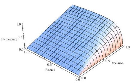
-

Рис.2 F-мера c приоритетом точности,
-

Рис.3 F-мера c приоритетом полноты,
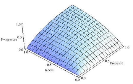
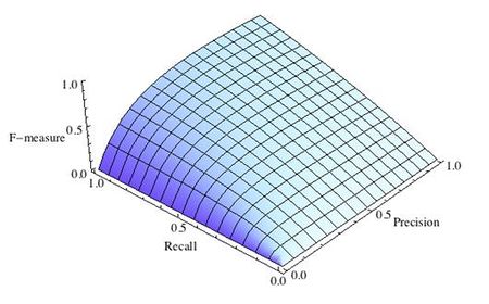
F-мера достигает максимума при максимальной полноте и точности, и близка к нулю, если один из аргументов близок к нулю.
F-мера является хорошим кандидатом на формальную метрику оценки качества классификатора. Она сводит к одному числу две других основополагающих метрики: точность и полноту. Имея «F-меру» гораздо проще ответить на вопрос: «поменялся алгоритм в лучшую сторону или нет?»
 # код для подсчета метрики F-mera:
 # Пример классификатора, способного проводить различие между всего лишь двумя
 # классами, "пятерка" и "не пятерка" из набора рукописных цифр MNIST
 import numpy as np
 from sklearn.datasets import fetch_openml
 from sklearn.model_selection import cross_val_predict
 from sklearn.linear_model import SGDClassifier
 from sklearn.metrics import f1_score
 mnist = fetch_openml('mnist_784', version=1)
 X, y = mnist["data"], mnist["target"]
 y = y.astype(np.uint8)
 X_train, X_test, y_train, y_test = X[:60000], X[60000:], y[:60000], y[60000:]
 y_train_5 = (y_train == 5) # True для всех пятерок, False для в сех остальных цифр. Задача опознать пятерки
 y_test_5 = (y_test == 5)
 sgd_clf = SGDClassifier(random_state=42) # классификатор на основе метода стохастического градиентного спуска (Stochastic Gradient Descent SGD)
 sgd_clf.fit(X_train, y_train_5) # обучаем классификатор распознавать пятерки на целом обучающем наборе
 y_train_pred = cross_val_predict(sgd_clf, X_train, y_train_5, cv=3)
 print(f1_score(y_train_5, y_train_pred))

 # 0.7325171197343846
ROC-кривая
Кривая рабочих характеристик (англ. Receiver Operating Characteristics curve).
Используется для анализа поведения классификаторов при различных пороговых значениях.
Позволяет рассмотреть все пороговые значения для данного классификатора.
Показывает долю ложно положительных примеров (англ. false positive rate, FPR) в сравнении с долей истинно положительных примеров (англ. true positive rate, TPR).
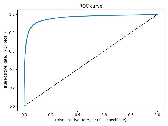
Доля FPR — это пропорция отрицательных образцов, которые были некорректно классифицированы как положительные.
- ,
где TNR — доля истинно отрицательных классификаций (англ. Тrие Negative Rate), представляющая собой пропорцию отрицательных образцов, которые были корректно классифицированы как отрицательные.
Доля TNR также называется специфичностью (англ. specificity). Следовательно, ROC-кривая изображает чувствительность (англ. seпsitivity), т.е. полноту, в сравнении с разностью 1 — specificity.
Прямая линия по диагонали представляет ROC-кривую чисто случайного классификатора. Хороший классификатор держится от указанной линии настолько далеко, насколько это
возможно (стремясь к левому верхнему углу).
Один из способов сравнения классификаторов предусматривает измерение площади под кривой (англ. Area Under the Curve — AUC). Безупречный классификатор будет иметь площадь под ROC-кривой (ROC-AUC), равную 1, тогда как чисто случайный классификатор — площадь 0.5.
 # Код отрисовки ROC-кривой
 # На примере классификатора, способного проводить различие между всего лишь двумя классами
 # "пятерка" и "не пятерка" из набора рукописных цифр MNIST
 from sklearn.metrics import roc_curve
 import matplotlib.pyplot as plt
 import numpy as np
 from sklearn.datasets import fetch_openml
 from sklearn.model_selection import cross_val_predict
 from sklearn.linear_model import SGDClassifier
 mnist = fetch_openml('mnist_784', version=1)
 X, y = mnist["data"], mnist["target"]
 y = y.astype(np.uint8)
 X_train, X_test, y_train, y_test = X[:60000], X[60000:], y[:60000], y[60000:]
 y_train_5 = (y_train == 5)  # True для всех пятерок, False для в сех остальных цифр. Задача опознать пятерки
 y_test_5 = (y_test == 5)
 sgd_clf = SGDClassifier(random_state=42) # классификатор на основе метода стохастического градиентного спуска (Stochastic Gradient Descent SGD)
 sgd_clf.fit(X_train, y_train_5) # обучаем классификатор распозновать пятерки на целом обучающем наборе
 y_train_pred = cross_val_predict(sgd_clf, X_train, y_train_5, cv=3)
 y_scores = cross_val_predict(sgd_clf, X_train, y_train_5, cv=3, method="decision_function")
 fpr, tpr, thresholds = roc_curve(y_train_5, y_scores)
 def plot_roc_curve(fpr, tpr, label=None):
     plt.plot(fpr, tpr, linewidth=2, label=label)
     plt.plot([0, 1], [0, 1], 'k--') # dashed diagonal
     plt.xlabel('False Positive Rate, FPR (1 - specificity)')
     plt.ylabel('True Positive Rate, TPR (Recall)')
     plt.title('ROC curve')
     plt.savefig("ROC.png")
 plot_roc_curve(fpr, tpr)
 plt.show()
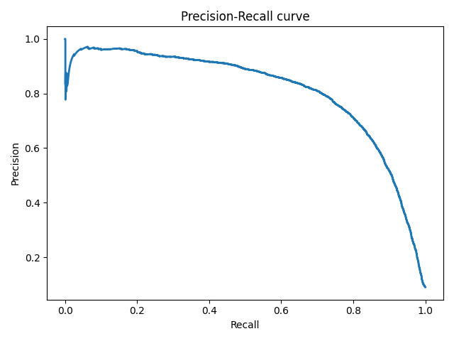
Precison-recall кривая
Чувствительность к соотношению классов.
Рассмотрим задачу выделения математических статей из множества научных статей. Допустим, что всего имеется 1.000.100 статей, из которых лишь 100 относятся к математике. Если нам удастся построить алгоритм , идеально решающий задачу, то его TPR будет равен единице, а FPR — нулю. Рассмотрим теперь плохой алгоритм, дающий положительный ответ на 95 математических и 50.000 нематематических статьях. Такой алгоритм совершенно бесполезен, но при этом имеет TPR = 0.95 и FPR = 0.05, что крайне близко к показателям идеального алгоритма.
Таким образом, если положительный класс существенно меньше по размеру, то AUC-ROC может давать неадекватную оценку качества работы алгоритма, поскольку измеряет долю неверно принятых объектов относительно общего числа отрицательных. Так, алгоритм , помещающий 100 релевантных документов на позиции с 50.001-й по 50.101-ю, будет иметь AUC-ROC 0.95.
Precison-recall (PR) кривая. Избавиться от указанной проблемы с несбалансированными классами можно, перейдя от ROC-кривой к PR-кривой. Она определяется аналогично ROC-кривой, только по осям откладываются не FPR и TPR, а полнота (по оси абсцисс) и точность (по оси ординат). Критерием качества семейства алгоритмов выступает площадь под PR-кривой (англ. Area Under the Curve — AUC-PR)
 # Код отрисовки Precison-recall кривой
 # На примере классификатора, способного проводить различие между всего лишь двумя классами
 # "пятерка" и "не пятерка" из набора рукописных цифр MNIST
 from sklearn.metrics import precision_recall_curve
 import matplotlib.pyplot as plt
 import numpy as np
 from sklearn.datasets import fetch_openml
 from sklearn.model_selection import cross_val_predict
 from sklearn.linear_model import SGDClassifier
 mnist = fetch_openml('mnist_784', version=1)
 X, y = mnist["data"], mnist["target"]
 y = y.astype(np.uint8)
 X_train, X_test, y_train, y_test = X[:60000], X[60000:], y[:60000], y[60000:]
 y_train_5 = (y_train == 5) # True для всех пятерок, False для в сех остальных цифр. Задача опознать пятерки
 y_test_5 = (y_test == 5)
 sgd_clf = SGDClassifier(random_state=42) # классификатор на основе метода стохастического градиентного спуска (Stochastic Gradient Descent SGD)
 sgd_clf.fit(X_train, y_train_5) # обучаем классификатор распозновать пятерки на целом обучающем наборе
 y_train_pred = cross_val_predict(sgd_clf, X_train, y_train_5, cv=3)
 y_scores = cross_val_predict(sgd_clf, X_train, y_train_5, cv=3, method="decision_function")
 precisions, recalls, thresholds = precision_recall_curve(y_train_5, y_scores)
 def plot_precision_recall_vs_threshold(precisions, recalls, thresholds):
     plt.plot(recalls, precisions, linewidth=2)
     plt.xlabel('Recall')
     plt.ylabel('Precision')
     plt.title('Precision-Recall curve')
     plt.savefig("Precision_Recall_curve.png")
 plot_precision_recall_vs_threshold(precisions, recalls, thresholds)
 plt.show()
Оценки качества регрессии
Наиболее типичными мерами качества в задачах регрессии являются
Средняя квадратичная ошибка (англ. Mean Squared Error, MSE)
MSE применяется в ситуациях, когда нам надо подчеркнуть большие ошибки и выбрать модель, которая дает меньше больших ошибок прогноза. Грубые ошибки становятся заметнее за счет того, что ошибку прогноза мы возводим в квадрат. И модель, которая дает нам меньшее значение среднеквадратической ошибки, можно сказать, что что у этой модели меньше грубых ошибок.
- и
Cредняя абсолютная ошибка (англ. Mean Absolute Error, MAE)
Среднеквадратичный функционал сильнее штрафует за большие отклонения по сравнению со среднеабсолютным, и поэтому более чувствителен к выбросам. При использовании любого из этих двух функционалов может быть полезно проанализировать, какие объекты вносят наибольший вклад в общую ошибку — не исключено, что на этих объектах была допущена ошибка при вычислении признаков или целевой величины.
Среднеквадратичная ошибка подходит для сравнения двух моделей или для контроля качества во время обучения, но не позволяет сделать выводов о том, на сколько хорошо данная модель решает задачу. Например, MSE = 10 является очень плохим показателем, если целевая переменная принимает значения от 0 до 1, и очень хорошим, если целевая переменная лежит в интервале (10000, 100000). В таких ситуациях вместо среднеквадратичной ошибки полезно использовать коэффициент детерминации —
Коэффициент детерминации
Коэффициент детерминации измеряет долю дисперсии, объясненную моделью, в общей дисперсии целевой переменной. Фактически, данная мера качества — это нормированная среднеквадратичная ошибка. Если она близка к единице, то модель хорошо объясняет данные, если же она близка к нулю, то прогнозы сопоставимы по качеству с константным предсказанием.
Средняя абсолютная процентная ошибка (англ. Mean Absolute Percentage Error, MAPE)
Это коэффициент, не имеющий размерности, с очень простой интерпретацией. Его можно измерять в долях или процентах. Если у вас получилось, например, что MAPE=11.4%, то это говорит о том, что ошибка составила 11,4% от фактических значений.
Основная проблема данной ошибки — нестабильность.
Корень из средней квадратичной ошибки (англ. Root Mean Squared Error, RMSE)
Примерно такая же проблема, как и в MAPE: так как каждое отклонение возводится в квадрат, любое небольшое отклонение может значительно повлиять на показатель ошибки. Стоит отметить, что существует также ошибка MSE, из которой RMSE как раз и получается путем извлечения корня.
Cимметричная MAPE (англ. Symmetric MAPE, SMAPE)
Средняя абсолютная масштабированная ошибка (англ. Mean absolute scaled error, MASE)
MASE является очень хорошим вариантом для расчета точности, так как сама ошибка не зависит от масштабов данных и является симметричной: то есть положительные и отрицательные отклонения от факта рассматриваются в равной степени.
Обратите внимание, что в MASE мы имеем дело с двумя суммами: та, что в числителе, соответствует тестовой выборке, та, что в знаменателе — обучающей. Вторая фактически представляет собой среднюю абсолютную ошибку прогноза. Она же соответствует среднему абсолютному отклонению ряда в первых разностях. Эта величина, по сути, показывает, насколько обучающая выборка предсказуема. Она может быть равна нулю только в том случае, когда все значения в обучающей выборке равны друг другу, что соответствует отсутствию каких-либо изменений в ряде данных, ситуации на практике почти невозможной. Кроме того, если ряд имеет тенденцию к росту либо снижению, его первые разности будут колебаться около некоторого фиксированного уровня. В результате этого по разным рядам с разной структурой, знаменатели будут более-менее сопоставимыми. Всё это, конечно же, является очевидными плюсами MASE, так как позволяет складывать разные значения по разным рядам и получать несмещённые оценки.
Недостаток MASE в том, что её тяжело интерпретировать. Например, MASE=1.21 ни о чём, по сути, не говорит. Это просто означает, что ошибка прогноза оказалась в 1.21 раза выше среднего абсолютного отклонения ряда в первых разностях, и ничего более.
Кросс-валидация
Хороший способ оценки модели предусматривает применение кросс-валидации (cкользящего контроля или перекрестной проверки).
В этом случае фиксируется некоторое множество разбиений исходной выборки на две подвыборки: обучающую и контрольную. Для каждого разбиения выполняется настройка алгоритма по обучающей подвыборке, затем оценивается его средняя ошибка на объектах контрольной подвыборки. Оценкой скользящего контроля называется средняя по всем разбиениям величина ошибки на контрольных подвыборках.
Примечания
- [1] Лекция «Оценивание качества» на www.coursera.org
- [2] Лекция на www.stepik.org о кросвалидации
- [3] Лекция на www.stepik.org о метриках качества, Precison и Recall
- [4] Лекция на www.stepik.org о метриках качества, F-мера
- [5] Лекция на www.stepik.org о метриках качества, примеры
См. также
- Оценка качества в задаче кластеризации
- Кросс-валидация
Источники информации
- [6] Соколов Е.А. Лекция линейная регрессия
- [7] — Дьяконов А. Функции ошибки / функционалы качества
- [8] — Оценка качества прогнозных моделей
- [9] — HeinzBr Ошибка прогнозирования: виды, формулы, примеры
- [10] — egor_labintcev Метрики в задачах машинного обучения
- [11] — grossu Методы оценки качества прогноза
- [12] — К.В.Воронцов, Классификация
- [13] — К.В.Воронцов, Скользящий контроль
What is Root Mean Square Error (RMSE)?
Root mean square error or root mean square deviation is one of the most commonly used measures for evaluating the quality of predictions. It shows how far predictions fall from measured true values using Euclidean distance.
To compute RMSE, calculate the residual (difference between prediction and truth) for each data point, compute the norm of residual for each data point, compute the mean of residuals and take the square root of that mean. RMSE is commonly used in supervised learning applications, as RMSE uses and needs true measurements at each predicted data point.
Root mean square error can be expressed as
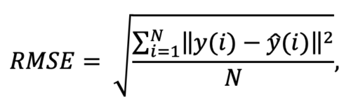
where N is the number of data points, y(i) is the i-th measurement, and y ̂(i) is its corresponding prediction.
Note: RMSE is NOT scale invariant and hence comparison of models using this measure is affected by the scale of the data. For this reason, RMSE is commonly used over standardized data.
Why is Root Mean Square Error (RMSE) Important?
In machine learning, it is extremely helpful to have a single number to judge a model’s performance, whether it be during training, cross-validation, or monitoring after deployment. Root mean square error is one of the most widely used measures for this. It is a proper scoring rule that is intuitive to understand and compatible with some of the most common statistical assumptions.
Note: By squaring errors and calculating a mean, RMSE can be heavily affected by a few predictions which are much worse than the rest. If this is undesirable, using the absolute value of residuals and/or calculating median can give a better idea of how a model performs on most predictions, without extra influence from unusually poor predictions.
How C3 AI Helps Organizations Use Root Mean Square Error (RMSE)
The C3 AI platform provides an easy way to automatically calculate RMSE and other evaluation metrics as part of a machine learning model pipeline. This extends into automated machine learning, where C3 AI® MLAutoTuner can automatically optimize hyperparameters and select model based on RMSE or other measures.

If training models is one significant aspect of machine learning, evaluating them is another. Evaluation measures how well the model fares in the presence of unseen data. It is one of the crucial metrics to determine if a model could be deemed satisfactory to proceed with.
With evaluation, we could determine if the model would build knowledge upon what it learned and apply it to data that it has never worked on before.
Take a scenario where you build an ML model using the decision tree algorithm. You procure data, initialize hyperparameters, train the model, and lastly, evaluate it. As per the evaluation results, you conclude that the decision tree algorithm isn’t as good as you assumed it to be. So you move a step ahead and apply the random forest algorithm. Result: evaluation outcome looks satisfactory.
For complex models, unlike performing evaluation once as in the previous example, evaluation might have to be done multiple times, be it with different sets of data or algorithms, to decide which model best suits your needs.
In the first part of this series, let’s understand the various regression and classification evaluation metrics that can be used to evaluate ML models.
If you want to see how these metrics can be used in action, check out our Notebook demonstrated these metrics in code form in Gradient!
Bring this project to life
Evaluation Metrics for Regression
Regression is an ML technique that outputs continuous values. For example, you may want to predict the following year’s fuel price. You build a model and train it with the fuel price dataset observed for the past few years. To evaluate your model, here are some techniques you can use:
Root Mean Squared Error
The root-mean-square deviation (RMSD) or root-mean-square error (RMSE) is used to measure the respective differences between values predicted by a model and values observed (actual values). It helps ascertain the deviation observed from actual results. Here’s how it is calculated:
[ RMSE = sqrt{sum_{i=1}^nfrac{(hat{y_i} — y_i)^2}{n}} ]
where, ( hat{y_1}, hat{y_2}, …, hat{y_n} ) are the predicted values, ( y_1, y_2, …, y_n ) are the observed values, and ( n ) is the number of predictions.
( (hat{y_i} — y_i)^2 ) is similar to the Euclidian distance formula we use to calculate the distance between two points; in our case, the predicted and observed data points.
Division by ( n ) allows us to estimate the standard deviation ( sigma ) (the deviation from the observed values) of the error for a single prediction rather than some kind of “total error” 1.
RMSE vs. MSE
- Mean squared error (MSE) is RMSE without the square root
- Since it’s squaring the prediction error, MSE is sensitive to outliers and outputs a very high value if they are present
- RMSE is preferred to MSE because MSE gives a squared error, unlike RMSE, which goes along the same units as that of the output
What’s the ideal RMSE?
First things first—the value should be small—it indicates that the model better fits the dataset. How small?
There’s no ideal value for RMSE; it depends on the range of dataset values you are working with. If the values range from 0 to 10,000, then an RMSE of say, 5.9 is said to be small and the model could be deemed satisfactory, whereas, if the range is from 0 to 10, an RMSE of 5.9 is said to be poor, and the model may need to be tweaked.
Mean Absolute Error
The mean absolute error (MAE) is the mean of the absolute values of prediction errors. We use absolute because without doing so the negative and positive errors would cancel out; we instead use MAE to find the overall magnitude of the error. The prediction error is the difference between observed and predicted values.
[ MAE = frac{1}{n} sum_{i=1}^{n} |hat{y_i} — y_i| ]
where ( hat{y_i} ) is the prediction value, and ( y_i ) is the observed value.
RMSE vs. MAE
- MAE is a linear score where all the prediction errors are weighted equally, unlike RMSE, which squares the prediction errors and applies a square root to the average
- In general, RMSE score will always be higher than or equal to MAE
- If outliers are not meant to be penalized heavily, MAE is a good choice
- If large errors are undesirable, RMSE is useful because it gives a relatively high weight to large errors
Root Mean Squared Log Error
When the square root is applied to the mean of the squared logarithmic differences between predicted and observed values, we get root mean squared log error (RMSLE).
[ RMSLE = sqrt{frac{1}{n} sum_{i=1}^{n} (log(hat{y_i} + 1) — log(y_i + 1))^2} ]
where ( hat{y_i} ) is the prediction value, and ( y_i ) is the observed value.
Choosing RMSLE vs. RMSE
- If outliers are not to be penalized, RMSLE is a good choice because RMSE can explode the outlier to a high value
- RMSLE computes relative error where the scale of the error is not important
- RMLSE incurs a hefty penalty for the underestimation of the actual value2
R Squared
R-squared (also called the coefficient of determination) represents the goodness-of-fit measure for regression models. It gives the proportion of variance in the target variable (dependent variable) that the independent variables explain collectively.
R-squared evaluates the scatter of data points around the best fit line. It can be formulated as:
[ R^2 = frac{var(mean) — var(line)}{var(mean)} ]
where ( var(mean) ) is the variance with respect to mean, and var(line) is the variance concerning the best fit line. The ( R^2 ) value can help relate ( var(mean) ) against the ( var(line) ). If ( R^2 ) is, say, 0.83, it means that there is 83% less variation around the line than the mean, i.e., the relationship between independent variables and the target variable accounts for 83% of the variation3.
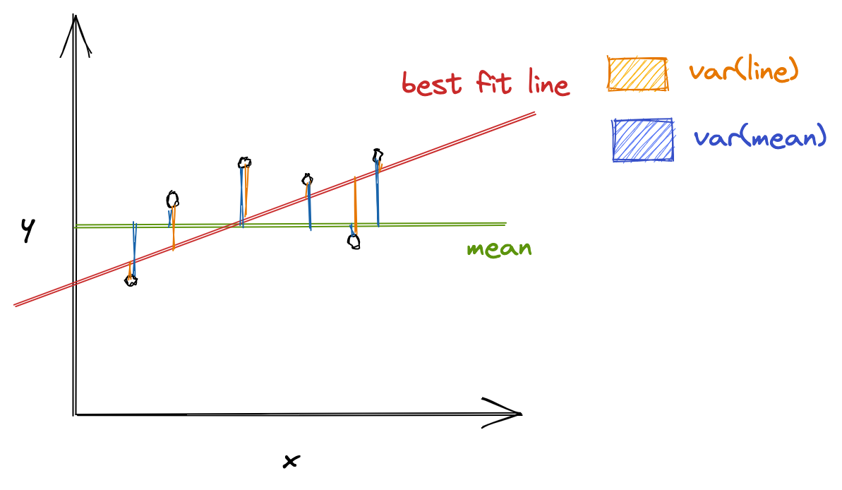
The higher the R-squared value, the better the model. 0% means that the model does not explain any variance of the target variable around its mean, whereas 100% means that the model explains all variations in the target variable around its mean.
RMSE vs. R Squared
It’s better to compute both the metrics because RMSE calculates the distance between predicted and observed values, whereas, R-squared tells how well the predictor variables (the data attributes) can explain the variation in the target variable.
Limitations
R-squared doesn’t always present an accurate value to conclude if the model is good. For example, if the model is biased, R-squared can be pretty high, which isn’t reflective of the biased data. Hence, it is always advisable to use R-squared with other stats and residual plots for context4.
Evaluation Metrics for Classification
Classification is a technique to identify class labels for a given dataset. Consider a scenario where you want to classify an automobile as excellent/good/bad. You then could train a model on a dataset containing information about both the automobile of interest and other classes of vehicle, and verify the model is effective using classification metrics to evaluate the model’s performance. To analyze the credibility of your classification model on test/validation datasets, techniques that you can use are as follows:
Accuracy
Accuracy is the percentage of correct predictions for the test data. It is computed as follows:
[ accuracy = frac{correct, predictions}{all, predictions} ]
In classification, the meta metrics we usually use to compute our metrics are:
- True Positives (TP): Prediction belongs to a class, and observed belongs to a class as well
- True Negatives (TN): Prediction doesn’t belong to a class and observation doesn’t belong to that class
- False Positives (FP): Prediction belongs to a class, but observation doesn’t belong to that class
- False Negatives (FN): Prediction doesn’t belong to a class, but observation belongs to a class
All meta metrics can be arranged in a matrix as follows:
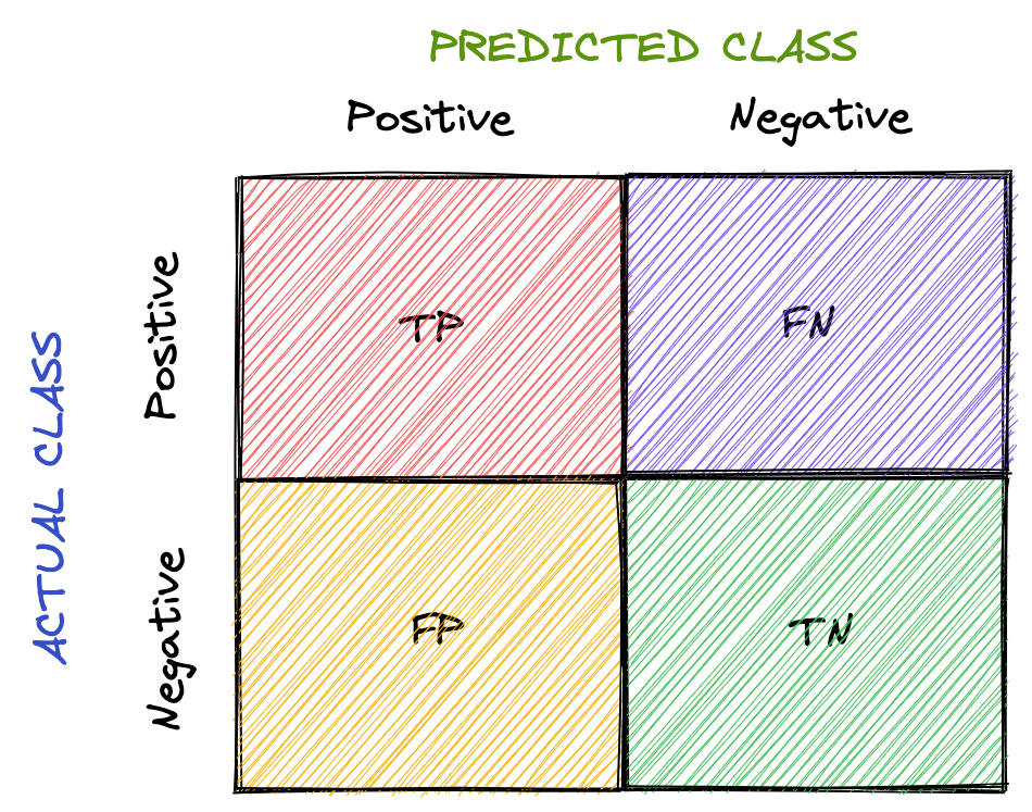
This is called the confusion matrix. It gives a visual representation of the algorithm’s performance.
For multiclass classification, we would have more rows and columns, denoting the dataset’s classes.
Now let’s rework our accuracy formula using the meta metrics.
[ accuracy = frac{TP + TN}{TP + TN + FP + FN} ]
( TP + TN ) is used because ( TP + TN ) together denote the correct predictions.
Limitations
Accuracy might not always be a good performance indicator. For example, in the case of cancer detection, the cost of failing to diagnose cancer is much higher than the cost of diagnosing cancer in a person who doesn’t have cancer. If the accuracy here is said to be 90%, we are missing out on the other 10% who might have cancer.
Overall, accuracy depends on the problem in consideration. Along with accuracy, you might want to think about other classification metrics to evaluate your model.
Precision
Precision is defined as the fraction of correctly classified samples among all data points that are predicted to belong to a certain class. In general, it translates to “how many of our predictions to belong to a certain class are correct”.
[ precision = frac{TP}{TP + FP} ]
To understand precision, let’s consider the cancer detection problem again. If “having cancer” is a positive class, meta metrics are as follows:
( TP ) = prediction: having cancer, actual (observed): having cancer
( FP ) = prediction: having cancer, actual: not having cancer
Thus, ( frac{TP}{TP + FP} ) gives the measure of how well our prediction fares, i.e., it measures how many people diagnosed with cancer have cancer and helps ensure we don’t misclassify people not having cancer as having cancer.
Recall
Recall (also called sensitivity) is defined as the fraction of samples predicted to belong to a class among all data points that actually belong to a class. In general, it translates to “how many data points that belong to a class are correctly classified”.
[ recall = frac{TP}{TP + FN} ]
Considering the cancer detection problem, if “having cancer” is a positive class, meta metrics are as follows:
( TP ): prediction: having cancer, actual (observed): having cancer
( FN ): prediction: not having cancer, actual: having cancer
Thus, ( frac{TP}{TP + FN} ) measures how well classification has been done with respect to a class, i.e., it measures how many people with cancer are diagnosed with cancer, and helps ensure that cancer doesn’t go undetected.
F-Measure
Since precision and recall capture different properties of the model, it’s sometimes beneficial to compute both metrics together. In situations where both metrics bear consideration, how about we have precision and recall in a single metric?
F-Measure (also called F1-Measure) comes to the rescue. It is the harmonic mean of precision and recall.
[ F-Measure = frac{2}{frac{1}{recall} + frac{1}{precision}} = 2 * frac{precision * recall}{precision + recall} ]
A generalized F-measure is ( F_beta ), which is given as:
[ F_beta = (1 + beta ^2) * frac{precision * recall}{(beta^2 * precision) + recall} ]
where ( beta ) is chosen such that recall is considered ( beta ) times as important as precision5.
Specificity
Specificity is defined as the fraction of samples predicted to not belong to a class among all data points that actually do not belong to a class. In general, it translates to “how many data points that do not belong to a class are correctly classified”.
[ specificity = frac{TN}{TN + FP} ]
Considering the cancer detection problem, if “having cancer” is a positive class, meta metrics are as follows:
( TN ): prediction: not having cancer, actual (observed): not having cancer
( FP ): prediction: having cancer, actual: not having cancer
Thus, ( frac{TN}{TN + FP} ) measures how well classification has been done with respect to a class, i.e., it measures how many people not having cancer are predicted as not having cancer.
ROC
The receiver operating characteristic (ROC) curve plots recall (true positive rate) and false-positive rate.
[ TPR = frac{TP}{TP + FN} ]
[ FPR = frac{FP}{FP + TN} ]
The area under ROC (AUC) measures the entire area under the curve. The higher the AUC, the better the classification model.

For example, if the AUC is 0.8, it means there is an 80% chance that the model will be able to distinguish between positive and negative classes.
PR
The precision-recall (PR) curve plots precision and recall. When it comes to imbalanced classification, the PR curve could be helpful. The resulting curve could belong to any of the following tiers:
- High precision and recall: A higher area under the PR curve indicates high precision and recall, which means that the model is performing well by generating accurate predictions (precision: model detects cancer; indeed, has cancer) and correctly classifying samples belonging to a certain class (recall: has cancer, accurately diagnoses cancer).
- High precision and low recall: The model detects cancer, and the person indeed has cancer; however, it misses a lot of actual «has cancer» samples.
- Low precision and high recall: The model gives a lot of «has cancer» and «not having cancer» predictions. It thinks a lot of «has cancer» class samples as «not having cancer»; however, it also misclassifies many «has cancer» when «not having cancer» is the suitable class.
- Low precision and low recall: Neither the classification is done right, nor the samples belonging to a specific class are predicted correctly.
ROC vs. PR
- ROC curve can be used when the dataset is not imbalanced because despite the dataset being imbalanced, ROC presents an overly optimistic picture of the model’s performance
- PR curve should be used when the dataset is imbalanced
In this article, you got to know several evaluation metrics that can evaluate regression and classification models.
The caveat here could be that not every evaluation metric can be independently relied on; to conclude if a model is performing well, we may consider a group of metrics.
Besides evaluation metrics, the other measures that one could focus on to check if an ML model is acceptable include:
- Compare your model’s score with other similar models and verify if your model’s performance is on par with them
- Keep an eye out for Bias and variance to verify if a model generalizes well
- Cross-validation
In the next part, let’s dig into the evaluation metrics for clustering and ranking models.
Notebooks detailing the material covered above can be found on Github here.
In the previous post, we saw the various metrics which are used to assess a machine learning model’s performance. Among those, the confusion matrix is used to evaluate a classification problem’s accuracy. On the other hand, mean squared error (MSE), and mean absolute error (MAE) are used to evaluate the regression problem’s accuracy.
F1 score is useful when the size of the positive class is relatively small.
ROC Area Under Curve is useful when we are not concerned about whether the small dataset/class of dataset is positive or not, in contrast to F1 score where the class being positive is important.

In today’s post, we will understand what MAE is and explore more about what it means to vary these metrics. In addition to this, we will discuss a few more metrics that will help us decide if the machine learning model would be useful in real-life scenarios or not.
1. Mean Absolute Error or MAE
We know that an error basically is the absolute difference between the actual or true values and the values that are predicted. Absolute difference means that if the result has a negative sign, it is ignored.
Hence, MAE = True values – Predicted values
MAE takes the average of this error from every sample in a dataset and gives the output.
This can be implemented using sklearn’s mean_absolute_error method:
from sklearn.metrics import mean_absolute_error

# predicting home prices in some area
predicted_home_prices = mycity_model.predict(X)
mean_absolute_error(y, predicted_home_prices)
But this value might not be the relevant aspect that can be considered while dealing with a real-life situation because the data we use to build the model as well as evaluate it is the same, which means the model has no exposure to real, never-seen-before data. So, it may perform extremely well on seen data but might fail miserably when it encounters real, unseen data.
The concepts of underfitting and overfitting can be pondered over, from here:
Underfitting: The scenario when a machine learning model almost exactly matches the training data but performs very poorly when it encounters new data or validation set.
Overfitting: The scenario when a machine learning model is unable to capture the important patterns and insights from the data, which results in the model performing poorly on training data itself.
P.S. In the upcoming posts, we will understand how to fit the model in the right way using many methods like feature normalization, feature generation and much more.
2. Mean Squared Error or MSE
MSE is calculated by taking the average of the square of the difference between the original and predicted values of the data.
Hence, MSE = 
Here N is the total number of observations/rows in the dataset. The sigma symbol denotes that the difference between actual and predicted values taken on every i value ranging from 1 to n.
This can be implemented using sklearn‘s mean_squared_error method:
from sklearn.metrics import mean_squared_error

actual_values = [3, -0.5, 2, 7]
predicted_values = [2.5, 0.0, 2, 8]

mean_squared_error(actual_values, predicted_values)
In most of the regression problems, mean squared error is used to determine the model’s performance.
3. Root Mean Squared Error or RMSE
RMSE is the standard deviation of the errors which occur when a prediction is made on a dataset. This is the same as MSE (Mean Squared Error) but the root of the value is considered while determining the accuracy of the model.
from sklearn.metrics import mean_squared_error
from math import sqrt

actual_values = [3, -0.5, 2, 7]
predicted_values = [2.5, 0.0, 2, 8]

mean_squared_error(actual_values, predicted_values)
# taking root of mean squared error
root_mean_squared_error = sqrt(mean_squared_error)
4. R Squared
It is also known as the coefficient of determination. This metric gives an indication of how good a model fits a given dataset. It indicates how close the regression line (i.e the predicted values plotted) is to the actual data values. The R squared value lies between 0 and 1 where 0 indicates that this model doesn’t fit the given data and 1 indicates that the model fits perfectly to the dataset provided.
import numpy as np

X = np.random.randn(100)
y = np.random.randn(60) # y has nothing to do with X whatsoever

from sklearn.linear_model import LinearRegression
from sklearn.cross_validation import cross_val_score

scores = cross_val_score(LinearRegression(), X, y,scoring='r2')
Where to use which Metric to determine the Performance of a Machine Learning Model?
MAE: It is not very sensitive to outliers in comparison to MSE since it doesn’t punish huge errors. It is usually used when the performance is measured on continuous variable data. It gives a linear value, which averages the weighted individual differences equally. The lower the value, better is the model’s performance.
MSE: It is one of the most commonly used metrics, but least useful when a single bad prediction would ruin the entire model’s predicting abilities, i.e when the dataset contains a lot of noise. It is most useful when the dataset contains outliers, or unexpected values (too high or too low values).
RMSE: In RMSE, the errors are squared before they are averaged. This basically implies that RMSE assigns a higher weight to larger errors. This indicates that RMSE is much more useful when large errors are present and they drastically affect the model’s performance. It avoids taking the absolute value of the error and this trait is useful in many mathematical calculations. In this metric also, the lower the value, better is the performance of the model.
You may also like:
- How Good is my Machine Learning Model? How do I improve its Performance?
- Machine Learning — How to deal with missing data using Python?
- Machine Learning and Data Visualization using Orange
- Designing a Learning System | The first step to Machine Learning
- Главная
- Вопросы и ответы
Среднеквадратичная ошибка (RMSE)
Краткая объяснение что такое RMSE применительно к данным ДЗЗ
Обсудить в форуме Комментариев — 1
Среднеквадратичная ошибка (Root Mean Square Error, RMS Error, RMSE) — расстояние между двумя точками.
В случае если речь идет о привязке данных, в качестве точек между которыми измеряется расстояние могут выступать:
- Исходная точка и конечная точки (например результат трансформации), в этом случае RMSE будет показателем насколько исходная точка близка к конечной — текущая ошибка.
- Желаемое положение выходной точки (точка поставленная пользователем) и результатом ее трансформации (точка поставленная моделью). Трансформация — то или иное математическое преобразование исходных координат в конечные, примером такого преобразования может быть аффинная или полиномиальная трансформация. В данном случае RMSE показывает насколько используемая трансформация позволяет точно приблизить исходную точку к конечной, т.е. RMSE в этом случае — ошибка трансформации.
Как видно на иллюстрации ниже, выходные точки 1, 2, 3 поставленные оператором (синие) совпадают с трансформированными (расчетными) значениями (зеленые) и не видны из-за точного совпадения, а вот точка 4 поставлена не там, куда бы она попала используя ту же трансформацию, это дает возможность вычислить для нее RMSE, для точек 1, 2, 3 RMSE = 0.
Привязываемое изображение слева, изображение используемое в качестве источника координат (привязанное) справа.
Примечание: здесь и далее в статье, как и в ERDAS IMAGINE Field Guide, RMS определяется как расстояние (длина гипотенузы), что не совсем соответствует определению Root Mean Squared, так как отсутствует компонент усреднения, классический RMS должен вычисляться делением выражения под корнем на N измерений, в этом случае на 2. В данном случае удобнее называть RMS — расстоянием.
Ошибка RMS рассчитывается по следующей формуле, представляющей из себя формулу вычисления расстояния:
где xi, yi — исходные координаты, xr, yr — конечные координаты
RMSE выражается как расстояние в единицах исходной системы координат, то есть, если вы привязываете только что отсканированную карту, то RMSE будет выражаться в пикселях (или долях пикселя), если вы производите дополнительную привязку снимка, то RMSE будет показывать значения в метрах. Значение RMSE равное 2 для определенной точки будет означать, что ее исходная координата удалена на 2 пикселя или метра от конечной (расчетной) точки.
Чтобы лучше понять когда и как можно получить RMSE при привязке можно использовать следующий алгоритм, иллюстрирующую процесс привязки с помощью аффинного преобразования:
- Получение изображения, например сканированием, изображение получает пиксельную систему координат X,Y (колонка, ряд).
- Расстановка трех точек с начальными и конечными координатами. Эти координаты указывают:
- Начальные координаты — положение точки на непривязанном материале (координаты конкретного пиксела по системе ряд/колонка);
- Конечные координаты — положение точки на привязанном материале, любом источнике координат, географических или спроектированных.
- Три точки — минимальное количество, необходимое для того, чтобы решить систему уравнений аффинного преобразования:
x0 = a+ b*x + c*y
y0 = d + e*x + f*yРешение уравнения заключается в нахождении всех шести коэффициентов, например решением системы уравнений:
x1′ = a + b*x1 + c*y1
y1′ = d + e*x1 + f*y1
x2′ = a + b*x2 + c*y2
y2′ = d + e*x2 + f*y2
x3′ = a + b*x3 + c*y3
y3′ = d + e*x3 + f*y3Если точек меньше чем минимально необходимо — решить систему невозможно, нельзя найти коэффициенты трансформации и соответственно невозможно произвести пересчет координат. RMSE для точек также вычислить невозможно.
- Расстановка минимально необходимого количества точек для данного преобразования (трех) приводит к тому, что RMSE для каждой точки становится равна 0. Можно производить трансформацию. Однако в таком случае мы не можем сделать выводов о качестве точек, ведь для этого надо рассчитать RMSE, а значит….
- Ставим дополнительные точки. Появление новых данных как правило приводит к тому, что то положение, куда мы ставим конечную точку в процессе привязки и ее расчетное положение не совпадают. Это делает возможным расчет RMS ошибки.
С примером и математикой расчета полиномиального преобразования 2-ой степени можно прочитать в статье «Полиномиальные преобразования — вычисления и практика».
Помимо RMSE часто также можно увидеть также значения ошибки по одной из осей X или Y. Эти значения являются остатками (residuals) и могут быть рассчитаны для каждой точки. Изучение значений этих ошибок может помочь понять, почему привязанный материал смещен по одной из осей. Это проблема часто возникает при привязке данных полученных при съемке под углом (не в надир).
Уравнение вычисления RMS для каждой точки можно переписать как:
![]()
где XR и YR — остаточные ошибки по X и Y соответственно.
Графически ошибки по X и Y, а также RMSE соотносятся следующим образом:
Вычислив RMSE для каждой точки, можно также определить общую ошибку по X (Rx), Y (Ry) и общую RMSE (T) используя следующие формулы:
где n — число контрольных точек, i — порядковый номер контрольной точки, d — расстояние между парой точек.
Связь со средним расстоянием
Другим, достаточно объективным, способом оценить точность привязки является среднее расстояние, которое очень похоже по формуле на RMSE, но является менее консервативным показателем, так как расстояния не возводятся в квадрат как в RMSE. Выразив расстояние через d, приведем для сравнения формулы вычисления общей RMSE (T) и среднего расстояния (MD):
RMSE является более общеупотребимым в литературе.
Другим распространенным способом описания точности набора измерений являются квантили дробные стандартному отклонению (сигма).
Вклад точки в общую RMSE
Для того, чтобы вычислить вклад точки в общую ошибку (Ei), необходимо разделить RMSE этой точки (Ri) на общую RMSE.

Допуск RMSE
В большинстве случаев, вместо того, чтобы усложнять тип трансформации (например переходить к более высоким порядкам полиномиальных преобразований) имеет смысл допустить некоторую ошибку. Величину допустимой RMSE можно представить как окно, окружающее точку с желаемыми координатами, положением расчетной точки внутри которого считается корректным. Например, если допуск RMSE равен 2, то расчетный пиксел может находится в двух пикселях от указанного оператором и являться допустимым. Величина допустимой ошибки зависит от типа и точности данных, задачи и точности контрольных точек.
Важно помнить, что RMSE указывается в пикселях, поэтому, если привязываются данные Landsat имеющие разрешение 30 метров и задача осуществить привязку с точностью не меньше тех же 30 метров, то RMSE не должна превышать 1.00 (пикселя).
Оценка RMSE
Если RMSE расчитана и найдена слишком высокой, есть 4 варианта решения проблемы:
- Найти и удалить контрольные точки с большой RMSE, подразумевая, что это наименее точные точки. Это чревато еще возникновением еще больших ошибок, если отбраковываемая точка — единственная на большой участок изображения.
- Увеличить допуск RMSE.
- Увеличить сложность функции трансформации, которая более точно будет соответствовать введенным точкам. RMSE точек при этом уменьшится, однако использование сложных криволинейных функций может привести к нежелательным сильным искажениям растра.
- Оставить только точки в которых Вы уверены, что они правильны.
В статье использованы материалы ERDAS IMAGINE Field Guide
Обсудить в форуме Комментариев — 1
Последнее обновление: September 09 2021
Дата создания: 27.07.2007
Автор(ы): Максим Дубинин