Obviously it is of great importance to understand and utilize the metrics properly also in machine learning. Deriving insights without making clear sense of metrics is like choosing between 1 litre of milk and 0.6 galon of milk. If we dont know well the metrics litre and galon we can’t make an healty decision.
In this notebook we talk about the regression model metrics:
- Mean Squared Error ($MSE$)
- R-Squared ($R^2$)
- Root Mean Squared Logarithmic Error ($RMSLE$)
We will later add new metrics to this notebook by time.

R-Squared ( $R^2$) and Mean Squared Error ($MSE$)
-
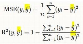
$MSE$ measures how far the data are from the model’s predicted values
-
$R^2$ measures how far the data are from the model’s predicted values compare to how far the data are from the mean
-
The difference between how far the data are from the model’s predicted values and how far the data are from the mean is the improvement in prediction from the regression model.
$MSE$
- Sensitive to outliers
- Has the same units as the response variable.
- Lower values of $MSE$ indicate better fit.
- Actually, it’s hard to realize if our model is good or not by looking at the absolute values of $MSE$ or $MSE$.
- We would probably want to measure how much our model is better than the constant baseline.
Disadvantage of MSE:
- If we make a single very bad prediction, taking the square will make the error even worse and
- it may skew the metric towards overestimating the model’s badness.
- That is a particularly problematic behaviour if we have noisy data (data that for whatever reason is not entirely reliable)
- On the other hand, if all the errors are smaller than 1, than it affects in the opposite direction: we may underestimate the model’s badness.
$R^2$
-
proportional improvement in prediction of the regression model, compared to the mean model (model predicting all given samples as mean value).
-
interpreted as the proportion of total variance that is explained by the model.
-
relative measure of fit whereas $MSE$ is an absolute measure of fit
- often easier to interpret since it doesn’t depend on the scale of the data.
- It doesn’t matter if the output values are very large or very small,
-
always has values between
-∞and1. -
There are situations in which a high $R^2$ is not necessary or relevant.
- When the interest is in the relationship between variables, not in prediction, the $R^2$ is less important.
Root Mean Squared Logaritmic Error (RMSLE)
Mechanism:
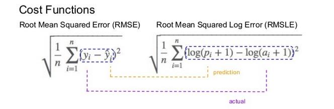
- It is the Root Mean Squared Error of the log-transformed predicted and log-transformed actual values.
-
RMSLEadds1to both actual and predicted values before taking the natural logarithm to avoid taking the natural log of possible0 (zero)values. -
As a result, the function can be used if actual or predicted have zero-valued elements. But this function is not appropriate if either is negative valued
Functionality:
-
The expression $$ log(p_i +1) − log(a_i+1)$$ can be written as $$ log((p_i+1) / (a_i+1)) $$
-
RMSLE measures the ratio of predicted and actual.
RMSLE is preferable when
- targets having exponential growth, such as population counts, average sales of a commodity over a span of years etc
- we care about percentage errors rather than the absolute value of errors.
- there is a wide range in the target variables and
- we don’t want to penalize big differences when both the predicted and the actual are big numbers.
- we want to penalize under estimates more than over estimates.
Let’s imagine two cases of predictions,
- Case-1: our model makes a prediction of
30when the actual number is40 -
Case-2: our model makes a prediction of
300when the actual number is400- With RMSE the second result is scored as
10 timesmore than the first result - Conversely, with RMSLogE two results are scored the same.
- RMSLogE takes into account just the ratio of change
- With RMSE the second result is scored as
Lets have a look at the below example
-
Case-3 :
-
Prediction = $600$, Actual = $1000$ (the absolute difference is $400$)
-
RMSE = $400$,
- RMSLogE = $0.5108$
-
-
Case-4 :
-
Prediction = $1400$, Actual = $1000$ (the absolute difference is $400$)
-
RMSE = $400$,
- RMSLogE = $0.3365$
-
- When the differences are the same between actual and predicted in both cases.
- RMSE treated them equally, however
- RMSLogE penalized the under estimate more than over estimate (under estimated prediction score is higher than over estimated prediction score)
- Often, penalizing the under estimate more than over estimate is important for prediction of sales and inventory demands.
- To some extent having extra inventory or supply might be more preferable to not being able to providing product as much as the demand.
Для того чтобы модель линейной регрессии можно было применять на практике необходимо сначала оценить её качество. Для этих целей предложен ряд показателей, каждый из которых предназначен для использования в различных ситуациях и имеет свои особенности применения (линейные и нелинейные, устойчивые к аномалиям, абсолютные и относительные, и т.д.). Корректный выбор меры для оценки качества модели является одним из важных факторов успеха в решении задач анализа данных.
- Среднеквадратичная ошибка (Mean Squared Error)
- Корень из среднеквадратичной ошибки (Root Mean Squared Error)
- Среднеквадратичная ошибка в процентах (Mean Squared Percentage Error)
- Cредняя абсолютная ошибка (Mean Absolute Error)
- Средняя абсолютная процентная ошибка (Mean Absolute Percentage Error)
- Cимметричная средняя абсолютная процентная ошибка (Symmetric Mean Absolute Percentage Error)
- Средняя абсолютная масштабированная ошибка (Mean absolute scaled error)
- Средняя относительная ошибка (Mean Relative Error)
- Среднеквадратичная логарифмическая ошибка (Root Mean Squared Logarithmic Error
- R-квадрат
- Скорректированный R-квадрат
- Сравнение метрик
«Хорошая» аналитическая модель должна удовлетворять двум, зачастую противоречивым, требованиям — как можно лучше соответствовать данным и при этом быть удобной для интерпретации пользователем. Действительно, повышение соответствия модели данным как правило связано с её усложнением (в случае регрессии — увеличением числа входных переменных модели). А чем сложнее модель, тем ниже её интерпретируемость.
Поэтому при выборе между простой и сложной моделью последняя должна значимо увеличивать соответствие модели данным чтобы оправдать рост сложности и соответствующее снижение интерпретируемости. Если это условие не выполняется, то следует выбрать более простую модель.
Таким образом, чтобы оценить, насколько повышение сложности модели значимо увеличивает её точность, необходимо использовать аппарат оценки качества регрессионных моделей. Он включает в себя следующие меры:
- Среднеквадратичная ошибка (MSE).
- Корень из среднеквадратичной ошибки (RMSE).
- Среднеквадратичная ошибка в процентах (MSPE).
- Средняя абсолютная ошибка (MAE).
- Средняя абсолютная ошибка в процентах (MAPE).
- Cимметричная средняя абсолютная процентная ошибка (SMAPE).
- Средняя абсолютная масштабированная ошибка (MASE)
- Средняя относительная ошибка (MRE).
- Среднеквадратичная логарифмическая ошибка (RMSLE).
- Коэффициент детерминации R-квадрат.
- Скорректированный коэффициент детеминации.
Прежде чем перейти к изучению метрик качества, введём некоторые базовые понятия, которые нам в этом помогут. Для этого рассмотрим рисунок.
Рисунок 1. Линейная регрессия
Наклонная прямая представляет собой линию регрессии с переменной, на которой расположены точки, соответствующие предсказанным значениям выходной переменной widehat{y} (кружки синего цвета). Оранжевые кружки представляют фактические (наблюдаемые) значения y . Расстояния между ними и линией регрессии — это ошибка предсказания модели y-widehat{y} (невязка, остатки). Именно с её использованием вычисляются все приведённые в статье меры качества.
Горизонтальная линия представляет собой модель простого среднего, где коэффициент при независимой переменной x равен нулю, и остаётся только свободный член b, который становится равным среднему арифметическому фактических значений выходной переменной, т.е. b=overline{y}. Очевидно, что такая модель для любого значения входной переменной будет выдавать одно и то же значение выходной — overline{y}.
В линейной регрессии такая модель рассматривается как «бесполезная», хуже которой работает только «случайный угадыватель». Однако, она используется для оценки, насколько дисперсия фактических значений y относительно линии среднего, больше, чем относительно линии регрессии с переменной, т.е. насколько модель с переменной лучше «бесполезной».
MSE
Среднеквадратичная ошибка (Mean Squared Error) применяется в случаях, когда требуется подчеркнуть большие ошибки и выбрать модель, которая дает меньше именно больших ошибок. Большие значения ошибок становятся заметнее за счет квадратичной зависимости.
Действительно, допустим модель допустила на двух примерах ошибки 5 и 10. В абсолютном выражении они отличаются в два раза, но если их возвести в квадрат, получив 25 и 100 соответственно, то отличие будет уже в четыре раза. Таким образом модель, которая обеспечивает меньшее значение MSE допускает меньше именно больших ошибок.
MSE рассчитывается по формуле:
MSE=frac{1}{n}sumlimits_{i=1}^{n}(y_{i}-widehat{y}_{i})^{2},
где n — количество наблюдений по которым строится модель и количество прогнозов, y_{i} — фактические значение зависимой переменной для i-го наблюдения, widehat{y}_{i} — значение зависимой переменной, предсказанное моделью.
Таким образом, можно сделать вывод, что MSE настроена на отражение влияния именно больших ошибок на качество модели.
Недостатком использования MSE является то, что если на одном или нескольких неудачных примерах, возможно, содержащих аномальные значения будет допущена значительная ошибка, то возведение в квадрат приведёт к ложному выводу, что вся модель работает плохо. С другой стороны, если модель даст небольшие ошибки на большом числе примеров, то может возникнуть обратный эффект — недооценка слабости модели.
RMSE
Корень из среднеквадратичной ошибки (Root Mean Squared Error) вычисляется просто как квадратный корень из MSE:
RMSE=sqrt{frac{1}{n}sumlimits_{i=1}^{n}(y_{i}-widehat{y_{i}})^{2}}
MSE и RMSE могут минимизироваться с помощью одного и того же функционала, поскольку квадратный корень является неубывающей функцией. Например, если у нас есть два набора результатов работы модели, A и B, и MSE для A больше, чем MSE для B, то мы можем быть уверены, что RMSE для A больше RMSE для B. Справедливо и обратное: если MSE(A)<MSE(B), то и RMSE(A)<RMSE(B).
Следовательно, сравнение моделей с помощью RMSE даст такой же результат, что и для MSE. Однако с MSE работать несколько проще, поэтому она более популярна у аналитиков. Кроме этого, имеется небольшая разница между этими двумя ошибками при оптимизации с использованием градиента:
frac{partial RMSE}{partial widehat{y}_{i}}=frac{1}{2sqrt{MSE}}frac{partial MSE}{partial widehat{y}_{i}}
Это означает, что перемещение по градиенту MSE эквивалентно перемещению по градиенту RMSE, но с другой скоростью, и скорость зависит от самой оценки MSE. Таким образом, хотя RMSE и MSE близки с точки зрения оценки моделей, они не являются взаимозаменяемыми при использовании градиента для оптимизации.
Влияние каждой ошибки на RMSE пропорционально величине квадрата ошибки. Поэтому большие ошибки оказывают непропорционально большое влияние на RMSE. Следовательно, RMSE можно считать чувствительной к аномальным значениям.
MSPE
Среднеквадратичная ошибка в процентах (Mean Squared Percentage Error) представляет собой относительную ошибку, где разность между наблюдаемым и фактическим значениями делится на наблюдаемое значение и выражается в процентах:
MSPE=frac{100}{n}sumlimits_{i=1}^{n}left ( frac{y_{i}-widehat{y}_{i}}{y_{i}} right )^{2}
Проблемой при использовании MSPE является то, что, если наблюдаемое значение выходной переменной равно 0, значение ошибки становится неопределённым.
MSPE можно рассматривать как взвешенную версию MSE, где вес обратно пропорционален квадрату наблюдаемого значения. Таким образом, при возрастании наблюдаемых значений ошибка имеет тенденцию уменьшаться.
MAE
Cредняя абсолютная ошибка (Mean Absolute Error) вычисляется следующим образом:
MAE=frac{1}{n}sumlimits_{i=1}^{n}left | y_{i}-widehat{y}_{i} right |
Т.е. MAE рассчитывается как среднее абсолютных разностей между наблюдаемым и предсказанным значениями. В отличие от MSE и RMSE она является линейной оценкой, а это значит, что все ошибки в среднем взвешены одинаково. Например, разница между 0 и 10 будет вдвое больше разницы между 0 и 5. Для MSE и RMSE, как отмечено выше, это не так.
Поэтому MAE широко используется, например, в финансовой сфере, где ошибка в 10 долларов должна интерпретироваться как в два раза худшая, чем ошибка в 5 долларов.
MAPE
Средняя абсолютная процентная ошибка (Mean Absolute Percentage Error) вычисляется следующим образом:
MAPE=frac{100}{n}sumlimits_{i=1}^{n}frac{left | y_{i}-widehat{y_{i}} right |}{left | y_{i} right |}
Эта ошибка не имеет размерности и очень проста в интерпретации. Её можно выражать как в долях, так и в процентах. Если получилось, например, что MAPE=11.4, то это говорит о том, что ошибка составила 11.4% от фактического значения.
SMAPE
Cимметричная средняя абсолютная процентная ошибка (Symmetric Mean Absolute Percentage Error) — это мера точности, основанная на процентных (или относительных) ошибках. Обычно определяется следующим образом:
SMAPE=frac{100}{n}sumlimits_{i=1}^{n}frac{left | y_{i}-widehat{y_{i}} right |}{(left | y_{i} right |+left | widehat{y}_{i} right |)/2}
Т.е. абсолютная разность между наблюдаемым и предсказанным значениями делится на полусумму их модулей. В отличие от обычной MAPE, симметричная имеет ограничение на диапазон значений. В приведённой формуле он составляет от 0 до 200%. Однако, поскольку диапазон от 0 до 100% гораздо удобнее интерпретировать, часто используют формулу, где отсутствует деление знаменателя на 2.
Одной из возможных проблем SMAPE является неполная симметрия, поскольку в разных диапазонах ошибка вычисляется неодинаково. Это иллюстрируется следующим примером: если y_{i}=100 и widehat{y}_{i}=110, то SMAPE=4.76, а если y_{i}=100 и widehat{y}_{i}=90, то SMAPE=5.26.
Ограничение SMAPE заключается в том, что, если наблюдаемое или предсказанное значение равно 0, ошибка резко возрастет до верхнего предела (200% или 100%).
MASE
Средняя абсолютная масштабированная ошибка (Mean absolute scaled error) — это показатель, который позволяет сравнивать две модели. Если поместить MAE для новой модели в числитель, а MAE для исходной модели в знаменатель, то полученное отношение и будет равно MASE. Если значение MASE меньше 1, то новая модель работает лучше, если MASE равно 1, то модели работают одинаково, а если значение MASE больше 1, то исходная модель работает лучше, чем новая модель. Формула для расчета MASE имеет вид:
MASE=frac{MAE_{i}}{MAE_{j}}
MASE симметрична и устойчива к выбросам.
MRE
Средняя относительная ошибка (Mean Relative Error) вычисляется по формуле:
MRE=frac{1}{n}sumlimits_{i=1}^{n}frac{left | y_{i}-widehat{y}_{i}right |}{left | y_{i} right |}
Несложно увидеть, что данная мера показывает величину абсолютной ошибки относительно фактического значения выходной переменной (поэтому иногда эту ошибку называют также средней относительной абсолютной ошибкой, MRAE). Действительно, если значение абсолютной ошибки, скажем, равно 10, то сложно сказать много это или мало. Например, относительно значения выходной переменной, равного 20, это составляет 50%, что достаточно много. Однако относительно значения выходной переменной, равного 100, это будет уже 10%, что является вполне нормальным результатом.
Очевидно, что при вычислении MRE нельзя применять наблюдения, в которых y_{i}=0.
Таким образом, MRE позволяет более адекватно оценить величину ошибки, чем абсолютные ошибки. Кроме этого она является безразмерной величиной, что упрощает интерпретацию.
RMSLE
Среднеквадратичная логарифмическая ошибка (Root Mean Squared Logarithmic Error) представляет собой RMSE, вычисленную в логарифмическом масштабе:
RMSLE=sqrt{frac{1}{n}sumlimits_{i=1}^{n}(log(widehat{y}_{i}+1)-log{(y_{i}+1}))^{2}}
Константы, равные 1, добавляемые в скобках, необходимы чтобы не допустить обращения в 0 выражения под логарифмом, поскольку логарифм нуля не существует.
Известно, что логарифмирование приводит к сжатию исходного диапазона изменения значений переменной. Поэтому применение RMSLE целесообразно, если предсказанное и фактическое значения выходной переменной различаются на порядок и больше.
R-квадрат
Перечисленные выше ошибки не так просто интерпретировать. Действительно, просто зная значение средней абсолютной ошибки, скажем, равное 10, мы сразу не можем сказать хорошая это ошибка или плохая, и что нужно сделать чтобы улучшить модель.
В этой связи представляет интерес использование для оценки качества регрессионной модели не значения ошибок, а величину показывающую, насколько данная модель работает лучше, чем модель, в которой присутствует только константа, а входные переменные отсутствуют или коэффициенты регрессии при них равны нулю.
Именно такой мерой и является коэффициент детерминации (Coefficient of determination), который показывает долю дисперсии зависимой переменной, объяснённой с помощью регрессионной модели. Наиболее общей формулой для вычисления коэффициента детерминации является следующая:
R^{2}=1-frac{sumlimits_{i=1}^{n}(widehat{y}_{i}-y_{i})^{2}}{sumlimits_{i=1}^{n}({overline{y}}_{i}-y_{i})^{2}}
Практически, в числителе данного выражения стоит среднеквадратическая ошибка оцениваемой модели, а в знаменателе — модели, в которой присутствует только константа.
Главным преимуществом коэффициента детерминации перед мерами, основанными на ошибках, является его инвариантность к масштабу данных. Кроме того, он всегда изменяется в диапазоне от −∞ до 1. При этом значения близкие к 1 указывают на высокую степень соответствия модели данным. Очевидно, что это имеет место, когда отношение в формуле стремится к 0, т.е. ошибка модели с переменными намного меньше ошибки модели с константой. R^{2}=0 показывает, что между независимой и зависимой переменными модели имеет место функциональная зависимость.
Когда значение коэффициента близко к 0 (т.е. ошибка модели с переменными примерно равна ошибке модели только с константой), это указывает на низкое соответствие модели данным, когда модель с переменными работает не лучше модели с константой.
Кроме этого, бывают ситуации, когда коэффициент R^{2} принимает отрицательные значения (обычно небольшие). Это произойдёт, если ошибка модели среднего становится меньше ошибки модели с переменной. В этом случае оказывается, что добавление в модель с константой некоторой переменной только ухудшает её (т.е. регрессионная модель с переменной работает хуже, чем предсказание с помощью простой средней).
На практике используют следующую шкалу оценок. Модель, для которой R^{2}>0.5, является удовлетворительной. Если R^{2}>0.8, то модель рассматривается как очень хорошая. Значения, меньшие 0.5 говорят о том, что модель плохая.
Скорректированный R-квадрат
Основной проблемой при использовании коэффициента детерминации является то, что он увеличивается (или, по крайней мере, не уменьшается) при добавлении в модель новых переменных, даже если эти переменные никак не связаны с зависимой переменной.
В связи с этим возникают две проблемы. Первая заключается в том, что не все переменные, добавляемые в модель, могут значимо увеличивать её точность, но при этом всегда увеличивают её сложность. Вторая проблема — с помощью коэффициента детерминации нельзя сравнивать модели с разным числом переменных. Чтобы преодолеть эти проблемы используют альтернативные показатели, одним из которых является скорректированный коэффициент детерминации (Adjasted coefficient of determinftion).
Скорректированный коэффициент детерминации даёт возможность сравнивать модели с разным числом переменных так, чтобы их число не влияло на статистику R^{2}, и накладывает штраф за дополнительно включённые в модель переменные. Вычисляется по формуле:
R_{adj}^{2}=1-frac{sumlimits_{i=1}^{n}(widehat{y}_{i}-y_{i})^{2}/(n-k)}{sumlimits_{i=1}^{n}({overline{y}}_{i}-y_{i})^{2}/(n-1)}
где n — число наблюдений, на основе которых строится модель, k — количество переменных в модели.
Скорректированный коэффициент детерминации всегда меньше единицы, но теоретически может принимать значения и меньше нуля только при очень малом значении обычного коэффициента детерминации и большом количестве переменных модели.
Сравнение метрик
Резюмируем преимущества и недостатки каждой приведённой метрики в следующей таблице:
| Мера | Сильные стороны | Слабые стороны |
|---|---|---|
| MSE | Позволяет подчеркнуть большие отклонения, простота вычисления. | Имеет тенденцию занижать качество модели, чувствительна к выбросам. Сложность интерпретации из-за квадратичной зависимости. |
| RMSE | Простота интерпретации, поскольку измеряется в тех же единицах, что и целевая переменная. | Имеет тенденцию занижать качество модели, чувствительна к выбросам. |
| MSPE | Нечувствительна к выбросам. Хорошо интерпретируема, поскольку имеет линейный характер. | Поскольку вклад всех ошибок отдельных наблюдений взвешивается одинаково, не позволяет подчёркивать большие и малые ошибки. |
| MAPE | Является безразмерной величиной, поэтому её интерпретация не зависит от предметной области. | Нельзя использовать для наблюдений, в которых значения выходной переменной равны нулю. |
| SMAPE | Позволяет корректно работать с предсказанными значениями независимо от того больше они фактического, или меньше. | Приближение к нулю фактического или предсказанного значения приводит к резкому росту ошибки, поскольку в знаменателе присутствует как фактическое, так и предсказанное значения. |
| MASE | Не зависит от масштаба данных, является симметричной: положительные и отрицательные отклонения от фактического значения учитываются одинаково. Устойчива к выбросам. Позволяет сравнивать модели. | Сложность интерпретации. |
| MRE | Позволяет оценить величину ошибки относительно значения целевой переменной. | Неприменима для наблюдений с нулевым значением выходной переменной. |
| RMSLE | Логарифмирование позволяет сделать величину ошибки более устойчивой, когда разность между фактическим и предсказанным значениями различается на порядок и выше | Может быть затруднена интерпретация из-за нелинейности. |
| R-квадрат | Универсальность, простота интерпретации. | Возрастает даже при включении в модель бесполезных переменных. Плохо работает когда входные переменные зависимы. |
| R-квадрат скорр. | Корректно отражает вклад каждой переменной в модель. | Плохо работает, когда входные переменные зависимы. |
В данной статье рассмотрены наиболее популярные меры качества регрессионных моделей, которые часто используются в различных аналитических приложениях. Эти меры имеют свои особенности применения, знание которых позволит обоснованно выбирать и корректно применять их на практике.
Однако в литературе можно встретить и другие меры качества моделей регрессии, которые предлагаются различными авторами для решения конкретных задач анализа данных.
Другие материалы по теме:
Отбор переменных в моделях линейной регрессии
Репрезентативность выборочных данных
Логистическая регрессия и ROC-анализ — математический аппарат
If training models is one significant aspect of machine learning, evaluating them is another. Evaluation measures how well the model fares in the presence of unseen data. It is one of the crucial metrics to determine if a model could be deemed satisfactory to proceed with.
With evaluation, we could determine if the model would build knowledge upon what it learned and apply it to data that it has never worked on before.
Take a scenario where you build an ML model using the decision tree algorithm. You procure data, initialize hyperparameters, train the model, and lastly, evaluate it. As per the evaluation results, you conclude that the decision tree algorithm isn’t as good as you assumed it to be. So you move a step ahead and apply the random forest algorithm. Result: evaluation outcome looks satisfactory.
For complex models, unlike performing evaluation once as in the previous example, evaluation might have to be done multiple times, be it with different sets of data or algorithms, to decide which model best suits your needs.
In the first part of this series, let’s understand the various regression and classification evaluation metrics that can be used to evaluate ML models.
If you want to see how these metrics can be used in action, check out our Notebook demonstrated these metrics in code form in Gradient!
Bring this project to life
Evaluation Metrics for Regression
Regression is an ML technique that outputs continuous values. For example, you may want to predict the following year’s fuel price. You build a model and train it with the fuel price dataset observed for the past few years. To evaluate your model, here are some techniques you can use:
Root Mean Squared Error
The root-mean-square deviation (RMSD) or root-mean-square error (RMSE) is used to measure the respective differences between values predicted by a model and values observed (actual values). It helps ascertain the deviation observed from actual results. Here’s how it is calculated:
[ RMSE = sqrt{sum_{i=1}^nfrac{(hat{y_i} — y_i)^2}{n}} ]
where, ( hat{y_1}, hat{y_2}, …, hat{y_n} ) are the predicted values, ( y_1, y_2, …, y_n ) are the observed values, and ( n ) is the number of predictions.
( (hat{y_i} — y_i)^2 ) is similar to the Euclidian distance formula we use to calculate the distance between two points; in our case, the predicted and observed data points.
Division by ( n ) allows us to estimate the standard deviation ( sigma ) (the deviation from the observed values) of the error for a single prediction rather than some kind of “total error” 1.
RMSE vs. MSE
- Mean squared error (MSE) is RMSE without the square root
- Since it’s squaring the prediction error, MSE is sensitive to outliers and outputs a very high value if they are present
- RMSE is preferred to MSE because MSE gives a squared error, unlike RMSE, which goes along the same units as that of the output
What’s the ideal RMSE?
First things first—the value should be small—it indicates that the model better fits the dataset. How small?
There’s no ideal value for RMSE; it depends on the range of dataset values you are working with. If the values range from 0 to 10,000, then an RMSE of say, 5.9 is said to be small and the model could be deemed satisfactory, whereas, if the range is from 0 to 10, an RMSE of 5.9 is said to be poor, and the model may need to be tweaked.
Mean Absolute Error
The mean absolute error (MAE) is the mean of the absolute values of prediction errors. We use absolute because without doing so the negative and positive errors would cancel out; we instead use MAE to find the overall magnitude of the error. The prediction error is the difference between observed and predicted values.
[ MAE = frac{1}{n} sum_{i=1}^{n} |hat{y_i} — y_i| ]
where ( hat{y_i} ) is the prediction value, and ( y_i ) is the observed value.
RMSE vs. MAE
- MAE is a linear score where all the prediction errors are weighted equally, unlike RMSE, which squares the prediction errors and applies a square root to the average
- In general, RMSE score will always be higher than or equal to MAE
- If outliers are not meant to be penalized heavily, MAE is a good choice
- If large errors are undesirable, RMSE is useful because it gives a relatively high weight to large errors
Root Mean Squared Log Error
When the square root is applied to the mean of the squared logarithmic differences between predicted and observed values, we get root mean squared log error (RMSLE).
[ RMSLE = sqrt{frac{1}{n} sum_{i=1}^{n} (log(hat{y_i} + 1) — log(y_i + 1))^2} ]
where ( hat{y_i} ) is the prediction value, and ( y_i ) is the observed value.
Choosing RMSLE vs. RMSE
- If outliers are not to be penalized, RMSLE is a good choice because RMSE can explode the outlier to a high value
- RMSLE computes relative error where the scale of the error is not important
- RMLSE incurs a hefty penalty for the underestimation of the actual value2
R Squared
R-squared (also called the coefficient of determination) represents the goodness-of-fit measure for regression models. It gives the proportion of variance in the target variable (dependent variable) that the independent variables explain collectively.
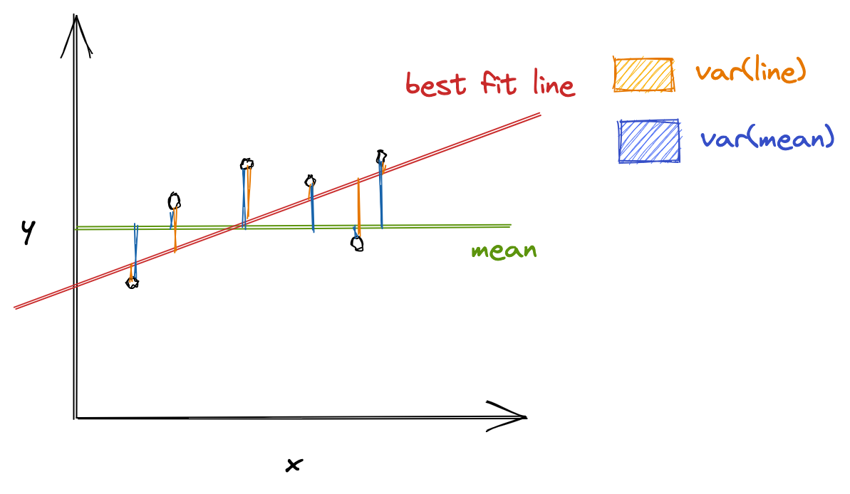
R-squared evaluates the scatter of data points around the best fit line. It can be formulated as:
[ R^2 = frac{var(mean) — var(line)}{var(mean)} ]
where ( var(mean) ) is the variance with respect to mean, and var(line) is the variance concerning the best fit line. The ( R^2 ) value can help relate ( var(mean) ) against the ( var(line) ). If ( R^2 ) is, say, 0.83, it means that there is 83% less variation around the line than the mean, i.e., the relationship between independent variables and the target variable accounts for 83% of the variation3.
The higher the R-squared value, the better the model. 0% means that the model does not explain any variance of the target variable around its mean, whereas 100% means that the model explains all variations in the target variable around its mean.
RMSE vs. R Squared
It’s better to compute both the metrics because RMSE calculates the distance between predicted and observed values, whereas, R-squared tells how well the predictor variables (the data attributes) can explain the variation in the target variable.
Limitations
R-squared doesn’t always present an accurate value to conclude if the model is good. For example, if the model is biased, R-squared can be pretty high, which isn’t reflective of the biased data. Hence, it is always advisable to use R-squared with other stats and residual plots for context4.
Evaluation Metrics for Classification
Classification is a technique to identify class labels for a given dataset. Consider a scenario where you want to classify an automobile as excellent/good/bad. You then could train a model on a dataset containing information about both the automobile of interest and other classes of vehicle, and verify the model is effective using classification metrics to evaluate the model’s performance. To analyze the credibility of your classification model on test/validation datasets, techniques that you can use are as follows:
Accuracy
Accuracy is the percentage of correct predictions for the test data. It is computed as follows:
[ accuracy = frac{correct, predictions}{all, predictions} ]
In classification, the meta metrics we usually use to compute our metrics are:
- True Positives (TP): Prediction belongs to a class, and observed belongs to a class as well
- True Negatives (TN): Prediction doesn’t belong to a class and observation doesn’t belong to that class
- False Positives (FP): Prediction belongs to a class, but observation doesn’t belong to that class
- False Negatives (FN): Prediction doesn’t belong to a class, but observation belongs to a class
All meta metrics can be arranged in a matrix as follows:
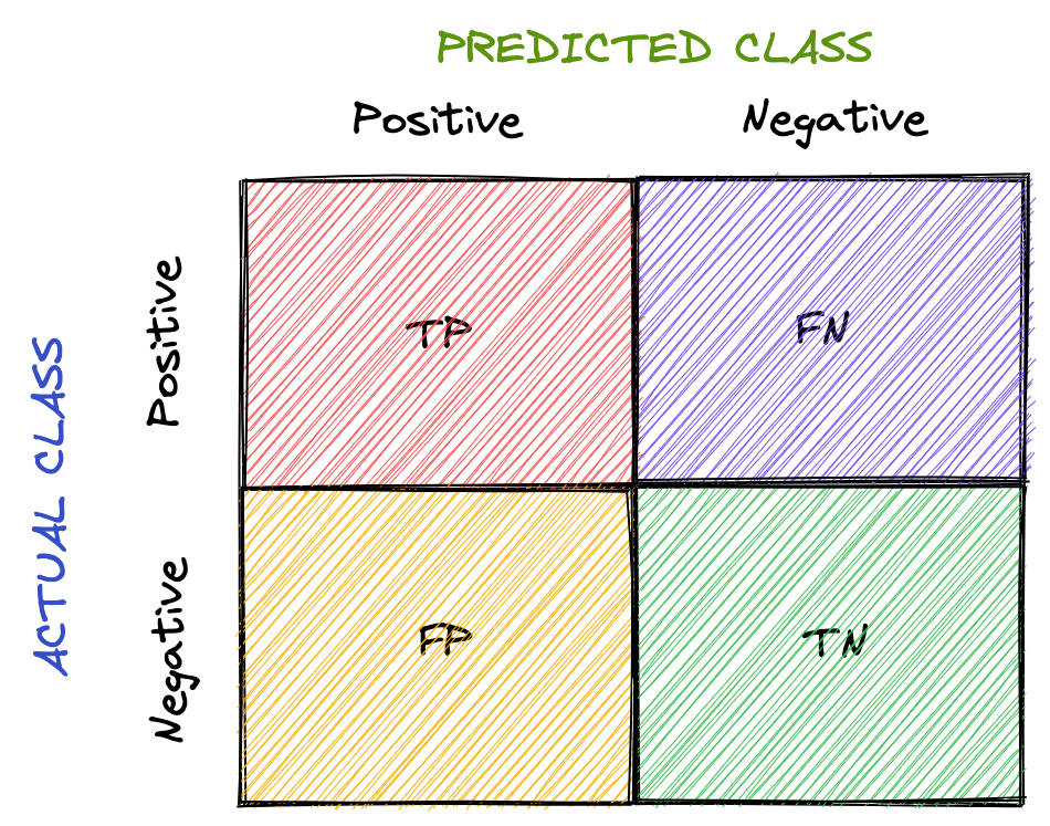
This is called the confusion matrix. It gives a visual representation of the algorithm’s performance.
For multiclass classification, we would have more rows and columns, denoting the dataset’s classes.
Now let’s rework our accuracy formula using the meta metrics.
[ accuracy = frac{TP + TN}{TP + TN + FP + FN} ]
( TP + TN ) is used because ( TP + TN ) together denote the correct predictions.
Limitations
Accuracy might not always be a good performance indicator. For example, in the case of cancer detection, the cost of failing to diagnose cancer is much higher than the cost of diagnosing cancer in a person who doesn’t have cancer. If the accuracy here is said to be 90%, we are missing out on the other 10% who might have cancer.
Overall, accuracy depends on the problem in consideration. Along with accuracy, you might want to think about other classification metrics to evaluate your model.
Precision
Precision is defined as the fraction of correctly classified samples among all data points that are predicted to belong to a certain class. In general, it translates to “how many of our predictions to belong to a certain class are correct”.
[ precision = frac{TP}{TP + FP} ]
To understand precision, let’s consider the cancer detection problem again. If “having cancer” is a positive class, meta metrics are as follows:
( TP ) = prediction: having cancer, actual (observed): having cancer
( FP ) = prediction: having cancer, actual: not having cancer
Thus, ( frac{TP}{TP + FP} ) gives the measure of how well our prediction fares, i.e., it measures how many people diagnosed with cancer have cancer and helps ensure we don’t misclassify people not having cancer as having cancer.
Recall
Recall (also called sensitivity) is defined as the fraction of samples predicted to belong to a class among all data points that actually belong to a class. In general, it translates to “how many data points that belong to a class are correctly classified”.
[ recall = frac{TP}{TP + FN} ]
Considering the cancer detection problem, if “having cancer” is a positive class, meta metrics are as follows:
( TP ): prediction: having cancer, actual (observed): having cancer
( FN ): prediction: not having cancer, actual: having cancer
Thus, ( frac{TP}{TP + FN} ) measures how well classification has been done with respect to a class, i.e., it measures how many people with cancer are diagnosed with cancer, and helps ensure that cancer doesn’t go undetected.
F-Measure
Since precision and recall capture different properties of the model, it’s sometimes beneficial to compute both metrics together. In situations where both metrics bear consideration, how about we have precision and recall in a single metric?
F-Measure (also called F1-Measure) comes to the rescue. It is the harmonic mean of precision and recall.
[ F-Measure = frac{2}{frac{1}{recall} + frac{1}{precision}} = 2 * frac{precision * recall}{precision + recall} ]
A generalized F-measure is ( F_beta ), which is given as:
[ F_beta = (1 + beta ^2) * frac{precision * recall}{(beta^2 * precision) + recall} ]
where ( beta ) is chosen such that recall is considered ( beta ) times as important as precision5.
Specificity
Specificity is defined as the fraction of samples predicted to not belong to a class among all data points that actually do not belong to a class. In general, it translates to “how many data points that do not belong to a class are correctly classified”.
[ specificity = frac{TN}{TN + FP} ]
Considering the cancer detection problem, if “having cancer” is a positive class, meta metrics are as follows:
( TN ): prediction: not having cancer, actual (observed): not having cancer
( FP ): prediction: having cancer, actual: not having cancer
Thus, ( frac{TN}{TN + FP} ) measures how well classification has been done with respect to a class, i.e., it measures how many people not having cancer are predicted as not having cancer.
ROC
The receiver operating characteristic (ROC) curve plots recall (true positive rate) and false-positive rate.
[ TPR = frac{TP}{TP + FN} ]
[ FPR = frac{FP}{FP + TN} ]
The area under ROC (AUC) measures the entire area under the curve. The higher the AUC, the better the classification model.

For example, if the AUC is 0.8, it means there is an 80% chance that the model will be able to distinguish between positive and negative classes.
PR
The precision-recall (PR) curve plots precision and recall. When it comes to imbalanced classification, the PR curve could be helpful. The resulting curve could belong to any of the following tiers:
- High precision and recall: A higher area under the PR curve indicates high precision and recall, which means that the model is performing well by generating accurate predictions (precision: model detects cancer; indeed, has cancer) and correctly classifying samples belonging to a certain class (recall: has cancer, accurately diagnoses cancer).
- High precision and low recall: The model detects cancer, and the person indeed has cancer; however, it misses a lot of actual «has cancer» samples.
- Low precision and high recall: The model gives a lot of «has cancer» and «not having cancer» predictions. It thinks a lot of «has cancer» class samples as «not having cancer»; however, it also misclassifies many «has cancer» when «not having cancer» is the suitable class.
- Low precision and low recall: Neither the classification is done right, nor the samples belonging to a specific class are predicted correctly.
ROC vs. PR
- ROC curve can be used when the dataset is not imbalanced because despite the dataset being imbalanced, ROC presents an overly optimistic picture of the model’s performance
- PR curve should be used when the dataset is imbalanced
In this article, you got to know several evaluation metrics that can evaluate regression and classification models.
The caveat here could be that not every evaluation metric can be independently relied on; to conclude if a model is performing well, we may consider a group of metrics.
Besides evaluation metrics, the other measures that one could focus on to check if an ML model is acceptable include:
- Compare your model’s score with other similar models and verify if your model’s performance is on par with them
- Keep an eye out for Bias and variance to verify if a model generalizes well
- Cross-validation
In the next part, let’s dig into the evaluation metrics for clustering and ranking models.
Notebooks detailing the material covered above can be found on Github here.
![]()
![]()
Machine learning & Data Science course
Explore machine learning, data science, business analysis & product management mini courses. Click on the link below
![]()
![]()
If you are working on a regression-based machine learning model like linear regression, one of the most important tasks is to select an appropriate evaluation metric.
In fact, if you are working on a machine learning projects in general or preparing to become a data scientist, it’s kind of must for you to know the top evaluation metrics.
These are also called loss functions.
There are two kinds of machine learning problems – classification and regression.
And these have different kind of loss functions.
In this post, I am going to talk about regression’s loss functions.
Since every project or data set is different, we must select appropriate evaluation metrics. Usually, more than 1 metrics is required to evaluate a machine learning model.
Instead of including all the loss functions or evaluation metrics for regression machine learning models, I will try to focus on top loss functions.
Download android app for better experience.
Evaluation Metrics or Loss functions for Regression
Before we start with loss functions, you need to understand what we are trying to do here. In a typical regression-based machine learning model, our model will produce continuous values (predicted value).
Our primary objective is to keep these predicted values closer to actual values.
Predicted values are denoted by y hat ().
Actual values are denoted by y.
Error = y — y hat
")
So, whenever we are talking about error in this post, we are talking about this error. And yes, ideal condition (hypothetical one) is that this error (difference) is 0, which means our model can predict all values correctly (which is not going to happen).
Let’s start with mean absolute error.
Mean absolute error (MAE)
In simple terms, mean absolute error is the sum of absolute/positive errors of all values. So, if there are 5 values in our data set, we find out the difference between the actual value and predicted values for all 5 values and take their positive value. So even if the difference between actual and predicted value is negative, we take positive value for calculation.
So we take the positive value of all errors, add them and find out their mean.
Mean absolute error illustration;
|
Actual Value (y) |
Predicted Value (y hat) |
Error (difference) |
Absolute Error |
|
|
100 |
130 |
-30 |
30 |
|
|
150 |
170 |
-20 |
20 |
|
|
200 |
220 |
-20 |
20 |
|
|
250 |
260 |
-10 |
10 |
|
|
300 |
325 |
-25 |
25 |
|
|
21 |
Mean |
|||
|
Note— You take the absolute value of error which is the positive value, therefore -30 becomes 30 |
||||
MAE is the sum of absolute differences between actual and predicted values. It doesn’t consider the direction, that is, positive or negative.
When we consider directions also, that is called Mean Bias Error (MBE), which is a sum of errors(difference).
Formula for mean absolute Error or MAE is represented by;
")
Mean Square Error (MSE)
Mean square error is always positive and a value closer to 0 or a lower value is better. Let’s see how this this is calculated;
")
Let’s use the last illustration to understand it better.
|
Actual Value (y) |
Predicted Value (y hat) |
Error (difference) |
Squared Error |
|
|---|---|---|---|---|
|
100 |
130 |
-30 |
900 |
|
|
150 |
170 |
-20 |
400 |
|
|
200 |
220 |
-20 |
400 |
|
|
250 |
260 |
-10 |
100 |
|
|
300 |
325 |
-25 |
625 |
|
|
485 |
Mean |
So if we were to run a model with different parameters/independent variables, model with lower MSE will be deemed better.
We will look at its comparison with other loss functions in a while in this post. First quickly cover RMSE.
Root mean square error (RMSE)
Square root of MSE yields root mean square error (RMSE). So it’s formula is quite similar to what you have seen with mean square error, it’s just that we need to add a square root sign to it;
")
It is the standard deviation of error (residual error).
it indicates the spread of the residual errors. It is always positive, and a lower value indicates better performance. Ideal value would be 0 but it is never achieved.
|
Actual Value (y) |
Predicted Value (y hat) |
Error (difference) |
Squared Error |
|
|
100 |
130 |
-30 |
900 |
|
|
150 |
170 |
-20 |
400 |
|
|
200 |
220 |
-20 |
400 |
|
|
250 |
260 |
-10 |
100 |
|
|
300 |
325 |
-25 |
625 |
|
|
485 |
Mean |
|||
|
22.02271555 |
Square root of mean |
Effect of each error on RMSE is directly proportional to the squared error therefore, RMSE is sensitive to outliers and can exaggerate results if there are outliers in the data set.
Before moving to their comparison, I just want to mention one more evaluation metric and that is Root mean squared log error (RMSLE)
Root mean squared log error (RMSLE)
Root mean squared log error is basically RMSE but calculated at logarithmic scale. So, if you understand the above mentioned 3 evaluation metrics, you won’t have any problem understanding RMSLE or most other evaluation metric or loss functions used in regression-based machine learning model.
While calculating RMSLE, 1 is added as constant to actual and predicted values because they can be 0 and log of 0 is undefined. Overall formula remains same. Standard denotation for RMSLE is;

In this illustration, I have used log for calculation;
|
Actual Value (y) |
Predicted Value (y hat) |
Actual + 1 |
Predicted + 1 |
log (Actual) |
Log (Predicted) |
Error (difference) |
Squared Error |
|
|
100 |
130 |
101 |
131 |
2.004321374 |
2.117271296 |
-0.112949922 |
0.012757685 |
|
|
150 |
170 |
151 |
171 |
2.178976947 |
2.23299611 |
-0.054019163 |
0.00291807 |
|
|
200 |
220 |
201 |
221 |
2.303196057 |
2.344392274 |
-0.041196216 |
0.001697128 |
|
|
250 |
260 |
251 |
261 |
2.399673721 |
2.416640507 |
-0.016966786 |
0.000287872 |
|
|
300 |
325 |
301 |
326 |
2.478566496 |
2.5132176 |
-0.034651104 |
0.001200699 |
|
|
0.003772291 |
Mean |
|||||||
|
0.061418977 |
Squre root of mean |
Let’s look their difference now.
MAE vs MSE vs RMSE Vs RMSLE
In terms of comparison, primary differences are between MAE & MSE because they both are calculated in different ways. RMSE & RMSLE are extension of MSE therefore they share lots of properties with MSE.
|
Mean absolute Error (MAE) |
Mean square Error (MSE) |
Root mean square error (RMSE) |
Root mean square log Error (RMSLE) |
|
It doesn’t account for the direction of the value. Even if value is negative, positive value is used for calculation. |
It does account for positive or negative value. |
It does account for positive or negative value. |
It does account for positive or negative value. |
|
RMSE & MSE share many properties with MSE because RMSE is simply the square root of MSE. |
RMSE & MSE share many properties with MSE because it is simply the square root of MSE. |
||
|
MAE is less biased for higher values. It may not adequately reflect the performance when dealing with large error values. |
MSE is highly biased for higher values. |
RMSE is better in terms of reflecting performance when dealing with large error values. |
|
|
RMSE is more useful when lower residual values are preferred. |
|||
|
MAE is less than RMSE as the sample size goes up. |
RMSE tends to be higher than MAE as the sample size goes up. |
||
|
MAE doesn’t necessarily penalize large errors. |
MSE penalize large errors. |
RMSE penalize large errors. |
RMSLE doesn’t penalize large errors. It is usually used when you don’t want to influence the results if there are large errors. RMSLE penalize lower errors. |
|
MAE is more useful when the overall impact is proportionate to the actual increase in error. For example- if error values go up to 6 from 3, actual impact on the result is twice. It is more common in financial industry where a loss of 6 would be twice of 3. |
RMSE is more useful when the overall impact is disproportionate to the actual increase in error. For example- if error values go up to 6 from 3, actual impact on the result is more than twice. This could be common in clinical trials, as error goes up, overall impact goes up disproportionately. |
||
|
When actual and predicted values are low, RMSE & RMSLE are usually same. |
When actual and predicted values are low, RMSE & RMSLE are usually same. |
||
|
When either of actual or predicted values are high, RMSE > RMSLE. |
When either of actual or predicted values are high, RMSE > RMSLE. |
MAE vs MSE vs RMSE Vs RMSLE Conclusion
I have mentioned only important differences. If there is no valid point for one, I haven’t included in the above table and that’s why we have empty cells in the table.
Few important points to remember when using loss functions for your regression;
- Never compare apple with oranges, that is, never compare different metrics with each other. For example- don’t compare values of MSE with MAE or others. They would be different.
- Try to use more than 1 loss function.
- Always calculate evaluation metrics (loss functions) for both testing and training data set.
- Compare evaluation metrics between test and training data set. There shouldn’t be a huge difference between them. If there is, there is a problem with your model. For example- if you are using RMSE, calculate RMSE for testing and training data set. There should be huge difference between these values for this data set.
- If you have outlier in the data and you want to ignore them, MAE is a better option but if you want to account for them in your loss function, go for MSE/RMSE.
Questions or feedback? Please leave your comments.
While crafting machine learning model there is always need to asses its performance. When trying multiple models or hyper parameter tuning it is useful to compare different approaches and choose the best one. The sklearn.metrics provides plethora of metrics for suitable for distinct purposes.
In this series of posts I will discuss four groups of common machine learning tasks each requires specific metrics:
- Regression — predict value of one or more variables that are continuous, e.g. predict stock price of given asset or predict temperature for next day.
- Binary classification — assign sample to one of two classes — example: classify image as one containing «cat» or «dog»
- Multiple class classification — assign sample to one of many classes example: classify new article to category «sport», «politics», «economy», «pop-culture»,…
- Other
The Kaggle competitions give insight into approach taken by Kaggle team to select best evaluation metrics for given task. There use to be Kaggle wiki under containing short definitions of metrics used in Kaggle competitions but it is not available anymore. In this post we will look closer at the first group and explain few model evaluation metrics used in regression problems. Here metrics that are discussed in this post.
- Absolute Error — AE
- Mean Absolute Error — MAE
- Weighted Mean Absolute Error — WMAE
- Pearson Correlation Coefficient
- Spearman’s Rank Correlation
- Root Mean Squared Error — RMSE
- Root Mean Squared Logarithmic Error — RMSLE
- Mean Columnwise Root Mean Squared Error — MCRMSE
- References
Absolute Error — AE
The sum of the absolute value of each individual error.
$$
mathrm{AE} = sum_{i=1}^n | y_i — hat{y}_i |
$$
Where:
(mathrm{AE} = |e_i| = |y_i-hat{y_i}|),
(n) — number test of samples,
(y_i) — actual variable value,
(hat{y}_i) — predicted variable value.
MAE can cause notable difference between public and private leaderboard calculations. One drawback of the Absolute Error metrics is that direct comparison of the metrics for model used to predict variables on different scales is not possible. E.g. when using model to financial predictions of S&P 500 index and using the same model to predict value of Microsoft stock price we cannot compare their performance using this metrics since units and ranges are different. The S&P 500 is expressed in points and stock price of asset is expressed in dollars. In this situation one can use (percentage error) to get evaluation metrics in common scale.
Exemplary competition using Mean Absolute Error for model evaluation:
- Forecast Eurovision Voting — This competition requires contestants to forecast the voting for this year’s Eurovision Song Contest in Norway on May 25th, 27th and 29th.
Mean Absolute Error — MAE
Mean of the absolute value of each individual error.
The mean absolute error (MAE) is a quantity used to measure how close forecasts or predictions are to the eventual outcomes. The mean absolute error is given by formula:
$$
mathrm{MAE} = frac{1}{n}sum_{i=1}^n left| y_i — hat{y_i}right| =frac{1}{n}sum_{i=1}^n left| e_i right|.
$$
Where:
(n) — number test of samples,
(y_i) — actual variable value,
(hat{y}_i) — predicted variable value.
see also paper: Advantages of the mean absolute error (MAE) over the root mean square error (RMSE) in assessing average model performance
Five exemplary competitions using Mean Absolute Error for model evaluation:
-
LANL Earthquake Prediction — Can you predict upcoming laboratory earthquakes?
-
PUBG Finish Placement Prediction — Can you predict the battle royale finish of PUBG Players?
-
Allstate Claims Severity — How severe is an insurance claim?
-
Loan Default Prediction — Imperial College London — Constructing an optimal portfolio of loans.
-
Finding Elo — Predict a chess player’s FIDE Elo rating from one game.
Weighted Mean Absolute Error — WMAE
Weighted average of absolute errors.
WMAE can be used as evaluation tool for better assessing the model performance with respect to the goals of the application. For example, in the case of recommending books or movies it could be possible that the accuracy of the predictions varies when focusing on past or recent products. In this situation, it is not reasonable that every error were treated equally, so more stress should be put in recent items.
WMAE can be also useful as a diagnosis tool that, using a «magnifying lens», can help to identify those cases where an algorithm is having trouble with. The formula for calculating WMAE is:
$$
textrm{WMAE} = frac{1}{n} sum_{i=1}^n w_i | y_i — hat{y}_i |,
$$
where:
(n) — number test of samples,
(w_i) — weights for sample (i),
(y_i) — actual variable value,
(hat{y}_i) — predicted variable value.
Two exemplary competitions using Weighted Mean Absolute Error for model evaluation:
-
The Winton Stock Market Challenge — Join a multi-disciplinary team of research scientists.
-
Walmart Recruiting — Store Sales Forecasting — Use historical markdown data to predict store sales.
Pearson Correlation Coefficient
Covariance of the two variables divided by the product of the standard deviation of each data sample.
It is the normalization of the covariance between the two variables to give an interpretable score. The Pearson correlation coefficient can be used to summarize the strength of the linear relationship between two data samples. The formula for calculating Pearson correlation coefficient is:
$$
p = frac{cov(y_i, hat{y}_i)}{std(y_i) std(hat{y}_i)}
$$
where:
(cov()) — is covariation function,
(std()) — is standard deviation
(y_i) — actual variable value,
(hat{y}_i) — predicted variable value
(p) — Pearson correlation coefficient.
The use of mean and standard deviation in the calculation requires data samples to have a Gaussian or Gaussian-like distribution.
Exemplary competition using Pearson Correlation Coefficient for model evaluation:
- Merck Molecular Activity Challenge — Help develop safe and effective medicines by predicting molecular activity.
Spearman’s Rank Correlation
Covariance of the two variables converted to ranks divided by the product of the standard deviation of ranks for each variable.
Two variables may be related by a nonlinear relationship, such that the relationship is stronger or weaker across the distribution of the variables. The two variables being considered may have a non-Gaussian distribution.
The Spearman’s correlation coefficient can be used to summarize the nonlinear relation between the two data samples. Raw scores (y_i) and (hat{y}_i) are converted to ranks respectively: (ry_i) and (hat{ry}_i). The formula for calculating Spearman’s rank correlation coefficient is:
$$
r=frac{cov(ry_i, hat{ry}_i)}{std(ry_i)std(hat{ry}_i)}
$$
where:
(cov()) — is covariation function,
(std()) — is standard deviation,
(ry_i) — rank of variable value,
(hat{ry}_i) — rank of predicted variable value,
(r) — Spearman’s correlation coefficient.
Exemplary competition using Spearman’s Rank Correlation for model evaluation:
- Draper Satellite Image Chronology](https://www.kaggle.com/c/draper-satellite-image-chronology#evaluation) — Can you put order to space and time?
Root Mean Squared Error — RMSE
The square root of the mean/average of the square of all of the error.
The use of RMSE is very common and it makes an excellent general purpose error metric for numerical predictions. Compared to the similar Mean Absolute Error, RMSE amplifies and severely punishes large errors. The formula for calculating RMSE is:
$$
mathrm{RMSE} = sqrt{frac{1}{n} sum_{i=1}^{n} (y_i — hat{y}_i)^2}
$$
where:
(n) — number test of samples,
(y_i) — actual variable value,
(hat{y}_i) — predicted variable value.
Five exemplary competition using Root Mean Squared Error for model evaluation:
-
Elo Merchant Category Recommendation — Help understand customer loyalty.
-
Google Analytics Customer Revenue Prediction — Predict how much GStore customers will spend.
-
House Prices: Advanced Regression Techniques — Predict sales prices and practice feature engineering, RFs, and gradient boosting.
-
Predict Future Sales — Final project for «How to win a data science competition» Coursera course.
-
New York City Taxi Fare Prediction — Can you predict a rider’s taxi fare?
Root Mean Squared Logarithmic Error — RMSLE
Root mean squared error of variables transformed to logarithmic scale.
$$
mathrm{RMSLE} = sqrt{frac{1}{n}sum_{i=1}^{n}(log(hat{y}_i + 1) — log(y_i + 1))^2}
$$
Where:
(n) — number of test samples,
(hat{y}_i) is the predicted variable,
(y_i) is the actual variable,
(log(x)) is the natural logarithm of (x).
The RMSLE is higher when the discrepancies between predicted and actual values are larger. Compared to Root Mean Squared Error (RMSE), RMSLE does not heavily penalize huge discrepancies between the predicted and actual values when both values are huge. In this cases only the percentage differences matter (difference of variable logarithms is equivalent to ratio of variables).
Exemplary competition using Root Mean Squared Logarithmic Error for model evaluation:
-
Santander Value Prediction Challenge — Predict the value of transactions for potential customers.
-
Mercari Price Suggestion Challenge — Can you automatically suggest product prices to online sellers?
-
Recruit Restaurant Visitor Forecasting — Predict how many future visitors a restaurant will receive
-
New York City Taxi Trip Duration — Share code and data to improve ride time predictions
-
Sberbank Russian Housing Market — Can you predict realty price fluctuations in Russia’s volatile economy?
Mean Columnwise Root Mean Squared Error — MCRMSE
Errors of each k-fold CV trials were averaged over n test samples across m target variables.
$$
MCRMSE = frac{1}{m}sum_{j=1}^{m}sqrt{frac{1}{n}sum_{i=1}^{n}(y_
{ij}-hat{y}_{ij})^2}
$$
Note that expression under square root is RMSE, thus we can write:
$$
MCRMSE = frac{1}{m}sum_{j=1}^{m}RMSE_j
$$
Where:
(m) — number of predicted variables,
(n) — number of test samples,
(y_{ij}) — (i)-th actual value of (j)-th variable,
(hat{y}_{ij}) — (i)-th predicted value of (j)-th variable.
Exemplary competition using Mean Columnwise Root Mean Squared Error for model evaluation:
- Africa Soil Property Prediction Challenge — Predict physical and chemical properties of soil using spectral measurements
References
- Kaggle wiki
- Beating Kaggle the easy way, page 43
- How to Use Correlation to Understand the Relationship Between Variables
- Mean Columnwise Root Mean Squared Error — google books
- Metrics to Understand Regression Models in Plain English: Part 1
Any comments or suggestions? Let me know.