Often in statistics we’re interested in estimating the value of some population parameter such as a population proportion or a population mean.
To estimate these values, we typically gather a simple random sample and calculate the sample proportion or the sample mean.
We then construct a confidence interval to capture our uncertainty around these estimates.
We use the following formula to calculate a confidence interval for a population proportion:
Confidence Interval = p ± z*√p(1-p) / n
where:
- p: sample proportion
- z: the chosen z-value
- n: sample size
And we use the following formula to calculate a confidence interval for a population mean:
Confidence Interval = x̄ ± z*(s/√n)
where:
- x̄: sample mean
- z: the chosen z-value
- s: sample standard deviation
- n: sample size
In both formulas, there is an inverse relationship between the sample size and the margin of error.
The larger the sample size, the smaller the margin of error. Conversely, the smaller the sample size, the larger the margin of error.
Check out the following two examples to gain a better understanding of this.
Example 1: Sample Size and Margin of Error for a Population Proportion
We use the following formula to calculate a confidence interval for a population proportion:
Confidence Interval = p ± z*√p(1-p) / n
The portion in red is known as the margin of error:
Confidence Interval = p ± z*√p(1-p) / n
Notice that within the margin of error, we divide by n (the sample size).
Thus, when the sample size is large we divide by a large number, which makes the entire margin of error smaller. This leads to a narrower confidence interval.
For example, suppose we collect a simple random sample of data with the following information:
- p: 0.6
- n: 25
Here’s how to calculate a 95% confidence interval for the population proportion:
- Confidence Interval = p ± z*√p(1-p) / n
- Confidence Interval = .6 ± 1.96*√.6(1-.6) / 25
- Confidence Interval = .6 ± 0.192
- Confidence Interval = [.408, .792]
Now consider if we instead used a sample size of 200. Here’s how we would calculate the 95% confidence interval for the population proportion:
- Confidence Interval = p ± z*√p(1-p) / n
- Confidence Interval = .6 ± 1.96*√.6(1-.6) / 200
- Confidence Interval = .6 ± 0.068
- Confidence Interval = [.532, .668]
Notice that just by increasing the sample size we were able to reduce the margin of error and produce a much more narrow confidence interval.
Example 2: Sample Size and Margin of Error for a Population Mean
We use the following formula to calculate a confidence interval for a population mean:
Confidence Interval = x̄ ± z*(s/√n)
The portion in red is known as the margin of error:
Confidence Interval = x̄ ± z*(s/√n)
Notice that within the margin of error, we divide by n (the sample size).
Thus, when the sample size is large we divide by a large number, which makes the entire margin of error smaller. This leads to a narrower confidence interval.
For example, suppose we collect a simple random sample of data with the following information:
- x̄: 15
- s: 4
- n: 25
Here’s how to calculate a 95% confidence interval for the population mean:
- Confidence Interval = x̄ ± z*(s/√n)
- Confidence Interval = 15 ± 1.96*(4/√25)
- Confidence Interval = 15 ± 1.568
- Confidence Interval = [13.432, 16.568]
Now consider if we instead used a sample size of 200. Here’s how we would calculate the 95% confidence interval for the population mean:
- Confidence Interval = x̄ ± z*(s/√n)
- Confidence Interval = 15 ± 1.96*(4/√200)
- Confidence Interval = 15 ± 0.554
- Confidence Interval = [14.446, 15.554]
Notice that just by increasing the sample size we were able to reduce the margin of error and produce a more narrow confidence interval.
Additional Resources
The following tutorials provide additional information about confidence intervals for a proportion:
- An Introduction to Confidence Intervals for a Proportion
- Confidence Interval for Proportion Calculator
The following tutorials provide additional information about confidence intervals for a mean:
- An Introduction to Confidence Intervals for a Mean
- Confidence Interval for Mean Calculator
From Wikipedia, the free encyclopedia

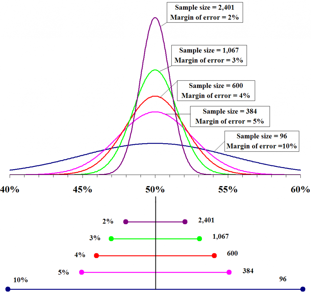
Probability densities of polls of different sizes, each color-coded to its 95% confidence interval (below), margin of error (left), and sample size (right). Each interval reflects the range within which one may have 95% confidence that the true percentage may be found, given a reported percentage of 50%. The margin of error is half the confidence interval (also, the radius of the interval). The larger the sample, the smaller the margin of error. Also, the further from 50% the reported percentage, the smaller the margin of error.
The margin of error is a statistic expressing the amount of random sampling error in the results of a survey. The larger the margin of error, the less confidence one should have that a poll result would reflect the result of a census of the entire population. The margin of error will be positive whenever a population is incompletely sampled and the outcome measure has positive variance, which is to say, the measure varies.
The term margin of error is often used in non-survey contexts to indicate observational error in reporting measured quantities.
Concept[edit]
Consider a simple yes/no poll  as a sample of
  respondents drawn from a population
  reporting the percentage
  of yes responses. We would like to know how close is to the true result of a survey of the entire population
  , without having to conduct one. If, hypothetically, we were to conduct poll over subsequent samples of respondents (newly drawn from ), we would expect those subsequent results
  to be normally distributed about
  . The margin of error describes the distance within which a specified percentage of these results is expected to vary from .
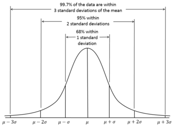
According to the 68-95-99.7 rule, we would expect that 95% of the results will fall within about two standard deviations ( ) either side of the true mean . This interval is called the confidence interval, and the radius (half the interval) is called the margin of error, corresponding to a 95% confidence level.
Generally, at a confidence level  , a sample sized of a population having expected standard deviation
  has a margin of error

where  denotes the quantile (also, commonly, a z-score), and
  is the standard error.
Standard deviation and standard error[edit]
We would expect the normally distributed values to have a standard deviation which somehow varies with . The smaller , the wider the margin. This is called the standard error  .
.
For the single result from our survey, we assume that  , and that all subsequent results together would have a variance
  .
.

Note that  corresponds to the variance of a Bernoulli distribution.
Maximum margin of error at different confidence levels[edit]
For a confidence level , there is a corresponding confidence interval about the mean  , that is, the interval
 ![{displaystyle [mu -z_{gamma }sigma ,mu +z_{gamma }sigma ]}](https://wikimedia.org/api/rest_v1/media/math/render/svg/a4568060e0cffbc8dfb793aa2ef4617c89cb9e94) within which values of should fall with probability . Precise values of are given by the quantile function of the normal distribution (which the 68-95-99.7 rule approximates).
within which values of should fall with probability . Precise values of are given by the quantile function of the normal distribution (which the 68-95-99.7 rule approximates).
Note that is undefined for  , that is,
  is undefined, as is
  .
.
|
|
|
|
|
|
|---|---|---|---|---|
| 0.68 | 0.994457883210 | 0.999 | 3.290526731492 | |
| 0.90 | 1.644853626951 | 0.9999 | 3.890591886413 | |
| 0.95 | 1.959963984540 | 0.99999 | 4.417173413469 | |
| 0.98 | 2.326347874041 | 0.999999 | 4.891638475699 | |
| 0.99 | 2.575829303549 | 0.9999999 | 5.326723886384 | |
| 0.995 | 2.807033768344 | 0.99999999 | 5.730728868236 | |
| 0.997 | 2.967737925342 | 0.999999999 | 6.109410204869 |

Since  at
at  , we can arbitrarily set
  , calculate
  , , and
  to obtain the maximum margin of error for at a given confidence level and sample size , even before having actual results. With


Also, usefully, for any reported 

Specific margins of error[edit]
If a poll has multiple percentage results (for example, a poll measuring a single multiple-choice preference), the result closest to 50% will have the highest margin of error. Typically, it is this number that is reported as the margin of error for the entire poll. Imagine poll reports  as
as 
 (as in the figure above)


As a given percentage approaches the extremes of 0% or 100%, its margin of error approaches ±0%.
Comparing percentages[edit]
Imagine multiple-choice poll reports as  . As described above, the margin of error reported for the poll would typically be
  , as
, as  is closest to 50%. The popular notion of statistical tie or statistical dead heat, however, concerns itself not with the accuracy of the individual results, but with that of the ranking of the results. Which is in first?
If, hypothetically, we were to conduct poll over subsequent samples of respondents (newly drawn from ), and report result  , we could use the standard error of difference to understand how
  is expected to fall about
  . For this, we need to apply the sum of variances to obtain a new variance,
  ,
,

where  is the covariance of
  and
and  .
.
Thus (after simplifying),


Note that this assumes that  is close to constant, that is, respondents choosing either A or B would almost never chose C (making and close to perfectly negatively correlated). With three or more choices in closer contention, choosing a correct formula for becomes more complicated.
Effect of finite population size[edit]
The formulae above for the margin of error assume that there is an infinitely large population and thus do not depend on the size of population , but only on the sample size . According to sampling theory, this assumption is reasonable when the sampling fraction is small. The margin of error for a particular sampling method is essentially the same regardless of whether the population of interest is the size of a school, city, state, or country, as long as the sampling fraction is small.
In cases where the sampling fraction is larger (in practice, greater than 5%), analysts might adjust the margin of error using a finite population correction to account for the added precision gained by sampling a much larger percentage of the population. FPC can be calculated using the formula[1]

…and so, if poll were conducted over 24% of, say, an electorate of 300,000 voters,


Intuitively, for appropriately large ,


In the former case, is so small as to require no correction. In the latter case, the poll effectively becomes a census and sampling error becomes moot.
See also[edit]
- Engineering tolerance
- Key relevance
- Measurement uncertainty
- Random error
References[edit]
- ^ Isserlis, L. (1918). «On the value of a mean as calculated from a sample». Journal of the Royal Statistical Society. Blackwell Publishing. 81 (1): 75–81. doi:10.2307/2340569. JSTOR 2340569. (Equation 1)
Sources[edit]
- Sudman, Seymour and Bradburn, Norman (1982). Asking Questions: A Practical Guide to Questionnaire Design. San Francisco: Jossey Bass. ISBN 0-87589-546-8
- Wonnacott, T.H.; R.J. Wonnacott (1990). Introductory Statistics (5th ed.). Wiley. ISBN 0-471-61518-8.
External links[edit]
- «Errors, theory of», Encyclopedia of Mathematics, EMS Press, 2001 [1994]
- Weisstein, Eric W. «Margin of Error». MathWorld.
Introduction
While you are learning statistics, you will often have to focus on a sample rather than the entire population. This is because it is extremely costly, difficult and time-consuming to study the entire population. The best you can do is to take a random sample from the population – a sample that is a ‘true’ representative of it. You then carry out some analysis using the sample and make inferences about the population.
Since the inferences are made about the population by studying the sample taken, the results cannot be entirely accurate. The degree of accuracy depends on the sample taken – how the sample was selected, what the sample size is, and other concerns. Common sense would say that if you increase the sample size, the chances of error will be less because you are taking a greater proportion of the population. A larger sample is likely to be a closer representative of the population than a smaller one.
Let’s consider an example. Suppose you want to study the scores obtained in an examination by students in your college. It may be time-consuming for you to study the entire population, i.e. all students in your college. Hence, you take out a sample of, say, 100 students and find out the average scores of those 100 students. This is the sample mean. Now, when you use this sample mean to infer about the population mean, you won’t be able to get the exact population means. There will be some “margin of error”.
You will now learn the answers to some important questions: What is margin of error, what are the method of calculating margins of error, how do you find the critical value, and how to decide on t-score vs z-scores. Thereafter, you’ll be given some margin of error practice problems to make the concepts clearer.
What is Margin of Error?
The margin of error can best be described as the range of values on both sides (above and below) the sample statistic. For example, if the sample average scores of students are 80 and you make a statement that the average scores of students are 80 ± 5, then here 5 is the margin of error.
Calculating Margins of Error
For calculating margins of error, you need to know the critical value and sample standard error. This is because it’s calculated using those two pieces of information.
The formula goes like this:
margin of error = critical value * sample standard error.
How do you find the critical value, and how to calculate the sample standard error? Below, we’ll discuss how to get these two important values.
How do You find the Critical Value?
For finding critical value, you need to know the distribution and the confidence level. For example, suppose you are looking at the sampling distribution of the means. Here are some guidelines.
- If the population standard deviation is known, use z distribution.
- If the population standard deviation is not known, use t distribution where degrees of freedom = n-1 (n is the sample size). Note that for other sampling distributions, degrees of freedom can be different and should be calculated differently using appropriate formula.
- If the sample size is large, then use z distribution (following the logic of Central Limit Theorem).
It is important to know the distribution to decide what to use – t-scores vs z-scores.
Caution – when your sample size is large and it is not given that the distribution is normal, then by Central Limit Theorem, you can say that the distribution is normal and use z-score. However, when the sample size is small and it is not given that the distribution is normal, then you cannot conclude anything about the normality of the distribution and neither z-score nor t-score can be used.
When finding the critical value, confidence level will be given to you. If you are creating a 90% confidence interval, then confidence level is 90%, for 95% confidence interval, the confidence level is 95%, and so on.
Here are the steps for finding critical value:
Step 1: First, find alpha (the level of significance). alpha =1 – Confidence level.
For 95% confidence level, alpha =0.05
For 99% confidence level, alpha =0.01
Step 2: Find the critical probability p*. Critical probability will depend on whether we are creating a one-sided confidence interval or a two-sided confidence interval.
For two-sided confidence interval, p*=1-dfrac { alpha }{ 2 }
For one-sided confidence interval, p*=1-alpha
Then you need to decide on using t-scores vs z-scores. Find a z-score having a cumulative probability of p*. For a t-statistic, find a t-score having a cumulative probability of p* and the calculated degrees of freedom. This will be the critical value. To find these critical values, you should use a calculator or respective statistical tables.
Sample Standard Error
Sample standard error can be calculated using population standard deviation or sample standard deviation (if population standard deviation is not known). For sampling distribution of means:
Let sample standard deviation be denoted by s, population standard deviation is denoted by sigma and sample size be denoted by n.
text {Sample standard error}=dfrac { sigma }{ sqrt { n } }, if sigma is known
text {Sample standard error}=dfrac { s }{ sqrt { n } }, if sigma is not known
Depending on the sampling distributions, the sample standard error can be different.
Having looked at everything that is required to create the margin of error, you can now directly calculate a margin of error using the formula we showed you earlier:
Margin of error = critical value * sample standard error.
Some Relationships
1. Confidence level and marginal of error
As the confidence level increases, the critical value increases and hence the margin of error increases. This is intuitive; the price paid for higher confidence level is that the margin of errors increases. If this was not so, and if higher confidence level meant lower margin of errors, nobody would choose a lower confidence level. There are always trade-offs!
2. Sample standard deviation and margin of error
Sample standard deviation talks about the variability in the sample. The more variability in the sample, the higher the chances of error, the greater the sample standard error and margin of error.
3. Sample size and margin of error
This was discussed in the Introduction section. It is intuitive that a greater sample size will be a closer representative of the population than a smaller sample size. Hence, the larger the sample size, the smaller the sample standard error and therefore the smaller the margin of error.
Margin of Error Practice Problems
Example 1
25 students in their final year were selected at random from a high school for a survey. Among the survey participants, it was found that the average GPA (Grade Point Average) was 2.9 and the standard deviation of GPA was 0.5. What is the margin of error, assuming 95% confidence level? Give correct interpretation.
Step 1: Identify the sample statistic.
Since you need to find the confidence interval for the population mean, the sample statistic is the sample mean which is the average GPA = 2.9.
Step 2: Identify the distribution – t, z, etc. – and find the critical value based on whether you need a one-sided confidence interval or a two-sided confidence interval.
Since population standard deviation is not known and the sample size is small, use a t distribution.
text {Degrees of freedom}=n-1=25-1=24.
alpha=1-text {Confidence level}=1-0.95=0.05
Let the critical probability be p*.
For two-sided confidence interval,
p*=1-dfrac { alpha }{ 2 } =1-dfrac { 0.05 }{ 2 } =0.975.
The critical t value for cumulative probability of 0.975 and 24 degrees of freedom is 2.064.
Step 3: Find the sample standard error.
text{Sample standard error}=dfrac { s }{ sqrt { n } } =dfrac { 0.5 }{ sqrt { 25 } } =0.1
Step 4: Find margin of error using the formula:
Margin of error = critical value * sample standard error
= 2.064 * 0.1 = 0.2064
Interpretation: For a 95% confidence level, the average GPA is going to be 0.2064 points above and below the sample average GPA of 2.9.
Example 2
400 students in Princeton University are randomly selected for a survey which is aimed at finding out the average time students spend in the library in a day. Among the survey participants, it was found that the average time spent in the university library was 45 minutes and the standard deviation was 10 minutes. Assuming 99% confidence level, find the margin of error and give the correct interpretation of it.
Step 1: Identify the sample statistic.
Since you need to find the confidence interval for the population mean, the sample statistic is the sample mean which is the mean time spent in the university library = 45 minutes.
Step 2: Identify the distribution – t, z, etc. and find the critical value based on whether the need is a one-sided confidence interval or a two-sided confidence interval.
The population standard deviation is not known, but the sample size is large. Therefore, use a z (standard normal) distribution.
alpha=1-text{Confidence level}=1-0.99=0.01
Let the critical probability be p*.
For two-sided confidence interval,
p*=1-dfrac { alpha }{ 2 } =1-dfrac { 0.01 }{ 2 } =0.995.
The critical z value for cumulative probability of 0.995 (as found from the z tables) is 2.576.
Step 3: Find the sample standard error.
text{Sample standard error}=dfrac { s }{ sqrt { n } } =dfrac { 10 }{ sqrt { 400 } } =0.5
Step 4: Find margin of error using the formula:
Margin of error = critical value * sample standard error
= 2.576 * 0.5 = 1.288
Interpretation: For a 99% confidence level, the mean time spent in the library is going to be 1.288 minutes above and below the sample mean time spent in the library of 45 minutes.
Example 3
Consider a similar set up in Example 1 with slight changes. You randomly select X students in their final year from a high school for a survey. Among the survey participants, it was found that the average GPA (Grade Point Average) was 3.1 and the standard deviation of GPA was 0.7. What should be the value of X (in other words, how many students you should select for the survey) if you want the margin of error to be at most 0.1? Assume 95% confidence level and normal distribution.
Step 1: Find the critical value.
alpha=1-text{Confidence level}=1-0.95=0.05
Let the critical probability be p*.
For two-sided confidence interval,
p*=1-dfrac { alpha }{ 2 } =1-dfrac { 0.05 }{ 2 } =0.975.
The critical z value for cumulative probability of 0.975 is 1.96.
Step 3: Find the sample standard error in terms of X.
text{Sample standard error}=dfrac { s }{ sqrt { X } }=dfrac { 0.7 }{ sqrt { X } }
Step 4: Find X using margin of error formula:
Margin of error = critical value * sample standard error
0.1=1.96*dfrac { 0.7 }{ sqrt { X } }
This gives X=188.24.
Thus, a sample of 189 students should be taken so that the margin of error is at most 0.1.
Conclusion
The margin of error is an extremely important concept in statistics. This is because it is difficult to study the entire population and the sampling is not free from sampling errors. The margin of error is used to create confidence intervals, and most of the time the results are reported in the form of a confidence interval for a population parameter rather than just a single value. In this article, you made a beginning by learning answering questions like what is margin of error, what is the method of calculating margins of errors, and how to interpret these calculations. You also learned to decide whether to use t-scores vs z-scores and gained information about finding critical values. Now you know how to use margin of error for constructing confidence intervals, which are widely used in statistics and econometrics.
Let’s put everything into practice. Try this Statistics practice question:

Looking for more Statistics practice?
You can find thousands of practice questions on Albert.io. Albert.io lets you customize your learning experience to target practice where you need the most help. We’ll give you challenging practice questions to help you achieve mastery in Statistics.
Start practicing here.
Are you a teacher or administrator interested in boosting Statistics student outcomes?
Learn more about our school licenses here.
As discussed in the previous section, the margin of error for sample estimates will shrink with the square root of the sample size. For example, a typical margin of error for sample percents for different sample sizes is given in Table 2.1 and plotted in Figure 2.2.
Numbers used to Summarize Measurement Data
| Sample Size (n) | Margin of Error (M.E.) |
|---|---|
| 200 | 7.1% |
| 400 | 5.0% |
| 700 | 3.8% |
| 1000 | 3.2% |
| 1200 | 2.9% |
| 1500 | 2.6% |
| 2000 | 2.2% |
| 3000 | 1.8% |
| 4000 | 1.6% |
| 5000 | 1.4% |
Let’s look at the implications of this square root relationship. To cut the margin of error in half, like from 3.2% down to 1.6%, you need four times as big of a sample, like going from 1000 to 4000 respondents. To cut the margin of error by a factor of five, you need 25 times as big of a sample, like having the margin of error go from 7.1% down to 1.4% when the sample size moves from n = 200 up to n = 5000.XXXXXXXXXXXXXXXXXXXXXX
Margin of Error (M.E.)
Sample size (n)
0
1000
1.00%
2.00%
3.00%
4.00%
5.00%
6.00%
7.00%
2000
3000
4000
5000
Figure 2.2 Relationship Between Sample Size and Margin of Error
In Figure 2.2, you again find that as the sample size increases, the margin of error decreases. However, you should also notice that there is a diminishing return from taking larger and larger samples. in the table and graph, the amount by which the margin of error decreases is most substantial between samples sizes of 200 and 1500. This implies that the reliability of the estimate is more strongly affected by the size of the sample in that range. In contrast, the margin of error does not substantially decrease at sample sizes above 1500 (since it is already below 3%). It is rarely worth it for pollsters to spend additional time and money to bring the margin of error down below 3% or so. After that point, it is probably better to spend additional resources on reducing sources of bias that might be on the same order as the margin of error. An obvious exception would be in a government survey, like the one used to estimate the unemployment rate, where even tenths of a percent matter.
What is a sampling error?
A sampling error occurs when the sample used in the study is not representative of the whole population. Sampling errors often occur, and thus, researchers always calculate a margin of error during final results as a statistical practice. The margin of error is the amount of error allowed for a miscalculation to represent the difference between the sample and the actual population.
Select your respondents
What are the most common sampling errors in market research?
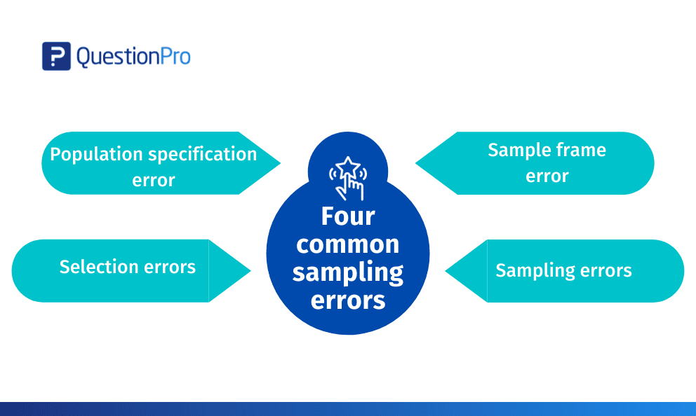
Here are the top four market research errors while sampling:
- Population specification error: A population specification error occurs when researchers don’t know precisely who to survey. For example, imagine a research study about kid’s apparel. Who is the right person to survey? It can be both parents, only the mother, or the child. The parents make purchase decisions, but the kids may influence their choice.
- Sample frame error: Sampling frame errors arise when researchers target the sub-population wrongly while selecting the sample. For example, picking a sampling frame from the telephone white pages book may have erroneous inclusions because people shift their cities. Erroneous exclusions occur when people prefer to un-list their numbers. Wealthy households may have more than one connection, thus leading to multiple inclusions.
- Selection error: A selection error occurs when respondents self-select themselves to participate in the study. Only the interested ones respond. You can control selection errors by going the extra step to request responses from the entire sample. Pre-survey planning, follow-ups, and a neat and clean survey design will boost respondents’ participation rate. Also, try methods like CATI surveys and in-person interviews to maximize responses.
- Sampling errors: Sampling errors occur due to a disparity in the representativeness of the respondents. It majorly happens when the researcher does not plan his sample carefully. These sampling errors can be controlled and eliminated by creating a careful sample design, having a large enough sample to reflect the entire population, or using an online sample or survey audiences to collect responses.
Controlling your sampling error
Statistical theories help researchers measure the probability of sampling errors in sample size and population. The size of the sample considered from the population primarily determines the size of the sampling error. Larger sample sizes tend to encounter a lower rate of errors. Researchers use a metric known as the margin of error to understand and evaluate the margin of error. Usually, a confidence level of 95% is considered to be the desired confidence level.
Pro Tip: If you need help calculating your own margin of error, you can use our Margin of Error Calculator.
What are the steps to reduce sampling errors?
Sampling errors are easy to identify. Here are a few simple steps to reduce sampling error:
- Increase sample size: A larger sample size results in a more accurate result because the study gets closer to the actual population size.
- Divide the population into groups: Test groups according to their size in the population instead of a random sample. For example, if people of a specific demographic make up 20% of the population, make sure that your study is made up of this variable to reduce sampling bias.
- Know your population: Study your population and understand its demographic mix. Know what demographics use your product and service and ensure you only target the sample that matters.
We have also created a tool to help you determine your sample easily: Sample Size Calculator.
A sampling error is measurable, and researchers can use it to their advantage to estimate the accuracy of their findings and estimate variance.
What does sampling error mean?
A sampling error is a type of error that happens when the sample used in particular research is unable to represent the entire population. These types of errors occur quite often, so, researchers have adopted a statistical practice of calculating a margin of error at the time of final results. The margin of error covers the total amount of miscalculation error that indicates the difference between a specific sample and the actual population size.
What are the types of sampling errors in market research?
There are four types of market research errors that usually occur while sampling:

Population specification error: This is the type of error that happens when researchers aren’t aware of who to survey actually. For instance, an apparel brand is planning to launch a new summer collection for kids. In this case, who should be surveyed? The child or the parents? While the purchasing power lies in the hands of parents, kids can completely influence their decision.
Sample frame error: A sample frame error occurs when a researcher targets the wrong sub-population at the time of selecting a sample. For instance, choosing a sampling frame from a particular telephone directory might have erroneous inclusions as people keep changing their location (majorly cities). Also, when people start un-listing their numbers, that’s when erroneous exclusions mainly occur. In fact, financially strong and wealthy people usually have more than one connection, which leads to numerous inclusions.
Selection error: Selection errors are the types of errors that happen when respondents are given the authority to self-select themselves for participating in the research. In this case, you get responses only from the interested candidates. To efficiently control selection errors, you need to put in extra effort by requesting responses from the entire sample set. With effective pre-survey planning, continuous follow-ups, and clear survey design, you can effortlessly increase the participation rate of the respondents. Also, leveraging CATI surveys and face-to-face interviews is a great way of maximizing responses.
Sampling errors: Sampling errors are a result of disparity that occurs in representing a group of respondents. It usually happens in case of improper sample planning, i.e. when a researcher fails to plan his sample accurately. These types of errors can be eliminated by developing an effective sample design, creating a large sample size that reflects the whole population, or leveraging an online sample for collecting responses.
[Free Webinar Recording]
Want to know how to increase your survey response rates?
Learn how to meet respondents where they are, drive survey completion while offering a seamless experience, Every Time!
How to control sampling error?
Statistical theories are considered to be effective in measuring the probability of sampling errors and most researchers rely on them for controlling the errors in their sample size and population. The size of the sampling error usually relies on the sample size considered by the researcher. While larger sample sizes are known to experience fewer errors, smaller sample sizes may encounter a higher rate of errors. To seamlessly understand as well as evaluate the range of error, researchers use a metric that is popularly known as “margin of error”. Majorly, a confidence level of 95% is desired by every researcher.
What are the steps involved in reducing sampling errors?
The process of identifying sampling errors is easy and so is their reduction. Here’s how you can reduce sampling errors:
By increasing sample size: Using a larger sample size helps to yield more effective and accurate results as the research becomes closer to the true population size.
By creating groups to segment the population: Instead of choosing a random sample, create and test groups based on their size in the population. For instance, if people of a certain demographic constitute 30% of the total population, it’s important to ensure that your research is based on this variable.
By knowing your population well: To reduce sampling errors, it’s essential to understand your population and be aware of its demographic mix. Delve deeper to uncover the demographics that use your product or service and always target the right sample (that actually matters to your business).
As sampling error can be measured, most of the researchers use it for gaining a competitive advantage and estimating the accuracy & effectiveness of their findings in market research.
Most of the students are not aware of the types of error in statistics. This guide will help you to know everything about the types of error in statistics. Let’s explore the guide:-
As ‘statistics’ relates to the mathematical term, individuals start analyzing it as a problematic terminology, but it is the most exciting and straightforward form of mathematics.
As the word ‘statistics’ refers that it consists of quantified statistic figures. That we use to represent and summarize the given data of an experiment or the real-time studies. In this article, we will discuss the following topics in detail:-
- What is the error in statistics?
- What is the standard error in statistics?
- How many types of errors in statistics?
- What are the sampling error and non-sampling error in statistics?
- What is the margin of error in statistics formula?
Before discussing these topics as mentioned above in this article, we want to say that you can find any statistics assignment from our experts on ‘statistics homework help.’
What is the error in statistics?
Statistics is a methodology of gathering, analyzing, reviewing, and drawing the particular information’s conclusion. The statistical error is the difference between the collected data’s obtained value and the actual value of the collected data. The higher the error value, the lesser will be the representative data of the community.
In simple words, a statistics error is a difference between a measured value and the actual value of the collected data. If the error value is more significant, then the data will be considered as the less reliable. Therefore, one has to keep in mind that the data must have minimal error value. So that the data can be considered to be more reliable.
There are two types of error in statistics that is the type I & type II. In a statistical test, the Type I error is the elimination of the true null theories. In contrast, the type II error is the non-elimination of the false null hypothesis.
Plenty of the statistical method rotates around the reduction of one or both kind of errors, although the complete rejection of either of them is impossible.
But by choosing the low threshold value and changing the alpha level, the features of the hypothesis test could be maximized. The information on type I error & type II error is used for bio-metrics, medical science, and computer science.
Type I error
The initial type of error is eliminating a valid null hypothesis, which is considered the outcome of a test procedure. This type of error is sometimes also called an error of the initial type/kind.
A null hypothesis is set before the beginning of an analysis. But for some situations, the null hypothesis is considered as not being present in the ‘cause and effect’ relationship of the items that are being tested.
This situation is donated as ‘n=0’ if you are conducting the test, and the outcome seems to signify that applied stimuli may cause a response, then the null hypothesis will be rejected.
Examples of type I error
Let’s take an example of the trail of a condemned criminal. The null hypothesis can be considered as an innocent person, while others treat it as guilty. In this case, Type I error means that the individual is not found to be innocent. And individual needs to be sent to jail, despite being an innocent.
In another example, in medicinal tests, a Type I would bring its display as a cure of disease tends to minimize the seriousness of a disease, but actually, it is not doing the same.
Whenever a new dose of disease is tested, then the null hypothesis would consider as the dose will not disturb the progress of the particular ailment. Let’s take an example of it as a lab research a new cancer dose. The null hypothesis would be that the dose will not disturb the progress of the cancer cells.
After treating the cancer cells with medicine, the cancer cells will not progress. This may result to eliminate the null hypothesis of that drug that does not have any effect. The medicine is successful in stopping the growth of cancer cells, then the conclusion of rejecting the null value will be correct.
However, while testing the medicine, something else would help to stop the growth rather than the medicine, then this could be treated as an example of an incorrect elimination of the null hypothesis that is a type I error.
Type II error
A type II error implies the non-elimination of a wrong null hypothesis. We use this kind of error for the text of hypothesis testing. In the statistical data analysis, type I errors are the elimination of the true null hypothesis.
On the other hand, type II error is a kind of error that happens when someone is not able to eliminate a null hypothesis, which is wrong. In simple words, type II error generates a false positive. The error eliminates the other hypothesis, even though that does not happen due to chance.
A type II error proves an idea that has been eliminated, demanding the two observances could be identical, even though both of them are dissimilar. Besides, a type II errors do not eliminate the null hypothesis. Even though the other hypothesis has the true nature, or wrre can say that a false value is treated as true. A type II error is well-known as a ‘beta error’.
Type II Error’s example
Suppose a biometric company likes to compare the effectivity of the two medicines that are used for treating diabetic patients. The null hypothesis refers to the two treatments that are of similar effectivity.
A null hypothesis (H) is the demand of the organization that concern to eliminate one-tailed test uses. The other hypothesis refers to the two medications are not identically effective. The other hypothesis (Ha) is the calculation, which is backed by eliminating the null hypothesis.
The biotechnical organization decided to conduct a test on 4,000 diabetic patients to evaluate the treating effectivity. The organization anticipates the two medicines should have a similar number of diabetic patients to ensure the effectivity of the drugs. It chooses a significant value of 0.05 that signifies that it is ready to adopt a 6% chance of eliminating the null hypothesis when it is considered to be real or a chance of 6% of carrying out a type I error.
Suppose beta would be measured as 0.035 or as 3.5%. So, the chances of carrying out a type II error is 3.5%. When the two cures are not identical, then the null hypothesis must be eliminated. Still, the biotechnical organization does not eliminate the null hypothesis if the medicine is not identically effective, then the type II error happens.
Test your knowledge about types of error in statistics
- A Type I error occurs if
- A null hypothesis needs to be not rejected but must be rejected.
- The given null hypothesis is rejected, but actually, it needs not be rejected.
- A test statistic is wrong.
- None of these.
Correct Answer: The given null hypothesis is rejected, but actually, it needs not be rejected.
2. A Type II error occurs if
- A null hypothesis needs to be not rejected but must be rejected.
- The given null hypothesis is rejected, but actually, it needs not be rejected.
- A test statistic is wrong.
- None of these.
Correct Answer: A null hypothesis needs to be not rejected but must be rejected.
3. Deciding on the significance level ‘α’ helps in determining
- the Type II error’s probability.
- the Type I error’s probability.
- the power.
- None of these.
Correct Answer: the Type I error’s probability.
4. Suppose a water bottle has a label stating – the volume is 12 oz. A user group found that the bottle is under‐filled and decided to perform a test. In this case, a Type I error would mean
- The user group does not summarize that the bottle has less than 12 oz. The mean is also less than 12 oz.
- The user group has proof that the label is wrong.
- The user group summarizes that the bottle has less than 12 oz. The mean is also 12 oz.
- None of these.
Correct Answer: The user group summarizes that the bottle has less than 12 oz. The mean is also 12 oz.
5. A Type I error happens in the case the null hypothesis is
- correct.
- incorrect.
- either correct or incorrect.
- None of these.
Correct Answer: correct.
6. A Type II error happens in the case the null hypothesis is
- correct.
- incorrect.
- either correct or incorrect.
- None of these.
Correct Answer: incorrect.
7. Suppose the significance level ‘α’ is raised; in this case, the uncertainty of a Type I error will also
- decrease.
- remain the same.
- increase.
- None of these.
Correct Answer: increase.
8. Suppose the significance level ‘α’ is raised; in this case, the uncertainty of a Type II error will also
- decrease.
- remain the same.
- increase.
- None of these.
Correct Answer: decrease.
9. Suppose the significance level ‘α’ is raised; in this case, the power will also
- decrease.
- remain the same.
- increase.
- None of these.
Correct Answer: increase.
10. The test’s power can increase by
- selecting a smaller value for α.
- using a normal approximation.
- using a larger sample size.
- None of these.
Correct Answer: using a larger sample size.
What is the standard error in statistics?
‘Standard error’ refers to the standard deviation of several statistics samples, like mean and median. For instance, the term “standard error in statistics” would refer to as the standard deviation of the given distributing data that is calculated from a population. The smaller the value of the standard error, the larger representative the overall data.
The relation between standard deviation and the standard error is that for a provided data, the standard error is equal to the standard deviation (SD) upon the square root of the offered data size.
Standard error = standard deviation
√ Given data
The standard error is inversely proportional to the given model size, which means the higher the model size, the lesser the value of standard error since the statistic will tend to the actual value.
Standard error ∝ 1/sample size
The standard error is taken as a portion of explanatory statistics. The standard error shows the standard deviation (SD) of an average value into a data set. It treats as a calculation of the random variables as well as to the extent. The smaller the extent, the higher the accuracy of the dataset.
The data affects two kinds of error
Sampling error
Sampling error happens only as an outcome of using a model from a population instead of than conducting a complete enumeration of the population. It implies a difference between a prediction of the value of community and the ‘true or real’ value of that sample population that would result if a census would be taken. The sampling error does not happen in a census as it is based on the whole community.
Sampling error would cause when:
- The method of sampling is not accidental.
- The samples are smaller to show the population accurately.
- The proportions of several features within the sample would not be identical to the proportion of the features for the entire population.
Sampling error can be calculated and handled in random samples. Especially where every unit has a hope of selection, and the hope can be measured. In other words, the increment in the sample size would decrements in the sampling error.
2. Non-sampling error
This error is caused by other factors that are not associated with the sample selection. It implies the existence of any of the factors, whether a random or systematic, that output as the true value of the population. The non-sampling error can happen at any step of a census or study sample. And it is not easily quantified or identified.
Non-sampling error can consist
- Non-reaction error: This mention the failure to get a response from a few units since of absence, refusal, non-contact, or some other reason. The non-reaction error can be a partial reaction (that is, a chosen unit has not supported the solution to a few problems) or a complete reaction (that is no information has been taken at all from a chosen unit).
- Processing error: It implies the error found during the process of collecting the data, coding, data entry, editing, and outputting.
- Coverage error: This happens when a unit of the sample is not correctly included or excluded or is replicated in the sample (for example, an interviewer is not able to interview a chosen household).
- Interviewer error: This error happens when the interviewer record a piece of information incorrectly, is not objective or neutral or assumes reaction based on looks or other features.
What is the margin of error in statistics?
The margin of error in statistics is the order of the values above and below the samples in a given interval. The given range is a method to represent what the suspicious is with a particular statistic.
For example, a survey may be referred that there is a 97% confidence interval of 3.88 and 4.89. This means that when a survey would be conducted again with the same technical method, 97% of the time, the real population statistic will lay within the estimated interval (i.e., 3.88 and 4.89) 97% of the time.
The formula for calculating the margin of error percentage
A marginal error implies to you how many different values would be resulted from the true population value. For instance, a 94% confidence interval by a 3% margin of error means that your calculated statistics would be within 3% points to the true population value 945 of the time.
The Margin of Error can be measured in two ways:
- The margin of error = Standard deviation of the statistics x Critical range value
- The margin of error = Standard error of the statistic x Critical value
Steps on Calculate Margin of Error
Step 1: Calculate the critical value. The critical value is either of a z-score or t-score. In general, for the smaller value (under 30) or when you do not have the standard deviation of the population. Then use a t-score, in another way, use a z-score.
Step 2: Calculate the standard error or standard deviation. These two are an identical thing, and merely you should have the population parameter value to measure standard deviation.
Step 3: Multiply the standard deviation and the critical value.
Sample problem: 100 students were polled and had a GPA of 2.5 with a standard deviation of 0.5. Calculate the margin of error in statistics for a 90% confidence range.
- The value of critical for a 90% confidence range is 1.645 (see the table of z-score).
- The SD is 0.5 (as it is a sample, we require the standard error for the mean.) the SE can be calculated as the standard deviation / √ Given data; therefore, 0.5/ √ (100) = 0.05.
- 1.645*0.05 = 0.08125.
The margin of error for a proportion formula:
where :
p-hat = sample proportion; n= sample size; z= z-score
Steps to calculate margin error for a proportion
Step 1: Calculate p-hat. This can be calculated by the number of the population who have been responded positively. It means that they have given the answer related to the given statement of the question.
Step 2: Calculate the z-score with follows the confidence level value.
Step3: Put all the value in the given formula:
Step 4: Convert step 3 into the percentage.
Sample problem
1000 individuals were polled, and 380 think that climate alters not because of human pollution. Calculate the ME for a given 90% confidence value.
- The number of individuals who respond positively; 38%.
- A 90% confidence level has a critical value (z-score) of 1.645.
- Calculate the value by using the formula
=1.645*[ √ {(38*.62)/(1000)}]
=0.0252
4. Convert the value into a percentage.
0.0252= 2.52%
The margin of error in statistics is 2.52%.
Conclusion
This is all about types of error in statistics. Use the details as mentioned earlier, you can understand types of error in statistics. But, still, you find any issue related to the topic error in statistics. Then you can get in touch 24*7 with our professional experts. They have enough knowledge of this particular topic; therefore, they can resolve all the queries of yours.
Get the best statistics homework help from the professional experts at a reasonable price. We provide you the assignment before the deadline so that you can check your work. And we also provide a plagiarism-free report which defines the uniqueness of the content. We are providing world-class help on math assignment help to the students who are living across the globe. We are the most reliable math assignment helpers in the world.
Frequently Asked Question
What is the difference between Type 1 and Type 2 errors?
In statistical hypothesis testing, Type 1 error is caused by rejecting any of the null hypotheses (in case it has true value). Type II error occurs while a null hypothesis is taken (if it does not have a true value).
What is random error example?
A random error can happen because of the measuring instrument and can be affected by variations in the experimental environment. For example, a spring balance can produce some variation in calculations because of the unloading and loading conditions, fluctuations in temperature, etc.
What type of error is human error?
Random errors are considered to be natural errors. Systematic errors occur because of problems or imprecision with instruments. Now, human error is something that humans screwed up; they have made a mistake. These cause human errors.