Hamming code is a block code that is capable of detecting up to two simultaneous bit errors and correcting single-bit errors. It was developed by R.W. Hamming for error correction.
In this coding method, the source encodes the message by inserting redundant bits within the message. These redundant bits are extra bits that are generated and inserted at specific positions in the message itself to enable error detection and correction. When the destination receives this message, it performs recalculations to detect errors and find the bit position that has error.
Hamming Code for Single Error Correction
The procedure for single error correction by Hamming Code includes two parts, encoding at the sender’s end and decoding at receiver’s end.
Encoding a message by Hamming Code
The procedure used by the sender to encode the message encompasses the following steps −
-
Step 1 − Calculation of the number of redundant bits.
-
Step 2 − Positioning the redundant bits.
-
Step 3 − Calculating the values of each redundant bit.
Once the redundant bits are embedded within the message, this is sent to the destination.
Step 1 − Calculation of the number of redundant bits.
If the message contains m number of data bits, r number of redundant bits are added to it so that is able to indicate at least (m + r + 1) different states. Here, (m + r) indicates location of an error in each of bit positions and one additional state indicates no error. Since, r bits can indicate 2r states, 2r must be at least equal to (m + r + 1). Thus the following equation should hold −
2r ≥ 𝑚 + 𝑟 + 1
Example 1 − If the data is of 7 bits, i.e. m = 7, the minimum value of r that will satisfy the above equation is 4, (24 ≥ 7 + 4 + 1). The total number of bits in the encoded message, (m + r) = 11. This is referred as (11,4) code.
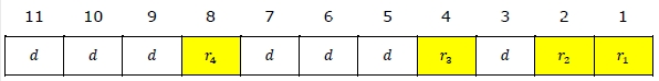
Step 2 − Positioning the redundant bits.
The r redundant bits placed at bit positions of powers of 2, i.e. 1, 2, 4, 8, 16 etc. They are referred in the rest of this text as r1 (at position 1), r2 (at position 2), r3 (at position 4), r4 (at position  and so on.
Example 2 − If, m = 7 comes to 4, the positions of the redundant bits are as follows −
Step 3 − Calculating the values of each redundant bit.
The redundant bits are parity bits. A parity bit is an extra bit that makes the number of 1s either even or odd. The two types of parity are −
-
Even Parity − Here the total number of bits in the message is made even.
-
Odd Parity − Here the total number of bits in the message is made odd.
Each redundant bit, ri, is calculated as the parity, generally even parity, based upon its bit position. It covers all bit positions whose binary representation includes a 1 in the ith position except the position of ri. Thus −
-
r1 is the parity bit for all data bits in positions whose binary representation includes a 1 in the least significant position excluding 1 (3, 5, 7, 9, 11 and so on)
-
r2 is the parity bit for all data bits in positions whose binary representation includes a 1 in the position 2 from right except 2 (3, 6, 7, 10, 11 and so on)
-
r3 is the parity bit for all data bits in positions whose binary representation includes a 1 in the position 3 from right except 4 (5-7, 12-15, 20-23 and so on)
Example 3 − Suppose that the message 1100101 needs to be encoded using even parity Hamming code. Here, m = 7 and r comes to 4. The values of redundant bits will be as follows −
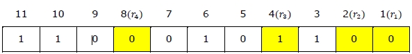
Hence, the message sent will be 11000101100.
Decoding a message in Hamming Code
Once the receiver gets an incoming message, it performs recalculations to detect errors and correct them. The steps for recalculation are −
-
Step 1 − Calculation of the number of redundant bits.
-
Step 2 − Positioning the redundant bits.
-
Step 3 − Parity checking.
-
Step 4 − Error detection and correction
Step 1) Calculation of the number of redundant bits
Using the same formula as in encoding, the number of redundant bits are ascertained.
2r ≥ 𝑚 + 𝑟 + 1
where m is the number of data bits and r is the number of redundant bits.
Step 2) Positioning the redundant bits
The r redundant bits placed at bit positions of powers of 2, i.e. 1, 2, 4, 8, 16 etc.
Step 3) Parity checking
Parity bits are calculated based upon the data bits and the redundant bits using the same rule as during generation of c1, c2, c3, c4 etc. Thus
c1 = parity(1, 3, 5, 7, 9, 11 and so on)
c2 = parity(2, 3, 6, 7, 10, 11 and so on)
c3 = parity(4-7, 12-15, 20-23 and so on)
Step 4) Error detection and correction
The decimal equivalent of the parity bits binary values is calculated. If it is 0, there is no error. Otherwise, the decimal value gives the bit position which has error. For example, if c1c2c3c4 = 1001, it implies that the data bit at position 9, decimal equivalent of 1001, has error. The bit is flipped (converted from 0 to 1 or vice versa) to get the correct message.
Example 4 − Suppose that an incoming message 11110101101 is received.
Step 1 − At first the number of redundant bits are calculated using the formula 2r ≥ m + r + 1. Here, m + r + 1 = 11 + 1 = 12. The minimum value of r such that 2r ≥ 12 is 4.
Step 2 − The redundant bits are positioned as below −
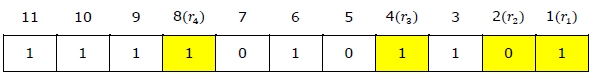
Step 3 − Even parity checking is done −
c1 = even_parity(1, 3, 5, 7, 9, 11) = 0
c2 = even_parity(2, 3, 6, 7, 10, 11) = 0
c3 = even_parity (4, 5, 6, 7) = 0
c4 = even_parity (8, 9, 10, 11) = 0
Step 4 — Since the value of the check bits c1c2c3c4 = 0000 = 0, there are no errors in this message.
Hamming Code for double error detection
The Hamming code can be modified to correct a single error and detect double errors by adding a parity bit as the MSB, which is the XOR of all other bits.
Example 5 − If we consider the codeword, 11000101100, sent as in example 3, after adding P = XOR(1,1,0,0,0,1,0,1,1,0,0) = 0, the new codeword to be sent will be 011000101100.
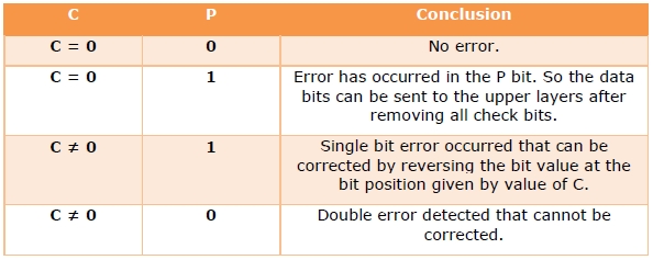
At the receiver’s end, error detection is done as shown in the following table −
A Hamming code is a particular kind of error-correcting code (ECC) that allows single-bit errors in code words to be corrected. Such codes are used in data transmission or data storage systems in which it is not feasible to use retry mechanisms to recover the data when errors are detected. This type of error recovery is also known as forward error correction (FEC).
Constructing a Hamming code to protect, say, a 4-bit data word
Hamming codes are relatively easy to construct because they’re based on parity logic. Each check bit is a parity bit for a particular subset of the data bits, and they’re arranged so that the pattern of parity errors directly indicates the position of the bit error.
It takes three check bits to protect four data bits (the reason for this will become apparent shortly), giving a total of 7 bits in the encoded word. If you number the bit positions of an 8-bit word in binary, you see that there is one position that has no «1»s in its column, three positions that have a single «1» each, and four positions that have two or more «1»s.
If the four data bits are called A, B, C and D, and our three check bits are X, Y and Z, we place them in the columns such that the check bits are in the columns with one «1» and the data bits are in the columns with more than one «1». The bit in position 0 is not used.
Bit position:  7  6  5  4  3  2  1  0
   in binary:  1  1  1  1  0  0  0  0
               1  1  0  0  1  1  0  0
               1  0  1  0  1  0  1  0
         Bit:  A  B  C  X  D  Y  Z  -
The check bit X is set or cleared so that all of the bits with a «1» in the top row — A, B C and X — have even parity. Similarly, the check bit Y is the parity bit for all of the bits with a «1» in the second row (A, B and D), and the check bit Z is the parity bit for all of the bits with a «1» in the third row (A, C and D).
Now all seven bits — the codeword — are transmitted (or stored), usually reordered so that the data bits appear in their original sequence: A B C D X Y Z. When they’re received (or retrieved) later, the data bits are put through the same encoding process as before, producing three new check bits X’, Y’ and Z’. If the new check bits are XOR’d with the received check bits, an interesting thing occurs. If there’s no error in the received bits, the result of the XOR is all zeros. But if there’s a single bit error in any of the seven received bits, the result of the XOR is a nonzero three-bit number called the «syndrome» that directly indicates the position of the bit error as defined in the table above. If the bit in this position is flipped, then the original 7-bit codeword is perfectly reconstructed.
A couple of examples will illustrate this. Let’s assume that the data bits are all zero, which also means that all of the check bits are zero as well. If bit «B» is set in the received word, then the recomputed check bits X’Y’Z’ (and the syndrome) will be 110, which is the bit position for B. If bit «Y» is set in the received word, then the recomputed check bits will be «000», and the syndrome will be «010», which is the bit position for Y.
Hamming codes get more efficient with larger codewords. Basically, you need enough check bits to enumerate all of the data bits plus the check bits plus one. Therefore, four check bits can protect up to 11 data bits, five check bits can protect up to 26 data bits, and so on. Eventually you get to the point where if you have 8 bytes of data (64 bits) with a parity bit on each byte, you have enough parity bits to do ECC on the 64 bits of data instead.
Different (but equivalent) Hamming codes
Given a specific number N of check bits, there are 2N equivalent Hamming codes that can be constructed by arbitrarily choosing each check bit to have either «even» or «odd» parity within its group of data bits. As long as the encoder and the decoder use the same definitions for the check bits, all of the properties of the Hamming code are preserved.
Sometimes it’s useful to define the check bits so that an encoded word of all-zeros or all-ones is always detected as an error.
What happens when multiple bits get flipped in a Hamming codeword
Multible bit errors in a Hamming code cause trouble. Two bit errors will always be detected as an error, but the wrong bit will get flipped by the correction logic, resulting in gibberish. If there are more than two bits in error, the received codeword may appear to be a valid one (but different from the original), which means that the error may or may not be detected.
In any case, the error-correcting logic can’t tell the difference between single bit errors and multiple bit errors, and so the corrected output can’t be relied on.
Extending a Hamming code to detect double-bit errors
Any single-error correcting Hamming code can be extended to reliably detect double bit errors by adding one more parity bit over the entire encoded word. This type of code is called a SECDED (single-error correcting, double-error detecting) code. It can always distinguish a double bit error from a single bit error, and it detects more types of multiple bit errors than a bare Hamming code does.
It works like this: All valid code words are (a minimum of) Hamming distance 3 apart. The «Hamming distance» between two words is defined as the number of bits in corresponding positions that are different. Any single-bit error is distance one from a valid word, and the correction algorithm converts the received word to the nearest valid one.
If a double error occurs, the parity of the word is not affected, but the correction algorithm still corrects the received word, which is distance two from the original valid word, but distance one from some other valid (but wrong) word. It does this by flipping one bit, which may or may not be one of the erroneous bits. Now the word has either one or three bits flipped, and the original double error is now detected by the parity checker.
Note that this works even when the parity bit itself is involved in a single-bit or double-bit error. It isn’t hard to work out all the combinations.
In computer science and telecommunication, Hamming codes are a family of linear error-correcting codes. Hamming codes can detect one-bit and two-bit errors, or correct one-bit errors without detection of uncorrected errors. By contrast, the simple parity code cannot correct errors, and can detect only an odd number of bits in error. Hamming codes are perfect codes, that is, they achieve the highest possible rate for codes with their block length and minimum distance of three.[1]Richard W. Hamming invented Hamming codes in 1950 as a way of automatically correcting errors introduced by punched card readers. In his original paper, Hamming elaborated his general idea, but specifically focused on the Hamming(7,4) code which adds three parity bits to four bits of data.[2]
| Binary Hamming codes | |
|---|---|

The Hamming(7,4) code (with r = 3) |
|
| Named after | Richard W. Hamming |
| Classification | |
| Type | Linear block code |
| Block length | 2r − 1 where r ≥ 2 |
| Message length | 2r − r − 1 |
| Rate | 1 − r/(2r − 1) |
| Distance | 3 |
| Alphabet size | 2 |
| Notation | [2r − 1, 2r − r − 1, 3]2-code |
| Properties | |
| perfect code | |
|
In mathematical terms, Hamming codes are a class of binary linear code. For each integer r ≥ 2 there is a code-word with block length n = 2r − 1 and message length k = 2r − r − 1. Hence the rate of Hamming codes is R = k / n = 1 − r / (2r − 1), which is the highest possible for codes with minimum distance of three (i.e., the minimal number of bit changes needed to go from any code word to any other code word is three) and block length 2r − 1. The parity-check matrix of a Hamming code is constructed by listing all columns of length r that are non-zero, which means that the dual code of the Hamming code is the shortened Hadamard code. The parity-check matrix has the property that any two columns are pairwise linearly independent.
Due to the limited redundancy that Hamming codes add to the data, they can only detect and correct errors when the error rate is low. This is the case in computer memory (usually RAM), where bit errors are extremely rare and Hamming codes are widely used, and a RAM with this correction system is a ECC RAM (ECC memory). In this context, an extended Hamming code having one extra parity bit is often used. Extended Hamming codes achieve a Hamming distance of four, which allows the decoder to distinguish between when at most one one-bit error occurs and when any two-bit errors occur. In this sense, extended Hamming codes are single-error correcting and double-error detecting, abbreviated as SECDED.
HistoryEdit
Richard Hamming, the inventor of Hamming codes, worked at Bell Labs in the late 1940s on the Bell Model V computer, an electromechanical relay-based machine with cycle times in seconds. Input was fed in on punched paper tape, seven-eighths of an inch wide, which had up to six holes per row. During weekdays, when errors in the relays were detected, the machine would stop and flash lights so that the operators could correct the problem. During after-hours periods and on weekends, when there were no operators, the machine simply moved on to the next job.
Hamming worked on weekends, and grew increasingly frustrated with having to restart his programs from scratch due to detected errors. In a taped interview, Hamming said, «And so I said, ‘Damn it, if the machine can detect an error, why can’t it locate the position of the error and correct it?'».[3] Over the next few years, he worked on the problem of error-correction, developing an increasingly powerful array of algorithms. In 1950, he published what is now known as Hamming code, which remains in use today in applications such as ECC memory.
Codes predating HammingEdit
A number of simple error-detecting codes were used before Hamming codes, but none were as effective as Hamming codes in the same overhead of space.
ParityEdit
Parity adds a single bit that indicates whether the number of ones (bit-positions with values of one) in the preceding data was even or odd. If an odd number of bits is changed in transmission, the message will change parity and the error can be detected at this point; however, the bit that changed may have been the parity bit itself. The most common convention is that a parity value of one indicates that there is an odd number of ones in the data, and a parity value of zero indicates that there is an even number of ones. If the number of bits changed is even, the check bit will be valid and the error will not be detected.
Moreover, parity does not indicate which bit contained the error, even when it can detect it. The data must be discarded entirely and re-transmitted from scratch. On a noisy transmission medium, a successful transmission could take a long time or may never occur. However, while the quality of parity checking is poor, since it uses only a single bit, this method results in the least overhead.
Two-out-of-five codeEdit
A two-out-of-five code is an encoding scheme which uses five bits consisting of exactly three 0s and two 1s. This provides ten possible combinations, enough to represent the digits 0–9. This scheme can detect all single bit-errors, all odd numbered bit-errors and some even numbered bit-errors (for example the flipping of both 1-bits). However it still cannot correct any of these errors.
RepetitionEdit
Another code in use at the time repeated every data bit multiple times in order to ensure that it was sent correctly. For instance, if the data bit to be sent is a 1, an n = 3 repetition code will send 111. If the three bits received are not identical, an error occurred during transmission. If the channel is clean enough, most of the time only one bit will change in each triple. Therefore, 001, 010, and 100 each correspond to a 0 bit, while 110, 101, and 011 correspond to a 1 bit, with the greater quantity of digits that are the same (‘0’ or a ‘1’) indicating what the data bit should be. A code with this ability to reconstruct the original message in the presence of errors is known as an error-correcting code. This triple repetition code is a Hamming code with m = 2, since there are two parity bits, and 22 − 2 − 1 = 1 data bit.
Such codes cannot correctly repair all errors, however. In our example, if the channel flips two bits and the receiver gets 001, the system will detect the error, but conclude that the original bit is 0, which is incorrect. If we increase the size of the bit string to four, we can detect all two-bit errors but cannot correct them (the quantity of parity bits is even); at five bits, we can both detect and correct all two-bit errors, but not all three-bit errors.
Moreover, increasing the size of the parity bit string is inefficient, reducing throughput by three times in our original case, and the efficiency drops drastically as we increase the number of times each bit is duplicated in order to detect and correct more errors.
DescriptionEdit
If more error-correcting bits are included with a message, and if those bits can be arranged such that different incorrect bits produce different error results, then bad bits could be identified. In a seven-bit message, there are seven possible single bit errors, so three error control bits could potentially specify not only that an error occurred but also which bit caused the error.
Hamming studied the existing coding schemes, including two-of-five, and generalized their concepts. To start with, he developed a nomenclature to describe the system, including the number of data bits and error-correction bits in a block. For instance, parity includes a single bit for any data word, so assuming ASCII words with seven bits, Hamming described this as an (8,7) code, with eight bits in total, of which seven are data. The repetition example would be (3,1), following the same logic. The code rate is the second number divided by the first, for our repetition example, 1/3.
Hamming also noticed the problems with flipping two or more bits, and described this as the «distance» (it is now called the Hamming distance, after him). Parity has a distance of 2, so one bit flip can be detected but not corrected, and any two bit flips will be invisible. The (3,1) repetition has a distance of 3, as three bits need to be flipped in the same triple to obtain another code word with no visible errors. It can correct one-bit errors or it can detect — but not correct — two-bit errors. A (4,1) repetition (each bit is repeated four times) has a distance of 4, so flipping three bits can be detected, but not corrected. When three bits flip in the same group there can be situations where attempting to correct will produce the wrong code word. In general, a code with distance k can detect but not correct k − 1 errors.
Hamming was interested in two problems at once: increasing the distance as much as possible, while at the same time increasing the code rate as much as possible. During the 1940s he developed several encoding schemes that were dramatic improvements on existing codes. The key to all of his systems was to have the parity bits overlap, such that they managed to check each other as well as the data.
General algorithmEdit
The following general algorithm generates a single-error correcting (SEC) code for any number of bits. The main idea is to choose the error-correcting bits such that the index-XOR (the XOR of all the bit positions containing a 1) is 0. We use positions 1, 10, 100, etc. (in binary) as the error-correcting bits, which guarantees it is possible to set the error-correcting bits so that the index-XOR of the whole message is 0. If the receiver receives a string with index-XOR 0, they can conclude there were no corruptions, and otherwise, the index-XOR indicates the index of the corrupted bit.
An algorithm can be deduced from the following description:
- Number the bits starting from 1: bit 1, 2, 3, 4, 5, 6, 7, etc.
- Write the bit numbers in binary: 1, 10, 11, 100, 101, 110, 111, etc.
- All bit positions that are powers of two (have a single 1 bit in the binary form of their position) are parity bits: 1, 2, 4, 8, etc. (1, 10, 100, 1000)
- All other bit positions, with two or more 1 bits in the binary form of their position, are data bits.
- Each data bit is included in a unique set of 2 or more parity bits, as determined by the binary form of its bit position.
- Parity bit 1 covers all bit positions which have the least significant bit set: bit 1 (the parity bit itself), 3, 5, 7, 9, etc.
- Parity bit 2 covers all bit positions which have the second least significant bit set: bits 2-3, 6-7, 10-11, etc.
- Parity bit 4 covers all bit positions which have the third least significant bit set: bits 4–7, 12–15, 20–23, etc.
- Parity bit 8 covers all bit positions which have the fourth least significant bit set: bits 8–15, 24–31, 40–47, etc.
- In general each parity bit covers all bits where the bitwise AND of the parity position and the bit position is non-zero.
If a byte of data to be encoded is 10011010, then the data word (using _ to represent the parity bits) would be __1_001_1010, and the code word is 011100101010.
The choice of the parity, even or odd, is irrelevant but the same choice must be used for both encoding and decoding.
This general rule can be shown visually:
-
Bit position 1 2 3 4 5 6 7 8 9 10 11 12 13 14 15 16 17 18 19 20 … Encoded data bits p1 p2 d1 p4 d2 d3 d4 p8 d5 d6 d7 d8 d9 d10 d11 p16 d12 d13 d14 d15 Parity
bit
coveragep1 p2 p4 p8 p16
Shown are only 20 encoded bits (5 parity, 15 data) but the pattern continues indefinitely. The key thing about Hamming Codes that can be seen from visual inspection is that any given bit is included in a unique set of parity bits. To check for errors, check all of the parity bits. The pattern of errors, called the error syndrome, identifies the bit in error. If all parity bits are correct, there is no error. Otherwise, the sum of the positions of the erroneous parity bits identifies the erroneous bit. For example, if the parity bits in positions 1, 2 and 8 indicate an error, then bit 1+2+8=11 is in error. If only one parity bit indicates an error, the parity bit itself is in error.
With m parity bits, bits from 1 up to can be covered. After discounting the parity bits, bits remain for use as data. As m varies, we get all the possible Hamming codes:
| Parity bits | Total bits | Data bits | Name | Rate |
|---|---|---|---|---|
| 2 | 3 | 1 | Hamming(3,1) (Triple repetition code) |
1/3 ≈ 0.333 |
| 3 | 7 | 4 | Hamming(7,4) | 4/7 ≈ 0.571 |
| 4 | 15 | 11 | Hamming(15,11) | 11/15 ≈ 0.733 |
| 5 | 31 | 26 | Hamming(31,26) | 26/31 ≈ 0.839 |
| 6 | 63 | 57 | Hamming(63,57) | 57/63 ≈ 0.905 |
| 7 | 127 | 120 | Hamming(127,120) | 120/127 ≈ 0.945 |
| 8 | 255 | 247 | Hamming(255,247) | 247/255 ≈ 0.969 |
| 9 | 511 | 502 | Hamming(511,502) | 502/511 ≈ 0.982 |
| … | ||||
| m | Hamming |
Hamming codes with additional parity (SECDED)Edit
Hamming codes have a minimum distance of 3, which means that the decoder can detect and correct a single error, but it cannot distinguish a double bit error of some codeword from a single bit error of a different codeword. Thus, some double-bit errors will be incorrectly decoded as if they were single bit errors and therefore go undetected, unless no correction is attempted.
To remedy this shortcoming, Hamming codes can be extended by an extra parity bit. This way, it is possible to increase the minimum distance of the Hamming code to 4, which allows the decoder to distinguish between single bit errors and two-bit errors. Thus the decoder can detect and correct a single error and at the same time detect (but not correct) a double error.
If the decoder does not attempt to correct errors, it can reliably detect triple bit errors. If the decoder does correct errors, some triple errors will be mistaken for single errors and «corrected» to the wrong value. Error correction is therefore a trade-off between certainty (the ability to reliably detect triple bit errors) and resiliency (the ability to keep functioning in the face of single bit errors).
This extended Hamming code was popular in computer memory systems, starting with IBM 7030 Stretch in 1961,[4] where it is known as SECDED (or SEC-DED, abbreviated from single error correction, double error detection).[5] Server computers in 21st century, while typically keeping the SECDED level of protection, no longer use the Hamming’s method, relying instead on the designs with longer codewords (128 to 256 bits of data) and modified balanced parity-check trees.[4] The (72,64) Hamming code is still popular in some hardware designs, including Xilinx FPGA families.[4]
[7,4] Hamming codeEdit
Graphical depiction of the four data bits and three parity bits and which parity bits apply to which data bits
In 1950, Hamming introduced the [7,4] Hamming code. It encodes four data bits into seven bits by adding three parity bits. It can detect and correct single-bit errors. With the addition of an overall parity bit, it can also detect (but not correct) double-bit errors.
Construction of G and HEdit
The matrix
is called a (canonical) generator matrix of a linear (n,k) code,
and is called a parity-check matrix.
This is the construction of G and H in standard (or systematic) form. Regardless of form, G and H for linear block codes must satisfy
, an all-zeros matrix.[6]
Since [7, 4, 3] = [n, k, d] = [2m − 1, 2m − 1 − m, 3]. The parity-check matrix H of a Hamming code is constructed by listing all columns of length m that are pair-wise independent.
Thus H is a matrix whose left side is all of the nonzero n-tuples where order of the n-tuples in the columns of matrix does not matter. The right hand side is just the (n − k)-identity matrix.
So G can be obtained from H by taking the transpose of the left hand side of H with the identity k-identity matrix on the left hand side of G.
The code generator matrix and the parity-check matrix are:
and
Finally, these matrices can be mutated into equivalent non-systematic codes by the following operations:[6]
- Column permutations (swapping columns)
- Elementary row operations (replacing a row with a linear combination of rows)
EncodingEdit
- Example
From the above matrix we have 2k = 24 = 16 codewords.
Let be a row vector of binary data bits, . The codeword for any of the 16 possible data vectors is given by the standard matrix product where the summing operation is done modulo-2.
For example, let . Using the generator matrix from above, we have (after applying modulo 2, to the sum),
[7,4] Hamming code with an additional parity bitEdit
The same [7,4] example from above with an extra parity bit. This diagram is not meant to correspond to the matrix H for this example.
The [7,4] Hamming code can easily be extended to an [8,4] code by adding an extra parity bit on top of the (7,4) encoded word (see Hamming(7,4)).
This can be summed up with the revised matrices:
and
Note that H is not in standard form. To obtain G, elementary row operations can be used to obtain an equivalent matrix to H in systematic form:
For example, the first row in this matrix is the sum of the second and third rows of H in non-systematic form. Using the systematic construction for Hamming codes from above, the matrix A is apparent and the systematic form of G is written as
The non-systematic form of G can be row reduced (using elementary row operations) to match this matrix.
The addition of the fourth row effectively computes the sum of all the codeword bits (data and parity) as the fourth parity bit.
For example, 1011 is encoded (using the non-systematic form of G at the start of this section) into 01100110 where blue digits are data; red digits are parity bits from the [7,4] Hamming code; and the green digit is the parity bit added by the [8,4] code.
The green digit makes the parity of the [7,4] codewords even.
Finally, it can be shown that the minimum distance has increased from 3, in the [7,4] code, to 4 in the [8,4] code. Therefore, the code can be defined as [8,4] Hamming code.
To decode the [8,4] Hamming code, first check the parity bit. If the parity bit indicates an error, single error correction (the [7,4] Hamming code) will indicate the error location, with «no error» indicating the parity bit. If the parity bit is correct, then single error correction will indicate the (bitwise) exclusive-or of two error locations. If the locations are equal («no error») then a double bit error either has not occurred, or has cancelled itself out. Otherwise, a double bit error has occurred.
See alsoEdit
- Coding theory
- Golay code
- Reed–Muller code
- Reed–Solomon error correction
- Turbo code
- Low-density parity-check code
- Hamming bound
- Hamming distance
NotesEdit
- ^ See Lemma 12 of
- ^ Hamming (1950), pp. 153–154.
- ^ Thompson, Thomas M. (1983), From Error-Correcting Codes through Sphere Packings to Simple Groups, The Carus Mathematical Monographs (#21), Mathematical Association of America, pp. 16–17, ISBN 0-88385-023-0
- ^ a b c Kythe & Kythe 2017, p. 115.
- ^ Kythe & Kythe 2017, p. 95.
- ^ a b Moon T. Error correction coding: Mathematical Methods and
Algorithms. John Wiley and Sons, 2005.(Cap. 3) ISBN 978-0-471-64800-0
ReferencesEdit
- Hamming, Richard Wesley (1950). «Error detecting and error correcting codes» (PDF). Bell System Technical Journal. 29 (2): 147–160. doi:10.1002/j.1538-7305.1950.tb00463.x. S2CID 61141773. Archived (PDF) from the original on 2022-10-09.
- Moon, Todd K. (2005). Error Correction Coding. New Jersey: John Wiley & Sons. ISBN 978-0-471-64800-0.
- MacKay, David J.C. (September 2003). Information Theory, Inference and Learning Algorithms. Cambridge: Cambridge University Press. ISBN 0-521-64298-1.
- D.K. Bhattacharryya, S. Nandi. «An efficient class of SEC-DED-AUED codes». 1997 International Symposium on Parallel Architectures, Algorithms and Networks (ISPAN ’97). pp. 410–415. doi:10.1109/ISPAN.1997.645128.
- «Mathematical Challenge April 2013 Error-correcting codes» (PDF). swissQuant Group Leadership Team. April 2013. Archived (PDF) from the original on 2017-09-12.
- Kythe, Dave K.; Kythe, Prem K. (28 July 2017). «Extended Hamming Codes». Algebraic and Stochastic Coding Theory. CRC Press. pp. 95–116. ISBN 978-1-351-83245-8.
External linksEdit
- Visual Explanation of Hamming Codes
- CGI script for calculating Hamming distances (from R. Tervo, UNB, Canada)
- Tool for calculating Hamming code
На главную -> MyLDP ->
Тематический каталог ->
Аппаратное обеспечение
Что каждый программист должен знать о памяти.
Часть 9: Приложения и библиография
Хотя приводимые ниже сведения не являются необходимыми для эффективного программирования, может оказаться полезным ознакомиться еще с некоторыми техническими особенностями имеющихся в наличии типов памяти. В частности, здесь мы расскажем об отличиях «регистровой» и «безрегистровой» памяти, а также DRAM с ECC и DRAM без ECC.
Термины «регистровый» и «буферированный» используются как синонимы при описании типов DRAM, в которых есть еще один дополнительный компонент модуля DRAM: буфер. Все типы памяти DDR могут поставляться в регистровом или безрегистровом исполнении. В безрегистровых модулях контроллер памяти подключается непосредственно ко всем чипам, имеющимся в модуле. Схема приведена на рис.11.1.
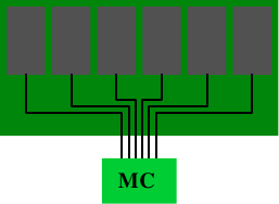
Рис.11.1: Безрегистровый модуль DRAM
С точки зрения электроники, такая схема довольно требовательна. Контроллер памяти должен позволять работать со всеми чипами памяти (их может быть больше тех шести, которые изображены на рисунке). Если в контроллере памяти (MC) есть ограничения, либо если число модулей памяти слишком большое, то такая схема не будет идеальной.
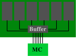
Рис.11.2: Регистровый модуль DRAM
В буферированной (или регистровой) памяти ситуация меняется: в модуле DRAM вместо прямого подключения чипов памяти к контроллеру памяти, чипы подключаются к буферу, который затем, в свою очередь, подключается к контроллеру памяти. В результате значительно снижается сложность электрических соединений. За счет экономии соответствующего числа подключений, возрастает способность контроллера памяти управлять модулями DRAM.
В связи такими преимуществами возникает вопрос: почему не все модули DRAM буферированы? Есть несколько причин. Очевидно, что буферированные модули несколько сложнее, и, следовательно, дороже. Однако, стоимость я- это не единственный фактор. В буфере происходит некоторая задержка сигналов, идущих от чипов памяти; задержка должна быть достаточно большой с тем, чтобы гарантировать, что все сигналы, идущие от чипов памяти, попадут в буфер. В результате в модулях памяти DRAM возрастают задержки. В качестве последнего фактора здесь следует отметить, что из-за использования дополнительной электрической компоненты возрастает энергопотребление. Поскольку буфер должен работать на частоте шины, энергопотребление этого компонента может быть значительным.
Из-за других факторов, связанных с использованием модулей DDR2 и DDR3, как правило, в банке памяти нельзя иметь более двух модулей DRAM. Количество банков (до двух в общераспространенных устройствах) ограничивается количеством контактов контроллера. Большинство контроллеров памяти могут управлять четырьмя модулями DRAM и, следовательно, достаточно использовать безрегисровые модули. В серверных средах с высокими требованиями к памяти ситуация может оказаться другой.
Другой аспект некоторых серверных сред состоит в том, что в них ошибки недопустимы. Ошибки могут возникнуть из-за незначительных изменения поля внутри конденсаторов в ячейках памяти. Люди часто шутят о космической радиации, но это действительно возможно. Вместе с альфа-распадами и другими природными явлениями, они приводят к ошибкам, при которых содержимое ячейки памяти изменяется с 0 на 1 или наоборот. Чем больше используется памяти, тем выше вероятность такого события.
Если такие ошибки неприемлемы, то можно использовать DRAM с технологией ECC (Error Correction Code — код коррекции ошибок). Коды коррекции ошибок позволяют на аппаратном уровне распознать неверное содержимое ячейки памяти и, в некоторых случаях, исправить ошибки. В прошлом ошибки распознавались с помощью проверки четности и, когда обнаруживалась одна ошибка, машину нужно было останавливать. Вместо этого при использовании ECC стало возможным исправлять небольшое количество ошибочных битов. Тем не менее, если количество ошибок слишком большое, доступ к памяти невозможно выполнить правильно, и машина, все же, останавливается. Хотя при использовании модулей DRAM это достаточно маловероятный случай, поскольку в одном модуле должно произойти несколько ошибок.
Когда мы говорим о памяти ECC, мы, на самом деле, не совсем корректны. Проверку ошибок выполняет не память, вместо нее это делает контроллер памяти. Просто в модулях DRAM вместе с реальными данными есть возможность хранить и передавать несколько дополнительных битов, которые не являются данными. Обычно в памяти ECC для каждых 8 битов данных хранится один дополнительный бит. Далее будет разъяснено, почему используются 8 битов.
При записи данных в адрес памяти, контроллер памяти перед тем, как отправлять данные и ECC в шину памяти, на лету вычисляет ECC для нового содержимого. При чтении данных берутся данные и ECC, контроллер памяти вычисляет значение ECC для данных и сравнивает это значение с ECC, полученным из модуля DRAM. Если оба кода ECC совпадут, то это значит, что все хорошо. Если они не совпадают, то контроллер памяти пытается исправить ошибку. Если такое исправление невозможно, то ошибка регистрируется в журнале и, возможно, машина останавливается.
Таблица 11.1: Соотношение ECC и битов данных
| SEC | SEC/DED | |||
|---|---|---|---|---|
| Биты данных W | Биты кода ECC E | Накладные расходы | Биты кода ECC E | Накладные расходы |
| 4 | 3 | 75.0% | 4 | 100.0% |
| 8 | 4 | 50.0% | 5 | 62.5% |
| 16 | 5 | 31.3% | 6 | 37.5% |
| 32 | 6 | 18.8% | 7 | 21.9% |
| 64 | 7 | 10.9% | 8 | 12.5% |
Для корректировки ошибок используются несколько технологий, но для DRAM ECC обычно используются коды Хэмминга. Коды Хэмминга первоначально использовались для кодирования четырех битов данных с возможностью обнаружить и исправить один измененный бит (SEC — коррекция единичной ошибки). Механизм можно легко расширить на большее количество битов данных. Зависимость между количеством битов данных W и количество битов E, используемых для корректировки ошибок, описывается уравнением
E = ⌈log2 (W+E+1)⌉
В результате итеративного решения этого уравнения получаем значения, указанные во второй колонке таблицы 11.1. При наличии дополнительного бита мы можем выявить два измененных бита за счет использования простого бита четности. Тогда эта технология будет называться SEC/DED (Single Error Correction/Double Error Detection — Корректировка одной ошибки/Обнаружение двух ошибок). При наличии этого дополнительного бита мы получаем значения, указанные в четвертом столбце таблицы 11.1. Накладные расходы для W=64 достаточно низкие, а числа (64, кратны 8, так что это естественный выбор для ECC. В большинстве модулей каждый чип памяти составляет 8 битов и, следовательно, любая другая комбинация приведет к менее эффективному решению.
| 7 | 6 | 5 | 4 | 3 | 2 | 1 | |
| Слово ECC | D | D | D | P | D | P | P |
| Четность P1 | D | — | D | — | D | — | P |
| Четность P2 | D | D | — | — | D | P | — |
| Четность P4 | D | D | D | P | — | — | — |
Рис.11.3: Структура матрицы генерации кодов Хемминга
Вычисление кода Хэмминга легко продемонстрировать с помощью кода, использующего W = 4 и E = 3. Мы вычисляем биты четности в стратегических местах в закодированном слове. Принцип показан на рис.11.3. В позициях битов, соответствующих степеням двойки, добавляются биты четности. В сумме четности для первого бита четности P1 учитывается каждый второй бит. В сумме четности для второго бита четности P2 учитываются биты данных 1, 3 и 4 (здесь кодируются как 3, 6 и 7). Подобным образом вычисляется P4.
Вычисление битов четности можно более изящно описать с помощью умножения матриц. Мы создаем матрицу G = [I |A], где I является диагональной матрицей из единиц, а A является матрицей генерации четности, которую можем получить из рис.11.3.
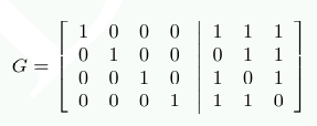
Столбцы матрицы A конструируются из битов, используемых при вычислении P1, P2 и P4. Если мы теперь представим каждый элемент входных данных в виде 4-мерного вектора d, мы можем вычислить r=d⋅G и получить 7-мерный вектор r. Это те данные, которые запоминаются в случае использования ECC DDR.
Чтобы декодировать данные, мы создаем новую матрицу H=[AT|I], где AT является транспонированной матрицей генерации четности, взятой из вычислений G. Т.е. следующее:
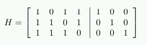
Результат умножения H⋅r показывает, являются ли сохраненные данные дефектными. Если данные не являются дефектными, то произведением будет 3-мерный вектор (0 0 0)T. В противном случае произведение, когда оно интерпретируется как двоичное представление числа, укажет номер столбца с измененным битом.
В качестве примера, предположим, d=(1 0 0 1). Результатом будет
r = (1 0 0 1 0 0 1)
Выполняя проверки с использованием умножения на Н, в результате получаем
Теперь предположим, у нас есть ошибка в хранимых данных и из памяти обратно читаем r’ = (1 0 1 1 0 0 1). В этом случае мы получаем
Вектор не является нулевым вектором и, когда он интерпретируется как число, то s’ имеет значение 5. Это номер бита, который мы изменили в r’ (биты начинаем считать с 1). Контроллер памяти может исправить бит и программы не заметят, что здесь возникла проблема.
Обработка дополнительного бита для части DED лишь немного сложнее. С гораздо большими затратами можно создать коды, с помощью которых можно исправлять два измененных бита и более. Решение о том, необходимо ли это делать, принимается на основе вероятности и рисков. Некоторые производители памяти говорят, что для 256MB памяти ошибка может возникать каждые 750 часов. При удвоении объема памяти, время сокращается на 75%. При достаточном количестве памяти вероятность возникновения ошибки в течение короткого промежутка времени может оказаться существенной и потребуется использовать память ECC RAM. Временной промежуток может оказаться настолько маленьким, что использование SEC/DED становится недостаточным.
Вместо того, чтобы реализовывать еще более сложные схемы исправления ошибок, на серверных материнских платах есть возможность автоматически считывать всю память в течение заданного периода времени. Это означает, что независимо от того, действительно ли память требуется процессору, контроллер памяти читает данные и, если проверка ECC не прошла, записывает исправленные данные обратно в память. До тех пор, пока вероятность будет менее двух ошибок за промежуток времени, необходимый для чтения всего содержимого памяти и записи его обратно, коррекция ошибок с помощью SEC/DED будет вполне разумным решением.
Что касается регистровой DRAM, должен возникнуть вопрос: почему ECC DRAM не является нормой? Ответ на этот вопрос точно такой же, как и на эквивалентный вопрос о регистровой RAM: дополнительный чип памяти повышает стоимость, а вычисление четности увеличивает задержку. Безрегистровая память без ECC может быть гораздо более быстрой. Из-за схожести проблем регистровой DRAM и DRAM с ECC, обычно используют только регистровую DRAM с ECC и безрегистровую DRAM без ECC.
Есть еще один способ преодоления ошибок памяти. Некоторые производители предлагают то, что часто неправильно называется «RAID для памяти», когда данные избыточно распределены по нескольким модулям DRAM, или по крайней мере, чипам памяти. Материнские платы с поддержкой этой функции могут использовать безрегистровые модули DRAM, но увеличение трафика на шинах памяти может свести на нет разницу во времени доступа для модулей DRAM с ECC и без ECC.
Если вам понравилась статья, поделитесь ею с друзьями:
Оглавление
- Вступление
- Коррекция ошибок
- Финансовая сторона
- Тестовый стенд
- Методика тестирования
- Результаты тестирования
- Тест памяти
- 3DMark
- 7Zip
- Cinebench
- CrystalMark
- Fritz
- LinX
- wPrime
- AIDA64 Extreme
- Заключение
Вступление
На сегодняшний день на просторах Рунета можно встретить открытые темы на форумах с вопросами – стоит ли брать рабочую станцию с ECC-памятью или можно обойтись обычной? В данных ветках можно прочесть множество противоречивых утверждений, и часть из них говорит о том, что коррекция ошибок сильно замедляет память, а следовательно и ЦП. Но мало кто это проверял на деле на современных процессорах.
Сегодня мы разберемся в этом вопросе и сравним производительность серверного процессора с обоими типами памяти. Но для начала небольшой экскурс.
Коррекция ошибок
Для чего необходима коррекция? И почему в работе памяти возникают ошибки? Перед ответом на эти вопросы следует разделить ошибки на два типа:
- Аппаратные ошибки;
- Случайные ошибки.
Причиной появления аппаратных ошибок является дефектная микросхема DRAM, а случайные ошибки возникают под воздействием излучения, альфа-частиц, элементарных частиц и прочего. Соответственно, первые в принципе неисправимы – если чип дефектный, то поможет только его замена; а вот вторые могут быть исправлены.
Почему же так необходима коррекция ошибок в рабочих станциях и серверах? Однобитовая ошибка в 64-битном слове меняет содержимое ячейки памяти, а в конечном итоге на жесткий диск может быть записано другое число, другие данные, при этом компьютер не зафиксирует эту подмену. А изменение бита в оперативной памяти может вызвать сбой программы, что для рабочей станции и сервера недопустимо.
рекомендации
-17% на RTX 4070 Ti в Ситилинке
3080 дешевле 70 тр — цены снова пошли вниз
Ищем PHP-программиста для апгрейда конфы
3070 Gainward Phantom дешевле 50 тр
13700K дешевле 40 тр в Регарде
16 видов <b>4070 Ti</b> в Ситилинке — все до 100 тр
3070 Ti дешевле 60 тр в Ситилинке
3070 Gigabyte Gaming за 50 тр с началом
Компьютеры от 10 тр в Ситилинке
3070 дешевле 50 тр в Ситилинке
MSI 3050 за 25 тр в Ситилинке
3060 Gigabyte Gaming за 30 тр с началом
13600K дешевле 30 тр в Регарде
4080 почти за 100тр — дешевле чем по курсу 60
-19% на 13900KF — цены рухнули
12900K за 40тр с началом в Ситилинке
RTX 4090 за 140 тр в Регарде
3060 Ti Gigabyte за 42 тр в Регарде
Для обнаружения изменения битов памяти можно использовать метод подсчета контрольной суммы, но он позволяет лишь обнаруживать ошибки без их исправления.
В свое время было предложено много различных способов решения данной проблемы, но на сегодняшний день наибольшее распространение получил метод коррекции ошибок или ECC (Error-Correcting Code). Данный метод позволяет автоматически исправлять однобитовые ошибки в 64-битном слове – SEC (Single Error Correction) и детектировать двухбитовые – DED (Double Error Detection).
Физическая реализация ECC заключается в размещении дополнительной микросхемы памяти на модуле ОЗУ – соответственно, при одностороннем дизайне модуля памяти вместо восьми чипов располагается девять, а при двустороннем вместо шестнадцати – восемнадцать. Таким образом, ширина модуля становится не 64 бита, а 72 бита.
Метод коррекции ошибок работает следующим образом: при записи 64 бит данных в ячейку памяти происходит подсчет контрольной суммы, составляющей 8 бит. Когда процессор обращается к этим данным и производит считывание, проводится повторный подсчет контрольной суммы и сравнение с исходной. Если суммы не совпадают – произошла ошибка. Если она однобитовая, то неправильный бит исправляется автоматически, если двухбитовая – детектируется и сообщается ОС.
Финансовая сторона
Прежде чем приступить к тестированию, необходимо затронуть финансовый вопрос.
Стоимость обычного модуля памяти DDR3-1600 с напряжением 1.35 В и объемом 8 Гбайт составляет около 3600 рублей, а с коррекцией ошибок – 4800 рублей. На первый взгляд ECC-память выходит на 30-35% дороже, что, в целом, не позволяет их сравнивать в силу существенно большей стоимости последней. Но почему же тогда такой вопрос возникает при сборке рабочей станции? Все просто – необходимо смотреть на данный вопрос шире, а именно – смотреть на общую стоимость рабочей станции.
Ценник однопроцессорной станции на базе четырехъядерного восьмипоточного Xeon (настольные процессоры серий i5 и i7 не поддерживают ECC-память) с 32 Гбайтами памяти, материнской платы с чипсетом C222/С224/С226 (десктопные наборы логики Z87/Z97 и другие также не поддерживают память с коррекцией ошибок) будет превышать 70 000 рублей (при условии, что устанавливаются серверные SSD с повышенным ресурсом). А если включить в эту стоимость и дискретную видеокарту, и прочие сопутствующие компоненты, например, ИБП, то ценник из пятизначного превратится в шестиизначный, перевалив планку в 100 000 рублей.
Покупка 32 Гбайт памяти с коррекцией ошибок потребует дополнительных 4-6 тысяч рублей, что по отношению к общей стоимости рабочей станции не превышает 5%, то есть не является критичным. Также переход от десктопного к серверному железу предоставит и другие преимущества, например: интегрированные графические карты P4600 в процессорах Intel Xeon E3-1200 третьего поколения получили оптимизированные драйверы, которые должны повышать производительность в профессиональных приложениях, например, в CAD; поддержка технологии Intel VT-d, которая позволяет пробрасывать устройства в виртуальную среду, например, видеокарты; прочие серверные технологии – Intel AMT или IPMI, WatchDog и другие, которые также могут оказаться полезными.
Таким образом, хоть и сама ECC-память стоит заметно дороже обычной, в общей стоимости рабочей станции данная статья затрат является несущественной, и переплата не превышает 5%.
Тестовый стенд
Для данного обзора использовалась следующая конфигурация:
- Материнская плата: Supermicro X10SAE (Intel C226, LGA 1150);
- Процессор: Xeon E3-1245V3 (Turbo Boost – off, EIST – off, HT – on);
- Оперативная память:
- 2x Kingston DDR3-1600 ECC 8 Гбайт (KVR16LE11/8 CL11, 1.35 В);
- 2x Kingston DDR3-1600 8 Гбайт (KVR16LN11/8 CL11, 1.35 В);
- ОС: Windows 8.1 Pro 64-bit.
Методика тестирования
В рамках тестирования были произведены замеры производительности как при одноканальном режиме работы ИКП, так и при двухканальном. Суммарный объем ОЗУ составил 8 (один модуль) и 16 Гбайт (два модуля) соответственно.
Программное обеспечение:
- 3DMark 2006 1.2;
- 7Zip 9.20;
- AIDA64 Extreme 5.20.3400;
- Cinebench R15;
- CrystalMark 2004R3;
- Fritz 4.20;
- LinX 0.6.5;
- wPrime 2.10.
Результаты тестирования
Тест памяти
Перед тем, как приступить к тестированию, проведем замер пропускной способности памяти и латентности.

При изучении результатов можно заключить, что производительность ECC- и non-ECC- памяти находится на одном и том же уровне в рамках погрешности.

Если в предыдущем тесте от замера к замеру выигрывал то один, то другой тип памяти, то при замере латентности ECC-память постоянно показывает большие задержки. Но разница несущественна – всего лишь 1 нс.
Таким образом, замер ПС и латентности памяти не показал особых различий между ECC- и non-ECC-памятью. Посмотрим, повторится ли это в последующих тестах.
3DMark
Тестовый пакет 3DMark содержит подтесты как для процессора, так и для графической карты. Здесь и кроется самое интересное – давно известно, что встроенному видеоядру не хватает существующей ПСП в 25.6 Гбайт/с, поэтому именно в графических подтестах можно выявить негативное влияние коррекции ошибок, если оно вообще есть,…

… но разницы нет – что ECC, что non-ECC. Ни процессор, ни интегрированное ядро никак не реагируют на замену обычной памяти на DDR с коррекцией ошибок – результаты одинаковы в рамках погрешности. Среднеарифметическая разница составила 0.02% в пользу ECC-памяти для одноканального режима и 1.6% для двухканального режима.
При этом нельзя сказать, что встроенная видеокарта P4600 не зависит от скорости ОЗУ – при одноканальном доступе общий результат почти на 30% ниже, чем при двухканальном. Другими словами, скорость ОЗУ критична для графического ядра, но сами по себе «ECC-версии» не влияют ни на скорость ОЗУ, ни на видеокарту.
7Zip
Архиваторы, как известно, чувствительны к памяти, поэтому, возможно, здесь получится зафиксировать влияние типа памяти на производительность.

Ситуация с архивацией неоднозначная: с одной стороны – в одноканальном режиме (как при распаковке, так и при сжатии) ECC-память уверенно оказывается медленнее на 2%; с другой – в двухканальном режиме при сжатии ECC-память уверенно быстрее, а при распаковке – медленнее, а среднее арифметическое – быстрее на 0.65%.
Скорее всего, причина в следующем – пропускной способности памяти при одноканальном доступе процессору явно недостаточно, и поэтому чуть большая латентность ECC-памяти сказывается на производительности; а при двухканальном доступе ПСП полностью покрывает нужды CPU и поэтому чуть большая латентность памяти с коррекцией ошибок не сказывается на производительности. В любом случае зафиксировать существенного влияния на скорость архивации не получилось.
Cinebench
Тестовый пакет Cinebench содержит подтест как процессора, так и видеокарты.

Но ни первый, ни вторая никак не отреагировали на ECC-память.
Зато налицо явная зависимость видеокарты от ПСП – при одноканальном доступе результат в OpenGL оказался на 25% ниже, чем при двухканальном. Вспоминая результаты 3DMark и смотря на нынешние, можно заключить, что производительность интегрированной видеокарты хоть и зависит от ПСП, но ECC-память не оказывает на нее негативного влияния.
Error correcting codes (ECCs) are used in computer and communication systems to
improve resiliency to bit flips caused by permanent hardware faults or
transient conditions, such as neutron particles from cosmic rays, known
generally as soft errors. This note
describes the principles of Hamming codes that underpin ECC schemes, ECC codes
are constructed, focusing on single-error correction and double error
detection, and how they are implemented.
ECCs work by adding additional redundant bits to be stored or transported with
data. The bits are encoded as a function of the data in such a way that it is
possible to detect erroneous bit flips and to correct them. The ratio of the
number of data bits to the total number of bits encoded is called the code
rate, with a rate of 1 being a an impossible encoding with no overhead.
Simple ECCs
Parity coding adds a single bit that indicates whether the number of set
bits in the data is odd or even. When the data and parity bit is accessed or
received, the parity can be recomputed and compared. This is sufficient to
detect any odd number of bit flips but not to correct them. For applications
where the error rate is low, so that only single bit flips are likely and
double bit flips are rare enough to be ignored, parity error detection is
sufficient and desirable due to it’s low overhead (just a single bit) and
simple implementation.
Repetition coding simply repeats each data bit a fixed number of times. When
the encoded data is received, if each of the repeated bits are non identical,
an error has occurred. With a repetition of two, single-bit errors can be
detected but not corrected. With a repetition of three, single bit flips can be
corrected by determining each data bit as the majority value in each triple,
but double bit flips are undetectable and will cause an erroneous correction.
Repetition codes are simple to implement but have a high overhead.
Hamming codes
Hamming codes are an efficient family of codes using additional redundant bits to
detect up to two-bit errors and correct single-bit errors (technically, they are
linear error-correcting codes).
In them, check bits are added to data bits to form a codeword, and the
codeword is valid only when the check bits have been generated from the data
bits, according to the Hamming code. The check bits are chosen so that there is
a fixed Hamming distance between any two valid codewords (the number of
positions in which bits differ).
When valid codewords have a Hamming distance of two, any single bit flip will
invalidate the word and allow the error to be detected. For example, the valid
codewords 00 and 11 are separated for single bit flips by the invalid
codewords 01 and 10. If either of the invalid words is obtained an error
has occurred, but neither can be associated with a valid codeword. Two bit
flips are undetectable since they always map to a valid codeword. Note that
parity encoding is an example of a distance-two Hamming code.
00 < Valid codeword
|
10 < Invalid codeword (obtained by exactly 1 bit flip)
|
11 < Valid codeword
With Hamming distance three, any single bit flip in a valid codeword makes an
invalid one, and the invalid codeword is Hamming distance one from exactly one
valid codeword. Using this, the valid codeword can be restored, enabling single
error correction. Any two bit flips map to an invalid codeword, which would
cause correction to the wrong valid codeword.
000 < Valid codeword
 |
001
 |
011
 |
111 < Valid codeword
With Hamming distance four, two bit flips moves any valid codeword Hamming
distance two from exactly two valid codewords, allowing detection of two flips
but not correction. Single bit flips can be corrected as they were for distance
three. Distance-four codes are widely used in computing, where is it often the
case where single errors are frequent, double errors are rare and triple errors
occur so rarely they can be ignored. These codes are referred to as ‘SECDED
ECC’ (single error correction, double error detection).
0000 < Valid codeword
 |
0001
 |
0011 < Two bit flips from either codeword.
 |
0111
 |
1111 < Valid codeword
Double errors can be corrected with a distance-five code, as well as enabling
the detection of triple errors. In general, if a Hamming code can detect $d$
errors, it must have a minimum distance of $d+1$ so there is no way $d$ errors
can change one valid codeword into another one. If a code can correct $d$
errors, it must have a minimum distance of $2d+1$ so that the originating code
is always the closest one. The following table summarises Hamming codes.
| Distance | Max bits corrected | Max bits detected | |
|---|---|---|---|
| 2 | 1 | 0 | Single error detection (eg parity code) |
| 3 | 1 | 1 | Single error correction (eg triple repetition code) |
| 4 | 1 | 2 | Single error correction, double error detection (a ‘SECDED’ code) |
| 5 | 2 | 2 | Double error correction |
| 6 | 2 | 3 | Double error correction, triple error detection |
Creating a Hamming code
A codeword includes the data bits and checkbits. Each check bit corresponds to
a subset of the data bits and it is set when the parity of those data bits is
odd. To obtain a code with a particular Hamming distance, the number of check
bits and their mapping to data bits must be chosen carefully.
To build a single-error correcting (SEC) code that requires Hamming distance
three between valid codewords, it is necessary for:
- The mapping of each data bit to check bits is unique.
- Each data bit to map to at least two check bits.
To see why this works, consider two distinct codewords that necessarily
must have different data bits. If the data bits differ by:
-
1 bit, at least two check bits are flipped, giving a total of three
different bits. -
2 bits, these will cause at least one flip in the check bits since any two
data bits cannot share the same check-bit mapping (ie by taking the XOR of
the two check bit patterns). This also gives a total of three different bits as required. -
3 bits, this is already sufficient to give a Hamming distance of three.
To build a SECDED code that requires Hamming distance of four between valid
codewords, it is necessary for:
- The mapping of each data bit to check bits is unique.
- Each data bit to map to at least three check bits.
- Each check bit pattern to have an odd number of bits set.
Following a similar argument, consider two distinct codewords, data differing by:
-
1 bit flips three check bits, giving a total of four different bits.
-
2 bits flip check bits in two patterns, and since any two odd-length patterns
must have at least two non-overlapping bits, the results is at least two
flipped bits, giving a total of four different bits. For example:
Check bits:  0 1 2 3
data[a]      x x x
data[b]        x x x
-----------  --------
Flips        x     x

Check bits:  0 1 2 3 4
data[a]      x x x
data[b]      x x x x x
----------   ---------
Flips              x x
- 3 bits flip check bits in three patterns, and this time it is possible to
overlap odd-length patterns in such a way that a minimum of 1 bit is flipped.
For example:
Check bits:  0 1 2 3 4
data[a]      x x x
data[b]        x x x
data[c]      x     x x
-----------  ---------
Flips                x

Check bits:  0 1 2 3 4
data[a]      x x x x x
data[b]      x x x
data[c]      x     x x
-----------  ---------
Flips        x
- 4 bits is already sufficient to provide a Hamming distance of four.
An example SEC code for eight data bits with four parity bits:
Check bits:  0 1 2 3
data[0]      x x x
data[1]        x x x
data[2]      x   x x
data[3]      x x   x
data[4]      x x
data[5]        x x
data[6]          x x
data[7]      x     x
An example SECDED code for eight data bits with five parity bits:
Check bits:  0 1 2 3 4
data[0]      x x x
data[1]      x x   x
data[2]      x   x x
data[3]        x x x
data[4]      x x     x
data[5]      x   x   x
data[6]        x x   x
data[7]      x     x x
Note that mappings of data bits to check bits can be chosen flexibly, providing
they maintain the rules that set the Hamming distance. This flexibility is
useful when implementing ECC to reduce the cost of calculating the check bits.
In contrast, many descriptions of ECC that I have found in text books and on
Wikipedia describe a specific
encoding that does not acknowledge this freedom. The encoding they describe
allows the syndrome to be interpreted as the bit index of the single bit error,
by the check bit in position $i$ covering data bits in position $i$.
Additionally, they specify that parity bits are positioned in the codeword at
power-of-two positions, for no apparent benefit.
Implementing ECC
Given data bits and check bits, and mapping of data bits to check bits, ECC
encoding works by calculating the check bits from the data bits, then combining
data bits and check bits to form the codeword. Decoding works by taking the
data bits from a codeword, recalculating the check bits, then calculating the
bitwise XOR between the original check bits and the recalculated ones. This
value is called the syndrome. By inspecting the number of bits set in the
syndrome, it is possible to determine whether there has been an error,
whether it is correctable, and how to correct it.
Using the SEC check-bit encoding above, creating a codeword from data[7:0],
the check bits are calculated as follows (using Verilog syntax):
assign check_word[0] = data[0] ^ data[2] ^ data[3] ^ data[4] ^ data[7];
assign check_word[1] = data[0] ^ data[1] ^ data[3] ^ data[4] ^ data[5];
assign check_word[2] = data[0] ^ data[1] ^ data[2] ^ data[5] ^ data[6];
assign check_word[3] = data[1] ^ data[2] ^ data[3] ^ data[6] ^ data[7];
And the codeword formed by concatenating the check bits and data:
assign codeword = {check[3:0], data[7:0]};
Decoding of a codeword, splits it into the checkword and data bits, recomputes
the check bits and calculates the syndrome:
assign {old_check_word, old_data} = codeword;
assign new_check_word[0] = ...;
assign new_check_word[1] = ...;
assign new_check_word[2] = ...;
assign new_check_word[3] = ...;
assign syndrome = new_check_word ^ old_check_word;
When single bit errors occur, the syndrome will have the bit pattern
corresponding to a particular data bit, so a correction can be applied by
creating a mask to flip the bit in that position:
unique case(syndrome)
  4'b1110: correction = 1<<0;
  4'b0111: correction = 1<<1;
  4'b1011: correction = 1<<2;
  4'b1101: correction = 1<<3;
  4'b1100: correction = 1<<4;
  4'b0110: correction = 1<<5;
  4'b0011: correction = 1<<6;
  4'b1001: correction = 1<<7;
  default: correction = 0;
endcase
And using it to generate the corrected data:
assign corrected_data = data ^ correction;
The value of the syndrome can be further inspected to signal what action has
been taken. If the syndrome is:
- Equal to zero, no error occurred.
- Has one bit set, then this is a flip of a check bit and can be ignored.
- Has a value matching a pattern (three bits set or two bits in the adjacent positions), a correctable error occurred.
- Has a value not matching a pattern (two bits set in the other non-adjacent positions:
4'b1010,4'b0101), or four bits set, a multi-bit uncorrectable error occurred.
The above SECDED check-bit encoding can be implemented in a similar way, but
since it uses only three-bit patterns, mapping syndromes to correction masks
can be done with three-input AND gates:
unique case(syndrome)
  syndrome[0] && syndrome[1] && syndrome[2]: correction = 1<<0;
  syndrome[0] && syndrome[1] && syndrome[3]: correction = 1<<1;
  syndrome[0] && syndrome[2] && syndrome[3]: correction = 1<<2;
  syndrome[1] && syndrome[2] && syndrome[3]: correction = 1<<3;
  syndrome[0] && syndrome[1] && syndrome[4]: correction = 1<<4;
  syndrome[0] && syndrome[2] && syndrome[4]: correction = 1<<5;
  syndrome[1] && syndrome[2] && syndrome[4]: correction = 1<<6;
  syndrome[0] && syndrome[3] && syndrome[4]: correction = 1<<7;
  default:                                   correction = 0;
endcase
And any syndromes with one or two bits set are correctable, and otherwise uncorrectable.
References / further reading
- Error correction code, Wikipedia.
- Hamming code, Wikipedia.
- ECC memory, Wikipedia.
- Error detecting and error correcting codes (PDF),
R. W. Hamming, in The Bell System Technical Journal, vol. 29, no. 2, pp. 147-160, April 1950. - Constructing an Error Correcting Code (PDF),
Andrew E. Phelps, University of Wisconsin, Madison, November 2006.
Please get in touch (mail @ this domain) with any
comments, corrections or suggestions.