Описание одной выборки
Справочный материал.
Описательная статистика
Идея
описательных или дескриптивных статистик
очень проста: вместо того чтобы
рассматривать все
значения переменной (признака), а их
может быть очень много, стоит просмотреть
описательные статистики. Они дают общее
представление о значениях, которые
принимает переменная.
Генеральная
совокупность
это множество всех мыслимых наблюдений,
которые могли бы быть произведены при
данном комплексе условий.
Выборочной
совокупностью
или просто выборкой
называют результаты ограниченного ряда
наблюдений. Выборку рассматривают как
некий эмпирический аналог генеральной
совокупности, с которым чаще всего на
практике имеют дело, поскольку обследование
всей генеральной совокупности бывает
либо слишком трудоемко, либо невозможно.
Объемом
совокупности (выборочной или генеральной)
называют число наблюдений этой
совокупности.
Распределением
признака (переменной) называют
закономерность встречаемости различных
его значений.
Параметры
распределения
(описательные статистики)
это его числовые характеристики,
описывающие распределение. Они указывают,
где “в среднем” располагаются значения
признака, насколько эти значения
изменчивы и наблюдается ли преимущественное
появление определенных значений
признака. В реальных психологических
исследованиях мы оперируем не параметрами,
а их приближенными значениями, так
называемыми оценками
параметров. Это объясняется ограниченностью
обследованных выборок. Чем больше
выборка, тем ближе могут быть оценки
параметра к его истинному значению. В
дальнейшем, говоря о параметрах, мы
будем иметь в виду их оценки. Параметры
определяют то, что называется средней
тенденцией, разброс значений и форму
распределения.
В
программе STATISTICA
(модуль Basic
Statistics
Descriptive
Statistics)
можно посчитать следующие описательные
статистики:
-
Количество
значений переменной (Valid
N) -
Сумма
всех значений переменной (Sum) -
Минимум
и максимум (Minimum
& Maximum)
— это минимальное и максимальное
значения переменной. -
Среднее
(Mean)
— сумма значений переменной, деленная
на N
(число значений переменной). Обычно
обозначается
 .
. -
Дисперсия
(Variance)
и стандартное отклонение (Standard
deviation)
— наиболее
часто используемые меры изменчивости
переменной. Дисперсия меняется от нуля
до бесконечности. Крайнее значение 0
означает отсутствие изменчивости,
когда значения переменной постоянны.

Стандартное
отклонение вычисляется как корень
квадратный из дисперсии. Чем выше
дисперсия или стандартное отклонение,
тем сильнее разбросаны значения
переменной относительно среднего. Часто
стандартное отклонение — более удобная
характеристика, т. к измерена в тех же
единицах, что исходная величина.
-
Медиана
(Median)
разбивает выборку на две равные части.
Половина значений переменной лежит
ниже медианы, половина — выше. Медиана
дает общее представление о том, где
сосредоточены значения переменной,
иными словами, где находится ее центр.
В некоторых случаях, например, при
описании доходов населения, медиана
более удобна, чем среднее. -
Мода
(Mode)
представляет собой максимально часто
встречающееся значение переменной.
Если распределение имеет несколько
мод, то говорят, что оно мультимодально
или многомодально (имеет два или более
«пика»). Мультимодальность распределения
дает важную информацию о природе
исследуемой переменной. Например, в
социологических опросах, если переменная
представляет собой предпочтение или
отношение к чему-либо, то мультимодальность
может означать, что существует несколько
определенно различных мнений.
Мультимодальность также служит
индикатором того, что выборка не является
однородной и наблюдения, возможно,
порождены двумя или более «наложенными»
распределениями.
-
Доверительный
интервал (95%
confidence
limits
of
mean)
для среднего представляет интервал
значений вокруг оценки, где с данным
уровнем доверия находится «истинное»
(неизвестное) среднее генеральной
совокупности. Например, если среднее
выборки равно 23, а нижняя и верхняя
границы доверительного интервала с
уровнем p=.95
равны 19 и 27 соответственно, то можно
заключить, что с вероятностью 95% интервал
с границами 19 и 27 накрывает среднее
генеральной совокупности. Если вы
установите больший уровень доверия,
то интервал станет шире, поэтому
возрастает вероятность, с которой он
«накрывает» неизвестное среднее
генеральной совокупности, и наоборот.
Ширина доверительного интервала зависит
от объема или размера выборки, а также
от разброса (изменчивости) данных.
Увеличение размера выборки делает
оценку среднего более надежной.
Увеличение разброса наблюдаемых
значений уменьшает надежность оценки.
Вычисление доверительных интервалов
основывается на предположении
нормальности наблюдаемых величин. Если
это предположение не выполнено, то
оценка может оказаться плохой, особенно
для малых выборок. При увеличении объема
выборки, скажем, до 100 или более, качество
оценки улучшается и без предположения
нормальности выборки.
-
Стандартная
ошибка среднего значения (Standard
error
of
mean)
– это стандартное отклонение, деленное
на квадратный корень из объема выборки.
В интервале шириной, равной удвоенной
стандартной ошибке, отложенному вокруг
среднего значения, располагается
среднее значение генеральной совокупности
с вероятностью примерно 67%. Стандартная
ошибка, как и стандартное отклонение,
может использоваться в качестве меры
разброса переменной. По так называемому
правилу кулака, в одном диапазоне
стандартного отклонения (охватывающем
ширину стандартного отклонения в обе
стороны от среднего значения) располагается
примерно 67% значений, в диапазоне
удвоенного стандартного отклонения –
примерно 95%, а в диапазоне утроенного
стандартного отклонения – примерно
99% значений. С другой стороны, стандартная
ошибка позволяет задать доверительный
интервал для среднего значения. В
диапазоне удвоенной стандартной ошибки
по обе стороны от среднего значения с
вероятностью примерно 95% находится
среднее значение генеральной совокупности.
С вероятностью примерно 99% оно лежит в
диапазоне утроенной стандартной ошибки.
Обычно указывают только одну из мер
изменчивости.
-
Квартили
представляют собой значения, которые
делят две половины выборки (разбитые
медианой) еще раз пополам. Таким образом,
медиана и квартили делят диапазон
значений переменной на четыре равные
части. Различают верхний квартиль,
который больше медианы и делит пополам
верхнюю
часть выборки (значения переменной
больше медианы), и нижний квартиль,
который меньше медианы и делит пополам
нижнюю часть
выборки
(Lower
and Upper quartiles).
Нижний
квартиль часто обозначают символом
25%, это означает, что 25%
значений
переменной меньше нижнего квартиля.
Верхний квартиль часто обозначают
символом 75%, это означает, что 75% значений
переменной меньше верхнего квартиля.
-
Размах
(Range)
разница между наибольшим и наименьшим
значением переменной
-
Квартильный
(внутриквартильный) размах
(Quartile
Range)
равен разности значений верхнего и
нижнего квартиля. Таким образом, это
интервал, содержащий медиану, в который
попадает 50% наблюдений.
-
Асимметрия
(Skewness),
или коэффициент асимметрии, является
мерой несимметричности распределения.
Если этот коэффициент значительно
отличается от 0, распределение является
асимметричным, т.е. несимметричным.
Асимметрия вычисляется по формуле:
А
= ,
,
где
![]() – среднее,
– среднее,
стандартное отклонение, N
число наблюдений.
-
Эксцесс
(Kurtosis),
или коэффициент эксцесса измеряет
остроту пика распределения. Оценка
эксцесса вычисляется по формуле:
E=
Коэффициент
эксцесса равен нулю, если наблюдения
подчиняются нормальному распределению.
Если он значительно отличается от нулю,
гипотезу о том, что данные взяты из
нормального распределенной генеральной
совокупности, следует отвергнуть.
-
Стандартные
ошибки асимметрии и эксцесса (Standard
error
of
skewness,
Standard
error
of
kurtosis)
– это и есть стандартные ошибки
асимметрии и эксцесса, аналогичные
стандартной ошибке среднего.
Лабораторная
работа 2.
описательная
статистика и графики
Задание
2: данные о стаже и зарплате
1.
Загрузите файл данных.
-
Скопируйте
Empl_Data.sta
в свою рабочую папку. -
В
STATISTICA
Module Switcher
выберите
модуль
Basic
Statistics
и
пока
нажмите
кнопку
Cancel. -
Загрузите
файл
Empl_Data.sta: File
Open
Data …
В файле
приведены следующие данные
ID
– номер
испытуемого;
Gender
– пол
испытуемого;
Educ
– образование
испытуемого (количество лет, которые
человек потратил на учебу);
JCAT
– вид профессиональной деятельности
(1 – секретари, 2– охранники, 3 – менеджеры);
Salary
– зарплата
в настоящий момент (тыс. долларов в год);
SAL_BEG–
начальная зарплата на этой работе (тыс.
долларов в год);
JTIME
– трудовой стаж на данном рабочем месте
(число месяцев);
PREVEX
– предыдущий опыт – стаж до поступления
на данную работу (число месяцев);
MINORITY
– принадлежит ли испытуемый к национальному
меньшинству (0 – нет, 1 – да).
2. Посчитайте всю
описательную статистику, которую можно
считать, для всех переменных.
2.1.
Сначала выберем переменные Analysis
Descriptive
Statistics
Variables
(кнопка слева вверху)
….
2.2.
В разделе Statistics
нажимаем кнопку More
statistics
и выбираем те параметры, которые нам
нужны. Если надо посчитать все, можно
нажать на кнопку All.
Затем нажимаем кнопку ОК
и опять попадаем в окно Descriptive
Statistics.
В том же разделе Statistics
можно выбрать доверительный интервал
(Conf.
limits
for
means,
Interval),
если не устраивает 95%, заданный по
умолчанию.
2.3.
Чтобы посчитать описательную статистику
можно нажать кнопку ОК
или кнопку Detailed
Descriptive
Statistics.
Получится таблица для всех переменных
со всеми статистиками.
6.2. Вывод статистических характеристик
Чтобы получить описательную статистику числовых переменных, можно щелкнуть в диалоге Frequencies на кнопке Statistics… (Статистика).
Откроется диалоговое окно Frequencies: Statistics (Частоты: Статистика).

Рис. 6.2: Диалоговое окно frequencies: Statistics
В группе Percentile Values (Значения процентилей) можно выбрать следующие варианты:
-
Quartiles (Квартили): Будут показаны первый, второй и третий квартили.
Первый квартиль (Q1) — это точка на шкале измеренных значений, ниже (левее) которой располагаются 25% измеренных значений.
Второй квартиль (Q2) — это точка, ниже которой располагаются 50% измеренных значений. Второй квартиль также называется медианой.
Третий квартиль (Q3) — это точка на шкале измеренных значений, ниже которой располагаются 75% значений.
Если данные имеются только в форме порядкового отношения, то качестве меры разброса используется межквартильная широта. Она определяется как

-
Cut points (Точки раздела): Будут вычислены значения процентилей, разделяющие выборку на группы наблюдений, которые имеют одинаковую ширину, то есть включают одно
и то же количество измеренных значений. По умолчанию предлагается количество групп 10. Если задать, к примеру, 4, то будут показаны квартили, то есть квартили соответствуют процентилям 25, 50 и 75.
Видно, что число показываемых процентилей на единицу меньше заданного числа групп. -
Percentile(s) (Процентили): Здесь имеются в виду значения процентилей, определяемые пользователем. Введите значение процентиля в пределах от 0 до 100 и щелкните на кнопке Add (Добавить).
Повторите эти действия для всех желаемых значений процентилей. Значения в порядке возрастания будут показаны в списке. Например, если ввести значения 25, 50 и 75, то мы получим квартили.
Можно задавать любые значения процентилей, например, 37 и 83. В первом случае (37) будет показано значение выбранной переменной, ниже которого лежат 37% значений, а во втором случае (83) —
значение, ниже которого располагаются 83% значений.
В группе Dispersion (Разброс) можно выбрать следующие меры разброса:
-
Std. deviation (Стандартное отклонение) — это мера разброса измеренных величин; оно равно квадратному корню из дисперсии. В интервале шириной, равной удвоенному стандартному отклонению,
который отложен по обе стороны от среднего значения, располагается примерно 67% всех значений выборки, подчиняющейся нормальному распределению. -
Variance (Дисперсия) — это квадрат стандартного отклонения и, следовательно, эта характеристика также является мерой разброса измеренных величин. О
на определяется как сумма квадратов отклонений всех измеренных значений от их среднеарифметического значения, деленная на количество измерений минус 1. -
Range (Размах) — это разница между наибольшим значением (максимумом) и наименьшим значением (минимумом).
-
Minimum (Минимум) — Наименьшее значение.
-
Maximum (Максимум) — Наибольшее значение.
-
S.E. mean (Стандартная ошибка среднего значения) — В интервале шириной, равной удвоенной стандартной ошибке, отложенному вокруг среднего значения,
располагается среднее значение генеральной совокупности с вероятностью примерно 67%. Стандартная ошибка определяется как стандартное отклонение, деленное на квадратный корень из объема выборки.
Обычно мерами разброса переменных, относящихся к интервальной шкале и подчиняющихся нормальному распределению, служат стандартное отклонение и стандартная ошибка.
Как было сказано выше, стандартное отклонение позволяет задать диапазон разброса отдельных значений. По так называемому правилу кулака, в одном диапазоне стандартного отклонения
(охватывающем ширину стандартного отклонения в обе стороны от среднего значения) располагается примерно 67% значений, в диапазоне удвоенного стандартного отклонения — примерно 95%,
а в диапазоне утроенного стандартного отклонения — примерно 99% значений.
С другой стороны, стандартная ошибка позволяет задать доверительный интервал для среднего значения. В диапазоне удвоенной стандартной ошибки по обе стороны от среднего значения
с вероятностью примерно 95% находится среднее значение генеральной совокупности. С вероятностью примерно 99% она лежит в диапазоне утроенной стандартной ошибки.
Часто указывают только одну из этих двух мер разброса, обычно — стандартную ошибку, так как ее значение меньше. Во всех случаях следует точно выяснить, какая из мер разброса имеется в виду.
В группе Central Tendency (Средние) можно выбрать следующие характеристики:
-
Mean (Среднее значение) — это арифметическое среднее измеренных значений; оно определяется как сумма значений, деленная на их количество.
Например, если имеется 12 измеренных значений и их сумма составляет 600, то среднее значение будет х = 600 : 12 = 50. -
Median (Медиана) — это точка на шкале измеренных значений, выше и ниже которой лежит по половине всех измеренных значений. Например, если измеренные значения таковы:
37854639284,
то сначала они располагаются в порядке возрастания: 23344567889.
В данном случае медианой будет значение 5. Всего у нас 11 измеренных значений, следовательно, медианой является шестое значение. Выше него располагается 5 значений, и ниже — тоже 5.
При нечетном количестве значений медиана всегда будет совпадать с одним из измеренных значений. При четном количестве медиана будет средним арифметическим двух соседних значений.
Например, если имеются следующие измеренные значения:
3445678899
то медиана в этом случае будет равна: (6 + 7) : 2 = 6,5.
-
Mode (Мода) — это значение, которое наиболее часто встречается в выборке. Если одна и та же наибольшая частота встречается у нескольких значений, то выбирается наименьшее из них.
-
Sum (Сумма) — сумма всех значений.
В группе Distribution (Распределение) можно выбрать следующие меры несимметричности распределения:
-
Skewness (Коэффициент асимметрии) — это мера отклонения распределения частоты от симметричного распределения, то есть такого, у которого на одинаковом удалении от среднего значения
по обе стороны выборки данных располагается одинаковое количество значений. Если наблюдения подчиняются нормальному распределению, то асимметрия равна нулю.
Для проверки на нормальное распределение можно применять следующее правило: Если асимметрия значительно отличается от нуля, то гипотезу о том, что данные взяты из нормально распределенной
генеральной совокупности, следует отвергнуть. Если вершина асимметричного распределения сдвинута к меньшим значениям, то говорят о положительной асимметрии, в противоположном случае — об отрицательной. -
Kurtosis (Коэффициент вариации или эксцесс) — указывает, является ли распределение пологим (при большом значении коэффициента) или крутым. Коэффициент вариации равен нулю,
если наблюдения подчиняются нормальному распределению. Поэтому для проверки на нормальное распределение можно применять еще одно правило: Если коэффициент вариации значительно отличается от нуля,
то гипотезу о том, что данные взяты из нормально распределенной генеральной совокупности, следует отвергнуть.
Как правило, для переменных, относящихся к интервальной шкале и подчиняющихся нормальному распределению, в качестве основной характеристики используют среднее значение,
а в качестве меры разброса — стандартное отклонение или стандартную ошибку. Для порядковых или интервальных переменных, не подчиняющихся нормальному распределению —
соответственно медиану или первый и третий квартили. Для переменных относящихся к номинальной шкале, нельзя дать других значимых характеристик кроме моды.
В диалоге есть еще один флажок:
-
Values are group midpoints (Значения являются средними точками групп): Если установить этот флажок, то при вычислении медианы и остальных значений процентилей оценки
этих характеристик будут определяться для концентрированных данных. Этому вопросу посвящен отдельный раздел.
Для переменной alter (возраст) мы определим следующие характеристики: среднее значение, медиану, моду, квартили, стандартное отклонение, дисперсию, размах, минимум, максимум,
стандартную ошибку, асимметрию и эксцесс. Поступите следующим образом:
-
Выберите в меню команды Analyze (Анализ) / Descriptive Statistics (Дескриптивные статистики) / Frequencies… (Частоты)
-
В диалоге Frequencies щелкните на кнопке Reset (Сброс), чтобы отменить прежние настройки.
-
Перенесите переменную alter в список выходных переменных.
-
Щелкните на кнопке Statistics… (Статистика).
-
В диалоге Frequencies: Statistics установите флажки желаемых характеристик. Затем щелкните на кнопке Continue (Продолжить). Вы вернетесь в диалог Frequencies.
-
В диалоге Frequencies деактивируйте опцию Display frequency tables (Показывать частотные таблицы). Щелкните на кнопке ОК.
В окне просмотра появятся следующие результаты:
Statistics (Статистика)
Alter
| N | Valid (Допустимые) | 106 |
| Missing (Утерянные) | 2 | |
| Mean (Среднее значение) | 22,24 | |
| Std. Error of Mean (Стандартная ошибка среднего) | 21 | |
| Median (Медиана) | 22,00 | |
| Mode (Мода) | 21 | |
| Std. Deviation (Стандартное отклонение) | 2,189 | |
| Variance (Дисперсия) | 4,791 | |
| Skewness (Асимметрия) | 0,859 | |
| Std. Error of Skewness (Стандартная ошибка асимметрии) | 0,235 | |
| Kurtosis (Коэффициент вариации / Эксцесс) | 1,042 | |
| Std. Error of Kurtosis (Стандартная ошибка эксцесса) | 0,465 | |
| Range (Размах) | 11 | |
| Minimum (Минимум) | 18 | |
| Maximum (Максимум) | 29 | |
| Percentiles (Процентили) | 25 | 21,00 |
| 50 | 22,00 | |
| 75 | 23,00 |
Респонденты опроса о психическом состоянии и социальном положении имеют средний возраст 22,24 года. Медиана составляет 22. Большинству респондентов 21 год (это мода).
Самому молодому респонденту 18 лет (минимум), самому старшему — 29 лет (максимум). Самый старший респондент на 11 лет старше самого молодого (размах).
Стандартное отклонение составляет 2,19. Следовательно, дисперсия — квадрат стандартного отклонения — равна (2,19)2 = 4,79.
Асимметрия и коэффициент вариации даны со соответсвующими стандартными ошибками.
Skewness quantifies the asymmetry of a distribution of a set of values. GraphPad Prism can compute the skewness as part of the Column Statistics analysis.
How skewness is computed
Understanding how skewness is computed can help you understand what it means. These steps compute the skewness of a distribution of values:
- We want to know about symmetry around the sample mean. So the first step is to subtract the sample mean from each value, The result will be positive for values greater than the mean, negative for values that are smaller than the mean, and zero for values that exactly equal the mean.
- To compute a unitless measures of skewness, divide each of the differences computed in step 1 by the standard deviation of the values. These ratios (the difference between each value and the mean divided by the standard deviation) are called z ratios. By definition, the average of these values is zero and their standard deviation is 1.
- For each value, compute z3. Note that cubing values preserves the sign. The cube of a positive value is still positive, and the cube of a negative value is still negative.
- Average the list of z3 by dividing the sum of those values by n-1, where n is the number of values in the sample. If the distribution is symmetrical, the positive and negative values will balance each other, and the average will be close to zero. If the distribution is not symmetrical, the average will be positive if the distribution is skewed to the right, and negative if skewed to the left. Why n-1 rather than n? For the same reason that n-1 is used when computing the standard deviation.
- Correct for bias. For reasons that I do not really understand, that average computed in step 4 is biased with small samples — its absolute value is smaller than it should be. Correct for the bias by multiplying the mean of z3 by the ratio n/(n-2). This correction increases the value if the skewness is positive, and makes the value more negative if the skewness is negative. With large samples, this correction is trivial. But with small samples, the correction is substantial.
Interpreting skewness
The basics:
- A symmetrical distribution has a skewness of zero.
- An asymmetrical distribution with a long tail to the right (higher values) has a positive skew.
- An asymmetrical distribution with a long tail to the left (lower values) has a negative skew.
- The skewness is unitless.
- Any threshold or rule of thumb is arbitrary, but here is one: If the skewness is greater than 1.0 (or less than -1.0), the skewness is substantial and the distribution is far from symmetrical.
How useful is it to assess skewness? Not very, I think. The numerical value of the skewness does not really answer any of these questions:
- Does the distribution deviate enough from a Gaussian distribution that parametric tests will give invalid results?
- Would the distribution be closer to Gaussian if the data were transformed by taking the logarithm (or reciprocal, or another transform) of all the values?
- Is the skewness due to one or a few outliers?
The skewness doesn’t directly answer any of those questions. Note that the D’ Agostino and Pearson omnibus normality test (a choice within Prism’s column statistics analysis) is a normality test that combines the skewness with the kurtosis (a measure of how far the shape of the distribution deviates from the bell shape of a Gaussian distribution), and so tries to answer the first question.
The definition of the skewness is part of a mathematical progression. The standard deviation is computed by first summing the squares of he differences each value and the mean. The skewness is computed by first summing the cube of those distances. And the kurtosis is computed by first summing the fourth power of those distances.
While there are good reasons for computing the standard deviation by squaring the deviations, there doesn’t appear to be a deeper meaning to summing the cube of the differences between each value and the mean. Since the skewness is computed based on cubes, a value that is twice as far from the mean as another value increases the skewness eight times as much as that other value (because 23=8). I don’t see why alternative definitions of skewness where that factor is some other value (4, or 7 or 10 or any other value greater than 1) wouldn’t be just as informative and useful.
Multiple definitions of skewness
Skewness has been defined in multiple ways. The method used by Prism (and described above) is the most common method. It is identical to the skew() function in Excel. This value of skewness is often abbreviated g1.
The confidence interval of skewness
Whenever a value is computed from a sample, it helps to compute a confidence interval. In most cases, the confidence interval is computed from a standard error. The standard error of skewness (SES) depends on sample size. Prism does not calculate it, but it can be computed easily by hand using this formula:
.gif)
The margin of error equals 1.96 times that value, and the confidence interval for the skewness equals the computed skewness plus or minus the margin of error. This table gives the standard error and margin of error for various sample sizes.
| n | SE of skewness | Margin of error |
| 3 | 1.225 | 2.400 |
| 4 | 1.014 | 1.988 |
| 5 | 0.913 | 1.789 |
| 6 | 0.845 | 1.657 |
| 7 | 0.794 | 1.556 |
| 8 | 0.752 | 1.474 |
| 9 | 0.717 | 1.406 |
| 10 | 0.687 | 1.347 |
| 15 | 0.580 | 1.137 |
| 20 | 0.512 | 1.004 |
| 25 | 0.464 | 0.909 |
| 50 | 0.337 | 0.660 |
| 100 | 0.241 | 0.473 |
| 200 | 0.172 | 0.337 |
| 300 | 0.141 | 0.276 |
| 400 | 0.122 | 0.239 |
| 500 | 0.109 | 0.214 |
| 1000 | 0.077 | 0.152 |
| 2500 | 0.049 | 0.096 |
| 5000 | 0.035 | 0.068 |
| 10000 | 0.024 | 0.048 |
The standard errors are valid for normal distributions, but not for other distributions. To see why, you can run the following code (which uses the spssSkewKurtosis function shown above) to estimate the true confidence level of the interval obtained by taking the kurtosis estimate plus or minus 1.96 standard errors:
set.seed(12345)
Nsim = 10000
Correct = numeric(Nsim)
b1.ols = numeric(Nsim)
b1.alt = numeric(Nsim)
for (i in 1:Nsim) {
 Data = rnorm(1000)
 Kurt = spssSkewKurtosis(Data)[2,1]
 seKurt =  spssSkewKurtosis(Data)[2,2]
  LowerLimit = Kurt -1.96*seKurt
  UpperLimit = Kurt +1.96*seKurt
  Correct[i] = LowerLimit <= 0 & 0 <= UpperLimit
 }

TrueConfLevel = mean(Correct)
TrueConfLevel
This gives you 0.9496, acceptably close to the expected 95%, so the standard errors work as expected when the data come from a normal distribution. But if you change Data = rnorm(1000) to Data = runif(1000), then you are assuming that the data come from a uniform distribution, whose theoretical (excess) kurtosis is -1.2. Making the corresponding change from Correct[i] = LowerLimit <= 0 & 0 <= UpperLimit to Correct[i] = LowerLimit <= -1.2 & -1.2 <= UpperLimit gives the result 1.0, meaning that the 95% intervals were always correct, rather than correct for 95% of the samples. Hence, the standard error seems to be overestimated (too large) for the (light-tailed) uniform distribution.
If you change Data = rnorm(1000) to Data = rexp(1000), then you are assuming that the data come from an exponential distribution, whose theoretical (excess) kurtosis is 6.0. Making the corresponding change from Correct[i] = LowerLimit <= 0 & 0 <= UpperLimit to Correct[i] = LowerLimit <= 6.0 & 6.0 <= UpperLimit gives the result 0.1007, meaning that the 95% intervals were correct only for 10.07% of the samples, rather than correct for 95% of the samples. Hence, the standard error seems to be underestimated (too small) for the (heavy-tailed) exponential distribution.
Those standard errors are grossly incorrect for non-normal distributions, as the simulation above shows. Thus, the only use of those standard errors is to compare the estimated kurtosis with the expected theoretical normal value (0.0); e.g., using a test of hypothesis. They cannot be used to construct a confidence interval for the true kurtosis.
For the planarity measure in graph theory, see Graph skewness.

Example distribution with positive skewness. These data are from experiments on wheat grass growth.
In probability theory and statistics, skewness is a measure of the asymmetry of the probability distribution of a real-valued random variable about its mean. The skewness value can be positive, zero, negative, or undefined.
For a unimodal distribution, negative skew commonly indicates that the tail is on the left side of the distribution, and positive skew indicates that the tail is on the right. In cases where one tail is long but the other tail is fat, skewness does not obey a simple rule. For example, a zero value means that the tails on both sides of the mean balance out overall; this is the case for a symmetric distribution, but can also be true for an asymmetric distribution where one tail is long and thin, and the other is short but fat.
Introduction[edit]
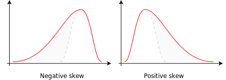
Consider the two distributions in the figure just below. Within each graph, the values on the right side of the distribution taper differently from the values on the left side. These tapering sides are called tails, and they provide a visual means to determine which of the two kinds of skewness a distribution has:
- negative skew: The left tail is longer; the mass of the distribution is concentrated on the right of the figure. The distribution is said to be left-skewed, left-tailed, or skewed to the left, despite the fact that the curve itself appears to be skewed or leaning to the right; left instead refers to the left tail being drawn out and, often, the mean being skewed to the left of a typical center of the data. A left-skewed distribution usually appears as a right-leaning curve.[1]
- positive skew: The right tail is longer; the mass of the distribution is concentrated on the left of the figure. The distribution is said to be right-skewed, right-tailed, or skewed to the right, despite the fact that the curve itself appears to be skewed or leaning to the left; right instead refers to the right tail being drawn out and, often, the mean being skewed to the right of a typical center of the data. A right-skewed distribution usually appears as a left-leaning curve.[1]
Skewness in a data series may sometimes be observed not only graphically but by simple inspection of the values. For instance, consider the numeric sequence (49, 50, 51), whose values are evenly distributed around a central value of 50. We can transform this sequence into a negatively skewed distribution by adding a value far below the mean, which is probably a negative outlier, e.g. (40, 49, 50, 51). Therefore, the mean of the sequence becomes 47.5, and the median is 49.5. Based on the formula of nonparametric skew, defined as  the skew is negative. Similarly, we can make the sequence positively skewed by adding a value far above the mean, which is probably a positive outlier, e.g. (49, 50, 51, 60), where the mean is 52.5, and the median is 50.5.
As mentioned earlier, a unimodal distribution with zero value of skewness does not imply that this distribution is symmetric necessarily. However, a symmetric unimodal or multimodal distribution always has zero skewness.
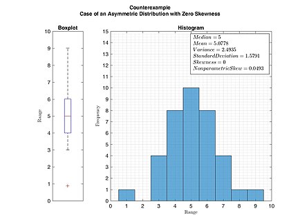
Example of an asymmetric distribution with zero skewness. This figure serves as a counterexample that zero skewness does not imply symmetric distribution necessarily. (Skewness was calculated by Pearson’s moment coefficient of skewness.)
Relationship of mean and median[edit]
The skewness is not directly related to the relationship between the mean and median: a distribution with negative skew can have its mean greater than or less than the median, and likewise for positive skew.[2]

A general relationship of mean and median under differently skewed unimodal distribution
In the older notion of nonparametric skew, defined as where  is the mean,
  is the median, and
  is the standard deviation, the skewness is defined in terms of this relationship: positive/right nonparametric skew means the mean is greater than (to the right of) the median, while negative/left nonparametric skew means the mean is less than (to the left of) the median. However, the modern definition of skewness and the traditional nonparametric definition do not always have the same sign: while they agree for some families of distributions, they differ in some of the cases, and conflating them is misleading.
If the distribution is symmetric, then the mean is equal to the median, and the distribution has zero skewness.[3] If the distribution is both symmetric and unimodal, then the mean = median = mode. This is the case of a coin toss or the series 1,2,3,4,… Note, however, that the converse is not true in general, i.e. zero skewness (defined below) does not imply that the mean is equal to the median.
A 2005 journal article points out:[2]
Many textbooks teach a rule of thumb stating that the mean is right of the median under right skew, and left of the median under left skew. This rule fails with surprising frequency. It can fail in multimodal distributions, or in distributions where one tail is long but the other is heavy. Most commonly, though, the rule fails in discrete distributions where the areas to the left and right of the median are not equal. Such distributions not only contradict the textbook relationship between mean, median, and skew, they also contradict the textbook interpretation of the median.

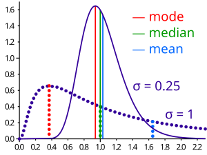
Distribution of adult residents across US households
For example, in the distribution of adult residents across US households, the skew is to the right. However, since the majority of cases is less than or equal to the mode, which is also the median, the mean sits in the heavier left tail. As a result, the rule of thumb that the mean is right of the median under right skew failed.[2]
Definition[edit]
Fisher’s moment coefficient of skewness[edit]
The skewness of a random variable X is the third standardized moment  , defined as:[4][5]
![{displaystyle {tilde {mu }}_{3}=operatorname {E} left[left({frac {X-mu }{sigma }}right)^{3}right]={frac {mu _{3}}{sigma ^{3}}}={frac {operatorname {E} left[(X-mu )^{3}right]}{(operatorname {E} left[(X-mu )^{2}right])^{3/2}}}={frac {kappa _{3}}{kappa _{2}^{3/2}}}}](https://wikimedia.org/api/rest_v1/media/math/render/svg/30324ac725e96b88638a0fc86f201b174082cbc7)
where μ is the mean, σ is the standard deviation, E is the expectation operator, μ3 is the third central moment, and κt are the t-th cumulants. It is sometimes referred to as Pearson’s moment coefficient of skewness,[5] or simply the moment coefficient of skewness,[4] but should not be confused with Pearson’s other skewness statistics (see below). The last equality expresses skewness in terms of the ratio of the third cumulant κ3 to the 1.5th power of the second cumulant κ2. This is analogous to the definition of kurtosis as the fourth cumulant normalized by the square of the second cumulant.
The skewness is also sometimes denoted Skew[X].
If σ is finite, μ is finite too and skewness can be expressed in terms of the non-central moment E[X3] by expanding the previous formula,
![{displaystyle {begin{aligned}{tilde {mu }}_{3}&=operatorname {E} left[left({frac {X-mu }{sigma }}right)^{3}right]\&={frac {operatorname {E} [X^{3}]-3mu operatorname {E} [X^{2}]+3mu ^{2}operatorname {E} [X]-mu ^{3}}{sigma ^{3}}}\&={frac {operatorname {E} [X^{3}]-3mu (operatorname {E} [X^{2}]-mu operatorname {E} [X])-mu ^{3}}{sigma ^{3}}}\&={frac {operatorname {E} [X^{3}]-3mu sigma ^{2}-mu ^{3}}{sigma ^{3}}}.end{aligned}}}](https://wikimedia.org/api/rest_v1/media/math/render/svg/77a8f1e4f233c410e85698ca11d163f6f81c5e5f)
Examples[edit]
Skewness can be infinite, as when
![Pr left[ X > x right]=x^{-2}mbox{ for }x>1, Pr[X<1]=0](https://wikimedia.org/api/rest_v1/media/math/render/svg/5b85499e724ce781c6321eaeeaff9f20ecee2b83)
where the third cumulants are infinite, or as when
![Pr[X<x]=(1-x)^{-3}/2{mbox{ for negative }}x{mbox{ and }}Pr[X>x]=(1+x)^{-3}/2{mbox{ for positive }}x.](https://wikimedia.org/api/rest_v1/media/math/render/svg/4c82a811b61702e6fdfff80fa0aa14a86a6e2f16)
where the third cumulant is undefined.
Examples of distributions with finite skewness include the following.
- A normal distribution and any other symmetric distribution with finite third moment has a skewness of 0
- A half-normal distribution has a skewness just below 1
- An exponential distribution has a skewness of 2
- A lognormal distribution can have a skewness of any positive value, depending on its parameters
Sample skewness[edit]
For a sample of n values, two natural estimators of the population skewness are[6]
![{displaystyle b_{1}={frac {m_{3}}{s^{3}}}={frac {{tfrac {1}{n}}sum _{i=1}^{n}(x_{i}-{overline {x}})^{3}}{left[{tfrac {1}{n-1}}sum _{i=1}^{n}(x_{i}-{overline {x}})^{2}right]^{3/2}}}}](https://wikimedia.org/api/rest_v1/media/math/render/svg/622780d6e0eb8322149ef5e232e5c8a6ce523e33)
and
![{displaystyle g_{1}={frac {m_{3}}{m_{2}^{3/2}}}={frac {{tfrac {1}{n}}sum _{i=1}^{n}(x_{i}-{overline {x}})^{3}}{left[{tfrac {1}{n}}sum _{i=1}^{n}(x_{i}-{overline {x}})^{2}right]^{3/2}}},}](https://wikimedia.org/api/rest_v1/media/math/render/svg/b632e0d32061f78e178eb9a1c6e22da4324e817c)
where  is the sample mean, s is the sample standard deviation, m2 is the (biased) sample second central moment, and m3 is the sample third central moment.[6]
  is a method of moments estimator.
Another common definition of the sample skewness is[6][7]

where  is the unique symmetric unbiased estimator of the third cumulant and
  is the symmetric unbiased estimator of the second cumulant (i.e. the sample variance). This adjusted Fisher–Pearson standardized moment coefficient
  is the version found in Excel and several statistical packages including Minitab, SAS and SPSS.[7]
Under the assumption that the underlying random variable  is normally distributed, it can be shown that all three ratios
  , and are unbiased and consistent estimators of the population skewness
  , with
  , i.e., their distributions converge to a normal distribution with mean 0 and variance 6 (Fisher, 1930).[6] The variance of the sample skewness is thus approximately
  for sufficiently large samples. More precisely, in a random sample of size n from a normal distribution,[8][9]

In normal samples, has the smaller variance of the three estimators, with[6]

For non-normal distributions, , and are generally biased estimators of the population skewness  ; their expected values can even have the opposite sign from the true skewness. For instance, a mixed distribution consisting of very thin Gaussians centred at −99, 0.5, and 2 with weights 0.01, 0.66, and 0.33 has a skewness of about −9.77, but in a sample of 3 has an expected value of about 0.32, since usually all three samples are in the positive-valued part of the distribution, which is skewed the other way.
Applications[edit]
Skewness is a descriptive statistic that can be used in conjunction with the histogram and the normal quantile plot to characterize the data or distribution.
Skewness indicates the direction and relative magnitude of a distribution’s deviation from the normal distribution.
With pronounced skewness, standard statistical inference procedures such as a confidence interval for a mean will be not only incorrect, in the sense that the true coverage level will differ from the nominal (e.g., 95%) level, but they will also result in unequal error probabilities on each side.
Skewness can be used to obtain approximate probabilities and quantiles of distributions (such as value at risk in finance) via the Cornish-Fisher expansion.
Many models assume normal distribution; i.e., data are symmetric about the mean. The normal distribution has a skewness of zero. But in reality, data points may not be perfectly symmetric. So, an understanding of the skewness of the dataset indicates whether deviations from the mean are going to be positive or negative.
D’Agostino’s K-squared test is a goodness-of-fit normality test based on sample skewness and sample kurtosis.
Other measures of skewness[edit]
Other measures of skewness have been used, including simpler calculations suggested by Karl Pearson[10] (not to be confused with Pearson’s moment coefficient of skewness, see above). These other measures are:
Pearson’s first skewness coefficient (mode skewness)[edit]
The Pearson mode skewness,[11] or first skewness coefficient, is defined as
- mean − mode/standard deviation.
Pearson’s second skewness coefficient (median skewness)[edit]
The Pearson median skewness, or second skewness coefficient,[12][13] is defined as
- 3 (mean − median)/standard deviation.
Which is a simple multiple of the nonparametric skew.
Worth noticing that, since skewness is not related to an order relationship between mode, mean and median, the sign of these coefficients does not give information about the type of skewness (left/right).
Quantile-based measures[edit]
Bowley’s measure of skewness (from 1901),[14][15] also called Yule’s coefficient (from 1912)[16][17] is defined as:

where Q is the quantile function (i.e., the inverse of the cumulative distribution function). The numerator is difference between the average of the upper and lower quartiles (a measure of location) and the median (another measure of location), while the denominator is the semi-interquartile range  , which for symmetric distributions is the MAD measure of dispersion.
Other names for this measure are Galton’s measure of skewness,[18] the Yule–Kendall index[19] and the quartile skewness,[20]
Similarly, Kelly’s measure of skewness is defined as[21]

A more general formulation of a skewness function was described by Groeneveld, R. A. and Meeden, G. (1984):[22][23][24]

The function γ(u) satisfies −1 ≤ γ(u) ≤ 1 and is well defined without requiring the existence of any moments of the distribution.[22] Bowley’s measure of skewness is γ(u) evaluated at u = 3/4 while Kelly’s measure of skewness is γ(u) evaluated at u = 9/10. This definition leads to a corresponding overall measure of skewness[23] defined as the supremum of this over the range 1/2 ≤ u < 1. Another measure can be obtained by integrating the numerator and denominator of this expression.[22]
Quantile-based skewness measures are at first glance easy to interpret, but they often show significantly larger sample variations than moment-based methods. This means that often samples from a symmetric distribution (like the uniform distribution) have a large quantile-based skewness, just by chance.
Groeneveld and Meeden’s coefficient[edit]
Groeneveld and Meeden have suggested, as an alternative measure of skewness,[22]

where μ is the mean, ν is the median, |…| is the absolute value, and E() is the expectation operator. This is closely related in form to Pearson’s second skewness coefficient.
L-moments[edit]
Use of L-moments in place of moments provides a measure of skewness known as the L-skewness.[25]
Distance skewness[edit]
A value of skewness equal to zero does not imply that the probability distribution is symmetric. Thus there is a need for another measure of asymmetry that has this property: such a measure was introduced in 2000.[26] It is called distance skewness and denoted by dSkew. If X is a random variable taking values in the d-dimensional Euclidean space, X has finite expectation, X‘ is an independent identically distributed copy of X, and  denotes the norm in the Euclidean space, then a simple measure of asymmetry with respect to location parameter θ is

and dSkew(X) := 0 for X = θ (with probability 1). Distance skewness is always between 0 and 1, equals 0 if and only if X is diagonally symmetric with respect to θ (X and 2θ−X have the same probability distribution) and equals 1 if and only if X is a constant c ( ) with probability one.[27] Thus there is a simple consistent statistical test of diagonal symmetry based on the sample distance skewness:

Medcouple[edit]
The medcouple is a scale-invariant robust measure of skewness, with a breakdown point of 25%.[28] It is the median of the values of the kernel function

taken over all couples  such that
  , where
  is the median of the sample
  . It can be seen as the median of all possible quantile skewness measures.
See also[edit]
- Bragg peak
- Coskewness
- Kurtosis
- Shape parameters
- Skew normal distribution
- Skewness risk
References[edit]
Citations[edit]
- ^ a b Illowsky, Barbara; Dean, Susan (27 March 2020). «2.6 Skewness and the Mean, Median, and Mode — Statistics». OpenStax. Retrieved 21 December 2022.
- ^ a b c von Hippel, Paul T. (2005). «Mean, Median, and Skew: Correcting a Textbook Rule». Journal of Statistics Education. 13 (2). Archived from the original on 20 February 2016.
- ^ «1.3.5.11. Measures of Skewness and Kurtosis». NIST. Retrieved 18 March 2012.
- ^ a b «Measures of Shape: Skewness and Kurtosis», 2008–2016 by Stan Brown, Oak Road Systems
- ^ a b Pearson’s moment coefficient of skewness, FXSolver.com
- ^ a b c d e Joanes, D. N.; Gill, C. A. (1998). «Comparing measures of sample skewness and kurtosis». Journal of the Royal Statistical Society, Series D. 47 (1): 183–189. doi:10.1111/1467-9884.00122.
- ^ a b Doane, David P., and Lori E. Seward. «Measuring skewness: a forgotten statistic.» Journal of Statistics Education 19.2 (2011): 1-18. (Page 7)
- ^ Duncan Cramer (1997) Fundamental Statistics for Social Research. Routledge. ISBN 9780415172042 (p 85)
- ^ Kendall, M.G.; Stuart, A. (1969) The Advanced Theory of Statistics, Volume 1: Distribution Theory, 3rd Edition, Griffin. ISBN 0-85264-141-9 (Ex 12.9)
- ^ «Archived copy» (PDF). Archived from the original (PDF) on 5 July 2010. Retrieved 9 April 2010.
{{cite web}}: CS1 maint: archived copy as title (link) - ^ Weisstein, Eric W. «Pearson Mode Skewness». MathWorld.
- ^ Weisstein, Eric W. «Pearson’s skewness coefficients». MathWorld.
- ^ Doane, David P.; Seward, Lori E. (2011). «Measuring Skewness: A Forgotten Statistic?» (PDF). Journal of Statistics Education. 19 (2): 1–18. doi:10.1080/10691898.2011.11889611.
- ^ Bowley, A. L. (1901). Elements of Statistics, P.S. King & Son, Laondon. Or in a later edition: BOWLEY, AL. «Elements of Statistics, 4th Edn (New York, Charles Scribner).»(1920).
- ^ Kenney JF and Keeping ES (1962) Mathematics of Statistics, Pt. 1, 3rd ed., Van Nostrand, (page 102).
- ^ Yule, George Udny. An introduction to the theory of statistics. C. Griffin, limited, 1912.
- ^ Groeneveld, Richard A (1991). «An influence function approach to describing the skewness of a distribution». The American Statistician. 45 (2): 97–102. doi:10.2307/2684367. JSTOR 2684367.
- ^ Johnson, NL, Kotz, S & Balakrishnan, N (1994) p. 3 and p. 40
- ^ Wilks DS (1995) Statistical Methods in the Atmospheric Sciences, p 27. Academic Press. ISBN 0-12-751965-3
- ^ Weisstein, Eric W. «Skewness». mathworld.wolfram.com. Retrieved 21 November 2019.
- ^ A.W.L. Pubudu Thilan. «Applied Statistics I: Chapter 5: Measures of skewness» (PDF). University of Ruhuna. p. 21.
- ^ a b c d Groeneveld, R.A.; Meeden, G. (1984). «Measuring Skewness and Kurtosis». The Statistician. 33 (4): 391–399. doi:10.2307/2987742. JSTOR 2987742.
- ^ a b MacGillivray (1992)
- ^ Hinkley DV (1975) «On power transformations to symmetry», Biometrika, 62, 101–111
- ^ Hosking, J.R.M. (1992). «Moments or L moments? An example comparing two measures of distributional shape». The American Statistician. 46 (3): 186–189. doi:10.2307/2685210. JSTOR 2685210.
- ^ Szekely, G.J. (2000). «Pre-limit and post-limit theorems for statistics», In: Statistics for the 21st Century (eds. C. R. Rao and G. J. Szekely), Dekker, New York, pp. 411–422.
- ^ Szekely, G. J. and Mori, T. F. (2001) «A characteristic measure of asymmetry and its application for testing diagonal symmetry», Communications in Statistics – Theory and Methods 30/8&9, 1633–1639.
- ^ G. Brys; M. Hubert; A. Struyf (November 2004). «A Robust Measure of Skewness». Journal of Computational and Graphical Statistics. 13 (4): 996–1017. doi:10.1198/106186004X12632. S2CID 120919149.
Sources[edit]
- Johnson, NL; Kotz, S; Balakrishnan, N (1994). Continuous Univariate Distributions. Vol. 1 (2 ed.). Wiley. ISBN 0-471-58495-9.
- MacGillivray, HL (1992). «Shape properties of the g- and h- and Johnson families». Communications in Statistics — Theory and Methods. 21 (5): 1244–1250. doi:10.1080/03610929208830842.
- Premaratne, G., Bera, A. K. (2001). Adjusting the Tests for Skewness and Kurtosis for Distributional Misspecifications. Working Paper Number 01-0116, University of Illinois. Forthcoming in Comm in Statistics, Simulation and Computation. 2016 1-15
- Premaratne, G., Bera, A. K. (2000). Modeling Asymmetry and Excess Kurtosis in Stock Return Data. Office of Research Working Paper Number 00-0123, University of Illinois.
- Skewness Measures for the Weibull Distribution
External links[edit]
![]()
Wikiversity has learning resources about Skewness
- «Asymmetry coefficient», Encyclopedia of Mathematics, EMS Press, 2001 [1994]
- An Asymmetry Coefficient for Multivariate Distributions by Michel Petitjean
- On More Robust Estimation of Skewness and Kurtosis Comparison of skew estimators by Kim and White.
- Closed-skew Distributions — Simulation, Inversion and Parameter Estimation