| Binary Hamming codes | |
|---|---|

The Hamming(7,4) code (with r = 3) |
|
| Named after | Richard W. Hamming |
| Classification | |
| Type | Linear block code |
| Block length | 2r − 1 where r ≥ 2 |
| Message length | 2r − r − 1 |
| Rate | 1 − r/(2r − 1) |
| Distance | 3 |
| Alphabet size | 2 |
| Notation | [2r − 1, 2r − r − 1, 3]2-code |
| Properties | |
| perfect code | |
|
In computer science and telecommunication, Hamming codes are a family of linear error-correcting codes. Hamming codes can detect one-bit and two-bit errors, or correct one-bit errors without detection of uncorrected errors. By contrast, the simple parity code cannot correct errors, and can detect only an odd number of bits in error. Hamming codes are perfect codes, that is, they achieve the highest possible rate for codes with their block length and minimum distance of three.[1]
Richard W. Hamming invented Hamming codes in 1950 as a way of automatically correcting errors introduced by punched card readers. In his original paper, Hamming elaborated his general idea, but specifically focused on the Hamming(7,4) code which adds three parity bits to four bits of data.[2]
In mathematical terms, Hamming codes are a class of binary linear code. For each integer r ≥ 2 there is a code-word with block length n = 2r − 1 and message length k = 2r − r − 1. Hence the rate of Hamming codes is R = k / n = 1 − r / (2r − 1), which is the highest possible for codes with minimum distance of three (i.e., the minimal number of bit changes needed to go from any code word to any other code word is three) and block length 2r − 1. The parity-check matrix of a Hamming code is constructed by listing all columns of length r that are non-zero, which means that the dual code of the Hamming code is the shortened Hadamard code. The parity-check matrix has the property that any two columns are pairwise linearly independent.
Due to the limited redundancy that Hamming codes add to the data, they can only detect and correct errors when the error rate is low. This is the case in computer memory (usually RAM), where bit errors are extremely rare and Hamming codes are widely used, and a RAM with this correction system is a ECC RAM (ECC memory). In this context, an extended Hamming code having one extra parity bit is often used. Extended Hamming codes achieve a Hamming distance of four, which allows the decoder to distinguish between when at most one one-bit error occurs and when any two-bit errors occur. In this sense, extended Hamming codes are single-error correcting and double-error detecting, abbreviated as SECDED.
History[edit]
Richard Hamming, the inventor of Hamming codes, worked at Bell Labs in the late 1940s on the Bell Model V computer, an electromechanical relay-based machine with cycle times in seconds. Input was fed in on punched paper tape, seven-eighths of an inch wide, which had up to six holes per row. During weekdays, when errors in the relays were detected, the machine would stop and flash lights so that the operators could correct the problem. During after-hours periods and on weekends, when there were no operators, the machine simply moved on to the next job.
Hamming worked on weekends, and grew increasingly frustrated with having to restart his programs from scratch due to detected errors. In a taped interview, Hamming said, «And so I said, ‘Damn it, if the machine can detect an error, why can’t it locate the position of the error and correct it?'».[3] Over the next few years, he worked on the problem of error-correction, developing an increasingly powerful array of algorithms. In 1950, he published what is now known as Hamming code, which remains in use today in applications such as ECC memory.
Codes predating Hamming[edit]
A number of simple error-detecting codes were used before Hamming codes, but none were as effective as Hamming codes in the same overhead of space.
Parity[edit]
Parity adds a single bit that indicates whether the number of ones (bit-positions with values of one) in the preceding data was even or odd. If an odd number of bits is changed in transmission, the message will change parity and the error can be detected at this point; however, the bit that changed may have been the parity bit itself. The most common convention is that a parity value of one indicates that there is an odd number of ones in the data, and a parity value of zero indicates that there is an even number of ones. If the number of bits changed is even, the check bit will be valid and the error will not be detected.
Moreover, parity does not indicate which bit contained the error, even when it can detect it. The data must be discarded entirely and re-transmitted from scratch. On a noisy transmission medium, a successful transmission could take a long time or may never occur. However, while the quality of parity checking is poor, since it uses only a single bit, this method results in the least overhead.
Two-out-of-five code[edit]
A two-out-of-five code is an encoding scheme which uses five bits consisting of exactly three 0s and two 1s. This provides ten possible combinations, enough to represent the digits 0–9. This scheme can detect all single bit-errors, all odd numbered bit-errors and some even numbered bit-errors (for example the flipping of both 1-bits). However it still cannot correct any of these errors.
Repetition[edit]
Another code in use at the time repeated every data bit multiple times in order to ensure that it was sent correctly. For instance, if the data bit to be sent is a 1, an n = 3 repetition code will send 111. If the three bits received are not identical, an error occurred during transmission. If the channel is clean enough, most of the time only one bit will change in each triple. Therefore, 001, 010, and 100 each correspond to a 0 bit, while 110, 101, and 011 correspond to a 1 bit, with the greater quantity of digits that are the same (‘0’ or a ‘1’) indicating what the data bit should be. A code with this ability to reconstruct the original message in the presence of errors is known as an error-correcting code. This triple repetition code is a Hamming code with m = 2, since there are two parity bits, and 22 − 2 − 1 = 1 data bit.
Such codes cannot correctly repair all errors, however. In our example, if the channel flips two bits and the receiver gets 001, the system will detect the error, but conclude that the original bit is 0, which is incorrect. If we increase the size of the bit string to four, we can detect all two-bit errors but cannot correct them (the quantity of parity bits is even); at five bits, we can both detect and correct all two-bit errors, but not all three-bit errors.
Moreover, increasing the size of the parity bit string is inefficient, reducing throughput by three times in our original case, and the efficiency drops drastically as we increase the number of times each bit is duplicated in order to detect and correct more errors.
Description[edit]
If more error-correcting bits are included with a message, and if those bits can be arranged such that different incorrect bits produce different error results, then bad bits could be identified. In a seven-bit message, there are seven possible single bit errors, so three error control bits could potentially specify not only that an error occurred but also which bit caused the error.
Hamming studied the existing coding schemes, including two-of-five, and generalized their concepts. To start with, he developed a nomenclature to describe the system, including the number of data bits and error-correction bits in a block. For instance, parity includes a single bit for any data word, so assuming ASCII words with seven bits, Hamming described this as an (8,7) code, with eight bits in total, of which seven are data. The repetition example would be (3,1), following the same logic. The code rate is the second number divided by the first, for our repetition example, 1/3.
Hamming also noticed the problems with flipping two or more bits, and described this as the «distance» (it is now called the Hamming distance, after him). Parity has a distance of 2, so one bit flip can be detected but not corrected, and any two bit flips will be invisible. The (3,1) repetition has a distance of 3, as three bits need to be flipped in the same triple to obtain another code word with no visible errors. It can correct one-bit errors or it can detect — but not correct — two-bit errors. A (4,1) repetition (each bit is repeated four times) has a distance of 4, so flipping three bits can be detected, but not corrected. When three bits flip in the same group there can be situations where attempting to correct will produce the wrong code word. In general, a code with distance k can detect but not correct k − 1 errors.
Hamming was interested in two problems at once: increasing the distance as much as possible, while at the same time increasing the code rate as much as possible. During the 1940s he developed several encoding schemes that were dramatic improvements on existing codes. The key to all of his systems was to have the parity bits overlap, such that they managed to check each other as well as the data.
General algorithm[edit]
The following general algorithm generates a single-error correcting (SEC) code for any number of bits. The main idea is to choose the error-correcting bits such that the index-XOR (the XOR of all the bit positions containing a 1) is 0. We use positions 1, 10, 100, etc. (in binary) as the error-correcting bits, which guarantees it is possible to set the error-correcting bits so that the index-XOR of the whole message is 0. If the receiver receives a string with index-XOR 0, they can conclude there were no corruptions, and otherwise, the index-XOR indicates the index of the corrupted bit.
An algorithm can be deduced from the following description:
- Number the bits starting from 1: bit 1, 2, 3, 4, 5, 6, 7, etc.
- Write the bit numbers in binary: 1, 10, 11, 100, 101, 110, 111, etc.
- All bit positions that are powers of two (have a single 1 bit in the binary form of their position) are parity bits: 1, 2, 4, 8, etc. (1, 10, 100, 1000)
- All other bit positions, with two or more 1 bits in the binary form of their position, are data bits.
- Each data bit is included in a unique set of 2 or more parity bits, as determined by the binary form of its bit position.
- Parity bit 1 covers all bit positions which have the least significant bit set: bit 1 (the parity bit itself), 3, 5, 7, 9, etc.
- Parity bit 2 covers all bit positions which have the second least significant bit set: bits 2-3, 6-7, 10-11, etc.
- Parity bit 4 covers all bit positions which have the third least significant bit set: bits 4–7, 12–15, 20–23, etc.
- Parity bit 8 covers all bit positions which have the fourth least significant bit set: bits 8–15, 24–31, 40–47, etc.
- In general each parity bit covers all bits where the bitwise AND of the parity position and the bit position is non-zero.
If a byte of data to be encoded is 10011010, then the data word (using _ to represent the parity bits) would be __1_001_1010, and the code word is 011100101010.
The choice of the parity, even or odd, is irrelevant but the same choice must be used for both encoding and decoding.
This general rule can be shown visually:
-
Bit position 1 2 3 4 5 6 7 8 9 10 11 12 13 14 15 16 17 18 19 20 … Encoded data bits p1 p2 d1 p4 d2 d3 d4 p8 d5 d6 d7 d8 d9 d10 d11 p16 d12 d13 d14 d15 Parity
bit
coveragep1 
p2 p4
p8 p16
Shown are only 20 encoded bits (5 parity, 15 data) but the pattern continues indefinitely. The key thing about Hamming Codes that can be seen from visual inspection is that any given bit is included in a unique set of parity bits. To check for errors, check all of the parity bits. The pattern of errors, called the error syndrome, identifies the bit in error. If all parity bits are correct, there is no error. Otherwise, the sum of the positions of the erroneous parity bits identifies the erroneous bit. For example, if the parity bits in positions 1, 2 and 8 indicate an error, then bit 1+2+8=11 is in error. If only one parity bit indicates an error, the parity bit itself is in error.
With m parity bits, bits from 1 up to  can be covered. After discounting the parity bits,
  bits remain for use as data. As m varies, we get all the possible Hamming codes:
| Parity bits | Total bits | Data bits | Name | Rate |
|---|---|---|---|---|
| 2 | 3 | 1 | Hamming(3,1) (Triple repetition code) |
1/3 ≈ 0.333 |
| 3 | 7 | 4 | Hamming(7,4) | 4/7 ≈ 0.571 |
| 4 | 15 | 11 | Hamming(15,11) | 11/15 ≈ 0.733 |
| 5 | 31 | 26 | Hamming(31,26) | 26/31 ≈ 0.839 |
| 6 | 63 | 57 | Hamming(63,57) | 57/63 ≈ 0.905 |
| 7 | 127 | 120 | Hamming(127,120) | 120/127 ≈ 0.945 |
| 8 | 255 | 247 | Hamming(255,247) | 247/255 ≈ 0.969 |
| 9 | 511 | 502 | Hamming(511,502) | 502/511 ≈ 0.982 |
| … | ||||
| m | 
|

|
Hamming
|

|
Hamming codes with additional parity (SECDED)[edit]
Hamming codes have a minimum distance of 3, which means that the decoder can detect and correct a single error, but it cannot distinguish a double bit error of some codeword from a single bit error of a different codeword. Thus, some double-bit errors will be incorrectly decoded as if they were single bit errors and therefore go undetected, unless no correction is attempted.
To remedy this shortcoming, Hamming codes can be extended by an extra parity bit. This way, it is possible to increase the minimum distance of the Hamming code to 4, which allows the decoder to distinguish between single bit errors and two-bit errors. Thus the decoder can detect and correct a single error and at the same time detect (but not correct) a double error.
If the decoder does not attempt to correct errors, it can reliably detect triple bit errors. If the decoder does correct errors, some triple errors will be mistaken for single errors and «corrected» to the wrong value. Error correction is therefore a trade-off between certainty (the ability to reliably detect triple bit errors) and resiliency (the ability to keep functioning in the face of single bit errors).
This extended Hamming code was popular in computer memory systems, starting with IBM 7030 Stretch in 1961,[4] where it is known as SECDED (or SEC-DED, abbreviated from single error correction, double error detection).[5] Server computers in 21st century, while typically keeping the SECDED level of protection, no longer use the Hamming’s method, relying instead on the designs with longer codewords (128 to 256 bits of data) and modified balanced parity-check trees.[4] The (72,64) Hamming code is still popular in some hardware designs, including Xilinx FPGA families.[4]
[7,4] Hamming code[edit]

Graphical depiction of the four data bits and three parity bits and which parity bits apply to which data bits
In 1950, Hamming introduced the [7,4] Hamming code. It encodes four data bits into seven bits by adding three parity bits. It can detect and correct single-bit errors. With the addition of an overall parity bit, it can also detect (but not correct) double-bit errors.
Construction of G and H[edit]
The matrix
 is called a (canonical) generator matrix of a linear (n,k) code,
and  is called a parity-check matrix.
This is the construction of G and H in standard (or systematic) form. Regardless of form, G and H for linear block codes must satisfy
 , an all-zeros matrix.[6]
Since [7, 4, 3] = [n, k, d] = [2m − 1, 2m − 1 − m, 3]. The parity-check matrix H of a Hamming code is constructed by listing all columns of length m that are pair-wise independent.
Thus H is a matrix whose left side is all of the nonzero n-tuples where order of the n-tuples in the columns of matrix does not matter. The right hand side is just the (n − k)-identity matrix.
So G can be obtained from H by taking the transpose of the left hand side of H with the identity k-identity matrix on the left hand side of G.
The code generator matrix  and the parity-check matrix
  are:
are:

and

Finally, these matrices can be mutated into equivalent non-systematic codes by the following operations:[6]
- Column permutations (swapping columns)
- Elementary row operations (replacing a row with a linear combination of rows)
Encoding[edit]
- Example
From the above matrix we have 2k = 24 = 16 codewords.
Let  be a row vector of binary data bits,
 ![{displaystyle {vec {a}}=[a_{1},a_{2},a_{3},a_{4}],quad a_{i}in {0,1}}](https://wikimedia.org/api/rest_v1/media/math/render/svg/898ddf319567d4af0acecf5c7fd450f5f466e28b) . The codeword
. The codeword  for any of the 16 possible data vectors is given by the standard matrix product
  where the summing operation is done modulo-2.
For example, let ![{displaystyle {vec {a}}=[1,0,1,1]}](https://wikimedia.org/api/rest_v1/media/math/render/svg/e838e2ec81e9fe6223596b61f747b195d3d338fb) . Using the generator matrix
. Using the generator matrix  from above, we have (after applying modulo 2, to the sum),

[7,4] Hamming code with an additional parity bit[edit]

The same [7,4] example from above with an extra parity bit. This diagram is not meant to correspond to the matrix H for this example.
The [7,4] Hamming code can easily be extended to an [8,4] code by adding an extra parity bit on top of the (7,4) encoded word (see Hamming(7,4)).
This can be summed up with the revised matrices:

and

Note that H is not in standard form. To obtain G, elementary row operations can be used to obtain an equivalent matrix to H in systematic form:

For example, the first row in this matrix is the sum of the second and third rows of H in non-systematic form. Using the systematic construction for Hamming codes from above, the matrix A is apparent and the systematic form of G is written as

The non-systematic form of G can be row reduced (using elementary row operations) to match this matrix.
The addition of the fourth row effectively computes the sum of all the codeword bits (data and parity) as the fourth parity bit.
For example, 1011 is encoded (using the non-systematic form of G at the start of this section) into 01100110 where blue digits are data; red digits are parity bits from the [7,4] Hamming code; and the green digit is the parity bit added by the [8,4] code.
The green digit makes the parity of the [7,4] codewords even.
Finally, it can be shown that the minimum distance has increased from 3, in the [7,4] code, to 4 in the [8,4] code. Therefore, the code can be defined as [8,4] Hamming code.
To decode the [8,4] Hamming code, first check the parity bit. If the parity bit indicates an error, single error correction (the [7,4] Hamming code) will indicate the error location, with «no error» indicating the parity bit. If the parity bit is correct, then single error correction will indicate the (bitwise) exclusive-or of two error locations. If the locations are equal («no error») then a double bit error either has not occurred, or has cancelled itself out. Otherwise, a double bit error has occurred.
See also[edit]
- Coding theory
- Golay code
- Reed–Muller code
- Reed–Solomon error correction
- Turbo code
- Low-density parity-check code
- Hamming bound
- Hamming distance
Notes[edit]
- ^ See Lemma 12 of
- ^ Hamming (1950), pp. 153–154.
- ^ Thompson, Thomas M. (1983), From Error-Correcting Codes through Sphere Packings to Simple Groups, The Carus Mathematical Monographs (#21), Mathematical Association of America, pp. 16–17, ISBN 0-88385-023-0
- ^ a b c Kythe & Kythe 2017, p. 115.
- ^ Kythe & Kythe 2017, p. 95.
- ^ a b Moon T. Error correction coding: Mathematical Methods and
Algorithms. John Wiley and Sons, 2005.(Cap. 3) ISBN 978-0-471-64800-0
References[edit]
- Hamming, Richard Wesley (1950). «Error detecting and error correcting codes» (PDF). Bell System Technical Journal. 29 (2): 147–160. doi:10.1002/j.1538-7305.1950.tb00463.x. S2CID 61141773. Archived (PDF) from the original on 2022-10-09.
- Moon, Todd K. (2005). Error Correction Coding. New Jersey: John Wiley & Sons. ISBN 978-0-471-64800-0.
- MacKay, David J.C. (September 2003). Information Theory, Inference and Learning Algorithms. Cambridge: Cambridge University Press. ISBN 0-521-64298-1.
- D.K. Bhattacharryya, S. Nandi. «An efficient class of SEC-DED-AUED codes». 1997 International Symposium on Parallel Architectures, Algorithms and Networks (ISPAN ’97). pp. 410–415. doi:10.1109/ISPAN.1997.645128.
- «Mathematical Challenge April 2013 Error-correcting codes» (PDF). swissQuant Group Leadership Team. April 2013. Archived (PDF) from the original on 2017-09-12.
- Kythe, Dave K.; Kythe, Prem K. (28 July 2017). «Extended Hamming Codes». Algebraic and Stochastic Coding Theory. CRC Press. pp. 95–116. ISBN 978-1-351-83245-8.
External links[edit]
- Visual Explanation of Hamming Codes
- CGI script for calculating Hamming distances (from R. Tervo, UNB, Canada)
- Tool for calculating Hamming code
| Binary Hamming codes | |
|---|---|
|
The Hamming(7,4) code (with r = 3) |
|
| Named after | Richard W. Hamming |
| Classification | |
| Type | Linear block code |
| Block length | 2r − 1 where r ≥ 2 |
| Message length | 2r − r − 1 |
| Rate | 1 − r/(2r − 1) |
| Distance | 3 |
| Alphabet size | 2 |
| Notation | [2r − 1, 2r − r − 1, 3]2-code |
| Properties | |
| perfect code | |
|
In computer science and telecommunication, Hamming codes are a family of linear error-correcting codes. Hamming codes can detect one-bit and two-bit errors, or correct one-bit errors without detection of uncorrected errors. By contrast, the simple parity code cannot correct errors, and can detect only an odd number of bits in error. Hamming codes are perfect codes, that is, they achieve the highest possible rate for codes with their block length and minimum distance of three.[1]
Richard W. Hamming invented Hamming codes in 1950 as a way of automatically correcting errors introduced by punched card readers. In his original paper, Hamming elaborated his general idea, but specifically focused on the Hamming(7,4) code which adds three parity bits to four bits of data.[2]
In mathematical terms, Hamming codes are a class of binary linear code. For each integer r ≥ 2 there is a code-word with block length n = 2r − 1 and message length k = 2r − r − 1. Hence the rate of Hamming codes is R = k / n = 1 − r / (2r − 1), which is the highest possible for codes with minimum distance of three (i.e., the minimal number of bit changes needed to go from any code word to any other code word is three) and block length 2r − 1. The parity-check matrix of a Hamming code is constructed by listing all columns of length r that are non-zero, which means that the dual code of the Hamming code is the shortened Hadamard code. The parity-check matrix has the property that any two columns are pairwise linearly independent.
Due to the limited redundancy that Hamming codes add to the data, they can only detect and correct errors when the error rate is low. This is the case in computer memory (usually RAM), where bit errors are extremely rare and Hamming codes are widely used, and a RAM with this correction system is a ECC RAM (ECC memory). In this context, an extended Hamming code having one extra parity bit is often used. Extended Hamming codes achieve a Hamming distance of four, which allows the decoder to distinguish between when at most one one-bit error occurs and when any two-bit errors occur. In this sense, extended Hamming codes are single-error correcting and double-error detecting, abbreviated as SECDED.
History[edit]
Richard Hamming, the inventor of Hamming codes, worked at Bell Labs in the late 1940s on the Bell Model V computer, an electromechanical relay-based machine with cycle times in seconds. Input was fed in on punched paper tape, seven-eighths of an inch wide, which had up to six holes per row. During weekdays, when errors in the relays were detected, the machine would stop and flash lights so that the operators could correct the problem. During after-hours periods and on weekends, when there were no operators, the machine simply moved on to the next job.
Hamming worked on weekends, and grew increasingly frustrated with having to restart his programs from scratch due to detected errors. In a taped interview, Hamming said, «And so I said, ‘Damn it, if the machine can detect an error, why can’t it locate the position of the error and correct it?'».[3] Over the next few years, he worked on the problem of error-correction, developing an increasingly powerful array of algorithms. In 1950, he published what is now known as Hamming code, which remains in use today in applications such as ECC memory.
Codes predating Hamming[edit]
A number of simple error-detecting codes were used before Hamming codes, but none were as effective as Hamming codes in the same overhead of space.
Parity[edit]
Parity adds a single bit that indicates whether the number of ones (bit-positions with values of one) in the preceding data was even or odd. If an odd number of bits is changed in transmission, the message will change parity and the error can be detected at this point; however, the bit that changed may have been the parity bit itself. The most common convention is that a parity value of one indicates that there is an odd number of ones in the data, and a parity value of zero indicates that there is an even number of ones. If the number of bits changed is even, the check bit will be valid and the error will not be detected.
Moreover, parity does not indicate which bit contained the error, even when it can detect it. The data must be discarded entirely and re-transmitted from scratch. On a noisy transmission medium, a successful transmission could take a long time or may never occur. However, while the quality of parity checking is poor, since it uses only a single bit, this method results in the least overhead.
Two-out-of-five code[edit]
A two-out-of-five code is an encoding scheme which uses five bits consisting of exactly three 0s and two 1s. This provides ten possible combinations, enough to represent the digits 0–9. This scheme can detect all single bit-errors, all odd numbered bit-errors and some even numbered bit-errors (for example the flipping of both 1-bits). However it still cannot correct any of these errors.
Repetition[edit]
Another code in use at the time repeated every data bit multiple times in order to ensure that it was sent correctly. For instance, if the data bit to be sent is a 1, an n = 3 repetition code will send 111. If the three bits received are not identical, an error occurred during transmission. If the channel is clean enough, most of the time only one bit will change in each triple. Therefore, 001, 010, and 100 each correspond to a 0 bit, while 110, 101, and 011 correspond to a 1 bit, with the greater quantity of digits that are the same (‘0’ or a ‘1’) indicating what the data bit should be. A code with this ability to reconstruct the original message in the presence of errors is known as an error-correcting code. This triple repetition code is a Hamming code with m = 2, since there are two parity bits, and 22 − 2 − 1 = 1 data bit.
Such codes cannot correctly repair all errors, however. In our example, if the channel flips two bits and the receiver gets 001, the system will detect the error, but conclude that the original bit is 0, which is incorrect. If we increase the size of the bit string to four, we can detect all two-bit errors but cannot correct them (the quantity of parity bits is even); at five bits, we can both detect and correct all two-bit errors, but not all three-bit errors.
Moreover, increasing the size of the parity bit string is inefficient, reducing throughput by three times in our original case, and the efficiency drops drastically as we increase the number of times each bit is duplicated in order to detect and correct more errors.
Description[edit]
If more error-correcting bits are included with a message, and if those bits can be arranged such that different incorrect bits produce different error results, then bad bits could be identified. In a seven-bit message, there are seven possible single bit errors, so three error control bits could potentially specify not only that an error occurred but also which bit caused the error.
Hamming studied the existing coding schemes, including two-of-five, and generalized their concepts. To start with, he developed a nomenclature to describe the system, including the number of data bits and error-correction bits in a block. For instance, parity includes a single bit for any data word, so assuming ASCII words with seven bits, Hamming described this as an (8,7) code, with eight bits in total, of which seven are data. The repetition example would be (3,1), following the same logic. The code rate is the second number divided by the first, for our repetition example, 1/3.
Hamming also noticed the problems with flipping two or more bits, and described this as the «distance» (it is now called the Hamming distance, after him). Parity has a distance of 2, so one bit flip can be detected but not corrected, and any two bit flips will be invisible. The (3,1) repetition has a distance of 3, as three bits need to be flipped in the same triple to obtain another code word with no visible errors. It can correct one-bit errors or it can detect — but not correct — two-bit errors. A (4,1) repetition (each bit is repeated four times) has a distance of 4, so flipping three bits can be detected, but not corrected. When three bits flip in the same group there can be situations where attempting to correct will produce the wrong code word. In general, a code with distance k can detect but not correct k − 1 errors.
Hamming was interested in two problems at once: increasing the distance as much as possible, while at the same time increasing the code rate as much as possible. During the 1940s he developed several encoding schemes that were dramatic improvements on existing codes. The key to all of his systems was to have the parity bits overlap, such that they managed to check each other as well as the data.
General algorithm[edit]
The following general algorithm generates a single-error correcting (SEC) code for any number of bits. The main idea is to choose the error-correcting bits such that the index-XOR (the XOR of all the bit positions containing a 1) is 0. We use positions 1, 10, 100, etc. (in binary) as the error-correcting bits, which guarantees it is possible to set the error-correcting bits so that the index-XOR of the whole message is 0. If the receiver receives a string with index-XOR 0, they can conclude there were no corruptions, and otherwise, the index-XOR indicates the index of the corrupted bit.
An algorithm can be deduced from the following description:
- Number the bits starting from 1: bit 1, 2, 3, 4, 5, 6, 7, etc.
- Write the bit numbers in binary: 1, 10, 11, 100, 101, 110, 111, etc.
- All bit positions that are powers of two (have a single 1 bit in the binary form of their position) are parity bits: 1, 2, 4, 8, etc. (1, 10, 100, 1000)
- All other bit positions, with two or more 1 bits in the binary form of their position, are data bits.
- Each data bit is included in a unique set of 2 or more parity bits, as determined by the binary form of its bit position.
- Parity bit 1 covers all bit positions which have the least significant bit set: bit 1 (the parity bit itself), 3, 5, 7, 9, etc.
- Parity bit 2 covers all bit positions which have the second least significant bit set: bits 2-3, 6-7, 10-11, etc.
- Parity bit 4 covers all bit positions which have the third least significant bit set: bits 4–7, 12–15, 20–23, etc.
- Parity bit 8 covers all bit positions which have the fourth least significant bit set: bits 8–15, 24–31, 40–47, etc.
- In general each parity bit covers all bits where the bitwise AND of the parity position and the bit position is non-zero.
If a byte of data to be encoded is 10011010, then the data word (using _ to represent the parity bits) would be __1_001_1010, and the code word is 011100101010.
The choice of the parity, even or odd, is irrelevant but the same choice must be used for both encoding and decoding.
This general rule can be shown visually:
-
Bit position 1 2 3 4 5 6 7 8 9 10 11 12 13 14 15 16 17 18 19 20 … Encoded data bits p1 p2 d1 p4 d2 d3 d4 p8 d5 d6 d7 d8 d9 d10 d11 p16 d12 d13 d14 d15 Parity
bit
coveragep1 p2 p4
p8 p16
Shown are only 20 encoded bits (5 parity, 15 data) but the pattern continues indefinitely. The key thing about Hamming Codes that can be seen from visual inspection is that any given bit is included in a unique set of parity bits. To check for errors, check all of the parity bits. The pattern of errors, called the error syndrome, identifies the bit in error. If all parity bits are correct, there is no error. Otherwise, the sum of the positions of the erroneous parity bits identifies the erroneous bit. For example, if the parity bits in positions 1, 2 and 8 indicate an error, then bit 1+2+8=11 is in error. If only one parity bit indicates an error, the parity bit itself is in error.
With m parity bits, bits from 1 up to can be covered. After discounting the parity bits, bits remain for use as data. As m varies, we get all the possible Hamming codes:
| Parity bits | Total bits | Data bits | Name | Rate |
|---|---|---|---|---|
| 2 | 3 | 1 | Hamming(3,1) (Triple repetition code) |
1/3 ≈ 0.333 |
| 3 | 7 | 4 | Hamming(7,4) | 4/7 ≈ 0.571 |
| 4 | 15 | 11 | Hamming(15,11) | 11/15 ≈ 0.733 |
| 5 | 31 | 26 | Hamming(31,26) | 26/31 ≈ 0.839 |
| 6 | 63 | 57 | Hamming(63,57) | 57/63 ≈ 0.905 |
| 7 | 127 | 120 | Hamming(127,120) | 120/127 ≈ 0.945 |
| 8 | 255 | 247 | Hamming(255,247) | 247/255 ≈ 0.969 |
| 9 | 511 | 502 | Hamming(511,502) | 502/511 ≈ 0.982 |
| … | ||||
| m |
|
|
Hamming
|
|
Hamming codes with additional parity (SECDED)[edit]
Hamming codes have a minimum distance of 3, which means that the decoder can detect and correct a single error, but it cannot distinguish a double bit error of some codeword from a single bit error of a different codeword. Thus, some double-bit errors will be incorrectly decoded as if they were single bit errors and therefore go undetected, unless no correction is attempted.
To remedy this shortcoming, Hamming codes can be extended by an extra parity bit. This way, it is possible to increase the minimum distance of the Hamming code to 4, which allows the decoder to distinguish between single bit errors and two-bit errors. Thus the decoder can detect and correct a single error and at the same time detect (but not correct) a double error.
If the decoder does not attempt to correct errors, it can reliably detect triple bit errors. If the decoder does correct errors, some triple errors will be mistaken for single errors and «corrected» to the wrong value. Error correction is therefore a trade-off between certainty (the ability to reliably detect triple bit errors) and resiliency (the ability to keep functioning in the face of single bit errors).
This extended Hamming code was popular in computer memory systems, starting with IBM 7030 Stretch in 1961,[4] where it is known as SECDED (or SEC-DED, abbreviated from single error correction, double error detection).[5] Server computers in 21st century, while typically keeping the SECDED level of protection, no longer use the Hamming’s method, relying instead on the designs with longer codewords (128 to 256 bits of data) and modified balanced parity-check trees.[4] The (72,64) Hamming code is still popular in some hardware designs, including Xilinx FPGA families.[4]
[7,4] Hamming code[edit]
Graphical depiction of the four data bits and three parity bits and which parity bits apply to which data bits
In 1950, Hamming introduced the [7,4] Hamming code. It encodes four data bits into seven bits by adding three parity bits. It can detect and correct single-bit errors. With the addition of an overall parity bit, it can also detect (but not correct) double-bit errors.
Construction of G and H[edit]
The matrix
is called a (canonical) generator matrix of a linear (n,k) code,
and is called a parity-check matrix.
This is the construction of G and H in standard (or systematic) form. Regardless of form, G and H for linear block codes must satisfy
, an all-zeros matrix.[6]
Since [7, 4, 3] = [n, k, d] = [2m − 1, 2m − 1 − m, 3]. The parity-check matrix H of a Hamming code is constructed by listing all columns of length m that are pair-wise independent.
Thus H is a matrix whose left side is all of the nonzero n-tuples where order of the n-tuples in the columns of matrix does not matter. The right hand side is just the (n − k)-identity matrix.
So G can be obtained from H by taking the transpose of the left hand side of H with the identity k-identity matrix on the left hand side of G.
The code generator matrix and the parity-check matrix are:
and
Finally, these matrices can be mutated into equivalent non-systematic codes by the following operations:[6]
- Column permutations (swapping columns)
- Elementary row operations (replacing a row with a linear combination of rows)
Encoding[edit]
- Example
From the above matrix we have 2k = 24 = 16 codewords.
Let be a row vector of binary data bits, . The codeword for any of the 16 possible data vectors is given by the standard matrix product where the summing operation is done modulo-2.
For example, let . Using the generator matrix from above, we have (after applying modulo 2, to the sum),
[7,4] Hamming code with an additional parity bit[edit]
The same [7,4] example from above with an extra parity bit. This diagram is not meant to correspond to the matrix H for this example.
The [7,4] Hamming code can easily be extended to an [8,4] code by adding an extra parity bit on top of the (7,4) encoded word (see Hamming(7,4)).
This can be summed up with the revised matrices:
and
Note that H is not in standard form. To obtain G, elementary row operations can be used to obtain an equivalent matrix to H in systematic form:
For example, the first row in this matrix is the sum of the second and third rows of H in non-systematic form. Using the systematic construction for Hamming codes from above, the matrix A is apparent and the systematic form of G is written as
The non-systematic form of G can be row reduced (using elementary row operations) to match this matrix.
The addition of the fourth row effectively computes the sum of all the codeword bits (data and parity) as the fourth parity bit.
For example, 1011 is encoded (using the non-systematic form of G at the start of this section) into 01100110 where blue digits are data; red digits are parity bits from the [7,4] Hamming code; and the green digit is the parity bit added by the [8,4] code.
The green digit makes the parity of the [7,4] codewords even.
Finally, it can be shown that the minimum distance has increased from 3, in the [7,4] code, to 4 in the [8,4] code. Therefore, the code can be defined as [8,4] Hamming code.
To decode the [8,4] Hamming code, first check the parity bit. If the parity bit indicates an error, single error correction (the [7,4] Hamming code) will indicate the error location, with «no error» indicating the parity bit. If the parity bit is correct, then single error correction will indicate the (bitwise) exclusive-or of two error locations. If the locations are equal («no error») then a double bit error either has not occurred, or has cancelled itself out. Otherwise, a double bit error has occurred.
See also[edit]
- Coding theory
- Golay code
- Reed–Muller code
- Reed–Solomon error correction
- Turbo code
- Low-density parity-check code
- Hamming bound
- Hamming distance
Notes[edit]
- ^ See Lemma 12 of
- ^ Hamming (1950), pp. 153–154.
- ^ Thompson, Thomas M. (1983), From Error-Correcting Codes through Sphere Packings to Simple Groups, The Carus Mathematical Monographs (#21), Mathematical Association of America, pp. 16–17, ISBN 0-88385-023-0
- ^ a b c Kythe & Kythe 2017, p. 115.
- ^ Kythe & Kythe 2017, p. 95.
- ^ a b Moon T. Error correction coding: Mathematical Methods and
Algorithms. John Wiley and Sons, 2005.(Cap. 3) ISBN 978-0-471-64800-0
References[edit]
- Hamming, Richard Wesley (1950). «Error detecting and error correcting codes» (PDF). Bell System Technical Journal. 29 (2): 147–160. doi:10.1002/j.1538-7305.1950.tb00463.x. S2CID 61141773. Archived (PDF) from the original on 2022-10-09.
- Moon, Todd K. (2005). Error Correction Coding. New Jersey: John Wiley & Sons. ISBN 978-0-471-64800-0.
- MacKay, David J.C. (September 2003). Information Theory, Inference and Learning Algorithms. Cambridge: Cambridge University Press. ISBN 0-521-64298-1.
- D.K. Bhattacharryya, S. Nandi. «An efficient class of SEC-DED-AUED codes». 1997 International Symposium on Parallel Architectures, Algorithms and Networks (ISPAN ’97). pp. 410–415. doi:10.1109/ISPAN.1997.645128.
- «Mathematical Challenge April 2013 Error-correcting codes» (PDF). swissQuant Group Leadership Team. April 2013. Archived (PDF) from the original on 2017-09-12.
- Kythe, Dave K.; Kythe, Prem K. (28 July 2017). «Extended Hamming Codes». Algebraic and Stochastic Coding Theory. CRC Press. pp. 95–116. ISBN 978-1-351-83245-8.
External links[edit]
- Visual Explanation of Hamming Codes
- CGI script for calculating Hamming distances (from R. Tervo, UNB, Canada)
- Tool for calculating Hamming code
Назначение помехоустойчивого кодирования – защита информации от помех и ошибок при передаче и хранении информации. Помехоустойчивое кодирование необходимо для устранения ошибок, которые возникают в процессе передачи, хранения информации. При передачи информации по каналу связи возникают помехи, ошибки и небольшая часть информации теряется.

Без использования помехоустойчивого кодирования было бы невозможно передавать большие объемы информации (файлы), т.к. в любой системе передачи и хранении информации неизбежно возникают ошибки.
Рассмотрим пример CD диска. Там информация хранится прямо на поверхности диска, в углублениях, из-за того, что все дорожки на поверхности, часто диск хватаем пальцами, елозим по столу и из-за этого без помехоустойчивого кодирования, информацию извлечь не получится.
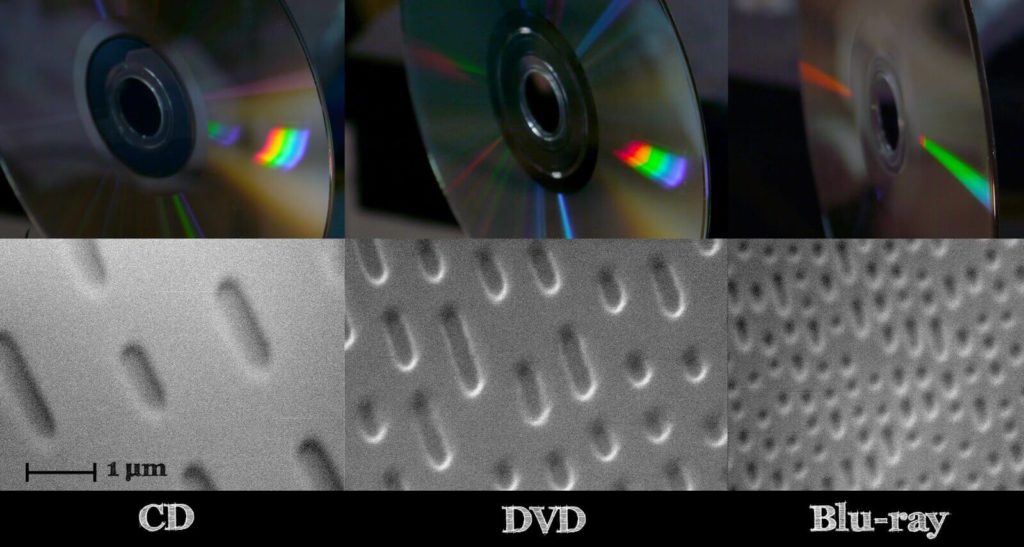
Использование кодирования позволяет извлекать информацию без потерь даже с поврежденного CD/DVD диска, когда какая либо область становится недоступной для считывания.
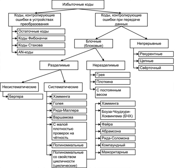
В зависимости от того, используется в системе обнаружение или исправление ошибок с помощью помехоустойчивого кода, различают следующие варианты:
- запрос повторной передачи (Automatic Repeat reQuest, ARQ): с помощью помехоустойчивого кода выполняется только обнаружение ошибок, при их наличии производится запрос на повторную передачу пакета данных;
- прямое исправление ошибок (Forward Error Correction, FEC): производится декодирование помехоустойчивого кода, т. е. исправление ошибок с его помощью.
Возможен также гибридный вариант, чтобы лишний раз не гонять информацию по каналу связи, например получили пакет информации, попробовали его исправить, и если не смогли исправить, тогда отправляется запрос на повторную передачу.
Исправление ошибок в помехоустойчивом кодировании
Любое помехоустойчивое кодирование добавляет избыточность, за счет чего и появляется возможность восстановить информацию при частичной потере данных в канале связи (носителе информации при хранении). В случае эффективного кодирования убирали избыточность, а в помехоустойчивом кодировании добавляется контролируемая избыточность.
Простейший пример – мажоритарный метод, он же многократная передача, в котором один символ передается многократно, а на приемной стороне принимается решение о том символе, количество которых больше.
Допустим есть 4 символа информации, А, B, С,D, и эту информацию повторяем несколько раз. В процессе передачи информации по каналу связи, где-то возникла ошибка. Есть три пакета (A1B1C1D1|A2B2C2D2|A3B3C3D3), которые должны нести одну и ту же информацию.

Но из картинки справа, видно, что второй символ (B1 и C1) они отличаются друг от друга, хотя должны были быть одинаковыми. То что они отличаются, говорит о том, что есть ошибка.
Необходимо найти ошибку с помощью голосования, каких символов больше, символов В или символов С? Явно символов В больше, чем символов С, соответственно принимаем решение, что передавался символ В, а символ С ошибочный.
Для исправления ошибок нужно, как минимум 3 пакета информации, для обнаружения, как минимум 2 пакета информации.
Параметры помехоустойчивого кодирования
Первый параметр, скорость кода R характеризует долю информационных («полезных») данных в сообщении и определяется выражением: R=k/n=k/m+k
- где n – количество символов закодированного сообщения (результата кодирования);
- m – количество проверочных символов, добавляемых при кодировании;
- k – количество информационных символов.
Параметры n и k часто приводят вместе с наименованием кода для его однозначной идентификации. Например, код Хэмминга (7,4) значит, что на вход кодера приходит 4 символа, на выходе 7 символов, Рида-Соломона (15, 11) и т.д.
Второй параметр, кратность обнаруживаемых ошибок – количество ошибочных символов, которые код может обнаружить.
Третий параметр, кратность исправляемых ошибок – количество ошибочных символов, которые код может исправить (обозначается буквой t).
Контроль чётности
Самый простой метод помехоустойчивого кодирования это добавление одного бита четности. Есть некое информационное сообщение, состоящее из 8 бит, добавим девятый бит.
Если нечетное количество единиц, добавляем 0.
1 0 1 0 0 1 0 0 | 0
Если четное количество единиц, добавляем 1.
1 1 0 1 0 1 0 0 | 1
Если принятый бит чётности не совпадает с рассчитанным битом чётности, то считается, что произошла ошибка.
1 1 0 0 0 1 0 0 | 1
Под кратностью понимается, всевозможные ошибки, которые можно обнаружить. В этом случае, кратность исправляемых ошибок 0, так как мы не можем исправить ошибки, а кратность обнаруживаемых 1.
Есть последовательность 0 и 1, и из этой последовательности составим прямоугольную матрицу размера 4 на 4. Затем для каждой строки и столбца посчитаем бит четности.
Прямоугольный код – код с контролем четности, позволяющий исправить одну ошибку:

И если в процессе передачи информации допустим ошибку (ошибка нолик вместо единицы, желтым цветом), начинаем делать проверку. Нашли ошибку во втором столбце, третьей строке по координатам. Чтобы исправить ошибку, просто инвертируем 1 в 0, тем самым ошибка исправляется.
Этот прямоугольный код исправляет все одно-битные ошибки, но не все двух-битные и трех-битные.
Рассчитаем скорость кода для:
- 1 1 0 0 0 1 0 0 | 1
Здесь R=8/9=0,88
- И для прямоугольного кода:
Здесь R=16/24=0,66 (картинка выше, двадцать пятую единичку (бит четности) не учитываем)
Более эффективный с точки зрения скорости является первый вариант, но зато мы не можем с помощью него исправлять ошибки, а с помощью прямоугольного кода можно. Сейчас на практике прямоугольный код не используется, но логика работы многих помехоустойчивых кодов основана именно на прямоугольном коде.
Классификация помехоустойчивых кодов
- Непрерывные — процесс кодирования и декодирования носит непрерывный характер. Сверточный код является частным случаем непрерывного кода. На вход кодера поступил один символ, соответственно, появилось несколько на выходе, т.е. на каждый входной символ формируется несколько выходных, так как добавляется избыточность.
- Блочные (Блоковые) — процесс кодирования и декодирования осуществляется по блокам. С точки зрения понимания работы, блочный код проще, разбиваем код на блоки и каждый блок кодируется в отдельности.
По используемому алфавиту:
- Двоичные. Оперируют битами.
- Не двоичные (код Рида-Соломона). Оперируют более размерными символами. Если изначально информация двоичная, нужно эти биты превратить в символы. Например, есть последовательность 110 110 010 100 и нужно их преобразовать из двоичных символов в не двоичные, берем группы по 3 бита — это будет один символ, 6, 6, 2, 4 — с этими не двоичными символами работают не двоичные помехоустойчивые коды.
Блочные коды делятся на
- Систематические — отдельно не измененные информационные символы, отдельно проверочные символы. Если на входе кодера присутствует блок из k символов, и в процессе кодирования сформировали еще какое-то количество проверочных символов и проверочные символы ставим рядом к информационным в конец или в начало. Выходной блок на выходе кодера будет состоять из информационных символов и проверочных.
- Несистематические — символы исходного сообщения в явном виде не присутствуют. На вход пришел блок k, на выходе получили блок размером n, блок на выходе кодера не будет содержать в себе исходных данных.
В случае систематических кодов, выходной блок в явном виде содержит в себе, то что пришло на вход, а в случае несистематического кода, глядя на выходной блок нельзя понять что было на входе.

Смотря на картинку выше, код 1 1 0 0 0 1 0 0 | 1 является систематическим, на вход поступило 8 бит, а на выходе кодера 9 бит, которые в явном виде содержат в себе 8 бит информационных и один проверочный.
Код Хэмминга
Код Хэмминга — наиболее известный из первых самоконтролирующихся и самокорректирующихся кодов. Позволяет устранить одну ошибку и находить двойную.

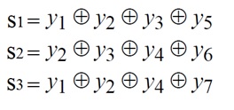
Код Хэмминга (7,4) — 4 бита на входе кодера и 7 на выходе, следовательно 3 проверочных бита. С 1 по 4 информационные биты, с 6 по 7 проверочные (см. табл. выше). Пятый проверочный бит y5, это сумма по модулю два 1-3 информационных бит. Сумма по модулю 2 это вычисление бита чётности.
Декодирование кода Хэмминга
Декодирование происходит через вычисление синдрома по выражениям:
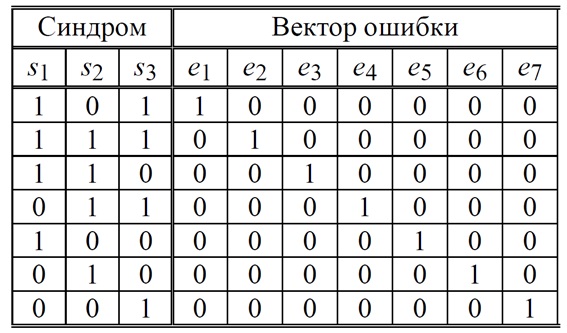
Синдром это сложение бит по модулю два. Если синдром не нулевой, то исправление ошибки происходит по таблице декодирования:
Расстояние Хэмминга
Расстояние Хэмминга — число позиций, в которых соответствующие символы двух кодовых слов одинаковой длины различны. Если рассматривать два кодовых слова, (пример на картинке ниже, 1 0 1 1 0 0 1 и 1 0 0 1 1 0 1) видно что они отличаются друг от друга на два символа, соответственно расстояние Хэмминга равно 2.
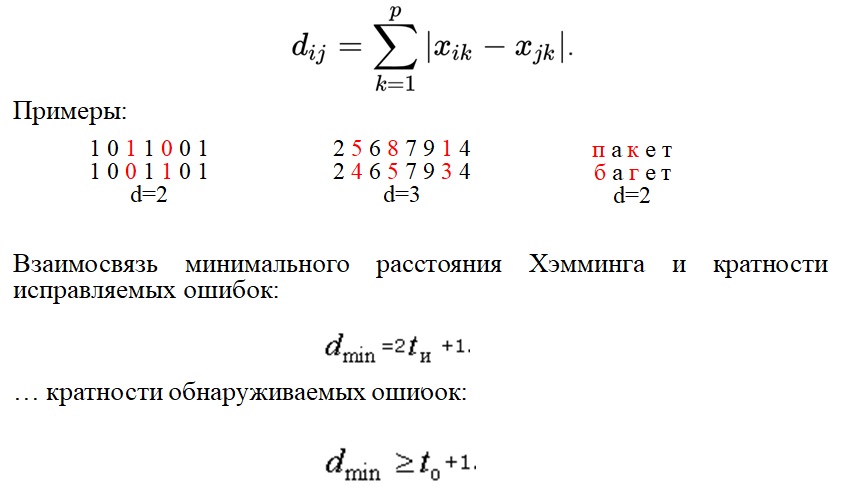
Кратность исправляемых ошибок и обнаруживаемых, связано минимальным расстоянием Хэмминга. Любой помехоустойчивый код добавляет избыточность с целью увеличить минимальное расстояние Хэмминга. Именно минимальное расстояние Хэмминга определяет помехоустойчивость.
Помехоустойчивые коды
Современные коды более эффективны по сравнению с рассматриваемыми примерами. В таблице ниже приведены Коды Боуза-Чоудхури-Хоквингема (БЧХ)
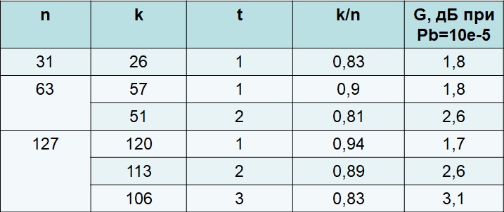
Из таблицы видим, что там один класс кода БЧХ, но разные параметры n и k.
- n — количество символов на входе.
- k — количество символов на выходе.
- t — кратность исправляемых ошибок.
- Отношение k/n — скорость кода.
- G (энергетический выигрыш) — величина, показывающая на сколько можно уменьшить отношение сигнал/шум (Eb/No) для обеспечения заданной вероятности ошибки.
Несмотря на то, что скорость кода близка, количество исправляемых ошибок может быть разное. Количество исправляемых ошибок зависит от той избыточности, которую добавим и от размера блока. Чем больше блок, тем больше ошибок он исправляет, даже при той же самой избыточности.
Пример: помехоустойчивые коды и двоичная фазовая манипуляция (2-ФМн). На графике зависимость отношения сигнал шум (Eb/No) от вероятности ошибки. За счет применения помехоустойчивых кодов улучшается помехоустойчивость.
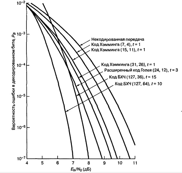
Из графика видим, код Хэмминга (7,4) на сколько увеличилась помехоустойчивость? Всего на пол Дб это мало, если применить код БЧХ (127, 64) выиграем порядка 4 дБ, это хороший показатель.
Компромиссы при использовании помехоустойчивых кодов
Чем расплачиваемся за помехоустойчивые коды? Добавили избыточность, соответственно эту избыточность тоже нужно передавать. Нужно: увеличивать пропускную способность канала связи, либо увеличивать длительность передачи.
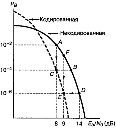
Компромисс:
- Достоверность vs полоса пропускания.
- Мощность vs полоса пропускания.
- Скорость передачи данных vs полоса пропускания
Необходимость чередования (перемежения)
Все помехоустойчивые коды могут исправлять только ограниченное количество ошибок t. Однако в реальных системах связи часто возникают ситуации сгруппированных ошибок, когда в течение непродолжительного времени количество ошибок превышает t.
Например, в канале связи шумов мало, все передается хорошо, ошибки возникают редко, но вдруг возникла импульсная помеха или замирания, которые повредили на некоторое время процесс передачи, и потерялся большой кусок информации. В среднем на блок приходится одна, две ошибки, а в нашем примере потерялся целый блок, включая информационные и проверочные биты. Сможет ли помехоустойчивый код исправить такую ошибку? Эта проблема решаема за счет перемежения.
Пример блочного перемежения:

На картинке, всего 5 блоков (с 1 по 25). Код работает исправляя ошибки в рамках одного блока (если в одном блоке 1 ошибка, код его исправит, а если две то нет). В канал связи отдается информация не последовательно, а в перемешку. На выходе кодера сформировались 5 блоков и эти 5 блоков будем отдавать не по очереди а в перемешку. Записали всё по строкам, но считывать будем, чтобы отправлять в канал связи, по столбцам. Информация в блоках перемешалась. В канале связи возникла ошибка и мы потеряли большой кусок. В процессе приема, мы опять составляем таблицу, записываем по столбцам, но считываем по строкам. За счет того, что мы перемешали большое количество блоков между собой, групповая ошибка равномерно распределится по блокам.
Помехоустойчивое кодирование. Часть 1: код Хэмминга +33
Программирование
Рекомендация: подборка платных и бесплатных курсов дизайна интерьера — https://katalog-kursov.ru/

Код Хэмминга – не цель этой статьи. Я лишь хочу на его примере познакомить вас с самими принципами кодирования. Но здесь не будет строгих определений, математических формулировок и т.д. Эта просто неплохой трамплин для понимания более сложных блочных кодов.
Самый, пожалуй, известный код Хэмминга (7,4). Что значат эти цифры? Вторая – число бит информационного слова — то, что мы хотим передать в целости и сохранности. А первое – размер кодового слова: информация удобренная избыточностью. Кстати термины «информационное слово» и «кодовое слово», употребляются во всех 7-ми книгах по теории помехоустойчивого кодирования, которые мне довелось бегло пролистать.

Такой код исправляет 1 ошибку. И не важно где она возникла. Избыточность несёт в себе 3 бита информации, этого достаточно, чтобы указать на одно из 7 положений ошибки или показать, что её нет. То есть ровно 8 вариантов ответов мы ждём. А 8 = 2^3, вот как всё совпало.
Чтобы получить кодовое слово, нужно информационное слово представить в виде полинома и умножить его на порождающий полином g(x). Любое число, переведя в двоичный вид, можно представить в виде полинома. Это может показаться странным и у не подготовленного читателя сразу встаёт только один вопрос «да зачем же так усложнять?». Уверяю вас, он отпадёт сам собой, когда мы получим первые результаты.
К примеру информационное слово 1010, значение каждого его разряда это коэффициент в полиноме:

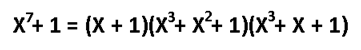
Во многих книгах пишут наоборот x+x^3. Не поддавайтесь на провокацию, это вносит только путаницу, ведь в записи числа 2-ичного, 16-ричного, младшие разряды идут справа, и сдвиги мы делаем влево/вправо ориентируясь на это. А теперь давайте умножим этот полином на порождающий полином. Порождающий полином специально для Хэмминга (7,4), встречайте: g(x)=x^3+x+1. Откуда он взялся? Ну пока считайте что он дан человечеству свыше, богами (объясню позже).

Если нужно складывать коэффициенты, то делаем по модулю 2: операция сложения заменяется на логическое исключающее или (XOR), то есть x^4+x^4=0. И в конечном итоге результат перемножения как видите из 4х членов. В двоичном виде это 1001110. Итак, получили кодовое слово, которое будем передавать на сторону по зашумлённому каналу. Замете, что перемножив информационное слово (1010) на порождающий полином (1011) как обычные числа – получим другой результат 1101110. Этого нам не надо, требуется именно «полиномиальное» перемножение. Программная реализация такого умножения очень простая. Нам потребуется 2 операции XOR и 2 сдвига влево (1й из которых на один разряд, второй на два, в соответствии с g(x)=1011):

Давайте теперь специально внесём ошибку в полученное кодовое слово. Например в 3-й разряд. Получиться повреждённое слово: 1000110.
Как расшифровать сообщение и исправить ошибку? Разумеется надо «полиномиально» разделить кодовое слово на g(x). Тут я уже не буду писать иксы. Помните что вычитание по модулю 2 — это то же самое что сложение, что в свою очередь, тоже самое что исключающее или. Поехали:

В программной реализации опять же ничего сверх сложного. Делитель (1011) сдвигаем влево до самого конца на 3 разряда. И начинаем удалять (не без помощи XOR) самые левые единицы в делимом (100110), на его младшие разряды даже не смотрим. Делимое поэтапно уменьшается 100110 -> 0011110 -> 0001000 -> 0000011, когда в 4м и левее разрядах не остаётся единиц, мы останавливаемся.
Нацело разделить не получилось, значит у нас есть ошибка (ну конечно же). Результат деления в таком случае нам без надобности. Остаток от деления является синдром, его размер равен размеру избыточности, поэтому мы дописали там ноль. В данном случае содержание синдрома нам никак не помогает найти местоположение повреждения. А жаль. Но если мы возьмём любое другое информационное слово, к примеру 1100. Точно так же перемножим его на g(x), получим 1110100, внесём ошибку в тот же самый разряд 1111100. Разделим на g(x) и получим в остатке тот же самый синдром 011. И я гарантирую вам, что к такому синдрому мы придём в обще для всех кодовых слов с ошибкой в 3-м разряде. Вывод напрашивается сам собой: можно составить таблицу синдромов для всех 7 ошибок, делая каждую из них специально и считая синдром.

В результате собираем список синдромов, и то на какую болезнь он указывает:

Теперь у нас всё есть. Нашли синдром, исправили ошибку, ещё раз поделили в данном случае 1001110 на 1011 и получили в частном наше долгожданное информационное слово 1010. В остатке после исправления уже будет 000. Таблица синдромов имеет право на жизнь в случае маленьких кодов. Но для кодов, исправляющих несколько ошибок – там список синдромов разрастается как чума. Поэтому рассмотрим метод «вылавливания ошибок» не имея на руках таблицы.
Внимательный читатель заметит, что первые 3 синдрома вполне однозначно указывают на положение ошибки. Это касается только тех синдромов, где одна единица. Кол-во единиц в синдроме называют его «весом». Опять вернёмся к злосчастной ошибке в 3м разряде. Там, как вы помните был синдром 011, его вес 2, нам не повезло. Сделаем финт ушами — циклический сдвиг кодового слова вправо. Остаток от деления 0100011 / 1011 будет равен 100, это «хороший синдром», указывает что ошибка во втором разряде. Но поскольку мы сделали один сдвиг, значит и ошибка сдвинулась на 1. Вот собственно и вся хитрость. Даже в случае жуткого невезения, когда ошибка в 6м разряде, вы, обливаясь потом, после 3 мучительных делений, но всё таки находите ошибку – это победа, лишь потому, что вы не использовали таблицу синдромов.
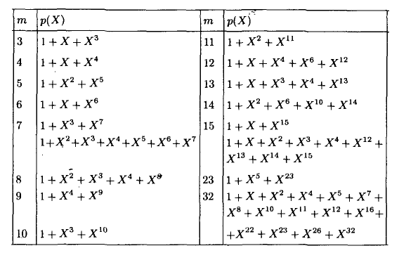
А как насчёт других кодов Хэмминга? Я бы сказал кодов Хэмминга бесконечное множество: (7,4), (15,11), (31,26),… (2^m-1, 2^m-1-m). Размер избыточности – m. Все они исправляют 1 ошибку, с ростом информационного слова растёт избыточность. Помехоустойчивость слабеет, но в случае слабых помех код весьма экономный. Ну ладно, а как мне найти порождающую функцию например для (15,11)? Резонный вопрос. Есть теорема, гласящая: порождающий многочлен циклического кода g(x) делит (x^n+1) без остатка. Где n – нашем случае размер кодового слова. Кроме того порождающий полином должен быть простым (делиться только на 1 и на самого себя без остатка), а его степень равна размеру избыточности. Можно показать, что для Хэмминга (7,4):
Этот код имеет целых 2 порождающих полинома. Не будет ошибкой использовать любой из них. Для остальных «хэммингов» используйте вот эту таблицу примитивных полиномов:
Соответственно для (15,11) порождающий многочлен g(x)=x^4+x+1. Ну а теперь переходим к десерту – к матрицам. С этого обычно начинают, но мы этим закончим. Для начала преобразую g(x) в матрицу, на которую можно умножить информационное слово, получив кодовое слово. Если g = 1011, то:
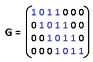
Называют её «порождающей матрицей». Дадим обозначение информационному слову d = 1010, а кодовое обозначим k, тогда:

Это довольно изящная формулировка. По быстродействию ещё быстрее, чем перемножение полиномов. Там нужно было делать сдвиги, а тут уже всё сдвинуто. Вектор d указывает нам: какие строки брать в расчёт. Самая нижняя строка матрицы – нулевая, строки нумеруются снизу вверх. Да, да, всё потому что младшие разряды располагаются справа и от этого никуда не деться. Так как d=1010, то я беру 1ю и 3ю строки, произвожу над ними операцию XOR и вуаля. Но это ещё не всё, приготовьтесь удивляться, существует ещё проверочная матрица H. Теперь перемножением вектора на матрицу мы можем получить синдром и никаких делений полиномов делать не надо.

Посмотрите на проверочную матрицу и на список синдромов, который получили выше. Это ответ на вопрос откуда берётся эта матрица. Здесь я как обычно подпортил кодовое слово в 3м разряде, и получил тот самый синдром. Поскольку сама матрица – это и есть список синдромов, то мы тут же находим положение ошибки. Но в кодах, исправляющие несколько ошибок, такой метод не прокатит. Придётся вылавливать ошибки по методу, описанному выше.
Чтобы лучше понять саму природу исправления ошибок, сгенерируем в обще все 16 кодовых слов, ведь информационное слово состоит всего из 4х бит:

Посмотрите внимательно на кодовые слова, все они, отличаются друг от друга хотя бы на 3 бита. К примеру возьмёте слово 1011000, измените в нём любой бит, скажем первый, получиться 1011010. Вы не найдёте более на него похожего слова, чем 1011000. Как видите для формирования кодового слова не обязательно производить вычисления, достаточно иметь эту таблицу в памяти, если она мала. Показанное различие в 3 бита — называется минимальное «хэммингово расстояние», оно является характеристикой блокового кода, по нему судят сколько ошибок можно исправить, а именно (d-1)/2. В более общем виде код Хэмминга можно записать так (7,4,3). Отмечу только, что Хэммингово расстояние не является разностью между размерами кодового и информационного слов. Код Голея (23,12,7) исправляет 3 ошибки. Код (48, 36, 5) использовался в сотовой связи с временным разделением каналов (стандарт IS-54). Для кодов Рида-Соломона применима та же запись, но это уже недвоичные коды.
Список используемой литературы:
1. М. Вернер. Основы кодирования (Мир программирования) — 2004
2. Р. Морелос-Сарагоса. Искусство помехоустойчивого кодирования (Мир связи) — 2006
3. Р. Блейхут. Теория и практика кодов, контролирующих ошибки — 1986
Число обнаруживаемых или исправляемых ошибок.
При применении двоичных кодов учитывают
только дискретные искажения, при которых
единица переходит в нуль (1 → 0) или нуль
переходит в единицу (0 → 1). Переход 1 →
0 или 0 → 1 только в одном элементе кодовой
комбинации называют единичной ошибкой
(единичным искажением). В общем случае
под кратностью ошибки подразумевают
число позиций кодовой комбинации, на
которых под действием помехи одни
символы оказались заменёнными на другие.
Возможны двукратные (t= 2) и многократные (t> 2) искажения элементов в кодовой
комбинации в пределах 0 <t<n.
Минимальное кодовое расстояние является
основным параметром, характеризующим
корректирующие способности данного
кода. Если код используется только для
обнаружения ошибок кратностью t0,
то необходимо и достаточно, чтобы
минимальное кодовое расстояние было
равно
dmin
> t0
+ 1. (13.10)
В этом случае никакая комбинация из t0ошибок не может перевести одну разрешённую
кодовую комбинацию в другую разрешённую.
Таким образом, условие обнаружения всех
ошибок кратностьюt0можно записать в виде:
t0≤ dmin — 1. (13.11)
Чтобы можно было исправить все ошибки
кратностью tии менее, необходимо иметь минимальное
расстояние, удовлетворяющее условию:
![]() . (13.12)
. (13.12)
В этом случае любая кодовая комбинация
с числом ошибок tиотличается от каждой разрешённой
комбинации не менее чем вtи+ 1 позициях. Если условие (13.12) не выполнено,
возможен случай, когда ошибки кратностиtисказят переданную
комбинацию так, что она станет ближе к
одной из разрешённых комбинаций, чем к
переданной или даже перейдёт в другую
разрешённую комбинацию. В соответствии
с этим, условие исправления всех ошибок
кратностью не болееtиможно записать в виде:
tи
≤(dmin
— 1) / 2 . (13.13)
Из (13.10) и (13.12) следует, что если код
исправляет все ошибки кратностью tи,
то число ошибок, которые он может
обнаружить, равноt0= 2∙tи. Следует
отметить, что соотношения (13.10) и (13.12)
устанавливают лишь гарантированное
минимальное число обнаруживаемых или
исправляемых ошибок при заданномdminи не ограничивают возможность обнаружения
ошибок большей кратности. Например,
простейший код с проверкой на чётность
сdmin= 2 позволяет обнаруживать не только
одиночные ошибки, но и любое нечётное
число ошибок в пределахt0<n.
Корректирующие возможности кодов.
Вопрос о минимально необходимой
избыточности, при которой код обладает
нужными корректирующими свойствами,
является одним из важнейших в теории
кодирования. Этот вопрос до сих пор не
получил полного решения. В настоящее
время получен лишь ряд верхних и нижних
оценок (границ), которые устанавливают
связь между максимально возможным
минимальным расстоянием корректирующего
кода и его избыточностью.
Так, граница Плоткинадаёт верхнюю
границу кодового расстоянияdminпри заданном числе разрядовnв
кодовой комбинации и числе информационных
разрядовm, и для
двоичных кодов:
![]() (13.14)
(13.14)
или
![]() при
при![]() . (13.15)
. (13.15)
Верхняя граница Хеммингаустанавливает
максимально возможное число разрешённых
кодовых комбинаций (2m)
любого помехоустойчивого кода при
заданных значенияхnиdmin:
 , (13.16)
где
![]() —
—
число сочетаний изnэлементов поiэлементам.
Отсюда можно получить выражение для
оценки числа проверочных символов:
 . (13.17)
Для значений (dmin/n)
≤ 0,3 разница между границей Хемминга и
границей Плоткина сравнительно невелика.
Граница Варшамова-Гильбертадля
больших значенийnопределяет нижнюю
границу для числа проверочных разрядов,
необходимого для обеспечения заданного
кодового расстояния:
 . (13.18)
Отметим, что для некоторых частных
случаев Хемминг получил простые
соотношения, позволяющие определить
необходимое число проверочных символов:
![]() дляdmin= 3,
дляdmin= 3,
![]() дляdmin= 4.
дляdmin= 4.
Блочные коды с dmin= 3 и 4 в литературе обычно называют кодами
Хемминга.
Все приведенные выше оценки дают
представление о верхней границе числаdminпри фиксированных значенияхnиmили оценку снизу числа проверочных
символовkпри заданныхmиdmin.
Существующие методы построения избыточных
кодов решают в основном задачу нахождения
такого алгоритма кодирования и
декодирования, который позволял бы
наиболее просто построить и реализовать
код с заданным значением dmin.
Поэтому различные корректирующие коды
при одинаковыхdminсравниваются по сложности кодирующего
и декодирующего устройств. Этот критерий
является в ряде случаев определяющим
при выборе того или иного кода.
Соседние файлы в папке ЛБ_3
- #
- #
14.04.2015937 б70KodHemmig.m
- #
14.04.20150 б62ЛБ_3.exe
Избыточное кодирование (англ. redundant encoding) — вид кодирования, использующий избыточное количество информации с целью последующего контроля целостности данных при записи/воспроизведении информации или при её передаче по линиям связи.
| Определение: |
| Код определяет ошибок, если при передаче кодового слова, в котором ошибок, алгоритм декодирования скажет, что есть ошибка. |
| Определение: |
| Код исправляет ошибок, если при передаче кодового слова, в котором ошибок, алгоритм декодирования сможет восстановить исходное слово. |
Код, определяющий одну ошибку
Увеличив объем кода на бит, можно получить возможность определять при передаче наличие одной ошибки. Для этого к коду нужно добавить бит : , такой, чтобы сумма всех единиц была четной. В случае, если контрольная сумма окажется нечетной, следует отправить запрос на повторную посылку элемента, в котором была обнаружена ошибка. Такое кодирование применяется только если вероятность ошибки крайне мала, например, в оперативной памяти компьютера.
Кодирование Хэмминга
Кодирование Хэмминга предусматривает как возможность обнаружения ошибки, так и возможность её исправления.
Рассмотрим простой пример — закодируем четыре бита: . Полученный код будет иметь длину бит и выглядеть следующим образом:
Рассмотрим табличную визуализацию кода:
Как видно из таблицы, даже если один из битов передался с ошибкой, содержащие его -суммы не сойдутся. Итого, зная строку и столбец в проиллюстрированной таблице можно точно исправить ошибочный бит. Если один из битов передался с ошибкой, то не сойдется только одна сумма и очевидно, что можно легко определить, какой бит неверный
По аналогичному принципу можно закодировать любое число бит. Пусть мы имеем исходную строку длиной в бит. Для получения её кода добавим к ней пар бит по следующему принципу:
- Первая пара: сумма четных бит и сумма нечетных бит
- Вторая пара: сумма тех бит, в чьем номере второй бит с конца ноль и сумма тех бит, в чьем номере второй бит с конца единица
…
- -тая пара: сумма тех бит, в чьем номере -тый бит с конца ноль и сумма тех бит, в чьем номере -тый бит с конца единица
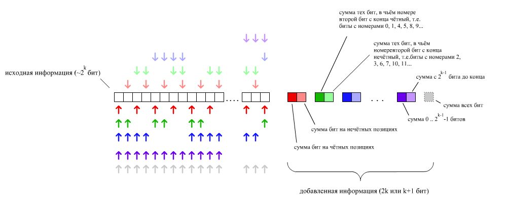
Соответствие добавленной информации исходным битам. Первый вариант кодирования соответствует использованию битов, раскрашенных в тёмные и светлые цвета, оптимизация — в тёмные цвета и серый
Легко понять, что если в одном бите из строки допущена ошибка, то с помощью дописанных пар бит можно точно определить, какой именно бит ошибочный. Это объясняется тем, что каждая пара определяет один бит номера ошибочного бита в строке. Всего пар , следовательно мы имеем бит номера ошибочного бита, что вполне достаточно: общее число бит строки не превосходит .
Теперь заметим, что в случае наличия ошибки в исходной строке, ровно один бит в каждой паре будет равен единице. Тогда можно оставить только один бит из пары. Однако этого будет недостаточно, поскольку если только один добавленный бит не соответствует строке, то нельзя понять, ошибка в нём или в строке. На этот случай можно добавить ещё один контрольный бит — всех битов строки.
Итого, увеличивая код длиной на , можно обнаружить и исправить одну ошибку.
См. также
- Обнаружение и исправление ошибок кодирования
Источники информации
- Wikipedia — Hamming code
Код Хэмминга
Содержание
- Самокорректирующийся код
- Алгоритм кодирования
- Самокорректирующийся код
- Результат работы программы
- Полученный мною опыт
Самокорректирующийся код
Код Хэ́мминга — наиболее известный из первых самоконтролирующихся и самокорректирующихся кодов. Построен применительно к двоичной системе счисления. Позволяет исправлять одиночную ошибку (ошибка в одном бите) и находить двойную.
Алгоритм кодирования
Предположим, что нужно сгенерировать код Хемминга для некоторого информационного кодового слова. В качестве примера возьмём 15-битовое кодовое слово x1…x15, хотя алгоритм пригоден для кодовых слов любой длины. В приведённой ниже таблице в первой строке даны номера позиций в кодовом слове, во второй — условное обозначение битов, в третьей — значения битов.
| 1 | 2 | 3 | 4 | 5 | 6 | 7 | 8 | 9 | 10 | 11 | 12 | 13 | 14 | 15 |
| x1 | x2 | x3 | x4 | x5 | x6 | x7 | x8 | x9 | x10 | x11 | x12 | x13 | x14 | x15 |
| 1 | 0 | 0 | 1 | 0 | 0 | 1 | 0 | 1 | 1 | 1 | 0 | 0 | 0 | 1 |
Вставим в информационное слово контрольные биты r0…r4 таким образом, чтобы номера их позиций представляли собой целые степени двойки: 1, 2, 4, 8, 16… Получим 20-разрядное слово с 15 информационными и 5 контрольными битами. Первоначально контрольные биты устанавливаем равными нулю. На рисунке контрольные биты выделены розовым цветом.
| 1 | 2 | 3 | 4 | 5 | 6 | 7 | 8 | 9 | 10 | 11 | 12 | 13 | 14 | 15 | 16 | 17 | 18 | 19 | 20 |
| r0 | r1 | x1 | r2 | x2 | x3 | x4 | r3 | x5 | x6 | x7 | x8 | x9 | x10 | x11 | r4 | x12 | x13 | x14 | x15 |
| 0 | 0 | 1 | 0 | 0 | 0 | 1 | 0 | 0 | 0 | 1 | 0 | 1 | 1 | 1 | 0 | 0 | 0 | 0 | 1 |
В общем случае количество контрольных бит в кодовом слове равно двоичному логарифму числа, на единицу большего, чем количество бит кодового слова (включая контрольные биты); логарифм округляется в большую сторону. Например, информационное слово длиной 1 бит требует двух контрольных разрядов, 2-, 3- или 4-битовое информационное слово — трёх, 5…11-битовое — четырёх, 12…26-битовое — пяти и т. д.
Добавим к таблице 5 строк (по количеству контрольных битов), в которые поместим матрицу преобразования. Каждая строка будет соответствовать одному контрольному биту (нулевой контрольный бит — верхняя строка, четвёртый — нижняя), каждый столбец — одному биту кодируемого слова. В каждом столбце матрицы преобразования поместим двоичный номер этого столбца, причём порядок следования битов будет обратный — младший бит расположим в верхней строке, старший — в нижней. Например, в третьем столбце матрицы будут стоять числа 11000, что соответствует двоичной записи числа три: 00011.
| 1 | 2 | 3 | 4 | 5 | 6 | 7 | 8 | 9 | 10 | 11 | 12 | 13 | 14 | 15 | 16 | 17 | 18 | 19 | 20 | ||
| r0 | r1 | x1 | r2 | x2 | x3 | x4 | r3 | x5 | x6 | x7 | x8 | x9 | x10 | x11 | r4 | x12 | x13 | x14 | x15 | ||
| 0 | 0 | 1 | 0 | 0 | 0 | 1 | 0 | 0 | 0 | 1 | 0 | 1 | 1 | 1 | 0 | 0 | 0 | 0 | 1 | ||
| 1 | 0 | 1 | 0 | 1 | 0 | 1 | 0 | 1 | 0 | 1 | 0 | 1 | 0 | 1 | 0 | 1 | 0 | 1 | 0 | r0 | |
| 0 | 1 | 1 | 0 | 0 | 1 | 1 | 0 | 0 | 1 | 1 | 0 | 0 | 1 | 1 | 0 | 0 | 1 | 1 | 0 | r1 | |
| 0 | 0 | 0 | 1 | 1 | 1 | 1 | 0 | 0 | 0 | 0 | 1 | 1 | 1 | 1 | 0 | 0 | 0 | 0 | 1 | r2 | |
| 0 | 0 | 0 | 0 | 0 | 0 | 0 | 1 | 1 | 1 | 1 | 1 | 1 | 1 | 1 | 0 | 0 | 0 | 0 | 0 | r3 | |
| 0 | 0 | 0 | 0 | 0 | 0 | 0 | 0 | 0 | 0 | 0 | 0 | 0 | 0 | 0 | 1 | 1 | 1 | 1 | 1 | r4 |
В правой части таблицы мы оставили пустым один столбец, в который поместим результаты вычислений контрольных битов. Вычисление контрольных битов производим следующим образом. Берём одну из строк матрицы преобразования (например, r0) и находим её скалярное произведение с кодовым словом, то есть перемножаем соответствующие биты обеих строк и находим сумму произведений. Если сумма получилась больше единицы, находим остаток от его деления на 2. Иными словами, мы подсчитываем сколько раз в кодовом слове и соответствующей строке матрицы в одинаковых позициях стоят единицы и берём это число по модулю 2.
Если описывать этот процесс в терминах матричной алгебры, то операция представляет собой перемножение матрицы преобразования на матрицу-столбец кодового слова, в результате чего получается матрица-столбец контрольных разрядов, которые нужно взять по модулю 2.
Например, для строки r0:
r0 = (1·0+0·0+1·1+0·0+1·0+0·0+1·1+0·0+1·0+0·0+1·1+0·0+1·1+0·1+1·1+0·0+1·0+0·0+1·0+0·1) mod 2 = 5 mod 2 = 1.
Полученные контрольные биты вставляем в кодовое слово вместо стоявших там ранее нулей. По аналогии находим проверочные биты в остальных строках. Кодирование по Хэммингу завершено. Полученное кодовое слово — 11110010001011110001.
| 1 | 2 | 3 | 4 | 5 | 6 | 7 | 8 | 9 | 10 | 11 | 12 | 13 | 14 | 15 | 16 | 17 | 18 | 19 | 20 | ||
| r0 | r1 | x1 | r2 | x2 | x3 | x4 | r3 | x5 | x6 | x7 | x8 | x9 | x10 | x11 | r4 | x12 | x13 | x14 | x15 | ||
| 0 | 0 | 1 | 0 | 0 | 0 | 1 | 0 | 0 | 0 | 1 | 0 | 1 | 1 | 1 | 0 | 0 | 0 | 0 | 1 | ||
| 1 | 0 | 1 | 0 | 1 | 0 | 1 | 0 | 1 | 0 | 1 | 0 | 1 | 0 | 1 | 0 | 1 | 0 | 1 | 0 | r0 | 1 |
| 0 | 1 | 1 | 0 | 0 | 1 | 1 | 0 | 0 | 1 | 1 | 0 | 0 | 1 | 1 | 0 | 0 | 1 | 1 | 0 | r1 | 1 |
| 0 | 0 | 0 | 1 | 1 | 1 | 1 | 0 | 0 | 0 | 0 | 1 | 1 | 1 | 1 | 0 | 0 | 0 | 0 | 1 | r2 | 1 |
| 0 | 0 | 0 | 0 | 0 | 0 | 0 | 1 | 1 | 1 | 1 | 1 | 1 | 1 | 1 | 0 | 0 | 0 | 0 | 0 | r3 | 0 |
| 0 | 0 | 0 | 0 | 0 | 0 | 0 | 0 | 0 | 0 | 0 | 0 | 0 | 0 | 0 | 1 | 1 | 1 | 1 | 1 | r4 | 1 |
Алгоритм декодирования
Алгоритм декодирования по Хэммингу абсолютно идентичен алгоритму кодирования. Матрица преобразования соответствующей размерности умножается на матрицу-столбец кодового слова и каждый элемент полученной матрицы-столбца берётся по модулю 2. Полученная матрица-столбец получила название «матрица синдромов». Легко проверить, что кодовое слово, сформированное в соответствии с алгоритмом, описанным в предыдущем разделе, всегда даёт нулевую матрицу синдромов.
Матрица синдромов становится ненулевой, если в результате ошибки (например, при передаче слова по линии связи с шумами) один из битов исходного слова изменил своё значение. Предположим для примера, что в кодовом слове, полученном в предыдущем разделе, шестой бит изменил своё значение с нуля на единицу (на рисунке обозначено красным цветом). Тогда получим следующую матрицу синдромов.
| 1 | 2 | 3 | 4 | 5 | 6 | 7 | 8 | 9 | 10 | 11 | 12 | 13 | 14 | 15 | 16 | 17 | 18 | 19 | 20 | ||
|---|---|---|---|---|---|---|---|---|---|---|---|---|---|---|---|---|---|---|---|---|---|
| r0 | r1 | x1 | r2 | x2 | x3 | x4 | r3 | x5 | x6 | x7 | x8 | x9 | x10 | x11 | r4 | x12 | x13 | x14 | x15 | ||
| 1 | 1 | 1 | 1 | 0 | 1 | 1 | 0 | 0 | 0 | 1 | 0 | 1 | 1 | 1 | 1 | 0 | 0 | 0 | 1 | ||
| 1 | 0 | 1 | 0 | 1 | 0 | 1 | 0 | 1 | 0 | 1 | 0 | 1 | 0 | 1 | 0 | 1 | 0 | 1 | 0 | s0 | 0 |
| 0 | 1 | 1 | 0 | 0 | 1 | 1 | 0 | 0 | 1 | 1 | 0 | 0 | 1 | 1 | 0 | 0 | 1 | 1 | 0 | s1 | 1 |
| 0 | 0 | 0 | 1 | 1 | 1 | 1 | 0 | 0 | 0 | 0 | 1 | 1 | 1 | 1 | 0 | 0 | 0 | 0 | 1 | s2 | 1 |
| 0 | 0 | 0 | 0 | 0 | 0 | 0 | 1 | 1 | 1 | 1 | 1 | 1 | 1 | 1 | 0 | 0 | 0 | 0 | 0 | s3 | 0 |
| 0 | 0 | 0 | 0 | 0 | 0 | 0 | 0 | 0 | 0 | 0 | 0 | 0 | 0 | 0 | 1 | 1 | 1 | 1 | 1 | s4 | 0 |
Заметим, что при однократной ошибке матрица синдромов всегда представляет собой двоичную запись (младший разряд в верхней строке) номера позиции, в которой произошла ошибка. В приведённом примере матрица синдромов (01100) соответствует двоичному числу 00110 или десятичному 6, откуда следует, что ошибка произошла в шестом бите.
Результат работы программы

Полученный мною опыт
- Работа с C#;
- Имею представление, что такое самокорректирующийся код;
- Изучил алгоритм кодирования и декодирования кодом Хэмминга;
- Работа с одномерными и двумерными массивами;
- Научился обрабатывать исключения с помощью do…while или try…catch.