The standard error of a regression slope is a way to measure the “uncertainty” in the estimate of a regression slope.
It is calculated as:

where:
- n: total sample size
- yi: actual value of response variable
- ŷi: predicted value of response variable
- xi: actual value of predictor variable
- x̄: mean value of predictor variable
The smaller the standard error, the lower the variability around the coefficient estimate for the regression slope.
The standard error of the regression slope will be displayed in a “standard error” column in the regression output of most statistical software:

The following examples show how to interpret the standard error of a regression slope in two different scenarios.
Example 1: Interpreting a Small Standard Error of a Regression Slope
Suppose a professor wants to understand the relationship between the number of hours studied and the final exam score received for students in his class.
He collects data for 25 students and creates the following scatterplot:

There is a clear positive association between the two variables. As hours studied increases, the exam score increases at a fairly predictable rate.
He then fits a simple linear regression model using hours studied as the predictor variable and final exam score as the response variable.
The following table shows the results of the regression:

The coefficient for the predictor variable ‘hours studied’ is 5.487. This tells us that each additional hour studied is associated with an average increase of 5.487 in exam score.
The standard error is 0.419, which is a measure of the variability around this estimate for the regression slope.
We can use this value to calculate the t-statistic for the predictor variable ‘hours studied’:
- t-statistic = coefficient estimate / standard error
- t-statistic = 5.487 / .419
- t-statistic = 13.112
The p-value that corresponds to this test statistic is 0.000, which indicates that ‘hours studied’ has a statistically significant relationship with final exam score.
Since the standard error of the regression slope was small relative to the coefficient estimate of the regression slope, the predictor variable was statistically significant.
Example 2: Interpreting a Large Standard Error of a Regression Slope
Suppose a different professor wants to understand the relationship between the number of hours studied and the final exam score received for students in her class.
She collects data for 25 students and creates the following scatterplot:

There appears to be slight positive association between the two variables. As hours studied increases, the exam score generally increases but not at a predictable rate.
Suppose the professor then fits a simple linear regression model using hours studied as the predictor variable and final exam score as the response variable.
The following table shows the results of the regression:

The coefficient for the predictor variable ‘hours studied’ is 1.7919. This tells us that each additional hour studied is associated with an average increase of 1.7919 in exam score.
The standard error is 1.0675, which is a measure of the variability around this estimate for the regression slope.
We can use this value to calculate the t-statistic for the predictor variable ‘hours studied’:
- t-statistic = coefficient estimate / standard error
- t-statistic = 1.7919 / 1.0675
- t-statistic = 1.678
The p-value that corresponds to this test statistic is 0.107. Since this p-value is not less than .05, this indicates that ‘hours studied’ does not have a statistically significant relationship with final exam score.
Since the standard error of the regression slope was large relative to the coefficient estimate of the regression slope, the predictor variable was not statistically significant.
Additional Resources
Introduction to Simple Linear Regression
Introduction to Multiple Linear Regression
How to Read and Interpret a Regression Table
SE of regression slope = sb1 = sqrt [ Σ(yi – ŷi)2 / (n – 2) ] / sqrt [ Σ(xi – x)2 ]. The equation looks a little ugly, but the secret is you won’t need to work the formula by hand on the test.
Contents
- 1 What is the standard error of the slope coefficient?
- 2 How do we calculate standard error?
- 3 How do you find standard error on a graph?
- 4 How do you calculate b0 and b1?
- 5 Is standard error the same as standard deviation?
- 6 How do I calculate standard error in Excel?
- 7 Why do we calculate standard error?
- 8 How do you calculate 95% CI?
- 9 What is the formula for standard error of regression?
- 10 How do you find slope from b1?
- 11 How do I calculate standard deviation?
- 12 How do you solve a regression equation?
- 13 How is standard error related to standard deviation?
- 14 How do you graph standard error in Excel?
- 15 How do you calculate standard error in a pivot table?
- 16 What is standard error example?
- 17 What is standard error test?
What is the standard error of the slope coefficient?
The standard error of the slope coefficient, Sb, indicates approximately how far the estimated slope, b (the regression coefficient computed from the sample), is from the population slope, β, due to the randomness of sampling.
How do we calculate standard error?
The standard error is calculated by dividing the standard deviation by the sample size’s square root. It gives the precision of a sample mean by including the sample-to-sample variability of the sample means.
How do you find standard error on a graph?
The standard error is calculated by dividing the standard deviation by the square root of number of measurements that make up the mean (often represented by N). In this case, 5 measurements were made (N = 5) so the standard deviation is divided by the square root of 5.
How do you calculate b0 and b1?
The mathematical formula of the linear regression can be written as y = b0 + b1*x + e , where: b0 and b1 are known as the regression beta coefficients or parameters: b0 is the intercept of the regression line; that is the predicted value when x = 0 . b1 is the slope of the regression line.
Is standard error the same as standard deviation?
The standard deviation (SD) measures the amount of variability, or dispersion, from the individual data values to the mean, while the standard error of the mean (SEM) measures how far the sample mean (average) of the data is likely to be from the true population mean.
How do I calculate standard error in Excel?
As you know, the Standard Error = Standard deviation / square root of total number of samples, therefore we can translate it to Excel formula as Standard Error = STDEV(sampling range)/SQRT(COUNT(sampling range)).
Why do we calculate standard error?
By calculating standard error, you can estimate how representative your sample is of your population and make valid conclusions. A high standard error shows that sample means are widely spread around the population mean—your sample may not closely represent your population.
How do you calculate 95% CI?
Calculating a C% confidence interval with the Normal approximation. ˉx±zs√n, where the value of z is appropriate for the confidence level. For a 95% confidence interval, we use z=1.96, while for a 90% confidence interval, for example, we use z=1.64.
What is the formula for standard error of regression?
Standard error of the regression = (SQRT(1 minus adjusted-R-squared)) x STDEV. S(Y). So, for models fitted to the same sample of the same dependent variable, adjusted R-squared always goes up when the standard error of the regression goes down.
How do you find slope from b1?
Regression from Summary Statistics. If you already know the summary statistics, you can calculate the equation of the regression line. The slope is b1 = r (st dev y)/(st dev x), or b1 = . 874 x 3.46 / 3.74 = 0.809.
How do I calculate standard deviation?
To calculate the standard deviation of those numbers:
- Work out the Mean (the simple average of the numbers)
- Then for each number: subtract the Mean and square the result.
- Then work out the mean of those squared differences.
- Take the square root of that and we are done!
How do you solve a regression equation?
The Linear Regression Equation
The equation has the form Y= a + bX, where Y is the dependent variable (that’s the variable that goes on the Y axis), X is the independent variable (i.e. it is plotted on the X axis), b is the slope of the line and a is the y-intercept.
How is standard error related to standard deviation?
The standard error of the sample mean depends on both the standard deviation and the sample size, by the simple relation SE = SD/√(sample size).
How do you graph standard error in Excel?
Add or remove error bars
- Click anywhere in the chart.
- Click the Chart Elements button. next to the chart, and then check the Error Bars box.
- To change the error amount shown, click the arrow next to Error Bars, and then pick an option.
How do you calculate standard error in a pivot table?
The standard error of the mean may be calculated by dividing the standard deviation by the square root of the number of values in the dataset. There is no direct function in MS Excel to get it automatically. Therefore, you must refer to its definition and type =STDEV(…)/SQRT(COUNT(…)) . )/SQRT(COUNT(A1:A100)) .
What is standard error example?
For example, if you measure the weight of a large sample of men, their weights could range from 125 to 300 pounds. However, if you look at the mean of the sample data, the samples will only vary by a few pounds. You can then use the standard error of the mean to determine how much the weight varies from the mean.
What is standard error test?
standard error of measurement (SEM), the standard deviation of error of measurement in a test or experiment. It is closely associated with the error variance, which indicates the amount of variability in a test administered to a group that is caused by measurement error.
To elaborate on Greg Snow’s answer: suppose your data is in the form of $t$ versus $y$ i.e. you have a vector of $t$’s $(t_1,t_2,…,t_n)^{top}$ as inputs, and corresponding scalar observations $(y_1,…,y_n)^{top}$.
We can model the linear regression as $Y_i sim N(mu_i, sigma^2)$ independently over i, where $mu_i = a t_i + b$ is the line of best fit. Greg’s way is to use vector notation.
We can rewrite the above in Greg’s notation: let
$Y = (Y_1,…,Y_n)^{top}$, $X = left( begin{array}{2} 1 & t_1\ 1 & t_2\ 1 & t_3\ vdots \ 1 & t_n end{array} right)$,
$beta = (a, b)^{top}$. Then the linear regression model becomes:
$Y sim N_n(Xbeta, sigma^2 I)$.
The goal then is to find the variance matrix of of the estimator $widehat{beta}$ of $beta$.
The estimator $widehat{beta}$ can be found by Maximum Likelihood estimation (i.e. minimise $||Y — Xbeta||^2$ with respect to the vector $beta$), and Greg quite rightly states that
$widehat{beta} = (X^{top}X)^{-1}X^{top}Y$.
See that the estimator $widehat{b}$ of the slope $b$ is just the 2nd component of $widehat{beta}$ — i.e $widehat{b} = widehat{beta}_2$
.
Note that $widehat{beta}$ is now expressed as some constant matrix multiplied by the random $Y$, and he uses a multivariate normal distribution result (see his 2nd sentence) to give you the distribution of $widehat{beta}$ as
$N_2(beta, sigma^2 (X^{top}X)^{-1})$.
The corollary of this is that the variance matrix of $widehat{beta}$ is $sigma^2 (X^{top}X)^{-1}$ and a further corollary is that the variance of $widehat{b}$ (i.e. the estimator of the slope) is $left[sigma^2 (X^{top}X)^{-1}right]_{22}$ i.e. the bottom right hand element of the variance matrix (recall that $beta := (a, b)^{top}$). I leave it as exercise to evaluate this answer.
Note that this answer $left[sigma^2 (X^{top}X)^{-1}right]_{22}$ depends on the unknown true variance $sigma^2$ and therefore from a statistics point of view, useless. However, we can attempt to estimate this variance by substituting $sigma^2$ with its estimate $widehat{sigma}^2$ (obtained via the Maximum Likelihood estimation earlier) i.e. the final answer to your question is $text{var} (widehat{beta}) approx left[widehat{sigma}^2 (X^{top}X)^{-1}right]_{22}$. As an exercise, I leave you to perform the minimisation to derive $widehat{sigma}^2 = ||Y — Xwidehat{beta}||^2$.
Just as a partial slope coefficient in a LARM can be interpreted as a measure of the magnitude of the effect of an independent variable, so too can the slope of a probability curve.
From: Encyclopedia of Social Measurement, 2005
Correlation and Regression
Andrew F. Siegel, Michael R. Wagner, in Practical Business Statistics (Eighth Edition), 2022
Standard Errors for the Slope and Intercept
You may suspect that there are standard errors lurking in the background because there are population parameters and sample estimators. Once you know the standard errors and degrees of freedom, you will be able to construct confidence intervals and hypothesis tests using the familiar methods of Chapters 9 and 10Chapter 10Chapter 9.
The standard error of the slope coefficient, Sb, indicates approximately how far the estimated slope, b (the regression coefficient computed from the sample), is from the population slope, β, due to the randomness of sampling. Note that Sb is a sample statistic. The formula for Sb is as follows:
Standard Error of the Regression Coefficient
Sb=SeSXn−1Degreesoffreedom=n−2
This formula says that the uncertainty in b is proportional to the basic uncertainty (Se) in the situation, but (1) Sb will be smaller when SX is large (because the line is better defined when the X values are more spread out) and (2) Sb will be smaller when the sample size n is large (because there is more information). It is common to see a term such as the square root of n in the denominator of a standard error formula, expressing the effect of additional information.
The degrees of freedom number for this standard error is n − 2, because two numbers, a and b, have been estimated to find the regression line.
For the production cost example (without the outlier!), the correlation is r = 0.869193, the sample size is n = 18, and the slope (variable cost) is b = 51.66 for the sample. The population is an idealized one: All of the weeks that might have happened under the same basic circumstances as the ones you observed. You might think of the population slope, β, as the slope you would compute if you had a lot more data. The standard error of b is
Sb=SeSXn−1=198.586.555218−1=198.5827.0278=7.35
The intercept term, a, was also estimated from the data. Therefore, it, too, has a standard error indicating its estimation uncertainty. The standard error of the intercept term, Sa, indicates approximately how far your estimate a is from α, the true population intercept term. This standard error, whose computation follows, also has n − 2 degrees of freedom and is a sample statistic:
Standard Error of the Intercept Term
Sa=Se1n+X¯2SX2(n−1)degreesoffreedom=n−2
This formula states that the uncertainty in a is proportional to the basic uncertainty (Se), that it is small when the sample size n is large, that it is large when X¯ is large (either positive or negative) with respect to SX (because the X data would be far from zero where the intercept is defined), and that there is a 1/n baseline term because a would be the average of Y if X¯ were zero.
For the production cost example, the intercept, a = $2272, indicates your estimated fixed costs. The standard error of this estimate is
Sa=Se1n+X¯2SX2(n−1)=198.58118+32.5026.55522(18−1)=198.580.0555556+1056.25730.50=198.581.5015=243.33
Read full chapter
URL:
https://www.sciencedirect.com/science/article/pii/B9780128200254000117
Probit/Logit and Other Binary Models
William D. Berry, in Encyclopedia of Social Measurement, 2005
The Meaning of Slope Coefficients in a Linear Probability Model
To understand the nature of the slope coefficient β in the LPM of Eq. (3), consider the conditional mean on the left side. Since Y can assume only the two values zero and one, the expected value of Y given the value of X is equal to 1 multiplied by “the probability that Y equals 1 given the value of X” plus 0 multiplied by “the probability that Y equals 0 given the value of X.” Symbolically,
(4)E(Y|X)=(1)[P(Y=1|X)]+(0)[P(Y=0|X)].
Of course, one multiplied by any value is that value, and zero multiplied by any number remains zero; so Eq. (4) simplifies to
(5)E(Y|X)=[P(Y=1|X)].
Given this equality, P(Y = 1∣X) can be substituted for E(Y∣X) in Eq. (3), obtaining
(6)P(Y=1|X)=α+βX.
This revised form of the PRF for the LPM—with the probability that Y equals 1 as the dependent variable—implies that the slope coefficient β indicates the change in the probability that Y equals 1 resulting from an increase of one in X.
In the more general LPM with multiple independent variables (say k of them—X1, X2,…, Xk), the PRF takes the form
E(Y|X1,X2,X3,…,Xk)=P(Y=1|X1,X2,X3,⋯,Xk)=α+β1X1+β2X2+β3X3+…+βkXk.
If (bold italicized) X is used as a shorthand for all the independent variables, this equation simplifies to
(7)E(Y|X)=P(Y=1|X)=α+β1X1+β2X2+β3X3+…+βkXk.
The slope coefficient, βi, for independent variable Xi (where i can be 1, 2, 3, …, k) can be interpreted as the change in the probability that Y equals 1 resulting from a unit increase in Xi when the remaining independent variables are held constant.
Read full chapter
URL:
https://www.sciencedirect.com/science/article/pii/B0123693985001766
Type I and Type II Error
Alesha E. Doan, in Encyclopedia of Social Measurement, 2005
The Alternative or Research Hypothesis
The alternative (also referred to as the research) hypothesis is the expectation a researcher is interested in investigating. Typically, the alternative hypothesis will naturally emerge from the particular area under investigation. An alternative hypothesis may, for example, test whether the slope coefficient (β) is not zero (Ha: β2 ≠ 0), or it may test whether a relationship exists between the dependent variable (Yi) and the independent variable (Xi). In this case, the alternative hypothesis is a two-sided hypothesis, indicating that the direction of the relationship is not known. Typically a two-sided hypothesis occurs when a researcher does not have sound a priori or theoretical expectations about the nature of the relationship. Conversely, in the presence of strong theory or a priori research, the alternative hypothesis can be specified according to a direction, in which case it takes on the following forms: Ha: β2 > 0 or Ha: β2 < 0.
Read full chapter
URL:
https://www.sciencedirect.com/science/article/pii/B0123693985001109
Correlation and Regression
Andrew F. Siegel, in Practical Business Statistics�(Sixth Edition), 2012
Other Methods of Testing the Significance of a Relationship
There are other methods for testing the significance of a relationship. Although they may appear different at first glance, they always give the same answer as the method just described, based on the regression coefficient. These alternate tests are based on other statistics—for example, the correlation, r, instead of the slope coefficient, b. But since the basic question is the same (is there a relationship or not?), the answers will be the same also. This can be mathematically proven.
There are two ways to perform the significance test based on the correlation coefficient. You could look up the correlation coefficient in a special table, or else you could transform the correlation coefficient to find the t statistic t=r(n−2)/(1−r2) to be compared to the t table value with n − 2 degrees of freedom. In the end, the methods yield the same answer as testing the slope coefficient. In fact, the t statistic defined from the correlation coefficient is the same number as the t statistic defined from the slope coefficient (t = b/ Sb).
This implies that you may conclude that there is significant correlation or that the correlation is not significant based on a test of significance of the regression coefficient, b. In fact, you may conclude that there is significant positive correlation if the relationship is significant and b > 0. Or, if the relationship is significant and b < 0, you may conclude that there is a significant negative correlation.
There is a significance test called the F test for overall significance of a regression relationship. This test will be covered in the next chapter, on multiple regression. Although this test may also look different at first, in the end it is the same as testing the slope coefficient when you have just X and Y as the only variables in the analysis.
Read full chapter
URL:
https://www.sciencedirect.com/science/article/pii/B9780123852083000110
Metric Predicted Variable with One Nominal Predictor
John K. Kruschke, in Doing Bayesian Data Analysis (Second Edition), 2015
19.4.3 Relation to hierarchical linear regression
The model in this section has similarities to the hierarchical linear regression of Section 17.3. In particular, Figure 17.5 (p. 492) bears a resemblance to Figure 19.5, in that different subsets of data are being fit with lines, and there is hierarchical structure across the subsets of data.
In Figure 17.5, a line was fit to data from each individual, while in Figure 19.5, a line was fit to data from each treatment. Thus, the nominal predictor in Figure 17.5 is individuals, while the nominal predictor in Figure 19.5 is groups. In either case, the nominal predictor affects the intercept term of the predicted value.
The main structural difference between the models is in the slope coefficients on the metric predictor. In the hierarchical linear regression of Section 17.3, each individual is provided with its own distinct slope, but the slopes of different individuals mutually informed each other via a higher-level distribution. In the model of Figure 19.5, all the groups are described using the same slope on the metric predictor. For a more detailed comparison of the model structures, compare the hierarchical diagrams in Figures 17.6 (p. 493) and 19.4 (p. 570).
Conceptually, the main difference between the models is merely the focus of attention. In the hierarchical linear regression model, the focus was on the slope coefficient. In that case, we were trying to estimate the magnitude of the slope, simultaneously for individuals and overall. The intercepts, which describe the levels of the nominal predictor, were of ancillary interest. In the present section, on the other hand, the focus of attention is reversed. We are most interested in the intercepts and their differences between groups, with the slopes on the covariate being of ancillary interest.
Read full chapter
URL:
https://www.sciencedirect.com/science/article/pii/B9780124058880000192
Aberration-Corrected Electron Microscopy
Maximilian Haider, … Stephan Uhlemann, in Advances in Imaging and Electron Physics, 2008
1 Fourth-Order Aberrations
For the fourth-order path deviation we find
(35)u(4)=α4uαααα+αα¯3uαααα¯.
This follows by substituting
u(3)=αuα+α¯2uαα¯+α2α¯uααα¯ in the iteration formula [Eq. (6)] after collecting the fourth-order terms. The image coefficients are
(36)Cαααα=∫3ηΨ3su¯αα¯2uαdz,
(37)Cαααα¯=∫6ηΨ3su¯ααα¯uα2dz.
The second coefficient can be evaluated further after inserting the explicit representation of the spherical aberration ray. We obtain by partial integration the relation
(38)Cαααα¯=4C¯αααα.
According to this result the three-lobe aberration at the image has the form
(39)u(4)/uγ=α4D4+4αα¯3D¯4.
Since Ψ3s is a symmetric function and uα is anti-symmetric, we find from Eq. (36) that the three-lobe aberration D4 = Cαααα vanishes at the imageplane but not the corresponding slope coefficient
(40)cαααα=−∫3ηΨ3su¯αα¯2uγdz.
As a direct effect the latter is visible as a threefold distortion at the diffraction plane. Residual three-lobe aberration shows up also at the image if the intermediate image plane is moved away from the mid-plane S0 of the corrector. For this reason focusing through the corrector should be avoided. To shift the position of an image plane (e.g., the SA plane below the corrector in CTEM) always excitation of the adapter lens should be changed; the objective lens should never be tuned. Also in STEM the probe semi-angle should be tuned by changing lenses above the corrector only.
From Eq. (40) we can calculate a SCOFF approximation for the slope coefficient of the three-lobe aberration
(41)cαααα=910η3Ψ3s3f03L6.
In Figure 34 the fourth-order aberration rays uαααα and uα
![]()
are plotted according to an exact calculation. Although the three-lobe aberration becomes complex-valued due to the influence of the transfer lenses, it is still point-corrected at the image. The contribution of the transfer lensesto D4 cancels by symmetry. It is important to note that inside the second hexapole the aberration ray uαααα ≈ f0cαααα is almost constant. The slope coefficient cαααα is affected by the third-order aberrations of the transfer lenses. Actually their residual field astigmatism FA3,TL makes the uαααα ray complex-valued. This effect can be estimated by considering an off-axial image point u = αf0 at plane S1 with slope u′ =
![]()
2A2/f0. At the conjugated plane S2 a path deviation is induced by the field astigmatism of the transfer lenses. The result adds to the aberration ray of the three-lobe aberration inside the second hexapole field

FIGURE 34. Fourth-order axial aberration ray uαααα = xαααα + iyαααα and coefficient function of the three-lobe aberration D4 = Cαααα for a CTEM with hexapole corrector.
(42)uαααα=−910η3Ψ3s3L6f04+3ηΨ3sLf04FA3,TL.
This effect is clearly visible in Figure 34. Although it is rather small, it has important consequence for the residual fifth-order aberrations.
At this stage, we can summarize that for a system equipped with a hexapole Cs corrector, no residual axial aberrations up to and including fourth order occur. The first nonvanishing axial aberrations of the hexapole corrector are of fifth order.
Read full chapter
URL:
https://www.sciencedirect.com/science/article/pii/S1076567008010021
Omitted Variable Bias
Paul A. Jargowsky, in Encyclopedia of Social Measurement, 2005
Appendix: Expectation of the Bivariate Slope Coefficient with an Omitted Variable
Assume that the true model is:
(14)Yi=β1+β2X2i+β3X3i+uiui∼N(0,σ2)
However, the following model is estimated:
(15)Yi=α1+α2X2+ɛi
For ease of presentation, let lower-case letters represent deviations from the respective means. In other words:
yi=Yi−Y¯x2i=X2i−X¯2x3i=X3i−X¯3.
It is also useful to note the following relation:
(16)∑x2iyi=∑x2i(Yi−Y¯)=∑x2iYi−Y¯∑x2i=∑x2iYi.
The second term disappears because the sum of deviations around a mean is always zero.
The expectation of the slope coefficient from the incorrect bivariate regression is:
(17)E[αˆ2]=E[∑x2iyi∑x2i2]=E[∑x2iYi∑x2i2].
As shown, for example, by Gujarati in 2003, the first step is the standard solution for the bivariate slope coefficient. In the second step, we make use of Eq. (16). Now we substitute the true model, Eq. (14), simplify the expression, and take the expectation:
(18)E[αˆ2]=E[∑x2i(β1+β2X2i+β3X3i+ui)∑x2i2]=E[β1∑x2i+β2∑x2iX2i+β3∑x2iX3i+∑x2iui∑x2i2]=E[0+β2+β3(∑x2ix3i∑x2i2)+∑x2iui∑x2i2]=β2+β3γ32.
This is the result noted in Eq. (4). The first term goes to zero because the sum of deviations around a mean is always zero, and the final term has an expectation of zero because the model assumes no covariance between the Xs and the disturbance term. The raw values of X2 and X3 are replaced by their deviations (x2 and x3) in the third step by making use of the property demonstrated in Eq. (16).
Read full chapter
URL:
https://www.sciencedirect.com/science/article/pii/B0123693985001274
Multilevel Analysis
Joop J. Hox, Cora J.M. Maas, in Encyclopedia of Social Measurement, 2005
Example of Multilevel Regression Analysis
Assume that we have data from school classes. On the pupil level, we have the outcome variable Popularity measured by a self-rating scale that ranges from 0 (very unpopular) to 10 (very popular). We have one explanatory variable Gender (0 = boy, 1 = girl) on the pupil level and one class level explanatory variable Teacher experience (in years). We have data from 2000 pupils from 100 classes, so the average class size is 20 pupils. The data are described and analyzed in more detail in Hox’s 2002 handbook.
Table I presents the parameter estimates and standard errors for a series of models. Model M0 is the null model, the intercept-only model. The intercept-only model estimates the intercept as 5.31, which is simply the weighted average popularity across all schools and pupils. The variance of the pupil-level residuals is estimated as 0.64. The variance of the class-level residuals is estimated as 0.87. The intercept estimate is much larger than the corresponding standard error, and the calculation of the Z test shows that it is significant at p < 0.005. As previously mentioned, the Z test is not optimal for testing variances. If the second-level variance term is restricted to zero, the deviance of the model goes up to 6489.5. The difference between the deviances is 1376.8, with one more parameter in the intercept-only model. The chi-square of 1376.8 with one degree of freedom is also significant at p < 0.005. The intraclass correlation is ρ=σu02/σu02+σe2=0.87/0.87+0.64=0.58. Thus, 58% of the variance of the popularity scores is at the group level, which is very high. Because the intercept-only model contains no explanatory variables, the variances terms represent unexplained residual variance.
Table I. Multilevel Models for Pupil Popularity
| Model | M0: Intercept-only | M1: +Pupil gender and Teacher experience | M2: +Cross-level interaction |
|---|---|---|---|
| Fixed part | |||
| Predictor | Coefficient (SE) | Coefficient (SE) | Coefficient (SE) |
| Intercept | 5.31 (0.10) | 3.34 (0.16) | 3.31 (0.16) |
| Pupil gender | 0.84 (0.06) | 1.33 (0.13) | |
| Teacher experience | 0.11 (0.01) | 0.11 (0.01) | |
| Pupil gender Teacher exprience | −0.03 (0.01) | ||
| Random part | |||
| σe2 | 0.64 (0.02) | 0.39 (0.01) | 0.39 (0.01) |
| σu02 | 0.87 (013) | 0.40 (0.06) | 0.40 (0.06) |
| σu12 | 0.27 (0.05) | 0.22 (0.04) | |
| σu012 | 0.02 (0.04) | 0.02 (0.04) | |
| Deviance | 5112.7 | 4261.2 | 4245.9 |
Model M1 predicts the outcome variable Popularity by the explanatory variables Gender and Teacher experience, with a random component for the regression coefficient of gender, and model M2 adds the cross-level interaction term between Gender and Teacher experience. We can view these models as built up in the following sequence of steps:
(8)Popularityij=β0j+β1jGenderij+eij
In this regression equation, β0j is the usual intercept, β1j is the usual regression coefficient (regression slope) for the explanatory variable gender, and eij is the usual residual term. The subscript j is for the classes (j = 1,…, J) and the subscript i is for individual pupils (i = 1,…, Nj). We assume that the intercepts β0j and the slopes β1j vary across classes.
In our example data, the model corresponding to Eq. (8) results in significant variance components at both levels (as determined by the deviance-difference test). In the next step, we hope to be able to explain at least some of this variation by introducing class-level variables. Generally, we will not be able to explain all the variation of the regression coefficients, and there will be some unexplained residual variation—hence the name random coefficient model, the regression coefficients (intercept and slopes) have some amount of (residual) random variation between groups. Variance component model refers to the statistical problem of estimating the amount of random variation. In our example, the specific value for the intercept and the slope coefficient for the pupil variable Gender are class characteristics. A class with a high intercept is predicted to have more popular pupils than a class with a low value for the intercept. Similarly, differences in the slope coefficient for gender indicate that the relationship between the pupils’ gender and their predicted popularity is not the same in all classes. Some classes may have a high value for the slope coefficient of gender; in these classes, the difference between boys and girls is relatively large. Other classes may have a low value for the slope coefficient of gender; in these classes, gender has a small effect on the popularity, which means that the difference between boys and girls is small.
The next step in the hierarchical regression model is to explain the variation of the regression coefficients β0j and β1j by introducing the explanatory variable Teacher experience at the class level. Model M1 models the intercept as follows:
(9)β0j=γ00+γ01Teacher experiencej+u0j
and model M2 models the slope as follows:
(10)β1j=γ10+γ11Teacher experiencej+u1j
Equation (9) predicts the average popularity in a class (the intercept β0j) by the teacher’s experience. Thus, if γ01 is positive, the average popularity is higher in classes with a more experienced teacher. Conversely, if γ01 is negative, the average popularity is lower in classes with a more experienced teacher. The interpretation of Eq. (10) is more complicated. Equation (10) states that the relationship, as expressed by the slope coefficient β1j, between the popularity and the gender of the pupil, depends on the amount of experience of the teacher. If γ11 is positive, the gender effect on popularity is larger with experienced teachers. On the other hand, if γ11 is negative, the gender effect on popularity is smaller with experienced teachers. Thus, the amount of experience of the teacher interacts with the relationship between popularity and gender; this relationship varies according to the value of the teacher experience.
The u terms u0j and u1j in Eqs. (9) and (10) are the residual terms at the class level. The variance of the residual u0j is denoted by σu02, and the variance of the residual u1j is denoted by σu12. The covariance between the residuals u0j and u1j is σu01, which is generally not assumed to be zero.
Our model with one pupil-level and one class-level explanatory variable including the cross-level interaction can be written as a single complex regression equation by substituting Eqs. (9) and (10) into Eq. (8). This produces:
(11)Popularityij=γ00+γ10Genderij+γ01Teacher experiencej+γ11×Teacher experiencej×Genderij+u1jGenderij+u0j+eij
Note that the result of modeling the slopes using the class-level variable implies adding an interaction term and second-level residuals u1j that are related to the pupil-level variable Gender. Model M2 is the most complete, including both available explanatory variables and the cross-level interaction term. The interaction term is significant using the Z test. Because we have used FML estimation, we can also test the interaction term by comparing the deviances of models M1 and M2. The deviance-difference is 15.3, which has a chi-square distribution with one degree of freedom and p < 0.005. Using a deviance-difference test on the second-level variance components in model M2, by restricting variance terms to zero and then comparing deviances, leads to the conclusion that all variance terms are significant and that the covariance term is not. This means, that not all residual variation in the intercept and slope can be modeled by the explanatory variables.
The interpretation of model M2 is straightforward. The regression coefficients for both explanatory variables are significant. The regression coefficient for pupil gender is 1.33. Because pupil gender is coded 0 = boy and 1 = girl, this means that on average the girls score 1.33 points higher on the popularity measure. The regression coefficient for teacher experience is 0.11, which means that for each year of experience of the teacher, the average popularity score of the class goes up with 0.11 points. Because there is an interaction term in the model, the effect of 1.33 for pupil gender is the expected effect for teachers with zero experience. The regression coefficient for the cross-level interaction is −0.03, which is small but significant. The negative value means that with experienced teachers, the advantage of being a girl is smaller than expected from the direct effects only. Thus, the difference between boys and girls is smaller with more experienced teachers. A comparison of the other results between the two models shows that the variance component for pupil gender goes down from 0.27 in the direct effects model (M1) to 0.22 in the cross-level model (M2). Hence, the cross-level model explains about 19% of the variation of the slopes for pupil gender.
The significant and quite large variance of the regression slopes for pupil gender implies that we should not interpret the estimated value of 1.33 without considering this variation. In an ordinary regression model, without multilevel structure, the value of 1.33 means that girls are expected to differ from boys by 1.33 points, for all pupils in all classes. In our multilevel model, the regression coefficient for pupil gender varies across the classes and the value of 1.33 is just the expected value across all classes (for teachers with zero experience). The variance of the slope is estimated in model M1 as 0.27. Model M2 shows that part of this variation can be explained by variation in teacher experience. The interpretation of the slope variation is easier when we consider their standard deviation, which is the square root of the variance, or 0.52 in our example data. The varying regression coefficients are assumed to follow a normal distribution. Thus, we may expect 95% of the regression slopes to lie between two standard deviations above or below their average. Given the estimated values of 1.33 (in model M2, for inexperienced teachers) or 0.84 (in model M1, average for all teachers) the vast majority of the classes are expected to have positive slopes for the effect of pupil gender. Figure 1 provides a graphical display of the slope variation, which confirms the conclusion that almost all class slopes are expected to be positive.

Figure 1. One hundred class slopes for pupil gender.
Read full chapter
URL:
https://www.sciencedirect.com/science/article/pii/B0123693985005600
Linear Regression
Ronald N. Forthofer, … Mike Hernandez, in Biostatistics (Second Edition), 2007
13.2.4 The Y-intercept
It is also possible to form confidence intervals and to test hypotheses about β0, although these are usually of less interest than those for β1. The location of the Y intercept is relatively unimportant compared to determining whether or not there is a relation between the dependent and independent variables. However, sometimes we wish to compare whether or not both our coefficients — slope and Y intercept — agree with those presented in the literature. In this case, we are interested in examining β0 as well as β1.
Since the estimator of β0 is also a linear combination of the observed values of the normally distributed dependent variable, βˆ0 also follows a normal distribution. The standard error of βˆ0 is estimated by
est.s.e.(β0)=sY|X∑xi2n∑(xi-x¯)2.
The hypothesis of interest is
H0:β0=β00
versus either a one- or two-sided alternative hypothesis. The test statistic for this hypothesis is
t=βˆ0=β00sY|X∑xi2/[n∑(xi-x¯)2]
and this is compared to ±tn−2,1−α/2 for the two-sided alternative hypothesis. If the alternative hypothesis is that β0 is greater than β00, we reject the null hypothesis in favor of the alternative when t is greater than tn−2,1−α. If the alternative hypothesis is that β0 is less than β00, we reject the null hypothesis in favor of the alternative when t is less than −tn−2,1−α.
The (1 − α/2)*100 percent confidence interval for β0 is given by
βˆ0±tn-2,1-α/2sY|X=∑xi2∑(xi-x¯)2.
Let us form the 99 percent confidence interval for β0 for these SBP data. The 0.995 value of the t distribution with 48 degrees of freedom is approximately 2.68. Therefore, the confidence interval is found from the following calculations
61.14±2.68(14.52)14231950(4506.5)=61.14±30.93
which gives an interval from 30.21 to 92.07, a wide interval.
Read full chapter
URL:
https://www.sciencedirect.com/science/article/pii/B9780123694928500182
Variational and the Optimal Control Models in Biokinetics
Adam Moroz, in The Common Extremalities in Biology and Physics (Second Edition), 2012
3.1.6 Some Conclusions
It has been illustrated above how Eq. (3.16) can be obtained by employing the optimal control/variational technique. It is coinciding in a form with the logistical differential equation (3.6). Initially, the variable u was the proportionality coefficient in the control equation (3.8). Finally, in the transformed equation (3.16), the control u linearly depends on ν and the coefficient n, which characterizes cooperativity. So, in this way, the artificially introduced control u in the kinetic equation (3.8) later “materializes” into a function of state variable (saturation) ν with a characteristic constant n that can be considered as cooperativity.
One shall note that with an increase of cooperativity n, the rigidity of the regulation also increases, which results in an increase in the slope coefficient in Eq. (3.16). Figures 3.1B and 3.3A illustrate this graphically and indicate that the binding and the binding control, expressed as its cooperativity, can be considered in terms of optimal control in an uncontradictory manner. It also means that the binding description can be formulated as an optimal control problem and also as a variational problem. This consequently suggests the methodology of the least action principle. The coefficient of inclination, which describes cooperativity, is related to the control amplitude—this also being the specific cost of control.
However, one can note that the consideration presented here was based on assumptions of an ideal cooperativity. A disadvantage with this consideration is the phenomenological appearance of the energetic cost/penalty function, which is dependent on the state variable—saturation. For other well-known cooperativity models—like Adair [46], Monod–Wyman–Changeux [47], and Koshland–Nemethy–Filmer [48]—the optimal control formulations certainly will be more sophisticated.
The methodology shown above demonstrates that the cooperative macroscopic binding behavior can be explained from the optimal control perspective by considering the elementary binding as an optimal energetical process. In some sense, it extends the understanding of the control process, particularly its evolution in adaptive systems. In mechanics, as we have seen, the formal introduction of the control by the rate allowed the optimal control formulation [67] when the control appears as a dummy-like variable. In contrast, in biological and biochemical kinetics, when considering the OC formulation of binding, the control variable u does not look like a dummy variable (see Figure 3.3B). The optimal control is involved in an optimal regulation loop, when the Hill cooperativity constant can be interpreted from the OC perspective, as the rigidity of control. The kinetic momentum (co-state variable) can be interpreted as an energetic-like partial penalty/price/cost of deviation from the optimal dynamic control.
Read full chapter
URL:
https://www.sciencedirect.com/science/article/pii/B9780123851871000034
In statistics, the parameters of a linear mathematical model can be determined from experimental data using a method called linear regression. This method estimates the parameters of an equation of the form y = mx + b (the standard equation for a line) using experimental data. However, as with most statistical models, the model will not exactly match the data; therefore, some parameters, such as the slope, will have some error (or uncertainty) associated with them. The standard error is one way of measuring this uncertainty and can be accomplished in a few short steps.
-
If you have a large set of data, you may want to consider automating the calculation, as there will be large numbers of individual calculations that need to be done.
Find the sum of square residuals (SSR) for the model. This is the sum of the square of the difference between each individual data point and the data point that the model predicts. For example, if the data points were 2.7, 5.9 and 9.4 and the data points predicted from the model were 3, 6 and 9, then taking the square of the difference of each of the points gives 0.09 (found by subtracting 3 by 2.7 and squaring the resulting number), 0.01 and 0.16, respectively. Adding these numbers together gives 0.26.
Divide the SSR of the model by the number of data point observations, minus two. In this example, there are three observations and subtracting two from this gives one. Therefore, dividing the SSR of 0.26 by one gives 0.26. Call this result A.
Take the square root of result A. In the above example, taking the square root of 0.26 gives 0.51.
Determine the explained sum of squares (ESS) of the independent variable. For example, if the data points were measured at intervals of 1, 2 and 3 seconds, then you will subtract each number by the mean of the numbers and square it, then sum the ensuing numbers. For example, the mean of the given numbers is 2, so subtracting each number by two and squaring gives 1, 0 and 1. Taking the sum of these numbers gives 2.
Find the square root of the ESS. In the example here, taking the square root of 2 gives 1.41. Call this result B.
Divide result B by result A. Concluding the example, dividing 0.51 by 1.41 gives 0.36. This is the standard error of the slope.
Tips
In Excel, you can apply a line-of-best fit to any scatterplot. The equation for the fit can be displayed but the standard error of the slope and y-intercept are not give. To find these statistics, use the LINEST function instead. The LINEST function performs linear regression calculations and is an array function, which means that it returns more than one value. Let’s do an example to see how it works.
Let’s say you did an experiment to measure the spring constant of a spring. You systematically varied the force exerted on the spring (F) and measured the amount the spring stretched (s). Hooke’s law states the F=-ks (let’s ignore the negative sign since it only tells us that the direction of F is opposite the direction of s). Because linear regression aims to minimize the total squared error in the vertical direction, it assumes that all of the error is in the y-variable. Let’s assume that since you control the force used, there is no error in this quantity. That makes F the independent value and it should be plotted on the x-axis. Therefore, s is the dependent variable and should be plotted on the y-axis. Notice that the slope of the fit will be equal to 1/k and we expect the y-intercept to be zero. (As an aside, in physics we would rarely force the y-intercept to be zero in the fit even if we expect it to be zero because if the y-intercept is not zero, it may reveal a systematic error in our experiment.)
The images below and the following text summarize the mechanics of using LINEST in Excel. Since it is an array function, select 6 cells (2 columns, 3 rows). You can select up to 5 rows (10 cells) and get even more statistics, but we usually only need the first six. Hit the equal sign key to tell Excel you are about to enter a function. Type LINEST(, use the mouse to select your y-data, type a comma, use the mouse to select your x-data, type another comma, then type true twice separated by a comma and close the parentheses. DON’T HIT ENTER. Instead, hold down shift and control and then press enter. This is the way to execute an array function. The second image below shows the results of the function. From left to right, the first row displays the slope and y-intercept, the second row displays the standard error of the slope and y-intercept. The first element in the third row displays the correlation coefficient. I actually don’t know what the second element is. Look it up if you are interested. By the way, you might wonder what the true arguments do. The first true tells LINEST not to force the y-intercept to be zero and the second true tells LINEST to return additional regression stats besides just the slope and y-intercept.


This lesson describes how to construct a
confidence interval around the
slope
of a
regression
line. We focus on the equation for simple linear regression, which is:
ŷ = b0 + b1x
where b0 is a constant,
b1 is the slope (also called the regression coefficient),
x is the value of the independent variable, and ŷ is the
predicted value of the dependent variable.
Estimation Requirements
The approach described in this lesson is valid whenever the
standard requirements for simple linear regression are met.
- For any given value of X,
- The Y values are roughly normally distributed
(i.e., bell-shaped). A littleskewness
is ok if the sample size is large. Ahistogram or a
dotplot will show the shape of the distribution.
- The Y values are roughly normally distributed
Previously, we described
how to verify that regression requirements are met.
The Variability of the Slope Estimate
To construct a
confidence interval for the slope of the regression line,
we need to know the
standard error
of the
sampling distribution of the slope.
Many statistical software packages and some graphing calculators
provide the standard error of the slope as a regression analysis
output. The table below shows hypothetical output for the following
regression equation: y = 76 + 35x .
| Predictor | Coef | SE Coef | T | P |
|---|---|---|---|---|
| Constant | 76 | 30 | 2.53 | 0.01 |
| X | 35 | 20 | 1.75 | 0.04 |
In the output above, the standard error of the slope (shaded in gray)
is equal to 20. In this example, the standard error is referred to
as «SE Coeff». However, other software packages might use a
different label for the standard error. It might be «StDev»,
«SE», «Std Dev», or something else.
If you need to calculate the standard error of the slope
(SE)
by hand, use the following formula:
SE = sb1 =
sqrt [ Σ(yi — ŷi)2
/ (n — 2) ]
/ sqrt [ Σ(xi —
x)2 ]
where yi is the value of the dependent variable for
observation i,
ŷi is estimated value of the dependent variable
for observation i,
xi is the observed value of the independent variable for
observation i,
x is the mean of the independent variable,
and n is the number of observations.
How to Find the Confidence Interval for the Slope of a
Regression Line
Previously, we described
how to construct confidence intervals. The confidence
interval for the slope of a simple linear regression equation uses the same general approach. Note,
however, that the critical value is based on a
t statistic
with n — 2
degrees of freedom.
- Identify a sample statistic. The sample statistic is the
regression slope
b1 calculated from sample data. In the table
above, the regression slope is 35. - Select a confidence level. The confidence level describes the
uncertainty of a sampling
method. Often, researchers choose 90%, 95%, or 99% confidence
levels; but any percentage can be used. - Find the margin of error. Previously, we showed
how to compute the margin of error, based on the
critical value and standard error. When calculating
the margin of error for a regression slope, use a
t statistic
for the critical value, withdegrees of freedom (DF) equal to
n — 2. - Specify the confidence interval. The range of the confidence
interval is defined by the sample statistic +
margin of error. And the uncertainty is denoted
by the confidence level.
In the next section, we work through a problem that shows how to
use this approach to construct a confidence interval for the
slope of a regression line. Note that this approach is used for
simple linear regression (one independent variable and one dependent variable).
Test Your Understanding
Problem 1
The local utility company surveys 101 randomly selected
customers. For each survey participant, the company collects
the following: annual electric bill (in dollars) and home size
(in square feet). Output from a regression analysis
appears below.
|
Regression equation: Annual bill = 0.55 * Home size + 15 |
||||
| Predictor | Coef | SE Coef | T | P |
| Constant | 15 | 3 | 5.0 | 0.00 |
| Home size | 0.55 | 0.24 | 2.29 | 0.01 |
What is the 99% confidence interval for the slope of the regression
line?
(A) 0.25 to 0.85
(B) 0.02 to 1.08
(C) -0.08 to 1.18
(D) 0.20 to 1.30
(E) 0.30 to 1.40
Solution
The correct answer is (C). Use the following
four-step approach to construct a confidence interval.
- Identify a sample statistic. Since we are trying to estimate
the slope of the true regression line, we use the
regression coefficient for home size (i.e., the sample estimate of
slope) as the sample statistic. From the regression output, we
see that the slope coefficient is 0.55. - Select a confidence level. In this analysis, the confidence level
is defined for us in the problem. We are working with a 99%
confidence level. - Find the margin of error. Elsewhere on this site, we show
how to compute the margin of error. The key steps applied
to this problem are shown below.- Compute margin of error (ME):
ME = critical value * standard error
ME = 2.63 * 0.24 = 0.63
- Compute margin of error (ME):
- Specify the confidence interval. The range of the confidence
interval is defined by the sample statistic +
margin of error. And the uncertainty is denoted
by the confidence level.
Therefore, the 99% confidence interval for this sample is 0.55 + 0.63, which is -0.08 to 1.18
If we replicated the same
study multiple times with different random samples and computed a confidence interval for each sample, we would expect
99% of the confidence intervals to contain the true slope of the regression line.
From Wikipedia, the free encyclopedia

Okun’s law in macroeconomics is an example of the simple linear regression. Here the dependent variable (GDP growth) is presumed to be in a linear relationship with the changes in the unemployment rate.
In statistics, simple linear regression is a linear regression model with a single explanatory variable.[1][2][3][4][5] That is, it concerns two-dimensional sample points with one independent variable and one dependent variable (conventionally, the x and y coordinates in a Cartesian coordinate system) and finds a linear function (a non-vertical straight line) that, as accurately as possible, predicts the dependent variable values as a function of the independent variable.
The adjective simple refers to the fact that the outcome variable is related to a single predictor.
It is common to make the additional stipulation that the ordinary least squares (OLS) method should be used: the accuracy of each predicted value is measured by its squared residual (vertical distance between the point of the data set and the fitted line), and the goal is to make the sum of these squared deviations as small as possible. Other regression methods that can be used in place of ordinary least squares include least absolute deviations (minimizing the sum of absolute values of residuals) and the Theil–Sen estimator (which chooses a line whose slope is the median of the slopes determined by pairs of sample points). Deming regression (total least squares) also finds a line that fits a set of two-dimensional sample points, but (unlike ordinary least squares, least absolute deviations, and median slope regression) it is not really an instance of simple linear regression, because it does not separate the coordinates into one dependent and one independent variable and could potentially return a vertical line as its fit.
The remainder of the article assumes an ordinary least squares regression.
In this case, the slope of the fitted line is equal to the correlation between y and x corrected by the ratio of standard deviations of these variables. The intercept of the fitted line is such that the line passes through the center of mass (x, y) of the data points.
Fitting the regression line[edit]
Consider the model function

which describes a line with slope β and y-intercept α. In general such a relationship may not hold exactly for the largely unobserved population of values of the independent and dependent variables; we call the unobserved deviations from the above equation the errors. Suppose we observe n data pairs and call them {(xi, yi), i = 1, …, n}. We can describe the underlying relationship between yi and xi involving this error term εi by

This relationship between the true (but unobserved) underlying parameters α and β and the data points is called a linear regression model.
The goal is to find estimated values  and
and  for the parameters α and β which would provide the «best» fit in some sense for the data points. As mentioned in the introduction, in this article the «best» fit will be understood as in the least-squares approach: a line that minimizes the sum of squared residuals (see also Errors and residuals)
  (differences between actual and predicted values of the dependent variable y), each of which is given by, for any candidate parameter values
  and
and  ,
,

In other words, and solve the following minimization problem:

By expanding to get a quadratic expression in and  we can derive values of and that minimize the objective function Q (these minimizing values are denoted and ):[6]
![{textstyle {begin{aligned}{widehat {alpha }}&={bar {y}}-({widehat {beta }},{bar {x}}),\[5pt]{widehat {beta }}&={frac {sum _{i=1}^{n}(x_{i}-{bar {x}})(y_{i}-{bar {y}})}{sum _{i=1}^{n}(x_{i}-{bar {x}})^{2}}}\[6pt]&={frac {s_{x,y}}{s_{x}^{2}}}\[5pt]&=r_{xy}{frac {s_{y}}{s_{x}}}.\[6pt]end{aligned}}}](https://wikimedia.org/api/rest_v1/media/math/render/svg/9caed0f59417a425c988764032e5892130e97fa4)
Here we have introduced
Substituting the above expressions for and into

yields

This shows that rxy is the slope of the regression line of the standardized data points (and that this line passes through the origin). Since  then we get that if x is some measurement and y is a followup measurement from the same item, then we expect that y (on average) will be closer to the mean measurement than it was to the original value of x. This phenomenon is known as regressions toward the mean.
Generalizing the  notation, we can write a horizontal bar over an expression to indicate the average value of that expression over the set of samples. For example:

This notation allows us a concise formula for rxy:

The coefficient of determination («R squared») is equal to  when the model is linear with a single independent variable. See sample correlation coefficient for additional details.
Intuition about the slope[edit]
By multiplying all members of the summation in the numerator by :  (thereby not changing it):
![{displaystyle {begin{aligned}{widehat {beta }}&={frac {sum _{i=1}^{n}(x_{i}-{bar {x}})(y_{i}-{bar {y}})}{sum _{i=1}^{n}(x_{i}-{bar {x}})^{2}}}={frac {sum _{i=1}^{n}(x_{i}-{bar {x}})^{2}{frac {(y_{i}-{bar {y}})}{(x_{i}-{bar {x}})}}}{sum _{i=1}^{n}(x_{i}-{bar {x}})^{2}}}=sum _{i=1}^{n}{frac {(x_{i}-{bar {x}})^{2}}{sum _{j=1}^{n}(x_{j}-{bar {x}})^{2}}}{frac {(y_{i}-{bar {y}})}{(x_{i}-{bar {x}})}}\[6pt]end{aligned}}}](https://wikimedia.org/api/rest_v1/media/math/render/svg/dc26c9980ced33c9461b7e9b8aece55f65677e00)
We can see that the slope (tangent of angle) of the regression line is the weighted average of  that is the slope (tangent of angle) of the line that connects the i-th point to the average of all points, weighted by
  because the further the point is the more «important» it is, since small errors in its position will affect the slope connecting it to the center point more.
Intuition about the intercept[edit]
![{displaystyle {begin{aligned}{widehat {alpha }}&={bar {y}}-{widehat {beta }},{bar {x}},\[5pt]end{aligned}}}](https://wikimedia.org/api/rest_v1/media/math/render/svg/e5ec3259ace40cc2734621fc00464bc5b87bc3fc)
Given  with
with  the angle the line makes with the positive x axis,
we have 
Intuition about the correlation[edit]
In the above formulation, notice that each  is a constant («known upfront») value, while the
  are random variables that depend on the linear function of and the random term
  . This assumption is used when deriving the standard error of the slope and showing that it is unbiased.
In this framing, when is not actually a random variable, what type of parameter does the empirical correlation  estimate? The issue is that for each value i we’ll have:
  and
and  . A possible interpretation of is to imagine that defines a random variable drawn from the empirical distribution of the x values in our sample. For example, if x had 10 values from the natural numbers: [1,2,3…,10], then we can imagine x to be a Discrete uniform distribution. Under this interpretation all have the same expectation and some positive variance. With this interpretation we can think of as the estimator of the Pearson’s correlation between the random variable y and the random variable x (as we just defined it).
Simple linear regression without the intercept term (single regressor)[edit]
Sometimes it is appropriate to force the regression line to pass through the origin, because x and y are assumed to be proportional. For the model without the intercept term, y = βx, the OLS estimator for β simplifies to

Substituting (x − h, y − k) in place of (x, y) gives the regression through (h, k):
![{displaystyle {begin{aligned}{widehat {beta }}&={frac {sum _{i=1}^{n}(x_{i}-h)(y_{i}-k)}{sum _{i=1}^{n}(x_{i}-h)^{2}}}={frac {overline {(x-h)(y-k)}}{overline {(x-h)^{2}}}}\[6pt]&={frac {{overline {xy}}-k{bar {x}}-h{bar {y}}+hk}{{overline {x^{2}}}-2h{bar {x}}+h^{2}}}\[6pt]&={frac {{overline {xy}}-{bar {x}}{bar {y}}+({bar {x}}-h)({bar {y}}-k)}{{overline {x^{2}}}-{bar {x}}^{2}+({bar {x}}-h)^{2}}}\[6pt]&={frac {operatorname {Cov} (x,y)+({bar {x}}-h)({bar {y}}-k)}{operatorname {Var} (x)+({bar {x}}-h)^{2}}},end{aligned}}}](https://wikimedia.org/api/rest_v1/media/math/render/svg/d49812c28d9bc6840e891d5d04ae52a83397b840)
where Cov and Var refer to the covariance and variance of the sample data (uncorrected for bias).
The last form above demonstrates how moving the line away from the center of mass of the data points affects the slope.
Numerical properties[edit]
Model-based properties[edit]
Description of the statistical properties of estimators from the simple linear regression estimates requires the use of a statistical model. The following is based on assuming the validity of a model under which the estimates are optimal. It is also possible to evaluate the properties under other assumptions, such as inhomogeneity, but this is discussed elsewhere.[clarification needed]
Unbiasedness[edit]
The estimators and are unbiased.
To formalize this assertion we must define a framework in which these estimators are random variables. We consider the residuals εi as random variables drawn independently from some distribution with mean zero. In other words, for each value of x, the corresponding value of y is generated as a mean response α + βx plus an additional random variable ε called the error term, equal to zero on average. Under such interpretation, the least-squares estimators and will themselves be random variables whose means will equal the «true values» α and β. This is the definition of an unbiased estimator.
Confidence intervals[edit]
The formulas given in the previous section allow one to calculate the point estimates of α and β — that is, the coefficients of the regression line for the given set of data. However, those formulas don’t tell us how precise the estimates are, i.e., how much the estimators and vary from sample to sample for the specified sample size. Confidence intervals were devised to give a plausible set of values to the estimates one might have if one repeated the experiment a very large number of times.
The standard method of constructing confidence intervals for linear regression coefficients relies on the normality assumption, which is justified if either:
- the errors in the regression are normally distributed (the so-called classic regression assumption), or
- the number of observations n is sufficiently large, in which case the estimator is approximately normally distributed.
The latter case is justified by the central limit theorem.
Normality assumption[edit]
Under the first assumption above, that of the normality of the error terms, the estimator of the slope coefficient will itself be normally distributed with mean β and variance  where σ2 is the variance of the error terms (see Proofs involving ordinary least squares). At the same time the sum of squared residuals Q is distributed proportionally to χ2 with n − 2 degrees of freedom, and independently from . This allows us to construct a t-value

where

is the standard error of the estimator .
This t-value has a Student’s t-distribution with n − 2 degrees of freedom. Using it we can construct a confidence interval for β:
![{displaystyle beta in left[{widehat {beta }}-s_{widehat {beta }}t_{n-2}^{*}, {widehat {beta }}+s_{widehat {beta }}t_{n-2}^{*}right],}](https://wikimedia.org/api/rest_v1/media/math/render/svg/98a15da255d6643725a6bd9b50d02b3f6c2c497f)
at confidence level (1 − γ), where  is the
  quantile of the tn−2 distribution. For example, if γ = 0.05 then the confidence level is 95%.
Similarly, the confidence interval for the intercept coefficient α is given by
![{displaystyle alpha in left[{widehat {alpha }}-s_{widehat {alpha }}t_{n-2}^{*}, {widehat {alpha }}+s_{widehat {alpha }}t_{n-2}^{*}right],}](https://wikimedia.org/api/rest_v1/media/math/render/svg/6085d0ecef794ef2f78a3d3e0f9802acb9a4aada)
at confidence level (1 − γ), where

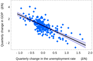
The US «changes in unemployment – GDP growth» regression with the 95% confidence bands.
The confidence intervals for α and β give us the general idea where these regression coefficients are most likely to be. For example, in the Okun’s law regression shown here the point estimates are

The 95% confidence intervals for these estimates are
![{displaystyle alpha in left[,0.76,0.96right],qquad beta in left[-2.06,-1.58,right].}](https://wikimedia.org/api/rest_v1/media/math/render/svg/aca739a7d1ecc8fdddffbdea549b9acba00b464d)
In order to represent this information graphically, in the form of the confidence bands around the regression line, one has to proceed carefully and account for the joint distribution of the estimators. It can be shown[8] that at confidence level (1 − γ) the confidence band has hyperbolic form given by the equation
![{displaystyle (alpha +beta xi )in left[,{widehat {alpha }}+{widehat {beta }}xi pm t_{n-2}^{*}{sqrt {left({frac {1}{n-2}}sum {widehat {varepsilon }}_{i}^{,2}right)cdot left({frac {1}{n}}+{frac {(xi -{bar {x}})^{2}}{sum (x_{i}-{bar {x}})^{2}}}right)}},right].}](https://wikimedia.org/api/rest_v1/media/math/render/svg/7007e876b527e8f59c394898488fd150df4b9f61)
When the model assumed the intercept is fixed and equal to 0 ( ), the standard error of the slope turns into:

With: 
Asymptotic assumption[edit]
The alternative second assumption states that when the number of points in the dataset is «large enough», the law of large numbers and the central limit theorem become applicable, and then the distribution of the estimators is approximately normal. Under this assumption all formulas derived in the previous section remain valid, with the only exception that the quantile t*n−2 of Student’s t distribution is replaced with the quantile q* of the standard normal distribution. Occasionally the fraction 1/n−2 is replaced with 1/n. When n is large such a change does not alter the results appreciably.
Numerical example[edit]
This data set gives average masses for women as a function of their height in a sample of American women of age 30–39. Although the OLS article argues that it would be more appropriate to run a quadratic regression for this data, the simple linear regression model is applied here instead.
-
Height (m), xi 1.47 1.50 1.52 1.55 1.57 1.60 1.63 1.65 1.68 1.70 1.73 1.75 1.78 1.80 1.83 Mass (kg), yi 52.21 53.12 54.48 55.84 57.20 58.57 59.93 61.29 63.11 64.47 66.28 68.10 69.92 72.19 74.46
 |
|
|
 |
 |

|
|---|---|---|---|---|---|
| 1 | 1.47 | 52.21 | 2.1609 | 76.7487 | 2725.8841 |
| 2 | 1.50 | 53.12 | 2.2500 | 79.6800 | 2821.7344 |
| 3 | 1.52 | 54.48 | 2.3104 | 82.8096 | 2968.0704 |
| 4 | 1.55 | 55.84 | 2.4025 | 86.5520 | 3118.1056 |
| 5 | 1.57 | 57.20 | 2.4649 | 89.8040 | 3271.8400 |
| 6 | 1.60 | 58.57 | 2.5600 | 93.7120 | 3430.4449 |
| 7 | 1.63 | 59.93 | 2.6569 | 97.6859 | 3591.6049 |
| 8 | 1.65 | 61.29 | 2.7225 | 101.1285 | 3756.4641 |
| 9 | 1.68 | 63.11 | 2.8224 | 106.0248 | 3982.8721 |
| 10 | 1.70 | 64.47 | 2.8900 | 109.5990 | 4156.3809 |
| 11 | 1.73 | 66.28 | 2.9929 | 114.6644 | 4393.0384 |
| 12 | 1.75 | 68.10 | 3.0625 | 119.1750 | 4637.6100 |
| 13 | 1.78 | 69.92 | 3.1684 | 124.4576 | 4888.8064 |
| 14 | 1.80 | 72.19 | 3.2400 | 129.9420 | 5211.3961 |
| 15 | 1.83 | 74.46 | 3.3489 | 136.2618 | 5544.2916 |
 |
24.76 | 931.17 | 41.0532 | 1548.2453 | 58498.5439 |
There are n = 15 points in this data set. Hand calculations would be started by finding the following five sums:
![{displaystyle {begin{aligned}S_{x}&=sum x_{i},=24.76,qquad S_{y}=sum y_{i},=931.17,\[5pt]S_{xx}&=sum x_{i}^{2}=41.0532,;;,S_{yy}=sum y_{i}^{2}=58498.5439,\[5pt]S_{xy}&=sum x_{i}y_{i}=1548.2453end{aligned}}}](https://wikimedia.org/api/rest_v1/media/math/render/svg/a239d81a6a9897b666146526c8252a18d2603adf)
These quantities would be used to calculate the estimates of the regression coefficients, and their standard errors.
![{displaystyle {begin{aligned}{widehat {beta }}&={frac {nS_{xy}-S_{x}S_{y}}{nS_{xx}-S_{x}^{2}}}=61.272\[8pt]{widehat {alpha }}&={frac {1}{n}}S_{y}-{widehat {beta }}{frac {1}{n}}S_{x}=-39.062\[8pt]s_{varepsilon }^{2}&={frac {1}{n(n-2)}}left[nS_{yy}-S_{y}^{2}-{widehat {beta }}^{2}(nS_{xx}-S_{x}^{2})right]=0.5762\[8pt]s_{widehat {beta }}^{2}&={frac {ns_{varepsilon }^{2}}{nS_{xx}-S_{x}^{2}}}=3.1539\[8pt]s_{widehat {alpha }}^{2}&=s_{widehat {beta }}^{2}{frac {1}{n}}S_{xx}=8.63185end{aligned}}}](https://wikimedia.org/api/rest_v1/media/math/render/svg/1c171ecde06fcbcb38ea0c3e080b7c14efcfdd96)
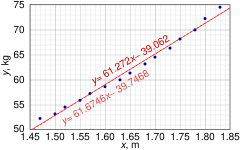
Graph of points and linear least squares lines in the simple linear regression numerical example
The 0.975 quantile of Student’s t-distribution with 13 degrees of freedom is t*13 = 2.1604, and thus the 95% confidence intervals for α and β are
![{displaystyle {begin{aligned}&alpha in [,{widehat {alpha }}mp t_{13}^{*}s_{alpha },]=[,{-45.4}, {-32.7},]\[5pt]&beta in [,{widehat {beta }}mp t_{13}^{*}s_{beta },]=[,57.4, 65.1,]end{aligned}}}](https://wikimedia.org/api/rest_v1/media/math/render/svg/f1e96281c93edfc8cb8e830744328f62081c8010)
The product-moment correlation coefficient might also be calculated:

See also[edit]
- Design matrix#Simple linear regression
- Line fitting
- Linear trend estimation
- Linear segmented regression
- Proofs involving ordinary least squares—derivation of all formulas used in this article in general multidimensional case
References[edit]
- ^ Seltman, Howard J. (2008-09-08). Experimental Design and Analysis (PDF). p. 227.
- ^ «Statistical Sampling and Regression: Simple Linear Regression». Columbia University. Retrieved 2016-10-17.
When one independent variable is used in a regression, it is called a simple regression;(…)
- ^ Lane, David M. Introduction to Statistics (PDF). p. 462.
- ^ Zou KH; Tuncali K; Silverman SG (2003). «Correlation and simple linear regression». Radiology. 227 (3): 617–22. doi:10.1148/radiol.2273011499. ISSN 0033-8419. OCLC 110941167. PMID 12773666.
- ^ Altman, Naomi; Krzywinski, Martin (2015). «Simple linear regression». Nature Methods. 12 (11): 999–1000. doi:10.1038/nmeth.3627. ISSN 1548-7091. OCLC 5912005539. PMID 26824102.
- ^ Kenney, J. F. and Keeping, E. S. (1962) «Linear Regression and Correlation.» Ch. 15 in Mathematics of Statistics, Pt. 1, 3rd ed. Princeton, NJ: Van Nostrand, pp. 252–285
- ^ Valliant, Richard, Jill A. Dever, and Frauke Kreuter. Practical tools for designing and weighting survey samples. New York: Springer, 2013.
- ^ Casella, G. and Berger, R. L. (2002), «Statistical Inference» (2nd Edition), Cengage, ISBN 978-0-534-24312-8, pp. 558–559.
External links[edit]
- Wolfram MathWorld’s explanation of Least Squares Fitting, and how to calculate it
- Mathematics of simple regression (Robert Nau, Duke University)