From Wikipedia, the free encyclopedia

For a value that is sampled with an unbiased normally distributed error, the above depicts the proportion of samples that would fall between 0, 1, 2, and 3 standard deviations above and below the actual value.
The standard error (SE)[1] of a statistic (usually an estimate of a parameter) is the standard deviation of its sampling distribution[2] or an estimate of that standard deviation. If the statistic is the sample mean, it is called the standard error of the mean (SEM).[1]
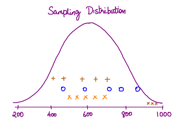
The sampling distribution of a mean is generated by repeated sampling from the same population and recording of the sample means obtained. This forms a distribution of different means, and this distribution has its own mean and variance. Mathematically, the variance of the sampling mean distribution obtained is equal to the variance of the population divided by the sample size. This is because as the sample size increases, sample means cluster more closely around the population mean.
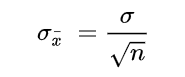
Therefore, the relationship between the standard error of the mean and the standard deviation is such that, for a given sample size, the standard error of the mean equals the standard deviation divided by the square root of the sample size.[1] In other words, the standard error of the mean is a measure of the dispersion of sample means around the population mean.
In regression analysis, the term «standard error» refers either to the square root of the reduced chi-squared statistic or the standard error for a particular regression coefficient (as used in, say, confidence intervals).
Standard error of the sample mean[edit]
Exact value[edit]
Suppose a statistically independent sample of  observations
  is taken from a statistical population with a standard deviation of
  . The mean value calculated from the sample,
  , will have an associated standard error on the mean,
  , given by:[1]
 .
.

Practically this tells us that when trying to estimate the value of a population mean, due to the factor  , reducing the error on the estimate by a factor of two requires acquiring four times as many observations in the sample; reducing it by a factor of ten requires a hundred times as many observations.
Estimate[edit]
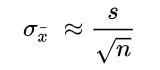
The standard deviation of the population being sampled is seldom known. Therefore, the standard error of the mean is usually estimated by replacing with the sample standard deviation  instead:
- .

As this is only an estimator for the true «standard error», it is common to see other notations here such as:
- or alternately .


A common source of confusion occurs when failing to distinguish clearly between:
Accuracy of the estimator[edit]
When the sample size is small, using the standard deviation of the sample instead of the true standard deviation of the population will tend to systematically underestimate the population standard deviation, and therefore also the standard error. With n = 2, the underestimate is about 25%, but for n = 6, the underestimate is only 5%. Gurland and Tripathi (1971) provide a correction and equation for this effect.[3] Sokal and Rohlf (1981) give an equation of the correction factor for small samples of n < 20.[4] See unbiased estimation of standard deviation for further discussion.
Derivation[edit]
The standard error on the mean may be derived from the variance of a sum of independent random variables,[5] given the definition of variance and some simple properties thereof. If are independent samples from a population with mean and standard deviation , then we can define the total

which due to the Bienaymé formula, will have variance

where we’ve approximated the standard deviations, i.e., the uncertainties, of the measurements themselves with the best value for the standard deviation of the population. The mean of these measurements is simply given by
- .

The variance of the mean is then

The standard error is, by definition, the standard deviation of which is simply the square root of the variance:
- .

For correlated random variables the sample variance needs to be computed according to the Markov chain central limit theorem.
Independent and identically distributed random variables with random sample size[edit]
There are cases when a sample is taken without knowing, in advance, how many observations will be acceptable according to some criterion. In such cases, the sample size  is a random variable whose variation adds to the variation of
  such that,
- [6]

If has a Poisson distribution, then  with estimator
  . Hence the estimator of
  becomes
  , leading the following formula for standard error:

(since the standard deviation is the square root of the variance)
Student approximation when σ value is unknown[edit]
In many practical applications, the true value of σ is unknown. As a result, we need to use a distribution that takes into account that spread of possible σ’s.
When the true underlying distribution is known to be Gaussian, although with unknown σ, then the resulting estimated distribution follows the Student t-distribution. The standard error is the standard deviation of the Student t-distribution. T-distributions are slightly different from Gaussian, and vary depending on the size of the sample. Small samples are somewhat more likely to underestimate the population standard deviation and have a mean that differs from the true population mean, and the Student t-distribution accounts for the probability of these events with somewhat heavier tails compared to a Gaussian. To estimate the standard error of a Student t-distribution it is sufficient to use the sample standard deviation «s» instead of σ, and we could use this value to calculate confidence intervals.
Note: The Student’s probability distribution is approximated well by the Gaussian distribution when the sample size is over 100. For such samples one can use the latter distribution, which is much simpler.
Assumptions and usage[edit]
An example of how  is used is to make confidence intervals of the unknown population mean. If the sampling distribution is normally distributed, the sample mean, the standard error, and the quantiles of the normal distribution can be used to calculate confidence intervals for the true population mean. The following expressions can be used to calculate the upper and lower 95% confidence limits, where is equal to the sample mean, is equal to the standard error for the sample mean, and 1.96 is the approximate value of the 97.5 percentile point of the normal distribution:
- Upper 95% limit and
- Lower 95% limit


In particular, the standard error of a sample statistic (such as sample mean) is the actual or estimated standard deviation of the sample mean in the process by which it was generated. In other words, it is the actual or estimated standard deviation of the sampling distribution of the sample statistic. The notation for standard error can be any one of SE, SEM (for standard error of measurement or mean), or SE.
Standard errors provide simple measures of uncertainty in a value and are often used because:
- in many cases, if the standard error of several individual quantities is known then the standard error of some function of the quantities can be easily calculated;
- when the probability distribution of the value is known, it can be used to calculate an exact confidence interval;
- when the probability distribution is unknown, Chebyshev’s or the Vysochanskiï–Petunin inequalities can be used to calculate a conservative confidence interval; and
- as the sample size tends to infinity the central limit theorem guarantees that the sampling distribution of the mean is asymptotically normal.
Standard error of mean versus standard deviation[edit]
In scientific and technical literature, experimental data are often summarized either using the mean and standard deviation of the sample data or the mean with the standard error. This often leads to confusion about their interchangeability. However, the mean and standard deviation are descriptive statistics, whereas the standard error of the mean is descriptive of the random sampling process. The standard deviation of the sample data is a description of the variation in measurements, while the standard error of the mean is a probabilistic statement about how the sample size will provide a better bound on estimates of the population mean, in light of the central limit theorem.[7]
Put simply, the standard error of the sample mean is an estimate of how far the sample mean is likely to be from the population mean, whereas the standard deviation of the sample is the degree to which individuals within the sample differ from the sample mean.[8] If the population standard deviation is finite, the standard error of the mean of the sample will tend to zero with increasing sample size, because the estimate of the population mean will improve, while the standard deviation of the sample will tend to approximate the population standard deviation as the sample size increases.
Extensions[edit]
Finite population correction (FPC)[edit]
The formula given above for the standard error assumes that the population is infinite. Nonetheless, it is often used for finite populations when people are interested in measuring the process that created the existing finite population (this is called an analytic study). Though the above formula is not exactly correct when the population is finite, the difference between the finite- and infinite-population versions will be small when sampling fraction is small (e.g. a small proportion of a finite population is studied). In this case people often do not correct for the finite population, essentially treating it as an «approximately infinite» population.
If one is interested in measuring an existing finite population that will not change over time, then it is necessary to adjust for the population size (called an enumerative study). When the sampling fraction (often termed f) is large (approximately at 5% or more) in an enumerative study, the estimate of the standard error must be corrected by multiplying by a »finite population correction» (a.k.a.: FPC):[9]
[10]

which, for large N:

to account for the added precision gained by sampling close to a larger percentage of the population. The effect of the FPC is that the error becomes zero when the sample size n is equal to the population size N.
This happens in survey methodology when sampling without replacement. If sampling with replacement, then FPC does not come into play.
Correction for correlation in the sample[edit]

Expected error in the mean of A for a sample of n data points with sample bias coefficient ρ. The unbiased standard error plots as the ρ = 0 diagonal line with log-log slope −½.
If values of the measured quantity A are not statistically independent but have been obtained from known locations in parameter space x, an unbiased estimate of the true standard error of the mean (actually a correction on the standard deviation part) may be obtained by multiplying the calculated standard error of the sample by the factor f:

where the sample bias coefficient ρ is the widely used Prais–Winsten estimate of the autocorrelation-coefficient (a quantity between −1 and +1) for all sample point pairs. This approximate formula is for moderate to large sample sizes; the reference gives the exact formulas for any sample size, and can be applied to heavily autocorrelated time series like Wall Street stock quotes. Moreover, this formula works for positive and negative ρ alike.[11] See also unbiased estimation of standard deviation for more discussion.
See also[edit]
- Illustration of the central limit theorem
- Margin of error
- Probable error
- Standard error of the weighted mean
- Sample mean and sample covariance
- Standard error of the median
- Variance
References[edit]
- ^ a b c d Altman, Douglas G; Bland, J Martin (2005-10-15). «Standard deviations and standard errors». BMJ: British Medical Journal. 331 (7521): 903. doi:10.1136/bmj.331.7521.903. ISSN 0959-8138. PMC 1255808. PMID 16223828.
- ^ Everitt, B. S. (2003). The Cambridge Dictionary of Statistics. CUP. ISBN 978-0-521-81099-9.
- ^ Gurland, J; Tripathi RC (1971). «A simple approximation for unbiased estimation of the standard deviation». American Statistician. 25 (4): 30–32. doi:10.2307/2682923. JSTOR 2682923.
- ^ Sokal; Rohlf (1981). Biometry: Principles and Practice of Statistics in Biological Research (2nd ed.). p. 53. ISBN 978-0-7167-1254-1.
- ^ Hutchinson, T. P. (1993). Essentials of Statistical Methods, in 41 pages. Adelaide: Rumsby. ISBN 978-0-646-12621-0.
- ^ Cornell, J R, and Benjamin, C A, Probability, Statistics, and Decisions for Civil Engineers, McGraw-Hill, NY, 1970, ISBN 0486796094, pp. 178–9.
- ^ Barde, M. (2012). «What to use to express the variability of data: Standard deviation or standard error of mean?». Perspect. Clin. Res. 3 (3): 113–116. doi:10.4103/2229-3485.100662. PMC 3487226. PMID 23125963.
- ^ Wassertheil-Smoller, Sylvia (1995). Biostatistics and Epidemiology : A Primer for Health Professionals (Second ed.). New York: Springer. pp. 40–43. ISBN 0-387-94388-9.
- ^ Isserlis, L. (1918). «On the value of a mean as calculated from a sample». Journal of the Royal Statistical Society. 81 (1): 75–81. doi:10.2307/2340569. JSTOR 2340569. (Equation 1)
- ^ Bondy, Warren; Zlot, William (1976). «The Standard Error of the Mean and the Difference Between Means for Finite Populations». The American Statistician. 30 (2): 96–97. doi:10.1080/00031305.1976.10479149. JSTOR 2683803. (Equation 2)
- ^ Bence, James R. (1995). «Analysis of Short Time Series: Correcting for Autocorrelation». Ecology. 76 (2): 628–639. doi:10.2307/1941218. JSTOR 1941218.
Standard error of the mean measures how spread out the means of the sample can be from the actual population mean. Standard error allows you to build a relationship between a sample statistic (computed from a smaller sample of the population) and the population’s actual parameter.
 Standard Error – A practical guide with examples. Photo by Sergio.
What is Standard Error?
The sample error serves as a means to understand the actual population parameter (like population mean) without actually estimating it.
Consider the following scenario:
A researcher ‘X’ is collecting data from a large population of voters. For practical reasons he can’t reach out to each and every voter. So, only a small randomized sample (of voters) is selected for data collection.
Once the data for the sample is collected, you calculate the mean (or any statistic) of that sample. But then, this mean you just computed is only the sample mean. It cannot be considered the entire population’s mean. You can however expect it to be somewhere close to population’s mean.
So how can you know the actual population mean?
While its not possible to compute the exactly value, you can use standard error to estimate how far the sample mean may spread from the actual population mean.
To be more precise,
The Standard Error of the Mean describes how far a sample mean may vary from the population mean.
In this post, you will understand clearly:
- What Standard Error Tells Us?
- What is the Sample Error Formula?
- How to calculate Standard Error?
- How to use standard error to compute confidence interval?
- Example Problem and solution
How to understand Standard Error?
Let’s first clearly understand the intuition behind and the need for standard error.
Now, let’s suppose you are working in agriculture domain and you want to know the annual yield of a particular variety of coconut trees. While the entire population of coconut trees has a certain mean (and standard deviation) of annual yield, it is not practical to take measurements of each and every tree out there.
So, what do you do?
To estimate this you collect samples of coconut yield (number of nuts per tree per year) from different trees. And to keep your findings unbiased, you collect samples across different places.
MLPlus Industry Data Scientist Program
Do you want to learn Data Science from experienced Data Scientists?
Build your data science career with a globally recognised, industry-approved qualification. Solve projects with real company data and become a certified Data Scientist in less than 12 months.
.
![]()
Get Free Complete Python Course
Build your data science career with a globally recognised, industry-approved qualification. Get the mindset, the confidence and the skills that make Data Scientist so valuable.
Let’s say, you collected data from approx ~5 trees per sample from different places and the numbers are shown below.
# Annual yield of coconut
sample1 = [400, 420, 470, 510, 590]

sample2 = [430, 500, 570, 620, 710, 800, 900]

sample3 = [360, 410, 490, 550, 640]
In above data, the variables sample1, sample2 and sample3 contain the samples of annual yield values collected, where each number represents the yield of one individual tree.
Observe that the yield varies not just across the trees, but also across the different samples.
Although we compute means of the samples, we are actually not interested in the means of the sample, but the overall mean annual yield of coconut of this variety.
Now, you may ask: ‘Why can’t we just put the values from all these samples in one bucket and simply compute the mean and standard deviation and consider that as the population’s parameter?‘
Well, the problem is, if you do that practically what happens is, as you receive few more samples, the real population’s parameter begins to come out which is likely to be (slightly) different from the parameter you computed earlier.
Below is a code demo.
from statistics import mean, stdev

# Overall mean from the first two samples
sample1 = [400, 420, 470, 510, 590]
sample2 = [430, 500, 570, 620, 710, 800, 900]
print("Mean of first two samples: ", mean(sample1 + sample2))

# Overall mean after introducing 3rd sample
sample3 = [360, 410, 490, 550, 640]
print("Mean after including 3rd sample: ", mean(sample1 + sample2 + sample3))
Output:
Mean of first two samples:  576.6666666666666
Mean after including 3rd sample:  551.1764705882352
As you add more and more samples, the computed parameters keep changing.
So how to tackle this?
If you notice, each sample has its own mean that varies between a particular range. This mean (of the sample) has its own standard deviation. This measure of standard deviation of the mean is called the standard error of the mean.
Its important to note, it is different from the standard deviation of the data. The difference is, while standard deviation tells you how the overall data is distributed around the mean, the standard error tells you how the mean itself is distributed.
This way, it can be used to generalize the sample mean so it can be used as an estimate of the whole population.
In fact, standard error can be generalized to any statistic like standard deviation, median etc. For example, if you compute the standard deviation of the standard deviations (of the samples), it is called, standard error of the standard deviation. Feels like a tongue twister. But most commonly, when someone mention ‘Standard error’ it typically refers to the ‘Standard error of of the mean’.
What is the Formula?
To calculate standard error, you simply divide the standard deviation of a given sample by the square root of the total number of items in the sample.
$$SE_{bar{x}} = frac{sigma}{sqrt{n}}$$
where, $SE_{bar{x}}$ is the standard error of the mean, $sigma$ is the standard deviation of the sample and n is the number of items in sample.
Do not confuse this with standard deviation. Because standard error of the sample statistic (like mean) is typically much smaller than the population standard deviation.
Notice few things here:
- The Standard error depends on the number of items in the sample. As you increase the number of items in the sample, lower will be the standard error and more certain you will be about the estimates.
- It uses statistics (standard deviation and number of items) computed from the sample itself, and not of the population. That is, you don’t need to know the population parameters beforehand to compute standard error. This makes it pretty convenient.
- Standard error can also be used as an estimate of how representative a given sample is of a population. The smaller the value, more representative is the sample of the whole population.
Below is a computation for the standard error of the mean:
# Compute Standard Error
sample1 = [400, 420, 470, 510, 590]
se = stdev(sample1)/len(sample1)
print('Standard Error: ', round(se, 2))
Standard Error: 15.19
How to calculate standard error?
Problem Statement
A school aptitude test for 15 year old students studying in a particular territory’s curriculum, is designed to have a mean score of 80 units and a standard deviation of 10 units. A sample of 15 answer papers has a mean score of 85. Can we assume that these 15 scores come from the designated population?
Solution
Our task is to determine if this sample comes from the above mentioned population.
How to solve this?
We approach this problem by computing the standard error of the sample means and use it to compute the confidence interval between which the sample means are expected to fall.
If the given sample mean falls inside this interval, then its safe to assume that the sample comes from the given population.
Time to get into the math.
Using standard error to compute confidence interval
Standard error is often used to compute confidence intervals
We know, n = 15, x_bar = 85, σ = 10
$$SE_bar{x} = frac{sigma}{sqrt{n}} = frac{10}{sqrt{15}} = 2.581$$
From a property of normal distribution, we can say with 95% confidence level that the sample means are expected to lie within a confidence interval of plus or minus two standard errors of the sample statistic from the population parameter.
But where did ‘normal distribution’ come from? You may wonder how we can directly assume a normal distribution is followed in this case. Or rather shouldn’t we test if the sample follows a normal distribution first before computing the confidence intervals.
Well, that’s NOT required. Because, the Central Limit Theorem tells us that even if a population is not normally distributed, a collection of sample means from that population will infact follow a normal distribution. So, its a valid assumption.
Back to the problem, let’s compute the confidence intervals for 95% Confidence Level.
- Lower Limit :
80 - (2*2.581)= 74.838 - Upper Limit :
80 + (2*2.581)= 85.162
So, 95% of our 15 item sample means are expected to fall between 74.838 and 85.162.
Since the sample mean of 85.0 lies within the computed range, there is no reason to believe that the sample does not belong to the population.
Conclusion
Standard error is a commonly used term that we sometimes ignore to fully understand its significance. I hope the concept is clear and you can now relate how you can use standard error in appropriate situations.
Next topic: Confidence Interval
COMPARING TWO INDEPENDENT GROUPS
Rand R. Wilcox, in Applying Contemporary Statistical Techniques, 2003
8.8.2 Bootstrap-t Methods
Bootstrap-t methods for comparing trimmed means are preferable to the percentile bootstrap when the amount of trimming is close to zero. An educated guess is that the bootstrap-t is preferable if the amount of trimming is less than or equal to 10%, but it is stressed that this issue is in need of more research. The only certainty is that with no trimming, all indications are that the bootstrap-t outperforms the percentile bootstrap.
Bootstrap-t methods for comparing trimmed means are performed as follows:
- 1.
-
Compute the sample trimmed means, X¯t1 and X¯t2 and Yuen’s estimate of the squared standard errors, d1 and d2, given by Equation(8.18).
- 2.
-
For each group, generate a bootstrap sample and compute the trimmed means, which we label X¯t1* and X¯t2*. Also, compute Yuen’s estimate of the squared standard error, again using Equation (8.18), which we label d1* and d2*.
- 3.
-
Compute
Ty*=(X¯t1* − X¯t2*)−(X¯t1 − X¯t2)d1*+d2*.
- 4.
-
Repeat steps 2 and 3 B times, yielding Ty1*,…,TyB*. In terms of probability coverage, B = 599 appears to suffice in most situations when α = .05.
- 5.
-
Put the Ty1*,…,TyB* values in ascending order, yielding Ty1*≤…≤TyB*. The Tyb* values (b = 1, …, B) provide an estimate of the distribution of
(X¯t1 − X¯t2)−(μt1−μt2)d1+d2.
- 6.
-
Set ℓ = αB/2 and u = B − ℓ, where ℓ is rounded to the nearest integer.
The equal-tailed 1 − α confidence interval for the difference between the population trimmed means (μt1−μt2) is
(8.26)(X¯t1 − X¯t2−Ty(u)*d1+d2,X¯t1−X¯t2−Ty(ℓ+1)*d1+d2).
To get a symmetric two-sided confidence interval, replace step 3 with
Ty*=|(X¯t1* − X¯t2*)−(X¯t1* − X¯t2*)|d1*+d2*,
set a = (1 − α)B, rounding to the nearest integer, in which case a 1 − α confidence interval for μt1 − μt2 is
(8.27)(X¯t1 − X¯t2)+_Ty(a)*d1+d2.
Hypothesis Testing. As usual, reject the hypothesis of equal population trimmed means (H0: μt1 = μt2) if the 1 − α confidence interval for the difference between the trimmed means does not contain zero. Alternatively, compute Yuen’s test statistic
Ty=X¯t1 − X¯t2d1+d2,
and reject if
Ty<_Ty(ℓ+1)*
or if
Ty>_Ty(u)*.
When using the symmetric, two-sided confidence interval method, reject if|Ty|>_Ty(a)*.
Read full chapter
URL:
https://www.sciencedirect.com/science/article/pii/B9780127515410500298
Multivariate Normal Distribution
J. Tacq, in International Encyclopedia of Education (Third Edition), 2010
Central Limit Theorem
We recall from the article on univariate normal distribution, which was defined by two parameters, mean and variance, that the central limit theorem was very important. This theorem tells us that the sampling distribution of the sample mean, X¯, for a large sample size, is nearly normal, whatever the form of the underlying population distribution (with mean equal to μ, which is the mean of the population, and squared standard error equal to (1/n) (σ2), which is the variance of the population divided by n). It turns out that this theorem can be generalized for the multivariate case: as the sample size is increased, the sampling distribution of the centroid (vector of means) will be multivariate normal, irrespective of the form of the parent population (with centroid equal to μ, which is the centroid of the population, and covariance matrix equal to (1/n) Σ, which is the population covariance matrix divided by n). As we already mentioned, this central limit is the main cause of the immense popularity of the normal distribution and its multivariate counterpart.
Read full chapter
URL:
https://www.sciencedirect.com/science/article/pii/B9780080448947013518
One-Way and Higher Designs for Independent Groups
Rand Wilcox, in Introduction to Robust Estimation and Hypothesis Testing (Third Edition), 2012
7.4.1 An Extension of Yuen’s Method to Trimmed Means
A relatively simple strategy for performing multiple comparisons and tests about linear contrasts, when comparing trimmed means, is to use an extension of Yuen’s method for two groups in conjunction with a simple generalization of Dunnett’s (1980) heteroscedastic T3 procedure for means.
Letting μt1,…, μt j be the trimmed means corresponding to J independent groups, a linear contrast is
Ψ=∑j=1Jcjμtj,
where c1, …, cJ are specified constants satisfying ∑cj=0. As a simple illustration, if c1 = 1, c2 = −1, and c3 = ⋯ = cJ = 0, Ψ = μt1 − μt2, the difference between the first two trimmed means. Typically, C linear contrasts are of interest, a common goal being to compare all pairs of means. Linear contrasts also play an important role when dealing with two-way and higher designs.
Consider testing
(7.7)H0:Ψ=0.
An extension of the Yuen–Welch method accomplishes this goal. The estimate of Ψ is
Ψ^=∑j=1JcjX¯tj.
An estimate of the squared standard error of Ψ^ is
A=∑dj,
where
dj=cj2(nj−1)swj2hj(hj−1),
hj is the effective sample size of the jth group, and swj2 is the Winsorized variance. In other words, estimate the squared standard error of X¯t as is done in Yuen’s method, in which case an estimate of the squared standard error of Ψ^ is given by A. Let
D=∑dj2hj−1,
set
ν^=A2D,
and let t be the 1 − α/2 quantile of Student’s t-distribution with ν^ degrees of freedom. Then an approximate 1 − α confidence interval for Ψ is
Ψ^±tA.
Let Ψ1,…, ΨC be C linear contrasts of interest, where
Ψk=∑j=1Jcjkμtj,
and let ν^k be the estimated degrees of freedom associated with the kth linear contrast, which is computed as described in the previous paragraph. As previously noted, a common goal is to compute a confidence interval for each Ψk such that the simultaneous probability coverage is 1 − α. A related goal is to test H0 : Ψk = 0, k = 1, …, C, such that the familywise error rate (FWE), meaning the probability of at least one type I error among all C tests to be performed, is α, and the practical problem is finding a method that adjusts the critical value to achieve this goal. One strategy is to compute confidence intervals having the form
Ψ^k±tkAk,
where Ak is the estimated squared standard error of Ψ^k, computed as described when testing Eq. (7.7), and tk is the 1 − α percentage point of the C-variate Studentized maximum modulus distribution with estimated degrees of freedom ν^k. In terms of testing H0 : Ψk = 0, k = 1,…, C, reject H0 : Ψk = 0 if |Tk|>tk, where
Tk=Ψ^kAk.
(The R software written for this book determines tk when α = 0.05 or 0.01, and C ≤ 28 using values computed and reported in Wilcox, 1986. For other values of α or C > 28, the function determines tk via simulations with 10,000 replications. Bechhofer & Dunnett, 1982, report values up to C = 32.) When there is no trimming, the method just described reduces to Dunnett’s (1980) T3 procedure for means when all pairwise comparisons are performed.
Read full chapter
URL:
https://www.sciencedirect.com/science/article/pii/B978012386983800007X
MULTIPLE COMPARISONS
Rand R. Wilcox, in Applying Contemporary Statistical Techniques, 2003
Welch–Šidák Method
The first contains Dunnett’s T3 method as a special case and is called the Welch-Šidák method. (The computations are performed by the S-PLUS function lincon described in Section 12.6.1.) Again let L represent the total number of groups being compared, let Ψ be any linear contrast of interest, and let C represent the total number of contrasts to be tested. An expression for the squared standard error of Ψ^ is
σΨ^2=∑cℓ2σℓ2nℓ,
where σℓ2 and nℓ are the variance and sample size of the ℓth group, respectively. An estimate of this quantity is obtained simply by replacing σℓ2 with sℓ2, the sample variance associated with the ℓth group. That is, estimate σΨ^2 with
σ^Ψ^2=∑cℓ2sℓ2nℓ.
Let
qℓ=cℓ2sℓ2nℓ.
The degrees of freedom are estimated to be
v^=(∑qℓ)2∑qℓ2nℓ−1.
The test statistic is
T=Ψ^σ^Ψ^.
The critical value, c, is a function of v^ and C (the total number of hypotheses you plan to perform) and is read from Table 10 in Appendix B. Reject if |T| ≥ c, and a confidence interval for Ψ is
(12.9)Ψ^±cσ^Ψ^.
Read full chapter
URL:
https://www.sciencedirect.com/science/article/pii/B978012751541050033X
Comparing Two Groups
Rand Wilcox, in Introduction to Robust Estimation and Hypothesis Testing (Third Edition), 2012
Method M1
The first method is based on a straightforward generalization of the method in Lin and Stivers (1974), assuming that the goal is to compare the marginal trimmed means, as opposed to the trimmed mean of the difference scores. It is assumed than n pairs of observations are randomly sampled where both values are available, which is denoted by (X1,Y1),…,(Xn,Yn). The corresponding (marginal) γ-trimmed means are denoted by X¯t and Y¯t. For the first marginal distribution, an additional n1 observations are sampled for which the corresponding Y value is not observed. These observations are denoted by Xn+1,…,Xn+n1 and the trimmed mean of these n1 observations is denoted by X˜t. Similarly, n2 observations are sampled for which the corresponding value for the first marginal distribution is not observed and the trimmed mean is denoted by Ỹt. Let hj=[γnj] (j = 1, 2), and let λj=h∕(h+hj), where h = [γn]. Then an estimate of the difference between the marginal trimmed means, Δt = μt1 − μt2, is
μ^tD=λ1X¯tD−λ2Y¯tD+(1−λ1)X˜tD−(1−λ2)ỸtD,
a linear combination of three independent random variables. The squared standard of λ1X¯−λ2Y¯ is
(5.26)σ02=1(1−2γ)2n(λ12σwx2+λ2σwy2−2λ1λ2σwxy),
where σwxy is the population Winsorized covariance between X and Y. The squared standard error of (1−λ1)X˜ is
(5.27)σ12=(1−λ1)2σwx2(1−2γ)2(n+n1)
and the squared standard error of (1−λ2)Ỹ is
(5.28)σ22=(1−λ2)2σwy2(1−2γ)2(n+n2).
So the squared standard error of μ^tD is
τ2=σ02+σ12+σ22.
For convenience, let N1 = n + n1 and g1 = [γN1]. The Winsorized values corresponding to X1,…,XN1 are
Wxi={X(g1+1) if Xi≤X(g1+1)Xi if X(g1+1)<Xi<X(N1−g1)X(N1−g1) if Xi≥X(N1−g1).
The (sample) Winsorized mean is
W¯x=1N1∑i=1N1Wxi,
an estimate of the Winsorized variance, σwx2, is
swx2=1N1−1∑(Wxi−W¯x)2,
and an estimate of σwy2 is obtained in a similar fashion. The Winsorized covariance between X and Y is estimated with
swxy=1n−1∑i−1n(Wxi−W˜x)(Wyi−W˜y),
where
X˜w=1n∑i=1nWxi
and Ỹw is defined in a similar manner.
The sample Winsorized variances yield estimates of σ02, σ12 and σ22, say σ^02, σ^12 and σ^22, in which case an estimate of the squared standard error of μ^tD is
τ^2=σ^02+σ^12+σ^22.
So a reasonable test statistic for testing the hypothesis of equal (marginal) trimmed means is
(5.29)T=μ^tDτ^.
There remains the problem of approximating the null distribution of T and here a basic bootstrap-t method is used. To make sure the details are clear, the method begins by randomly sampling with replacement N = n + n1 + n2 pairs of observations from (X1,Y2),…,(XN,YN) yielding (X1∗,Y2∗),…,(XN∗,YN∗). Based on this bootstrap sample, compute the absolute value of the test statistic as just described and label the result T*. Repeat this process B times and put the resulting T* values in ascending order yielding T(1)∗≤⋯≤T(B)∗. Then an approximate 1 − α confidence interval for Δt is
Δ^t±T(c)∗τ^
where c=(1−α)B rounded to the nearest integer.
Read full chapter
URL:
https://www.sciencedirect.com/science/article/pii/B9780123869838000056
Comparing Two Groups
Rand R. Wilcox, in Introduction to Robust Estimation and Hypothesis Testing (Fifth Edition), 2022
Method M1
The first method is based on a straightforward generalization of the method in Lin and Stivers (1974), assuming that the goal is to compare the marginal trimmed means, as opposed to the trimmed mean of the difference scores. It is assumed than n pairs of observations are randomly sampled, where both values are available, which is denoted by (X1,Y1),…,(Xn,Yn). The corresponding (marginal) γ-trimmed means are denoted by X¯t and Y¯t. For the first marginal distribution, additional n1 observations are sampled for which the corresponding Y value is not observed. These observations are denoted by Xn+1,…,Xn+n1, and the trimmed mean of these n1 observations is denoted by X˜t. Similarly, n2 observations are sampled for which the corresponding value for the first marginal distribution is not observed and the trimmed mean is denoted by Y˜t. Let hj=[γnj] (j=1, 2), and let λj=h/(h+hj), where h=[γn]. Then an estimate of the difference between the marginal trimmed means, μtD=μt1−μt2, is
μˆtD=λ1X¯t−λ2Y¯t+(1−λ1)X˜t−(1−λ2)Y˜t,
a linear combination of three independent random variables. The squared standard of λ1X¯−λ2Y¯ is
(5.38)σ02=1(1−2γ)2n(λ12σwx2+λ2σwy2−2λ1λ2σwxy),
where σwxy is the population Winsorized covariance between X and Y. The squared standard error of (1−λ1)X˜ is
(5.39)σ12=(1−λ1)2σwx2(1−2γ)2(n+n1)
and the squared standard error of (1−λ2)Y˜ is
(5.40)σ22=(1−λ2)2σwy2(1−2γ)2(n+n2).
So, the squared standard error of μˆtD is
τ2=σ02+σ12+σ22.
For convenience, let N1=n+n1 and g1=[γN1]. The Winsorized values corresponding to X1,…,XN1 are
Wxi={X(g1+1),if Xi≤X(g1+1),Xi,if X(g1+1)<Xi<X(N1−g1),X(N1−g1),if Xi≥X(N1−g1).
The (sample) Winsorized mean is
W¯x=1N1∑i=1N1Wxi,
an estimate of the Winsorized variance, σwx2, is
swx2=1N1−1∑(Wxi−W¯x)2,
and an estimate of σwy2 is obtained in a similar fashion. The Winsorized covariance between X and Y is estimated with
swxy=1n−1∑i−1n(Wxi−W˜x)(Wyi−W˜y),
where
W˜x=1n∑i=1nWxi
and W˜y is defined in a similar manner.
The sample Winsorized variances yield estimates of σ02, σ12, and σ22, say σˆ02, σˆ12, and σˆ22, in which case, an estimate of the squared standard error of μˆtD is
τˆ2=σˆ02+σˆ12+σˆ22.
So, a reasonable test statistic for testing the hypothesis of equal (marginal) trimmed means is
(5.41)T=μˆtDτˆ.
There remains the problem of approximating the null distribution of T, and here, a basic bootstrap-t method is used. To make sure the details are clear, the method begins by randomly sampling with replacement N=n+n1+n2 pairs of observations from (X1,Y2),…,(XN,YN), yielding (X1⁎,Y2⁎),…,(XN⁎,YN⁎). Based on this bootstrap sample, compute the absolute value of the test statistic as just described, and label the result T⁎. Repeat this process B times, and put the resulting T⁎ values in ascending order, yielding T(1)⁎≤⋯≤T(B)⁎. Then an approximate 1−α confidence interval for Δt is
Δˆt±T(c)⁎τˆ,
where c=(1−α)B rounded to the nearest integer.
Read full chapter
URL:
https://www.sciencedirect.com/science/article/pii/B9780128200988000117
ANCOVA
Rand R. Wilcox, in Introduction to Robust Estimation and Hypothesis Testing (Fifth Edition), 2022
12.5.1 Methods Based on a Linear Model
Let ydi=yi1−yi2 (i=1,…,n) and assume that the typical value of yd, given x, is given by m(x)=β0+β1x. (Of course, x could be a difference score as well.) Then the method in Section 11.1.12 and the R functions in Section 11.1.13 can be used to make inferences about m(yd). In particular, H0: m(x)=0 can be tested for a range of x values via the R function in Section 11.1.13.
It is briefly noted that in the context of a pretest-posttest study, there are concerns about using pretest scores as the covariate. For a discussion of this issue, see for example Erikkson and Häggström (2014).
As for testing H0: m1(x)=m2(x) when yi1 and yi2 are dependent, the ANCOVA methods described in Section 12.1 are readily modified to handle this situation. Let mˆj(x) be some estimate of mj(x) based on (xij,yij) (j=1, 2) and let δ=m1(x)−m2(x). The first step is to estimate the squared standard error of δˆ=mˆ1(x)−mˆ2(x) in a manner that takes into account that the corresponding estimates are dependent.
Let (xi1⁎,yi1⁎,xi2⁎,yi2⁎), i=1,…,n, be a bootstrap sample. Based on this bootstrap sample, and for a single value of the covariate, x, let mˆj⁎(x)=b0⁎+b1⁎x, where b0⁎ and b1⁎ are estimates of the intercept and slope, respectively, based on (xij⁎,yij⁎), j=1, 2. Let
D⁎=mˆ1⁎(x)−mˆ2⁎(x).
Repeat this process B times, yielding Db⁎ (b=1,…,B). Then an estimate of the squared standard error of δˆ is
τˆ2=1B−1∑(Db⁎−D¯⁎)2,
where D¯⁎=∑Db/B. An appropriate test statistic for testing H0: δ=θ0, where θ0 is some specified constant, is
W=D−θ0τˆ.
When using the Theil–Sen estimator, simulations indicate that W has, approximately, a standard normal distribution. When using least squares regression, assume W has, approximately, a Student’s t distribution with n−1 degrees of freedom (Wilcox and Clark, 2014).
One strategy for choosing the covariate values when testing H0: m1(x)=m2(x) is to proceed along the lines in Section 12.2.1 using the data associated with the first covariate. This approach is assumed unless stated otherwise. As for controlling the probability of one or more Type I errors when testing K hypotheses based on K values of the covariate, using the Studentized maximum modulus distribution with infinite degrees of freedom appears to perform well when K=5. (As for least squares regression, again the degrees of freedom are taken to be n−1.)
Read full chapter
URL:
https://www.sciencedirect.com/science/article/pii/B978012820098800018X
LEAST SQUARES REGRESSION AND PEARSON’S CORRELATION
Rand R. Wilcox, in Applying Contemporary Statistical Techniques, 2003
6.3.3 Restricting the Range of Y
The derivation of the inferential methods in Section 6.3.1 treats the X values as constants and the Y values as random variables. That is, the methods are derived by conditioning on the X values, which makes it a fairly simple matter to derive an estimate of the standard error of the least squares estimate of the slope and intercept. For example, we saw that
b1=∑wiYi,
where
wi=Xi−X¯(n−1)sx2
Treating the X values as constants, and using the rules of expected values in Chapter 2, it can be shown that the squared standard error of b1 is given by
(6.11)wi=Xi−X¯(n−1)sx2
as noted in Section 6.3.1. A practical implication is that if we restrict the range of X values, no technical problems arise when trying to estimate the standard error of b1; we simply use Equation (6 .11) on the points that remain (with n reduced to the number of points remaining). But if we restrict the range of Y values by eliminating outliers, the methods in Section 6.3.1 are no longer valid, even under normality and homoscedasticity. We saw in Section 4.9.1 that if we eliminate extreme values and compute the mean using the data that remain, the standard error of this mean should not be estimated with the sample variance based on the data that remain. A similar problem arises here. If we eliminate extreme Y values, the remaining Y values are no longer independent. So if we use least squares to estimate the slope based on the pairs of points not eliminated, estimating the standard error of the slope becomes a nontrivial problem — the dependence among the Y values must be taken into account.
Read full chapter
URL:
https://www.sciencedirect.com/science/article/pii/B9780127515410500274
Estimating Measures of Location and Scale
Rand Wilcox, in Introduction to Robust Estimation and Hypothesis Testing (Fourth Edition), 2017
3.6.6 A Bootstrap Estimate of the Standard Error of μˆm
The standard error can also be estimated using a bootstrap method. The computational details are essentially the same as those described in Section 3.1. Begin by drawing a bootstrap sample, X1⁎,…,Xn⁎ from the observed values X1,…,Xn. That is, randomly sample n observations with replacement from X1,…,Xn. Compute the value of μˆm using the bootstrap sample and label the result μˆm⁎. Repeat this process B times yielding μˆm1⁎,…,μˆmB⁎. Let
μ¯⁎=1B∑b=1Bμˆmb⁎,
in which case the bootstrap estimate of the squared standard error is
(3.33)σˆmboot2=1B−1∑b=1B(μˆmb⁎−μ¯⁎)2.
Using B=25 might suffice, while B=100 appears to be more than adequate in most situations (Efron, 1987).
A negative feature of the bootstrap is that if n is large, execution time can be high, even on a mainframe computer, when working with various software packages designed specifically for doing statistics. The accuracy of the bootstrap method versus the kernel density estimator has not been examined when n is small. Early attempts at comparing the two estimators, via simulations, were complicated by the problem that the kernel density estimator that was used can be undefined because of division by zero. Yet another problem is that the bootstrap method can fail when n is small because a bootstrap sample can yield MAD=0, in which case μˆm⁎ cannot be computed because of division by zero. A few checks were made with n=20 and B=1000 when sampling from a normal or lognormal distribution. Limited results suggest that the bootstrap is more accurate, but a more detailed study is needed to resolve this issue.
Read full chapter
URL:
https://www.sciencedirect.com/science/article/pii/B9780128047330000032
![]()
Download Article
![]()
Download Article
The standard error of estimate is used to determine how well a straight line can describe values of a data set. When you have a collection of data from some measurement, experiment, survey or other source, you can create a line of regression to estimate additional data. With the standard error of estimate, you get a score that describes how good the regression line is.
-
1
Create a five column data table. Any statistical work is generally made easier by having your data in a concise format. A simple table serves this purpose very well. To calculate the standard error of estimate, you will be using five different measurements or calculations. Therefore, creating a five-column table is helpful. Label the five columns as follows:[1]
-
2
Enter the data values for your measured data. After collecting your data, you will have pairs of data values. For these statistical calculations, the independent variable is labeled
and the dependent, or resulting, variable is . Enter these values into the first two columns of your data table.[2]
- The order of the data and the pairing is important for these calculations. You need to be careful to keep your paired data points together in order.
- For the sample calculations shown above, the data pairs are as follows:
- (1,2)
- (2,4)
- (3,5)
- (4,4)
- (5,5)
Advertisement
-
3
Calculate a regression line. Using your data results, you will be able to calculate a regression line. This is also called a line of best fit or the least squares line. The calculation is tedious but can be done by hand. Alternatively, you can use a handheld graphing calculator or some online programs that will quickly calculate a best fit line using your data.[3]
- For this article, it is assumed that you will have the regression line equation available or that it has been predicted by some prior means.
- For the sample data set in the image above, the regression line is .
-
4
Calculate predicted values from the regression line. Using the equation of that line, you can calculate predicted y-values for each x-value in your study, or for other theoretical x-values that you did not measure.[4]


Advertisement
-
1
Calculate the error of each predicted value. In the fourth column of your data table, you will calculate and record the error of each predicted value. Specifically, subtract the predicted value (
) from the actual observed value ().[5]
- For the data in the sample set, these calculations are as follows:
-
2
Calculate the squares of the errors. Take each value in the fourth column and square it by multiplying it by itself. Fill in these results in the final column of your data table.
- For the sample data set, these calculations are as follows:
-
3
Find the sum of the squared errors (SSE). The statistical value known as the sum of squared errors (SSE) is a useful step in finding standard deviation, variance and other measurements. To find the SSE from your data table, add the values in the fifth column of your data table.[6]
- For this sample data set, this calculation is as follows:
- For this sample data set, this calculation is as follows:
-
4
Finalize your calculations. The Standard Error of the Estimate is the square root of the average of the SSE. It is generally represented with the Greek letter
. Therefore, the first calculation is to divide the SSE score by the number of measured data points. Then, find the square root of that result.[7]
- If the measured data represents an entire population, then you will find the average by dividing by N, the number of data points. However, if you are working with a smaller sample set of the population, then substitute N-2 in the denominator.
- For the sample data set in this article, we can assume that it is a sample set and not a population, just because there are only 5 data values. Therefore, calculate the Standard Error of the Estimate as follows:
-
5
Interpret your result. The Standard Error of the Estimate is a statistical figure that tells you how well your measured data relates to a theoretical straight line, the line of regression. A score of 0 would mean a perfect match, that every measured data point fell directly on the line. Widely scattered data will have a much higher score.[8]
- With this small sample set, the standard error score of 0.894 is quite low and represents well organized data results.


Advertisement
Ask a Question
200 characters left
Include your email address to get a message when this question is answered.
Submit
Advertisement
Video
Thanks for submitting a tip for review!
References
About This Article
Article SummaryX
To calculate the standard error of estimate, create a five-column data table. In the first two columns, enter the values for your measured data, and enter the values from the regression line in the third column. In the fourth column, calculate the predicted values from the regression line using the equation from that line. These are the errors. Fill in the fifth column by multiplying each error by itself. Add together all of the values in column 5, then take the square root of that number to get the standard error of estimate. To learn how to organize the data pairs, keep reading!
Did this summary help you?
Thanks to all authors for creating a page that has been read 186,557 times.
Did this article help you?
When we fit a regression model to a dataset, we’re often interested in how well the regression model “fits” the dataset. Two metrics commonly used to measure goodness-of-fit include R-squared (R2) and the standard error of the regression, often denoted S.
This tutorial explains how to interpret the standard error of the regression (S) as well as why it may provide more useful information than R2.
Standard Error vs. R-Squared in Regression
Suppose we have a simple dataset that shows how many hours 12 students studied per day for a month leading up to an important exam along with their exam score:

If we fit a simple linear regression model to this dataset in Excel, we receive the following output:

R-squared is the proportion of the variance in the response variable that can be explained by the predictor variable. In this case, 65.76% of the variance in the exam scores can be explained by the number of hours spent studying.
The standard error of the regression is the average distance that the observed values fall from the regression line. In this case, the observed values fall an average of 4.89 units from the regression line.
If we plot the actual data points along with the regression line, we can see this more clearly:

Notice that some observations fall very close to the regression line, while others are not quite as close. But on average, the observed values fall 4.19 units from the regression line.
The standard error of the regression is particularly useful because it can be used to assess the precision of predictions. Roughly 95% of the observation should fall within +/- two standard error of the regression, which is a quick approximation of a 95% prediction interval.
If we’re interested in making predictions using the regression model, the standard error of the regression can be a more useful metric to know than R-squared because it gives us an idea of how precise our predictions will be in terms of units.
To illustrate why the standard error of the regression can be a more useful metric in assessing the “fit” of a model, consider another example dataset that shows how many hours 12 students studied per day for a month leading up to an important exam along with their exam score:

Notice that this is the exact same dataset as before, except all of the values are cut in half. Thus, the students in this dataset studied for exactly half as long as the students in the previous dataset and received exactly half the exam score.
If we fit a simple linear regression model to this dataset in Excel, we receive the following output:

Notice that the R-squared of 65.76% is the exact same as the previous example.
However, the standard error of the regression is 2.095, which is exactly half as large as the standard error of the regression in the previous example.
If we plot the actual data points along with the regression line, we can see this more clearly:

Notice how the observations are packed much more closely around the regression line. On average, the observed values fall 2.095 units from the regression line.
So, even though both regression models have an R-squared of 65.76%, we know that the second model would provide more precise predictions because it has a lower standard error of the regression.
The Advantages of Using the Standard Error
The standard error of the regression (S) is often more useful to know than the R-squared of the model because it provides us with actual units. If we’re interested in using a regression model to produce predictions, S can tell us very easily if a model is precise enough to use for prediction.
For example, suppose we want to produce a 95% prediction interval in which we can predict exam scores within 6 points of the actual score.
Our first model has an R-squared of 65.76%, but this doesn’t tell us anything about how precise our prediction interval will be. Luckily we also know that the first model has an S of 4.19. This means a 95% prediction interval would be roughly 2*4.19 = +/- 8.38 units wide, which is too wide for our prediction interval.
Our second model also has an R-squared of 65.76%, but again this doesn’t tell us anything about how precise our prediction interval will be. However, we know that the second model has an S of 2.095. This means a 95% prediction interval would be roughly 2*2.095= +/- 4.19 units wide, which is less than 6 and thus sufficiently precise to use for producing prediction intervals.
Further Reading
Introduction to Simple Linear Regression
What is a Good R-squared Value?
A mathematical tool used in statistics to measure variability
What is Standard Error?
Standard error is a mathematical tool used in statistics to measure variability. It enables one to arrive at an estimation of what the standard deviation of a given sample is. It is commonly known by its abbreviated form – SE.

Standard error is used to estimate the efficiency, accuracy, and consistency of a sample. In other words, it measures how precisely a sampling distribution represents a population.
It can be applied in statistics and economics. It is especially useful in the field of econometrics, where researchers use it in performing regression analyses and hypothesis testing. It is also used in inferential statistics, where it forms the basis for the construction of the confidence intervals.
Some commonly used measures in the field of statistics include:
- Standard error of the mean (SEM)
- Standard error of the variance
- Standard error of the median
- Standard error of a regression coefficient
Calculating Standard Error of the Mean (SEM)
The SEM is calculated using the following formula:
Where:
- σ – Population standard deviation
- n – Sample size, i.e., the number of observations in the sample
In a situation where statisticians are ignorant of the population standard deviation, they use the sample standard deviation as the closest replacement. SEM can then be calculated using the following formula. One of the primary assumptions here is that observations in the sample are statistically independent.
Where:
- s – Sample standard deviation
- n – Sample size, i.e., the number of observations in the sample
Importance of Standard Error
When a sample of observations is extracted from a population and the sample mean is calculated, it serves as an estimate of the population mean. Almost certainly, the sample mean will vary from the actual population mean. It will aid the statistician’s research to identify the extent of the variation. It is where the standard error of the mean comes into play.
When several random samples are extracted from a population, the standard error of the mean is essentially the standard deviation of different sample means from the population mean.
However, multiple samples may not always be available to the statistician. Fortunately, the standard error of the mean can be calculated from a single sample itself. It is calculated by dividing the standard deviation of the observations in the sample by the square root of the sample size.
Relationship between SEM and the Sample Size
Intuitively, as the sample size increases, the sample becomes more representative of the population.
For example, consider the marks of 50 students in a class in a mathematics test. Two samples A and B of 10 and 40 observations, respectively, are extracted from the population. It is logical to assert that the average marks in sample B will be closer to the average marks of the whole class than the average marks in sample A.
Thus, the standard error of the mean in sample B will be smaller than that in sample A. The standard error of the mean will approach zero with the increasing number of observations in the sample, as the sample becomes more and more representative of the population, and the sample mean approaches the actual population mean.
It is evident from the mathematical formula of the standard error of the mean that it is inversely proportional to the sample size. It can be verified using the SEM formula that if the sample size increases from 10 to 40 (becomes four times), the standard error will be half as big (reduces by a factor of 2).
Standard Deviation vs. Standard Error of the Mean
Standard deviation and standard error of the mean are both statistical measures of variability. While the standard deviation of a sample depicts the spread of observations within the given sample regardless of the population mean, the standard error of the mean measures the degree of dispersion of sample means around the population mean.
Related Readings
CFI is the official provider of the Business Intelligence & Data Analyst (BIDA)® certification program, designed to transform anyone into a world-class financial analyst.
To keep learning and developing your knowledge of financial analysis, we highly recommend the additional resources below:
- Coefficient of Variation
- Basic Statistics Concepts for Finance
- Regression Analysis
- Arithmetic Mean
- See all data science resources
In statistics, the standard error is the standard deviation of the sample distribution. The sample mean of a data is generally varied from the actual population mean. It is represented as SE. It is used to measure the amount of accuracy by which the given sample represents its population. Statistics is a vast topic in which we learn about data, sample and population, mean, median, mode, dependent and independent variables, standard deviation, variance, etc. Here you will learn the standard error formula along with SE of the mean and estimation.
Table of contents:
- Meaning
- SE Formula
- SE of Mean
- SE of Estimate
- Calculation of SE
- Example
- SE vs SD
- Importance
- FAQs
Standard Error Meaning
The standard error is one of the mathematical tools used in statistics to estimate the variability. It is abbreviated as SE. The standard error of a statistic or an estimate of a parameter is the standard deviation of its sampling distribution. We can define it as an estimate of that standard deviation.
The accuracy of a sample that describes a population is identified through the SE formula. The sample mean which deviates from the given population and that deviation is given as;

Where S is the standard deviation and n is the number of observations.
Standard Error of the Mean (SEM)
The standard error of the mean also called the standard deviation of mean, is represented as the standard deviation of the measure of the sample mean of the population. It is abbreviated as SEM. For example, normally, the estimator of the population mean is the sample mean. But, if we draw another sample from the same population, it may provide a distinct value.
Thus, there would be a population of the sampled means having its distinct variance and mean. It may be defined as the standard deviation of such sample means of all the possible samples taken from the same given population. SEM defines an estimate of standard deviation which has been computed from the sample. It is calculated as the ratio of the standard deviation to the root of sample size, such as:
 .
.
Where ‘s’ is the standard deviation and n is the number of observations.
The standard error of the mean shows us how the mean changes with different tests, estimating the same quantity. Thus if the outcome of random variations is notable, then the standard error of the mean will have a higher value. But, if there is no change observed in the data points after repeated experiments, then the value of the standard error of the mean will be zero.
Standard Error of Estimate (SEE)
The standard error of the estimate is the estimation of the accuracy of any predictions. It is denoted as SEE. The regression line depreciates the sum of squared deviations of prediction. It is also known as the sum of squares error. SEE is the square root of the average squared deviation. The deviation of some estimates from intended values is given by standard error of estimate formula.

Where xi stands for data values, x bar is the mean value and n is the sample size.
Also check:
- Standard Error Formula
- Standard Error Calculator
- Standard Deviation Formula
How to calculate Standard Error
Step 1: Note the number of measurements (n) and determine the sample mean (μ). It is the average of all the measurements.
Step 2: Determine how much each measurement varies from the mean.
Step 3: Square all the deviations determined in step 2 and add altogether: Σ(xi – μ)²
Step 4: Divide the sum from step 3 by one less than the total number of measurements (n-1).
Step 5: Take the square root of the obtained number, which is the standard deviation (σ).
Step 6: Finally, divide the standard deviation obtained by the square root of the number of measurements (n) to get the standard error of your estimate.
Go through the example given below to understand the method of calculating standard error.
Standard Error Example
Calculate the standard error of the given data:
y: 5, 10, 12, 15, 20
Solution: First we have to find the mean of the given data;
Mean = (5+10+12+15+20)/5 = 62/5 = 10.5
Now, the standard deviation can be calculated as;
S = Summation of difference between each value of given data and the mean value/Number of values.
Hence,

After solving the above equation, we get;
S = 5.35
Therefore, SE can be estimated with the formula;
SE = S/√n
SE = 5.35/√5 = 2.39
Standard Error vs Standard Deviation
The below table shows how we can calculate the standard deviation (SD) using population parameters and standard error (SE) using sample parameters.
| Population parameters | Formula for SD | Sample statistic | Formula for SE |
| Mean
(begin{array}{l}bar{x}end{array} ) |
(begin{array}{l}frac{sigma }{sqrt{n}}end{array} ) |
Sample mean
(begin{array}{l}bar{x}end{array} ) |
(begin{array}{l}frac{s}{sqrt{n}}end{array} ) |
| Sample proportion (P) |
(begin{array}{l}sqrt{frac{P(1-P)}{n}}end{array} ) |
Sample proportion (p) |
(begin{array}{l}sqrt{frac{p(1-p)}{n}}end{array} ) |
| Difference between means
(begin{array}{l}bar{x_1}-bar{x_2}end{array} ) |
(begin{array}{l}sqrt{frac{sigma_1^2}{n_1}+frac{sigma_2^2}{n_2}}end{array} ) |
Difference between means
(begin{array}{l}bar{x_1}-bar{x_2}end{array} ) |
(begin{array}{l}sqrt{frac{s_1^2}{n_1}+frac{s_2^2}{n_2}}end{array} ) |
| Difference between proportions P1 – P2 |
(begin{array}{l}sqrt{frac{P_1(1-P_1)}{n_1}+frac{P_2(1-P_2)}{n_2}}end{array} ) |
Difference between proportions p1 – p2 |
(begin{array}{l}sqrt{frac{p_1(1-p_1)}{n_1}+frac{p_2(1-p_2)}{n_2}}end{array} ) |
Importance of Standard Error
Standard errors produce simplistic measures of uncertainty in a value. They are often used because, in many cases, if the standard error of some individual quantities is known, then we can easily calculate the standard error of some function of the quantities. Also, when the probability distribution of the value is known, we can use it to calculate an exact confidence interval. However, the standard error is an essential indicator of how precise an estimate of the sample statistic’s population parameter is.
Frequently Asked Questions – FAQs
How do you calculate standard error?
The standard error is calculated by dividing the standard deviation by the sample size’s square root. It gives the precision of a sample mean by including the sample-to-sample variability of the sample means.
What does the standard error mean?
The standard error of a statistic or an estimate of a parameter is the standard deviation of its sampling distribution.
Is standard error the same as SEM?
The standard error (SE) can be defined more precisely like the standard error of the mean (SEM) and is a property of our estimate of the mean.
What is a good standard error?
SE is an implication of the expected precision of the sample mean as compared with the population mean. The bigger the value of standard error, the more the spread and likelihood that any sample means are not close to the population’s mean. A small standard error is thus a good attribute.
What is a big standard error?
The bigger the standard error, the more the spread means there will be less accurate statistics.