From Wikipedia, the free encyclopedia
In mathematical optimization and decision theory, a loss function or cost function (sometimes also called an error function) [1] is a function that maps an event or values of one or more variables onto a real number intuitively representing some «cost» associated with the event. An optimization problem seeks to minimize a loss function. An objective function is either a loss function or its opposite (in specific domains, variously called a reward function, a profit function, a utility function, a fitness function, etc.), in which case it is to be maximized. The loss function could include terms from several levels of the hierarchy.
In statistics, typically a loss function is used for parameter estimation, and the event in question is some function of the difference between estimated and true values for an instance of data. The concept, as old as Laplace, was reintroduced in statistics by Abraham Wald in the middle of the 20th century.[2] In the context of economics, for example, this is usually economic cost or regret. In classification, it is the penalty for an incorrect classification of an example. In actuarial science, it is used in an insurance context to model benefits paid over premiums, particularly since the works of Harald Cramér in the 1920s.[3] In optimal control, the loss is the penalty for failing to achieve a desired value. In financial risk management, the function is mapped to a monetary loss.
Examples[edit]
Regret[edit]
Leonard J. Savage argued that using non-Bayesian methods such as minimax, the loss function should be based on the idea of regret, i.e., the loss associated with a decision should be the difference between the consequences of the best decision that could have been made had the underlying circumstances been known and the decision that was in fact taken before they were known.
Quadratic loss function[edit]
The use of a quadratic loss function is common, for example when using least squares techniques. It is often more mathematically tractable than other loss functions because of the properties of variances, as well as being symmetric: an error above the target causes the same loss as the same magnitude of error below the target. If the target is t, then a quadratic loss function is

for some constant C; the value of the constant makes no difference to a decision, and can be ignored by setting it equal to 1. This is also known as the squared error loss (SEL). [1]
Many common statistics, including t-tests, regression models, design of experiments, and much else, use least squares methods applied using linear regression theory, which is based on the quadratic loss function.
The quadratic loss function is also used in linear-quadratic optimal control problems. In these problems, even in the absence of uncertainty, it may not be possible to achieve the desired values of all target variables. Often loss is expressed as a quadratic form in the deviations of the variables of interest from their desired values; this approach is tractable because it results in linear first-order conditions. In the context of stochastic control, the expected value of the quadratic form is used.
0-1 loss function[edit]
In statistics and decision theory, a frequently used loss function is the 0-1 loss function

where  is the indicator function.
Meaning if the input is evaluated to true, then the output is 1. Otherwise, if the input is evaluated to false, then the output will be 0.
Constructing loss and objective functions[edit]
In many applications, objective functions, including loss functions as a particular case, are determined by the problem formulation. In other situations, the decision maker’s preference must be elicited and represented by a scalar-valued function (called also utility function) in a form suitable for optimization — the problem that Ragnar Frisch has highlighted in his Nobel Prize lecture.[4]
The existing methods for constructing objective functions are collected in the proceedings of two dedicated conferences.[5][6]
In particular, Andranik Tangian showed that the most usable objective functions — quadratic and additive — are determined by a few indifference points. He used this property in the models for constructing these objective functions from either ordinal or cardinal data that were elicited through computer-assisted interviews with decision makers.[7][8]
Among other things, he constructed objective functions to optimally distribute budgets for 16 Westfalian universities[9]
and the European subsidies for equalizing unemployment rates among 271 German regions.[10]
Expected loss[edit]
In some contexts, the value of the loss function itself is a random quantity because it depends on the outcome of a random variable X.
Statistics[edit]
Both frequentist and Bayesian statistical theory involve making a decision based on the expected value of the loss function; however, this quantity is defined differently under the two paradigms.
Frequentist expected loss[edit]
We first define the expected loss in the frequentist context. It is obtained by taking the expected value with respect to the probability distribution, Pθ, of the observed data, X. This is also referred to as the risk function[11][12][13][14] of the decision rule δ and the parameter θ. Here the decision rule depends on the outcome of X. The risk function is given by:

Here, θ is a fixed but possibly unknown state of nature, X is a vector of observations stochastically drawn from a population,  is the expectation over all population values of X, dPθ is a probability measure over the event space of X (parametrized by θ) and the integral is evaluated over the entire support of X.
Bayesian expected loss[edit]
In a Bayesian approach, the expectation is calculated using the posterior distribution π* of the parameter θ:

One then should choose the action a* which minimises the expected loss. Although this will result in choosing the same action as would be chosen using the frequentist risk, the emphasis of the Bayesian approach is that one is only interested in choosing the optimal action under the actual observed data, whereas choosing the actual frequentist optimal decision rule, which is a function of all possible observations, is a much more difficult problem.
Examples in statistics[edit]
- For a scalar parameter θ, a decision function whose output
 is an estimate of θ, and a quadratic loss function (squared error loss)
the risk function becomes the mean squared error of the estimate,
An Estimator found by minimizing the Mean squared error estimates the Posterior distribution’s mean.
- In density estimation, the unknown parameter is probability density itself. The loss function is typically chosen to be a norm in an appropriate function space. For example, for L2 norm,
the risk function becomes the mean integrated squared error


Economic choice under uncertainty[edit]
In economics, decision-making under uncertainty is often modelled using the von Neumann–Morgenstern utility function of the uncertain variable of interest, such as end-of-period wealth. Since the value of this variable is uncertain, so is the value of the utility function; it is the expected value of utility that is maximized.
Decision rules[edit]
A decision rule makes a choice using an optimality criterion. Some commonly used criteria are:
- Minimax: Choose the decision rule with the lowest worst loss — that is, minimize the worst-case (maximum possible) loss:
- Invariance: Choose the decision rule which satisfies an invariance requirement.
- Choose the decision rule with the lowest average loss (i.e. minimize the expected value of the loss function):

![{displaystyle {underset {delta }{operatorname {arg,min} }}operatorname {E} _{theta in Theta }[R(theta ,delta )]={underset {delta }{operatorname {arg,min} }} int _{theta in Theta }R(theta ,delta ),p(theta ),dtheta .}](https://wikimedia.org/api/rest_v1/media/math/render/svg/118ed61f14f1d53953242831140397d033eb052d)
Selecting a loss function[edit]
Sound statistical practice requires selecting an estimator consistent with the actual acceptable variation experienced in the context of a particular applied problem. Thus, in the applied use of loss functions, selecting which statistical method to use to model an applied problem depends on knowing the losses that will be experienced from being wrong under the problem’s particular circumstances.[15]
A common example involves estimating «location». Under typical statistical assumptions, the mean or average is the statistic for estimating location that minimizes the expected loss experienced under the squared-error loss function, while the median is the estimator that minimizes expected loss experienced under the absolute-difference loss function. Still different estimators would be optimal under other, less common circumstances.
In economics, when an agent is risk neutral, the objective function is simply expressed as the expected value of a monetary quantity, such as profit, income, or end-of-period wealth. For risk-averse or risk-loving agents, loss is measured as the negative of a utility function, and the objective function to be optimized is the expected value of utility.
Other measures of cost are possible, for example mortality or morbidity in the field of public health or safety engineering.
For most optimization algorithms, it is desirable to have a loss function that is globally continuous and differentiable.
Two very commonly used loss functions are the squared loss,  , and the absolute loss,
  . However the absolute loss has the disadvantage that it is not differentiable at
  . The squared loss has the disadvantage that it has the tendency to be dominated by outliers—when summing over a set of
  ‘s (as in
  ), the final sum tends to be the result of a few particularly large a-values, rather than an expression of the average a-value.
The choice of a loss function is not arbitrary. It is very restrictive and sometimes the loss function may be characterized by its desirable properties.[16] Among the choice principles are, for example, the requirement of completeness of the class of symmetric statistics in the case of i.i.d. observations, the principle of complete information, and some others.
W. Edwards Deming and Nassim Nicholas Taleb argue that empirical reality, not nice mathematical properties, should be the sole basis for selecting loss functions, and real losses often are not mathematically nice and are not differentiable, continuous, symmetric, etc. For example, a person who arrives before a plane gate closure can still make the plane, but a person who arrives after can not, a discontinuity and asymmetry which makes arriving slightly late much more costly than arriving slightly early. In drug dosing, the cost of too little drug may be lack of efficacy, while the cost of too much may be tolerable toxicity, another example of asymmetry. Traffic, pipes, beams, ecologies, climates, etc. may tolerate increased load or stress with little noticeable change up to a point, then become backed up or break catastrophically. These situations, Deming and Taleb argue, are common in real-life problems, perhaps more common than classical smooth, continuous, symmetric, differentials cases.[17]
See also[edit]
- Bayesian regret
- Loss functions for classification
- Discounted maximum loss
- Hinge loss
- Scoring rule
- Statistical risk
References[edit]
- ^ a b Hastie, Trevor; Tibshirani, Robert; Friedman, Jerome H. (2001). The Elements of Statistical Learning. Springer. p. 18. ISBN 0-387-95284-5.
- ^ Wald, A. (1950). Statistical Decision Functions. Wiley.
- ^ Cramér, H. (1930). On the mathematical theory of risk. Centraltryckeriet.
- ^ Frisch, Ragnar (1969). «From utopian theory to practical applications: the case of econometrics». The Nobel Prize–Prize Lecture. Retrieved 15 February 2021.
- ^ Tangian, Andranik; Gruber, Josef (1997). Constructing Scalar-Valued Objective Functions. Proceedings of the Third International Conference on Econometric Decision Models: Constructing Scalar-Valued Objective Functions, University of Hagen, held in Katholische Akademie Schwerte September 5–8, 1995. Lecture Notes in Economics and Mathematical Systems. Vol. 453. Berlin: Springer. doi:10.1007/978-3-642-48773-6. ISBN 978-3-540-63061-6.
- ^ Tangian, Andranik; Gruber, Josef (2002). Constructing and Applying Objective Functions. Proceedings of the Fourth International Conference on Econometric Decision Models Constructing and Applying Objective Functions, University of Hagen, held in Haus Nordhelle, August, 28 — 31, 2000. Lecture Notes in Economics and Mathematical Systems. Vol. 510. Berlin: Springer. doi:10.1007/978-3-642-56038-5. ISBN 978-3-540-42669-1.
- ^ Tangian, Andranik (2002). «Constructing a quasi-concave quadratic objective function from interviewing a decision maker». European Journal of Operational Research. 141 (3): 608–640. doi:10.1016/S0377-2217(01)00185-0. S2CID 39623350.
- ^ Tangian, Andranik (2004). «A model for ordinally constructing additive objective functions». European Journal of Operational Research. 159 (2): 476–512. doi:10.1016/S0377-2217(03)00413-2. S2CID 31019036.
- ^ Tangian, Andranik (2004). «Redistribution of university budgets with respect to the status quo». European Journal of Operational Research. 157 (2): 409–428. doi:10.1016/S0377-2217(03)00271-6.
- ^ Tangian, Andranik (2008). «Multi-criteria optimization of regional employment policy: A simulation analysis for Germany». Review of Urban and Regional Development. 20 (2): 103–122. doi:10.1111/j.1467-940X.2008.00144.x.
- ^ Nikulin, M.S. (2001) [1994], «Risk of a statistical procedure», Encyclopedia of Mathematics, EMS Press
- ^
Berger, James O. (1985). Statistical decision theory and Bayesian Analysis (2nd ed.). New York: Springer-Verlag. Bibcode:1985sdtb.book…..B. ISBN 978-0-387-96098-2. MR 0804611. - ^ DeGroot, Morris (2004) [1970]. Optimal Statistical Decisions. Wiley Classics Library. ISBN 978-0-471-68029-1. MR 2288194.
- ^ Robert, Christian P. (2007). The Bayesian Choice. Springer Texts in Statistics (2nd ed.). New York: Springer. doi:10.1007/0-387-71599-1. ISBN 978-0-387-95231-4. MR 1835885.
- ^ Pfanzagl, J. (1994). Parametric Statistical Theory. Berlin: Walter de Gruyter. ISBN 978-3-11-013863-4.
- ^ Detailed information on mathematical principles of the loss function choice is given in Chapter 2 of the book Klebanov, B.; Rachev, Svetlozat T.; Fabozzi, Frank J. (2009). Robust and Non-Robust Models in Statistics. New York: Nova Scientific Publishers, Inc. (and references there).
- ^ Deming, W. Edwards (2000). Out of the Crisis. The MIT Press. ISBN 9780262541152.
Further reading[edit]
- Aretz, Kevin; Bartram, Söhnke M.; Pope, Peter F. (April–June 2011). «Asymmetric Loss Functions and the Rationality of Expected Stock Returns» (PDF). International Journal of Forecasting. 27 (2): 413–437. doi:10.1016/j.ijforecast.2009.10.008. SSRN 889323.
- Berger, James O. (1985). Statistical decision theory and Bayesian Analysis (2nd ed.). New York: Springer-Verlag. Bibcode:1985sdtb.book…..B. ISBN 978-0-387-96098-2. MR 0804611.
- Cecchetti, S. (2000). «Making monetary policy: Objectives and rules». Oxford Review of Economic Policy. 16 (4): 43–59. doi:10.1093/oxrep/16.4.43.
- Horowitz, Ann R. (1987). «Loss functions and public policy». Journal of Macroeconomics. 9 (4): 489–504. doi:10.1016/0164-0704(87)90016-4.
- Waud, Roger N. (1976). «Asymmetric Policymaker Utility Functions and Optimal Policy under Uncertainty». Econometrica. 44 (1): 53–66. doi:10.2307/1911380. JSTOR 1911380.
| title | date | categories | tags | |||||||||
|---|---|---|---|---|---|---|---|---|---|---|---|---|
|
About loss and loss functions |
2019-10-04 |
|
|
When you’re training supervised machine learning models, you often hear about a loss function that is minimized; that must be chosen, and so on.
The term cost function is also used equivalently.
But what is loss? And what is a loss function?
I’ll answer these two questions in this blog, which focuses on this optimization aspect of machine learning. We’ll first cover the high-level supervised learning process, to set the stage. This includes the role of training, validation and testing data when training supervised models.
Once we’re up to speed with those, we’ll introduce loss. We answer the question what is loss? However, we don’t forget what is a loss function? We’ll even look into some commonly used loss functions.
Let’s go! 😎
[toc]
[ad]
The high-level supervised learning process
Before we can actually introduce the concept of loss, we’ll have to take a look at the high-level supervised machine learning process. All supervised training approaches fall under this process, which means that it is equal for deep neural networks such as MLPs or ConvNets, but also for SVMs.
Let’s take a look at this training process, which is cyclical in nature.

Forward pass
We start with our features and targets, which are also called your dataset. This dataset is split into three parts before the training process starts: training data, validation data and testing data. The training data is used during the training process; more specificially, to generate predictions during the forward pass. However, after each training cycle, the predictive performance of the model must be tested. This is what the validation data is used for — it helps during model optimization.
Then there is testing data left. Assume that the validation data, which is essentially a statistical sample, does not fully match the population it describes in statistical terms. That is, the sample does not represent it fully and by consequence the mean and variance of the sample are (hopefully) slightly different than the actual population mean and variance. Hence, a little bias is introduced into the model every time you’ll optimize it with your validation data. While it may thus still work very well in terms of predictive power, it may be the case that it will lose its power to generalize. In that case, it would no longer work for data it has never seen before, e.g. data from a different sample. The testing data is used to test the model once the entire training process has finished (i.e., only after the last cycle), and allows us to tell something about the generalization power of our machine learning model.
The training data is fed into the machine learning model in what is called the forward pass. The origin of this name is really easy: the data is simply fed to the network, which means that it passes through it in a forward fashion. The end result is a set of predictions, one per sample. This means that when my training set consists of 1000 feature vectors (or rows with features) that are accompanied by 1000 targets, I will have 1000 predictions after my forward pass.
[ad]
Loss
You do however want to know how well the model performs with respect to the targets originally set. A well-performing model would be interesting for production usage, whereas an ill-performing model must be optimized before it can be actually used.
This is where the concept of loss enters the equation.
Most generally speaking, the loss allows us to compare between some actual targets and predicted targets. It does so by imposing a «cost» (or, using a different term, a «loss») on each prediction if it deviates from the actual targets.
It’s relatively easy to compute the loss conceptually: we agree on some cost for our machine learning predictions, compare the 1000 targets with the 1000 predictions and compute the 1000 costs, then add everything together and present the global loss.
Our goal when training a machine learning model?
To minimize the loss.
The reason why is simple: the lower the loss, the more the set of targets and the set of predictions resemble each other.
And the more they resemble each other, the better the machine learning model performs.
As you can see in the machine learning process depicted above, arrows are flowing backwards towards the machine learning model. Their goal: to optimize the internals of your model only slightly, so that it will perform better during the next cycle (or iteration, or epoch, as they are also called).
Backwards pass
When loss is computed, the model must be improved. This is done by propagating the error backwards to the model structure, such as the model’s weights. This closes the learning cycle between feeding data forward, generating predictions, and improving it — by adapting the weights, the model likely improves (sometimes much, sometimes slightly) and hence learning takes place.
Depending on the model type used, there are many ways for optimizing the model, i.e. propagating the error backwards. In neural networks, often, a combination of gradient descent based methods and backpropagation is used: gradient descent like optimizers for computing the gradient or the direction in which to optimize, backpropagation for the actual error propagation.
In other model types, such as Support Vector Machines, we do not actually propagate the error backward, strictly speaking. However, we use methods such as quadratic optimization to find the mathematical optimum, which given linear separability of your data (whether in regular space or kernel space) must exist. However, visualizing it as «adapting the weights by computing some error» benefits understanding. Next up — the loss functions we can actually use for computing the error! 😄
[ad]
Loss functions
Here, we’ll cover a wide array of loss functions: some of them for regression, others for classification.
Loss functions for regression
There are two main types of supervised learning problems: classification and regression. In the first, your aim is to classify a sample into the correct bucket, e.g. into one of the buckets ‘diabetes’ or ‘no diabetes’. In the latter case, however, you don’t classify but rather estimate some real valued number. What you’re trying to do is regress a mathematical function from some input data, and hence it’s called regression. For regression problems, there are many loss functions available.
Mean Absolute Error (L1 Loss)
Mean Absolute Error (MAE) is one of them. This is what it looks like:

Don’t worry about the maths, we’ll introduce the MAE intuitively now.
That weird E-like sign you see in the formula is what is called a Sigma sign, and it sums up what’s behind it: |Ei|, in our case, where Ei is the error (the difference between prediction and actual value) and the | signs mean that you’re taking the absolute value, or convert -3 into 3 and 3 remains 3.
The summation, in this case, means that we sum all the errors, for all the n samples that were used for training the model. We therefore, after doing so, end up with a very large number. We divide this number by n, or the number of samples used, to find the mean, or the average Absolute Error: the Mean Absolute Error or MAE.
It’s very well possible to use the MAE in a multitude of regression scenarios (Rich, n.d.). However, if your average error is very small, it may be better to use the Mean Squared Error that we will introduce next.
What’s more, and this is important: when you use the MAE in optimizations that use gradient descent, you’ll face the fact that the gradients are continuously large (Grover, 2019). Since this also occurs when the loss is low (and hence, you would only need to move a tiny bit), this is bad for learning — it’s easy to overshoot the minimum continously, finding a suboptimal model. Consider Huber loss (more below) if you face this problem. If you face larger errors and don’t care (yet?) about this issue with gradients, or if you’re here to learn, let’s move on to Mean Squared Error!
Mean Squared Error
Another loss function used often in regression is Mean Squared Error (MSE). It sounds really difficult, especially when you look at the formula (Binieli, 2018):

… but fear not. It’s actually really easy to understand what MSE is and what it does!
We’ll break the formula above into three parts, which allows us to understand each element and subsequently how they work together to produce the MSE.

The primary part of the MSE is the middle part, being the Sigma symbol or the summation sign. What it does is really simple: it counts from i to n, and on every count executes what’s written behind it. In this case, that’s the third part — the square of (Yi — Y’i).
In our case, i starts at 1 and n is not yet defined. Rather, n is the number of samples in our training set and hence the number of predictions that has been made. In the scenario sketched above, n would be 1000.
Then, the third part. It’s actually mathematical notation for what we already intuitively learnt earlier: it’s the difference between the actual target for the sample (Yi) and the predicted target (Y'i), the latter of which is removed from the first.
With one minor difference: the end result of this computation is squared. This property introduces some mathematical benefits during optimization (Rich, n.d.). Particularly, the MSE is continuously differentiable whereas the MAE is not (at x = 0). This means that optimizing the MSE is easier than optimizing the MAE.
Additionally, large errors introduce a much larger cost than smaller errors (because the differences are squared and larger errors produce much larger squares than smaller errors). This is both good and bad at the same time (Rich, n.d.). This is a good property when your errors are small, because optimization is then advanced (Quora, n.d.). However, using MSE rather than e.g. MAE will open your ML model up to outliers, which will severely disturb training (by means of introducing large errors).
Although the conclusion may be rather unsatisfactory, choosing between MAE and MSE is thus often heavily dependent on the dataset you’re using, introducing the need for some a priori inspection before starting your training process.
Finally, when we have the sum of the squared errors, we divide it by n — producing the mean squared error.
Mean Absolute Percentage Error
The Mean Absolute Percentage Error, or MAPE, really looks like the MAE, even though the formula looks somewhat different:

When using the MAPE, we don’t compute the absolute error, but rather, the mean error percentage with respect to the actual values. That is, suppose that my prediction is 12 while the actual target is 10, the MAPE for this prediction is [latex]| (10 — 12 ) / 10 | = 0.2[/latex].
Similar to the MAE, we sum the error over all the samples, but subsequently face a different computation: [latex]100% / n[/latex]. This looks difficult, but we can once again separate this computation into more easily understandable parts. More specifically, we can write it as a multiplication of [latex]100%[/latex] and [latex]1 / n[/latex] instead. When multiplying the latter with the sum, you’ll find the same result as dividing it by n, which we did with the MAE. That’s great.
The only thing left now is multiplying the whole with 100%. Why do we do that? Simple: because our computed error is a ratio and not a percentage. Like the example above, in which our error was 0.2, we don’t want to find the ratio, but the percentage instead. [latex]0.2 times 100%[/latex] is … unsurprisingly … [latex]20%[/latex]! Hence, we multiply the mean ratio error with the percentage to find the MAPE! 
Why use MAPE if you can also use MAE?
[ad]
Very good question.
Firstly, it is a very intuitive value. Contrary to the absolute error, we have a sense of how well-performing the model is or how bad it performs when we can express the error in terms of a percentage. An error of 100 may seem large, but if the actual target is 1000000 while the estimate is 1000100, well, you get the point.
Secondly, it allows us to compare the performance of regression models on different datasets (Watson, 2019). Suppose that our goal is to train a regression model on the NASDAQ ETF and the Dutch AEX ETF. Since their absolute values are quite different, using MAE won’t help us much in comparing the performance of our model. MAPE, on the other hand, demonstrates the error in terms of a percentage — and a percentage is a percentage, whether you apply it to NASDAQ or to AEX. This way, it’s possible to compare model performance across statistically varying datasets.
Root Mean Squared Error (L2 Loss)
Remember the MSE?
There’s also something called the RMSE, or the Root Mean Squared Error or Root Mean Squared Deviation (RMSD). It goes like this:

Simple, hey? It’s just the MSE but then its square root value.
How does this help us?
The errors of the MSE are squared — hey, what’s in a name.
The RMSE or RMSD errors are root squares of the square — and hence are back at the scale of the original targets (Dragos, 2018). This gives you much better intuition for the error in terms of the targets.
Logcosh
«Log-cosh is the logarithm of the hyperbolic cosine of the prediction error.» (Grover, 2019).
Well, how’s that for a starter.
This is the mathematical formula:

And this the plot:

Okay, now let’s introduce some intuitive explanation.
The TensorFlow docs write this about Logcosh loss:
log(cosh(x))is approximately equal to(x ** 2) / 2for smallxand toabs(x) - log(2)for largex. This means that ‘logcosh’ works mostly like the mean squared error, but will not be so strongly affected by the occasional wildly incorrect prediction.
Well, that’s great. It seems to be an improvement over MSE, or L2 loss. Recall that MSE is an improvement over MAE (L1 Loss) if your data set contains quite large errors, as it captures these better. However, this also means that it is much more sensitive to errors than the MAE. Logcosh helps against this problem:
- For relatively small errors (even with the relatively small but larger errors, which is why MSE can be better for your ML problem than MAE) it outputs approximately equal to [latex]x^2 / 2[/latex] — which is pretty equal to the [latex]x^2[/latex] output of the MSE.
- For larger errors, i.e. outliers, where MSE would produce extremely large errors ([latex](10^6)^2 = 10^12[/latex]), the Logcosh approaches [latex]|x| — log(2)[/latex]. It’s like (as well as unlike) the MAE, but then somewhat corrected by the
log.
Hence: indeed, if you have both larger errors that must be detected as well as outliers, which you perhaps cannot remove from your dataset, consider using Logcosh! It’s available in many frameworks like TensorFlow as we saw above, but also in Keras.
[ad]
Huber loss
Let’s move on to Huber loss, which we already hinted about in the section about the MAE:

Or, visually:

When interpreting the formula, we see two parts:
- [latex]1/2 times (t-p)^2[/latex], when [latex]|t-p| leq delta[/latex]. This sounds very complicated, but we can break it into parts easily.
- [latex]|t-p|[/latex] is the absolute error: the difference between target [latex]t[/latex] and prediction [latex]p[/latex].
- We square it and divide it by two.
- We however only do so when the absolute error is smaller than or equal to some [latex]delta[/latex], also called delta, which you can configure! We’ll see next why this is nice.
- When the absolute error is larger than [latex]delta[/latex], we compute the error as follows: [latex]delta times |t-p| — (delta^2 / 2)[/latex].
- Let’s break this apart again. We multiply the delta with the absolute error and remove half of delta square.
What is the effect of all this mathematical juggling?
Look at the visualization above.
For relatively small deltas (in our case, with [latex]delta = 0.25[/latex], you’ll see that the loss function becomes relatively flat. It takes quite a long time before loss increases, even when predictions are getting larger and larger.
For larger deltas, the slope of the function increases. As you can see, the larger the delta, the slower the increase of this slope: eventually, for really large [latex]delta[/latex] the slope of the loss tends to converge to some maximum.
If you look closely, you’ll notice the following:
- With small [latex]delta[/latex], the loss becomes relatively insensitive to larger errors and outliers. This might be good if you have them, but bad if on average your errors are small.
- With large [latex]delta[/latex], the loss becomes increasingly sensitive to larger errors and outliers. That might be good if your errors are small, but you’ll face trouble when your dataset contains outliers.
Hey, haven’t we seen that before?
Yep: in our discussions about the MAE (insensitivity to larger errors) and the MSE (fixes this, but facing sensitivity to outliers).
Grover (2019) writes about this nicely:
Huber loss approaches MAE when 𝛿 ~ 0 and MSE when 𝛿 ~ ∞ (large numbers.)
That’s what this [latex]delta[/latex] is for! You are now in control about the ‘degree’ of MAE vs MSE-ness you’ll introduce in your loss function. When you face large errors due to outliers, you can try again with a lower [latex]delta[/latex]; if your errors are too small to be picked up by your Huber loss, you can increase the delta instead.
And there’s another thing, which we also mentioned when discussing the MAE: it produces large gradients when you optimize your model by means of gradient descent, even when your errors are small (Grover, 2019). This is bad for model performance, as you will likely overshoot the mathematical optimum for your model. You don’t face this problem with MSE, as it tends to decrease towards the actual minimum (Grover, 2019). If you switch to Huber loss from MAE, you might find it to be an additional benefit.
Here’s why: Huber loss, like MSE, decreases as well when it approaches the mathematical optimum (Grover, 2019). This means that you can combine the best of both worlds: the insensitivity to larger errors from MAE with the sensitivity of the MSE and its suitability for gradient descent. Hooray for Huber loss! And like always, it’s also available when you train models with Keras.
Then why isn’t this the perfect loss function?
Because the benefit of the [latex]delta[/latex] is also becoming your bottleneck (Grover, 2019). As you have to configure them manually (or perhaps using some automated tooling), you’ll have to spend time and resources on finding the most optimum [latex]delta[/latex] for your dataset. This is an iterative problem that, in the extreme case, may become impractical at best and costly at worst. However, in most cases, it’s best just to experiment — perhaps, you’ll find better results!
[ad]
Loss functions for classification
Loss functions are also applied in classifiers. I already discussed in another post what classification is all about, so I’m going to repeat it here:
Suppose that you work in the field of separating non-ripe tomatoes from the ripe ones. It’s an important job, one can argue, because we don’t want to sell customers tomatoes they can’t process into dinner. It’s the perfect job to illustrate what a human classifier would do.
Humans have a perfect eye to spot tomatoes that are not ripe or that have any other defect, such as being rotten. They derive certain characteristics for those tomatoes, e.g. based on color, smell and shape:
— If it’s green, it’s likely to be unripe (or: not sellable);
— If it smells, it is likely to be unsellable;
— The same goes for when it’s white or when fungus is visible on top of it.If none of those occur, it’s likely that the tomato can be sold. We now have two classes: sellable tomatoes and non-sellable tomatoes. Human classifiers decide about which class an object (a tomato) belongs to.
The same principle occurs again in machine learning and deep learning.
Only then, we replace the human with a machine learning model. We’re then using machine learning for classification, or for deciding about some “model input” to “which class” it belongs.Source: How to create a CNN classifier with Keras?
We’ll now cover loss functions that are used for classification.
Hinge
The hinge loss is defined as follows (Wikipedia, 2011):

It simply takes the maximum of either 0 or the computation [latex] 1 — t times y[/latex], where t is the machine learning output value (being between -1 and +1) and y is the true target (-1 or +1).
When the target equals the prediction, the computation [latex]t times y[/latex] is always one: [latex]1 times 1 = -1 times -1 = 1)[/latex]. Essentially, because then [latex]1 — t times y = 1 — 1 = 1[/latex], the max function takes the maximum [latex]max(0, 0)[/latex], which of course is 0.
That is: when the actual target meets the prediction, the loss is zero. Negative loss doesn’t exist. When the target != the prediction, the loss value increases.
For t = 1, or [latex]1[/latex] is your target, hinge loss looks like this:

Let’s now consider three scenarios which can occur, given our target [latex]t = 1[/latex] (Kompella, 2017; Wikipedia, 2011):
- The prediction is correct, which occurs when [latex]y geq 1.0[/latex].
- The prediction is very incorrect, which occurs when [latex]y < 0.0[/latex] (because the sign swaps, in our case from positive to negative).
- The prediction is not correct, but we’re getting there ([latex] 0.0 leq y < 1.0[/latex]).
In the first case, e.g. when [latex]y = 1.2[/latex], the output of [latex]1 — t times y[/latex] will be [latex] 1 — ( 1 times 1.2 ) = 1 — 1.2 = -0.2[/latex]. Loss, then will be [latex]max(0, -0.2) = 0[/latex]. Hence, for all correct predictions — even if they are too correct, loss is zero. In the too correct situation, the classifier is simply very sure that the prediction is correct (Peltarion, n.d.).
In the second case, e.g. when [latex]y = -0.5[/latex], the output of the loss equation will be [latex]1 — (1 times -0.5) = 1 — (-0.5) = 1.5[/latex], and hence the loss will be [latex]max(0, 1.5) = 1.5[/latex]. Very wrong predictions are hence penalized significantly by the hinge loss function.
In the third case, e.g. when [latex]y = 0.9[/latex], loss output function will be [latex]1 — (1 times 0.9) = 1 — 0.9 = 0.1[/latex]. Loss will be [latex]max(0, 0.1) = 0.1[/latex]. We’re getting there — and that’s also indicated by the small but nonzero loss.
What this essentially sketches is a margin that you try to maximize: when the prediction is correct or even too correct, it doesn’t matter much, but when it’s not, we’re trying to correct. The correction process keeps going until the prediction is fully correct (or when the human tells the improvement to stop). We’re thus finding the most optimum decision boundary and are hence performing a maximum-margin operation.
It is therefore not surprising that hinge loss is one of the most commonly used loss functions in Support Vector Machines (Kompella, 2017). What’s more, hinge loss itself cannot be used with gradient descent like optimizers, those with which (deep) neural networks are trained. This occurs due to the fact that it’s not continuously differentiable, more precisely at the ‘boundary’ between no loss / minimum loss. Fortunately, a subgradient of the hinge loss function can be optimized, so it can (albeit in a different form) still be used in today’s deep learning models (Wikipedia, 2011). For example, hinge loss is available as a loss function in Keras.
Squared hinge
The squared hinge loss is like the hinge formula displayed above, but then the [latex]max()[/latex] function output is squared.
This helps achieving two things:
- Firstly, it makes the loss value more sensitive to outliers, just as we saw with MSE vs MAE. Large errors will add to the loss more significantly than smaller errors. Note that simiarly, this may also mean that you’ll need to inspect your dataset for the presence of such outliers first.
- Secondly, squared hinge loss is differentiable whereas hinge loss is not (Tay, n.d.). The way the hinge loss is defined makes it not differentiable at the ‘boundary’ point of the chart — also see this perfect answer that illustrates it. Squared hinge loss, on the other hand, is differentiable, simply because of the square and the mathematical benefits it introduces during differentiation. This makes it easier for us to use a hinge-like loss in gradient based optimization — we’ll simply take squared hinge.
[ad]
Categorical / multiclass hinge
Both normal hinge and squared hinge loss work only for binary classification problems in which the actual target value is either +1 or -1. Although that’s perfectly fine for when you have such problems (e.g. the diabetes yes/no problem that we looked at previously), there are many other problems which cannot be solved in a binary fashion.
(Note that one approach to create a multiclass classifier, especially with SVMs, is to create many binary ones, feeding the data to each of them and counting classes, eventually taking the most-chosen class as output — it goes without saying that this is not very efficient.)
However, in neural networks and hence gradient based optimization problems, we’re not interested in doing that. It would mean that we have to train many networks, which significantly impacts the time performance of our ML training problem. Instead, we can use the multiclass hinge that has been introduced by researchers Weston and Watkins (Wikipedia, 2011):

What this means in plain English is this:
For all [latex]y[/latex] (output) values unequal to [latex]t[/latex], compute the loss. Eventually, sum them together to find the multiclass hinge loss.
Note that this does not mean that you sum over all possible values for y (which would be all real-valued numbers except [latex]t[/latex]), but instead, you compute the sum over all the outputs generated by your ML model during the forward pass. That is, all the predictions. Only for those where [latex]y neq t[/latex], you compute the loss. This is obvious from an efficiency point of view: where [latex]y = t[/latex], loss is always zero, so no [latex]max[/latex] operation needs to be computed to find zero after all.
Keras implements the multiclass hinge loss as categorical hinge loss, requiring to change your targets into categorical format (one-hot encoded format) first by means of to_categorical.
Binary crossentropy
A loss function that’s used quite often in today’s neural networks is binary crossentropy. As you can guess, it’s a loss function for binary classification problems, i.e. where there exist two classes. Primarily, it can be used where the output of the neural network is somewhere between 0 and 1, e.g. by means of the Sigmoid layer.
This is its formula:

It can be visualized in this way:

And, like before, let’s now explain it in more intuitive ways.
The [latex]t[/latex] in the formula is the target (0 or 1) and the [latex]p[/latex] is the prediction (a real-valued number between 0 and 1, for example 0.12326).
When you input both into the formula, loss will be computed related to the target and the prediction. In the visualization above, where the target is 1, it becomes clear that loss is 0. However, when moving to the left, loss tends to increase (ML Cheatsheet documentation, n.d.). What’s more, it increases increasingly fast. Hence, it not only tends to punish wrong predictions, but also wrong predictions that are extremely confident (i.e., if the model is very confident that it’s 0 while it’s 1, it gets punished much harder than when it thinks it’s somewhere in between, e.g. 0.5). This latter property makes the binary cross entropy a valued loss function in classification problems.
When the target is 0, you can see that the loss is mirrored — which is exactly what we want:

Categorical crossentropy
Now what if you have no binary classification problem, but instead a multiclass one?
Thus: one where your output can belong to one of > 2 classes.
The CNN that we created with Keras using the MNIST dataset is a good example of this problem. As you can find in the blog (see the link), we used a different loss function there — categorical crossentropy. It’s still crossentropy, but then adapted to multiclass problems.

This is the formula with which we compute categorical crossentropy. Put very simply, we sum over all the classes that we have in our system, compute the target of the observation and the prediction of the observation and compute the observation target with the natural log of the observation prediction.
It took me some time to understand what was meant with a prediction, though, but thanks to Peltarion (n.d.), I got it.
The answer lies in the fact that the crossentropy is categorical and that hence categorical data is used, with one-hot encoding.
Suppose that we have dataset that presents what the odds are of getting diabetes after five years, just like the Pima Indians dataset we used before. However, this time another class is added, being «Possibly diabetic», rendering us three classes for one’s condition after five years given current measurements:
- 0: no diabetes
- 1: possibly diabetic
- 2: diabetic
That dataset would look like this:
| Features | Target |
| { … } | 1 |
| { … } | 2 |
| { … } | 0 |
| { … } | 0 |
| { … } | 2 |
| …and so on | …and so on |
However, categorical crossentropy cannot simply use integers as targets, because its formula doesn’t support this. Instead, we must apply one-hot encoding, which transforms the integer targets into categorial vectors, which are just vectors that displays all categories and whether it’s some class or not:
- 0: [latex][1, 0, 0][/latex]
- 1: [latex][0, 1, 0][/latex]
- 2: [latex][0, 0, 1][/latex]
[ad]
That’s what we always do with to_categorical in Keras.
Our dataset then looks as follows:
| Features | Target |
| { … } | [latex][0, 1, 0][/latex] |
| { … } | [latex][0, 0, 1][/latex] |
| { … } | [latex][1, 0, 0][/latex] |
| { … } | [latex][1, 0, 0][/latex] |
| { … } | [latex][0, 0, 1][/latex] |
| …and so on | …and so on |
Now, we can explain with is meant with an observation.
Let’s look at the formula again and recall that we iterate over all the possible output classes — once for every prediction made, with some true target:
Now suppose that our trained model outputs for the set of features [latex]{ … }[/latex] or a very similar one that has target [latex][0, 1, 0][/latex] a probability distribution of [latex][0.25, 0.50, 0.25][/latex] — that’s what these models do, they pick no class, but instead compute the probability that it’s a particular class in the categorical vector.
Computing the loss, for [latex]c = 1[/latex], what is the target value? It’s 0: in [latex]textbf{t} = [0, 1, 0][/latex], the target value for class 0 is 0.
What is the prediction? Well, following the same logic, the prediction is 0.25.
We call these two observations with respect to the total prediction. By looking at all observations, merging them together, we can find the loss value for the entire prediction.
We multiply the target value with the log. But wait! We multiply the log with 0 — so the loss value for this target is 0.
It doesn’t surprise you that this happens for all targets except for one — where the target value is 1: in the prediction above, that would be for the second one.
Note that when the sum is complete, you’ll multiply it with -1 to find the true categorical crossentropy loss.
Hence, loss is driven by the actual target observation of your sample instead of all the non-targets. The structure of the formula however allows us to perform multiclass machine learning training with crossentropy. There we go, we learnt another loss function
Sparse categorical crossentropy
But what if we don’t want to convert our integer targets into categorical format? We can use sparse categorical crossentropy instead (Lin, 2019).
It performs in pretty much similar ways to regular categorical crossentropy loss, but instead allows you to use integer targets! That’s nice.
| Features | Target |
| { … } | 1 |
| { … } | 2 |
| { … } | 0 |
| { … } | 0 |
| { … } | 2 |
| …and so on | …and so on |
Kullback-Leibler divergence
Sometimes, machine learning problems involve the comparison between two probability distributions. An example comparison is the situation below, in which the question is how much the uniform distribution differs from the Binomial(10, 0.2) distribution.

When you wish to compare two probability distributions, you can use the Kullback-Leibler divergence, a.k.a. KL divergence (Wikipedia, 2004):
begin{equation} KL (P || Q) = sum p(X) log ( p(X) div q(X) ) end{equation}
KL divergence is an adaptation of entropy, which is a common metric in the field of information theory (Wikipedia, 2004; Wikipedia, 2001; Count Bayesie, 2017). While intuitively, entropy tells you something about «the quantity of your information», KL divergence tells you something about «the change of quantity when distributions are changed».
Your goal in machine learning problems is to ensure that [latex]change approx 0[/latex].
Is KL divergence used in practice? Yes! Generative machine learning models work by drawing a sample from encoded, latent space, which effectively represents a latent probability distribution. In other scenarios, you might wish to perform multiclass classification with neural networks that use Softmax activation in their output layer, effectively generating a probability distribution across the classes. And so on. In those cases, you can use KL divergence loss during training. It compares the probability distribution represented by your training data with the probability distribution generated during your forward pass, and computes the divergence (the difference, although when you swap distributions, the value changes due to non-symmetry of KL divergence — hence it’s not entirely the difference) between the two probability distributions. This is your loss value. Minimizing the loss value thus essentially steers your neural network towards the probability distribution represented in your training set, which is what you want.
Summary
In this blog, we’ve looked at the concept of loss functions, also known as cost functions. We showed why they are necessary by means of illustrating the high-level machine learning process and (at a high level) what happens during optimization. Additionally, we covered a wide range of loss functions, some of them for classification, others for regression. Although we introduced some maths, we also tried to explain them intuitively.
I hope you’ve learnt something from my blog! If you have any questions, remarks, comments or other forms of feedback, please feel free to leave a comment below! 👇 I’d also appreciate a comment telling me if you learnt something and if so, what you learnt. I’ll gladly improve my blog if mistakes are made. Thanks and happy engineering! 😎
References
Chollet, F. (2017). Deep Learning with Python. New York, NY: Manning Publications.
Keras. (n.d.). Losses. Retrieved from https://keras.io/losses/
Binieli, M. (2018, October 8). Machine learning: an introduction to mean squared error and regression lines. Retrieved from https://www.freecodecamp.org/news/machine-learning-mean-squared-error-regression-line-c7dde9a26b93/
Rich. (n.d.). Why square the difference instead of taking the absolute value in standard deviation? Retrieved from https://stats.stackexchange.com/a/121
Quora. (n.d.). What is the difference between squared error and absolute error? Retrieved from https://www.quora.com/What-is-the-difference-between-squared-error-and-absolute-error
Watson, N. (2019, June 14). Using Mean Absolute Error to Forecast Accuracy. Retrieved from https://canworksmart.com/using-mean-absolute-error-forecast-accuracy/
Drakos, G. (2018, December 5). How to select the Right Evaluation Metric for Machine Learning Models: Part 1 Regression Metrics. Retrieved from https://towardsdatascience.com/how-to-select-the-right-evaluation-metric-for-machine-learning-models-part-1-regrression-metrics-3606e25beae0
Wikipedia. (2011, September 16). Hinge loss. Retrieved from https://en.wikipedia.org/wiki/Hinge_loss
Kompella, R. (2017, October 19). Support vector machines ( intuitive understanding ) ? Part#1. Retrieved from https://towardsdatascience.com/support-vector-machines-intuitive-understanding-part-1-3fb049df4ba1
Peltarion. (n.d.). Squared hinge. Retrieved from https://peltarion.com/knowledge-center/documentation/modeling-view/build-an-ai-model/loss-functions/squared-hinge
Tay, J. (n.d.). Why is squared hinge loss differentiable? Retrieved from https://www.quora.com/Why-is-squared-hinge-loss-differentiable
Rakhlin, A. (n.d.). Online Methods in Machine Learning. Retrieved from http://www.mit.edu/~rakhlin/6.883/lectures/lecture05.pdf
Grover, P. (2019, September 25). 5 Regression Loss Functions All Machine Learners Should Know. Retrieved from https://heartbeat.fritz.ai/5-regression-loss-functions-all-machine-learners-should-know-4fb140e9d4b0
TensorFlow. (n.d.). tf.keras.losses.logcosh. Retrieved from https://www.tensorflow.org/api_docs/python/tf/keras/losses/logcosh
ML Cheatsheet documentation. (n.d.). Loss Functions. Retrieved from https://ml-cheatsheet.readthedocs.io/en/latest/loss_functions.html
Peltarion. (n.d.). Categorical crossentropy. Retrieved from https://peltarion.com/knowledge-center/documentation/modeling-view/build-an-ai-model/loss-functions/categorical-crossentropy
Lin, J. (2019, September 17). categorical_crossentropy VS. sparse_categorical_crossentropy. Retrieved from https://jovianlin.io/cat-crossentropy-vs-sparse-cat-crossentropy/
Wikipedia. (2004, February 13). Kullback–Leibler divergence. Retrieved from https://en.wikipedia.org/wiki/Kullback%E2%80%93Leibler_divergence
Wikipedia. (2001, July 9). Entropy (information theory). Retrieved from https://en.wikipedia.org/wiki/Entropy_(information_theory)
Count Bayesie. (2017, May 10). Kullback-Leibler Divergence Explained. Retrieved from https://www.countbayesie.com/blog/2017/5/9/kullback-leibler-divergence-explained
The article contains a brief on various loss functions used in Neural networks.

What is a Loss function?
When you train Deep learning models, you feed data to the network, generate predictions, compare them with the actual values (the targets) and then compute what is known as a loss. This loss essentially tells you something about the performance of the network: the higher it is, the worse your network performs overall.
Loss functions are mainly classified into two different categories Classification loss and Regression Loss. Classification loss is the case where the aim is to predict the output from the different categorical values for example, if we have a dataset of handwritten images and the digit is to be predicted that lies between (0–9), in these kinds of scenarios classification loss is used.
Whereas if the problem is regression like predicting the continuous values for example, if need to predict the weather conditions or predicting the prices of houses on the basis of some features. In this type of case, Regression Loss is used.
In this article, we will focus on the most widely used loss functions in Neural networks.
-
Mean Absolute Error (L1 Loss)
-
Mean Squared Error (L2 Loss)
-
Huber Loss
-
Cross-Entropy(a.k.a Log loss)
-
Relative Entropy(a.k.a Kullback–Leibler divergence)
-
Squared Hinge
Mean Absolute Error (MAE)
Mean absolute error (MAE) also called L1 Loss is a loss function used for regression problems. It represents the difference between the original and predicted values extracted by averaging the absolute difference over the data set.

MAE is not sensitive towards outliers and is given several examples with the same input feature values, and the optimal prediction will be their median target value. This should be compared with Mean Squared Error, where the optimal prediction is the mean. A disadvantage of MAE is that the gradient magnitude is not dependent on the error size, only on the sign of y — ŷ which leads to that the gradient magnitude will be large even when the error is small, which in turn can lead to convergence problems.
When to use it?
Use Mean absolute error when you are doing regression and don’t want outliers to play a big role. It can also be useful if you know that your distribution is multimodal, and it’s desirable to have predictions at one of the modes, rather than at the mean of them.
Example: When doing image reconstruction, MAE encourages less blurry images compared to MSE. This is used for example in the paper Image-to-Image Translation with Conditional Adversarial Networks by Isola et al.
Mean Squared Error (MSE)
Mean Squared Error (MSE) also called L2 Loss is also a loss function used for regression. It represents the difference between the original and predicted values extracted by squared the average difference over the data set.

MSE is sensitive towards outliers and given several examples with the same input feature values, the optimal prediction will be their mean target value. This should be compared with Mean Absolute Error, where the optimal prediction is the median. MSE is thus good to use if you believe that your target data, conditioned on the input, is normally distributed around a mean value, and when it’s important to penalize outliers extra much.
When to use it?
Use MSE when doing regression, believing that your target, conditioned on the input, is normally distributed, and want large errors to be significantly (quadratically) more penalized than small ones.
Example: You want to predict future house prices. The price is a continuous value, and therefore we want to do regression. MSE can here be used as the loss function.
Calculate MAE and MSE using Python
Original target data is denoted by y and predicted label is denoted by (Ŷ) Yhat are the main sources to evaluate the model.
import math
import numpy as np
import matplotlib.pyplot as plt
y = np.array([-3, -1, -2, 1, -1, 1, 2, 1, 3, 4, 3, 5])
yhat = np.array([-2, 1, -1, 0, -1, 1, 2, 2, 3, 3, 3, 5])
x = list(range(len(y)))
#We can visualize them in a plot to check the difference visually.
plt.figure(figsize=(9, 5))
plt.scatter(x, y, color="red", label="original")
plt.plot(x, yhat, color="green", label="predicted")
plt.legend()
plt.show()

# calculate MSE
d = y - yhat
mse_f = np.mean(d**2)
print("Mean square error:",mse_f)
Mean square error: 0.75
# calculate MAE
mae_f = np.mean(abs(d))
print("Mean absolute error:",mae_f)
Mean absolute error: 0.5833333333333334
Huber Loss
Huber Loss is typically used in regression problems. It’s less sensitive to outliers than the MSE as it treats error as square only inside an interval.
Consider an example where we have a dataset of 100 values we would like our model to be trained to predict. Out of all that data, 25% of the expected values are 5 while the other 75% are 10.
An MSE loss wouldn’t quite do the trick, since we don’t really have “outliers”; 25% is by no means a small fraction. On the other hand, we don’t necessarily want to weigh that 25% too low with an MAE. Those values of 5 aren’t close to the median (10 — since 75% of the points have a value of 10), but they’re also not really outliers.
This is where the Huber Loss Function comes into play.
The Huber Loss offers the best of both worlds by balancing the MSE and MAE together. We can define it using the following piecewise function:

Here, (𝛿) delta → hyperparameter defines the range for MAE and MSE.
In simple terms, the above radically says is: for loss values less than (𝛿) delta, use the MSE; for loss values greater than delta, use the MAE. This way Huber loss provides the best of both MAE and MSE.
Set delta to the value of the residual for the data points, you trust.
import numpy as np
import matplotlib.pyplot as plt

def huber(a, delta):
  value = np.where(np.abs(a)<delta, .5*a**2, delta*(np.abs(a) - .5*delta))
  deriv = np.where(np.abs(a)<delta, a, np.sign(a)*delta)
  return value, deriv

h, d = huber(np.arange(-1, 1, .01), delta=0.2)

fig, ax = plt.subplots(1)
ax.plot(h, label='loss value')
ax.plot(d, label='loss derivative')
ax.grid(True)
ax.legend()

In the above figure, you can see how the derivative is a constant for abs(a)>delta
In TensorFlow 2 and Keras, Huber loss can be added to the compile step of your model.
model.compile(loss=tensorflow.keras.losses.Huber(delta=1.5), optimizer='adam', metrics=['mean_absolute_error'])
When to use Huber Loss?
As we already know Huber loss has both MAE and MSE. So when we think higher weightage should not be given to outliers, then set your loss function as Huber loss. We need to manually define is the (𝛿) delta value. Generally, some iterations are needed with the respective algorithm used to find the correct delta value.
Cross-Entropy Loss(a.k.a Log loss)
The concept of cross-entropy traces back into the field of Information Theory where Claude Shannon introduced the concept of entropy in 1948. Before diving into the Cross-Entropy loss function, let us talk about Entropy.
Entropy has roots in physics — it is a measure of disorder, or unpredictability, in a system.
For instance, consider below figure two gases in a box: initially, the system has low entropy, in that the two gasses are completely separable(skewed distribution); after some time, however, the gases blend(distribution where events have equal probability) so the system’s entropy increases. It is said that in an isolated system, the entropy never decreases — the chaos never dims down without external influence.

Entropy
For p(x) — probability distribution and a random variable X, entropy is defined as follows:

Reason for the Negative sign: log(p(x))<0 for all p(x) in (0,1) . p(x) is a probability distribution and therefore the values must range between 0 and 1.

A plot of log(x). For x values between 0 and 1, log(x) <0 (is negative).
Cross-Entropy loss is also called logarithmic loss, log loss, or logistic loss. Each predicted class probability is compared to the actual class desired output 0 or 1 and a score/loss is calculated that penalizes the probability based on how far it is from the actual expected value. The penalty is logarithmic in nature yielding a large score for large differences close to 1 and small score for small differences tending to 0.
Cross-Entropy is expressed by the equation;

Where x represents the predicted results by ML algorithm, p(x) is the probability distribution of “true” label from training samples and q(x) depicts the estimation of the ML algorithm.
Cross-entropy loss measures the performance of a classification model whose output is a probability value between 0 and 1. Cross-entropy loss increases as the predicted probability diverge from the actual label. So predicting a probability of .012 when the actual observation label is 1 would be bad and result in a high loss value. A perfect model would have a log loss of 0.

The graph above shows the range of possible loss values given a true observation. As the predicted probability approaches 1, log loss slowly decreases. As the predicted probability decreases, however, the log loss increases rapidly. Log loss penalizes both types of errors, but especially those predictions that are confident and wrong!
The cross-entropy method is a Monte Carlo technique for significance optimization and sampling.
Binary Cross-Entropy
Binary cross-entropy is a loss function that is used in binary classification tasks. These are tasks that answer a question with only two choices (yes or no, A or B, 0 or 1, left or right).
In binary classification, where the number of classes M equals 2, cross-entropy can be calculated as:

Sigmoid is the only activation function compatible with the binary cross-entropy loss function. You must use it on the last block before the target block.
The binary cross-entropy needs to compute the logarithms of Ŷi and (1-Ŷi), which only exist if Ŷi is between 0 and 1. The softmax activation function is the only one to guarantee that the output is within this range.
Categorical Cross-Entropy
Categorical cross-entropy is a loss function that is used in multi-class classification tasks. These are tasks where an example can only belong to one out of many possible categories, and the model must decide which one.
Formally, it is designed to quantify the difference between two probability distributions.
If 𝑀>2 (i.e. multiclass classification), we calculate a separate loss for each class label per observation and sum the result.

-
M — number of classes (dog, cat, fish)
-
log — the natural log
-
y — binary indicator (0 or 1) if class label c is the correct classification for observation o
-
p — predicted probability observation o is of class 𝑐
Softmax is the only activation function recommended to use with the categorical cross-entropy loss function.
Strictly speaking, the output of the model only needs to be positive so that the logarithm of every output value Ŷi exists. However, the main appeal of this loss function is for comparing two probability distributions. The softmax activation rescales the model output so that it has the right properties.
Sparse Categorical Cross-Entropy
sparse categorical cross-entropy has the same loss function as, categorical cross-entropy which we have mentioned above. The only difference is the format in which we mention 𝑌𝑖(i,e true labels).
If your Yi’s are one-hot encoded, use categorical_crossentropy. Examples for a 3-class classification: [1,0,0] , [0,1,0], [0,0,1]
But if your Yi’s are integers, use sparse_categorical_crossentropy. Examples for above 3-class classification problem: [1] , [2], [3]
The usage entirely depends on how you load your dataset. One advantage of using sparse categorical cross-entropy is it saves time in memory as well as computation because it simply uses a single integer for a class, rather than a whole vector.
Calculate Cross-Entropy Between Class Labels and Probabilities
The use of cross-entropy for classification often gives different specific names based on the number of classes.
Consider a two-class classification task with the following 10 actual class labels (P) and predicted class labels (Q).
# calculate cross entropy for classification problem
from math import log
from numpy import mean

# calculate cross entropy
def cross_entropy_funct(p, q):
 return -sum([p[i]*log(q[i]) for i in range(len(p))])

# define classification data p and q
p = [1, 1, 1, 1, 1, 0, 0, 0, 0, 0]
q = [0.7, 0.9, 0.8, 0.8, 0.6, 0.2, 0.1, 0.4, 0.1, 0.3]
# calculate cross entropy for each example
results = list()
for i in range(len(p)):
 # create the distribution for each event {0, 1}
 expected = [1.0 - p[i], p[i]]
 predicted = [1.0 - q[i], q[i]]
 # calculate cross entropy for the two events
 cross = cross_entropy_funct(expected, predicted)
 print('>[y=%.1f, yhat=%.1f] cross entropy: %.3f' % (p[i], q[i], cross))
 results.append(cross)

# calculate the average cross entropy
mean_cross_entropy = mean(results)
print('nAverage Cross Entropy: %.3f' % mean_cross_entropy)
Running the example prints the actual and predicted probabilities for each example. The final average cross-entropy loss across all examples is reported, in this case, as 0.272
>[y=1.0, yhat=0.7] cross entropy: 0.357
>[y=1.0, yhat=0.9] cross entropy: 0.105
>[y=1.0, yhat=0.8] cross entropy: 0.223
>[y=1.0, yhat=0.8] cross entropy: 0.223
>[y=1.0, yhat=0.6] cross entropy: 0.511
>[y=0.0, yhat=0.2] cross entropy: 0.223
>[y=0.0, yhat=0.1] cross entropy: 0.105
>[y=0.0, yhat=0.4] cross entropy: 0.511
>[y=0.0, yhat=0.1] cross entropy: 0.105
>[y=0.0, yhat=0.3] cross entropy: 0.357
Average Cross Entropy: 0.272
Relative Entropy(Kullback–Leibler divergence)
The Relative entropy (also called Kullback–Leibler divergence), is a method for measuring the similarity between two probability distributions. It was refined by Solomon Kullback and Richard Leibler for public release in 1951(paper), KL-Divergence aims to identify the divergence(separation or bifurcation) of a probability distribution given a baseline distribution. That is, for a target distribution, P, we compare a competing distribution, Q, by computing the expected value of the log-odds of the two distributions:
For distributions P and Q of a continuous random variable, the Kullback-Leibler divergence is computed as an integral:

If P and Q represent the probability distribution of a discrete random variable, the Kullback-Leibler divergence is calculated as a summation:

Also, with a little bit of work, we can show that the KL-Divergence is non-negative. It means, that the smallest possible value is zero (distributions are equal) and the maximum value is infinity. We procure infinity when P is defined in a region where Q can never exist. Therefore, it is a common assumption that both distributions exist on the same support.
The closer two distributions get to each other, the lower the loss becomes. In the following graph, the blue distribution is trying to model the green distribution. As the blue distribution comes closer and closer to the green one, the KL divergence loss will get closer to zero.
Lower the KL divergence value, the better we have matched the true distribution with our approximation.

Comparison of Blue and green distribution
The applications of KL-Divergence:
-
Primarily, it is used in Variational Autoencoders. These autoencoders learn to encode samples into a latent probability distribution and from this latent distribution, a sample can be drawn that can be fed to a decoder which outputs e.g. an image.
-
KL divergence can also be used in multiclass classification scenarios. These problems, which traditionally use the Softmax function and use one-hot encoded target data, are naturally suitable to KL divergence since Softmax “normalizes data into a probability distribution consisting of K probabilities proportional to the exponentials of the input numbers”
-
Delineating the relative (Shannon) entropy in information systems,
-
Randomness in continuous time-series.
Calculate KL-Divergence using Python

Consider a random variable with six events as different colors. We may have two different probability distributions for this variable; for example:
import numpy as np
import matplotlib.pyplot as plt

events = ['red', 'green', 'blue', 'black', 'yellow', 'orange']
p = [0.10, 0.30, 0.05, 0.90, 0.65, 0.21]
q = [0.70, 0.55, 0.15, 0.04, 0.25, 0.45]
Plot a histogram for each probability distribution, allowing the probabilities for each event to be directly compared.
# plot first distribution
plt.figure(figsize=(9, 5))
plt.subplot(2,1,1)
plt.bar(events, p, color ='green',align='center')
# plot second distribution
plt.subplot(2,1,2)
plt.bar(events, q,color ='green',align='center')
# show the plot
plt.show()
We can see that indeed the distributions are different.

Next, we can develop a function to calculate the KL divergence between the two distributions.
def kl_divergence(p, q):
    return sum(p[i] * np.log(p[i]/q[i]) for i in range(len(p)))

 # calculate (P || Q)
kl_pq = kl_divergence(p, q)
print('KL(P || Q): %.3f bits' % kl_pq)
# calculate (Q || P)
kl_qp = kl_divergence(q, p)
print('KL(Q || P): %.3f bits' % kl_qp)
KL(P || Q): 2.832 bits
KL(Q || P): 1.840 bits
Nevertheless, we can calculate the KL divergence using the rel_entr() SciPy function and confirm that our manual calculation is correct.
The rel_entr() function takes lists of probabilities across all events from each probability distribution as arguments and returns a list of divergences for each event. These can be summed to give the KL divergence.
from scipy.special import rel_entr

print("Using Scipy rel_entr function")

bo_1 = np.array(p)
bo_2 = np.array(q)

print('KL(P || Q): %.3f bits' % sum(rel_entr(bo_1,bo_2)))
print('KL(Q || P): %.3f bits' % sum(rel_entr(bo_2,bo_1)))
Using Scipy rel_entr function
KL(P || Q): 2.832 bits
KL(Q || P): 1.840 bits
Let us see how KL divergence can be used with Keras. It’s pretty simple, It just involves specifying it as the used loss function during the model compilation step:
# Compile the model model.compile(loss=keras.losses.kullback_leibler_divergence, optimizer=keras.optimizers.Adam(), metrics=[‘accuracy’])
Squared Hinge
The squared hinge loss is a loss function used for “maximum margin” binary classification problems. Mathematically it is defined as:

where ŷ is the predicted value and y is either 1 or -1.
Thus, the squared hinge loss → 0, when the true and predicted labels are the same and when ŷ≥ 1 (which is an indication that the classifier is sure that it’s the correct label).
The squared hinge loss → quadratically increasing with the error, when when the true and predicted labels are not the same or when ŷ< 1, even when the true and predicted labels are the same (which is an indication that the classifier is not sure that it’s the correct label).
As compared to traditional hinge loss(used in SVM) larger errors are punished more significantly, whereas smaller errors are punished slightly lighter.

Comparison between Hinge and Squared hinge loss
When to use Squared Hinge?
Use the Squared Hinge loss function on problems involving yes/no (binary) decisions. Especially, when you’re not interested in knowing how certain the classifier is about the classification. Namely, when you don’t care about the classification probabilities. Use in combination with the tanh() the activation function in the last layer of the neural network.
A typical application can be classifying email into ‘spam’ and ‘not spam’ and you’re only interested in the classification accuracy.
Let us see how Squared Hinge can be used with Keras. It’s pretty simple, It just involves specifying it as the used loss function during the model compilation step:
#Compile the model
model.compile(loss=squared_hinge, optimizer=tensorflow.keras.optimizers.Adam(lr=0.03), metrics=['accuracy'])
Feel free to connect me on LinkedIn for any query.
Thank you for reading this article, I hope you have found it useful.
References
https://www.machinecurve.com/index.php/2019/10/12/using-huber-loss-in-keras/
https://ml-cheatsheet.readthedocs.io/en/latest/loss_functions.html#:~:text=Cross%2Dentropy%20loss%2C%20or%20log,So%20predicting%20a%20probability%20of%20.
https://towardsdatascience.com/cross-entropy-loss-function-f38c4ec8643e
https://towardsdatascience.com/understanding-the-3-most-common-loss-functions-for-machine-learning-regression-23e0ef3e14d3
https://gobiviswa.medium.com/huber-error-loss-functions-3f2ac015cd45
https://www.datatechnotes.com/2019/10/accuracy-check-in-python-mae-mse-rmse-r.html
https://peltarion.com/knowledge-center/documentation/modeling-view/build-an-ai-model/loss-functions/
An in-depth explanation for widely used regression loss functions like mean squared error, mean absolute error, and Huber loss.
Loss function in supervised machine learning is like a compass that gives algorithms a sense of direction while learning parameters or weights.
This blog will explain the What? Why? How? and When? to use Loss Functions including the mathematical intuition behind that. So without wasting further time, Let’s dive into the concepts.
What is Loss Function?
Every supervised learning algorithm is trained to learn a prediction. These predictions should be as close as possible to label value / ground-truth value. The loss function measures how near or far are these predicted values compared to original label values.
Loss functions are also referred to as error functions as it gives an idea about prediction error.
Loss Functions, in simple terms, are nothing but an equation that gives the error between the actual value and the predicted value.
The simplest solution is to use a difference between actual values and predicted values as an error, but that’s not the case. Academicians, researchers, or engineers don’t use this simple approach.
For an example of a Linear Regression Algorithm, the squared error is used as a loss function to determine how well the algorithm fits your data.
But why not just the difference as error function?
The intuition is if you take just a difference as an error, the sign of the difference will hinder the model performance. For example, if a data point has an error of 2 and another data point has an error of -2, the overall difference will be zero, but that’s wrong.
Another solution that we might come up with is instead of taking the signed difference, we could use unsigned difference, e.g. we use MOD, |x|. The unsigned difference is called an Absolute Error. This could work in some cases but not always.
But again, why can’t we use the absolute error metric for all cases? why do we have different types of Loss functions? To answer those questions, let’s dive into the types of Loss Functions and What? Why? How? and When? of it.
Types of loss functions
Researchers are studying Loss Functions over the years for perfect loss functions which can be fit for all.
During this process, many loss functions have emerged. Broadly LFs can be classified into two types.
- Loss Functions for Regression Tasks
- Loss Functions for Classifications Tasks
In this article, we will focus on loss functions for regression algorithms and will cover classification algorithms in another article.
Loss Functions for Regression
We will discuss the widely used loss functions for regression algorithms to get a good understanding of loss function concepts.
Algorithms like Linear Regression, Decision Tree, Neural networks, majorly use the below functions for regression problems.
- Mean Squared Loss(Error)
- Mean Absolute Loss(Error)
- Huber Loss
Mean Squared Error
Mean squared error (MSE) can be computed by taking the actual value and predicted value as the inputs and returning the error via the below equation (mean squared error equation).
Here N is the number of training samples, yi is the actual value of the ith sample, and yi_hat is the predicted value of the corresponding sample. This Equation gives the mean of the square of the difference.
Mean Squared Error is most commonly used as it is easily differentiable and has a stable nature.
Why Mean Squared Error?
As we have seen, the equation is very simple and thus can be implemented easily as a computer program. Besides that, it is powerful enough to solve complex problems.
The equation we have is differentiable hence the optimization becomes easy. This is one of the reasons for adopting MSE widely. Let’s build intuition mathematically with an assumption that you are familiar with calculus.
The below is the general equation for the differentiation of x^n:
This implies for n=2 (squared error), the equation will be:
Comparing this standard differentiation formula to MSE with removing the normalization part (which is computing the mean) and the summation part (we can ignore the mean and summation for simplicity), the result will be:
Here is what it looks like when we plot a graph of MSE loss against a signed difference between the actual value and the predicted value.
When to use MSE?
Mean Squared Error is preferred to use when there are low outliers in the data. This is one of the drawbacks of MSE.
As the MSE loss uses a square of a difference, the loss will be huge for outliers and it adversely affects the optimized solution. Using standardized data is efficient for better optimization using this loss.
Advantages
- Simple Equation, Can be optimizedg easily compared to other equations.
- Has proven its ability over the years, this is majorly used in fields like signal processing
Disadvantages
- It is highly affected by Outliers. So if the data contains outliers, better not to use it.
Outliers refer to the data that does not follow the same pattern(trend) as most data are following. The below graph shows a clear explanation of this:
The linear regression line with MSE loss will tend to align with those outliers.
How to implement MSE loss?
How can we compute programmatically? Below is the Python Code for realizing the Mean Squared Loss Function. The Code can be as simple as this:
import numpy as np

actual = np.random.randint(0, 10, 10)
predicted = np.random.randint(0, 10, 10)

print('Actual :', actual)
print('Predicted :', predicted)

ans = []

# The Computation through applying Equation
for i in range(len(actual)):
    ans.append((actual[i]-predicted[i])**2)

MSE = 1/len(ans) * sum(ans)
print("Mean Squared error is :", MSE)

# OUTPUTS #
# Actual : [2 1 6 3 8 2 2 3 9 8]
# Predicted : [2 0 9 5 7 6 3 6 5 4]
# Mean Squared error is : 7.300000000000001
The shape (dimensions) of the two arrays (Actual and Predicted) must be the same. The above code can be generalized for n-dim as below:
import numpy as np

actual = np.random.randint(0, 10, (4,10))
predicted = np.random.randint(0, 10, (4,10))

print('actual :', actual)
print('predicted :', predicted)

# ans = np.subtract(actual, predicted)
# ans_sq = np.square(ans)
# MSE = ans_sq.mean()
# or

MSE = np.square(np.subtract(actual, predicted)).mean()
print("Mean Squared error is :", MSE)

# OUTPUT #
'''
actual : [[2 9 1 0 2 3 4 3 8 7]
 [7 6 3 9 4 0 0 3 8 5]
 [7 1 8 3 7 1 4 4 1 0]
 [3 3 4 6 1 7 5 1 5 7]]
predicted : [[1 4 0 0 2 7 6 4 4 3]
 [4 8 3 6 2 8 7 9 9 6]
 [8 9 8 3 3 2 6 3 0 7]
 [4 2 2 2 6 4 9 2 3 6]]
Mean Squared error is : 11.8
'''
Mean Absolute Error
Similar to MSE, Mean Absolute Error (MAE) gives you how far/close are you from the prediction value, but the twist is here instead of squaring you will be performing the mod operation. Mathematically it can be written as
Here N is the number of training samples. yi is the actual label and yi_hat is the predicted output for ith sample/datapoint.
Why Mean Absolute Error?
This function is fairly simple and yet it works pretty well with outliers. It reduces the impact of outliers on final optimization.
Although, the problem lies in the differentiation of the equation. The optimization of the MAE function is a little bit tricky because of the Mod function. Let’s understand it mathematically to get the intuition.
The below is the simple method for the differentiation of |x|:
If we compare this to the MAE equation, we get:
For positive (y-y_hat) values, the derivative is +1 and negative (y-y_hat) values, the derivative is -1.
The arises when y and y_hat have the same values. For this scenario (y-y_hat) becomes zero and derivative becomes undefined as at y=y_hat the equation will be non-differentiable!
To avoid such conditions we can add a small epsilon value to the denominator so that the denominator will not become zero. The sample graph of the MAE function behavior is given below:
When to use Mean Absolute Error?
MAE is preferred to use when there is a chance of having outliers in the data. This is one of the Advantages of MAE. Using standardized data is efficient for better optimization using this loss.
Advantages
- It is not much affected by outliers. So if the data contains outliers, better to use MAE over MSE as the loss function.
Disadvantages
- The Optimization is a little bit complex compared to MSE
The drawback is if there are more data with irregular patterns (which may not be an outlier and might be useful data), the MAE will ignore those as well. The below figure shows this:
This is due to fact that MAE will penalize the algorithm based on the difference only (unlike the square of the difference in MSE). In that case, as more and more data fits into a pattern, it tends to ignore rare patterns.
How to implement MAE?
Now let’s get our hands dirty and code the MAE loss function. Here is the python code for the mean absolute error.
import numpy as np

actual = np.random.randint(0, 10, 10)
predicted = np.random.randint(0, 10, 10)

print('Actual :', actual)
print('Predicted :', predicted)

ans = []

# The Computation through applying Equation
for i in range(len(actual)):
    ans.append((actual[i]-predicted[i])**2)

MAE = 1/len(ans) * sum(ans)
print("Mean Absolute error is :", MAE)
# OUTPUT #
Actual : [2 1 2 9 2 9 0 9 0 0]
Predicted : [9 6 6 8 1 4 8 1 4 9]
Mean Absolute error is : 5.2
For a one-dimensional space, the above code works fine, but for n-dimensional space, we need to use an optimized approach. we can program such efficient code using numpy easily.
import numpy as np

actual = np.random.randint(0, 10, (4,10))
predicted = np.random.randint(0, 10, (4,10))

print('actual :', actual)
print('predicted :', predicted)

MAE = np.abs(np.subtract(actual, predicted)).mean()
print("Mean Absolute error is :", MAE)

'''
# OUTPUT #
actual : [[7 8 3 0 9 2 9 5 5 0]
 [9 3 5 6 8 8 5 5 9 3]
 [0 9 4 7 7 7 8 4 1 6]
 [3 9 5 2 2 7 2 5 3 8]]
predicted : [[7 3 5 0 4 1 9 5 1 9]
 [5 2 4 0 7 7 1 2 5 1]
 [9 3 2 5 4 4 2 3 5 1]
 [8 9 1 6 0 9 3 6 2 7]]
Mean Absolute error is : 2.875
'''
Huber Loss
Huber Loss can be interpreted as a combination of the Mean squared loss function and Mean Absolute Error. The equation is:
Huber loss brings the best of both MSE and MAE.
The δ term is a hyper-parameter for Hinge Loss. The loss will become squared loss if the difference between y and y_hat is less than δ and loss will become a variation of an absolute error for y-y_hat > δ.
The intuition is to use an absolute error when the difference between the actual value and the predicted value is small and use the squared loss for larger error to enforce a high penalty to decrease the impact of outliers.
Why hinge loss?
Mean Squared Error and Mean Absolute Error both have their own advantages and disadvantages.
The Hinge loss tries to overcome the disadvantages by combining the goodness of both with the above equation.
The below graph shows Huber loss vs prediction error. There is no sharp edge, instead, it has a smooth curve. A sharp edge means the function is not continuous at that point. A function has to be continuous to be differentiable.
This might make more sense once you see the code, we will clarify more in the implementation section.
When to use huber loss?
Huber loss can be useful when we need the balance of Mean squared error and mean absolute error.
The MAE will completely ignore the outliers (even if it contains 20–30% of data), but Huber loss can prevent the outliers to some extent, but if the outliers are large it will make a balance.
The below figure clearly explains this:
Advantages
- The Huber loss is effective when there are Outliers in data
- The optimization is easy, as there are no non-differentiable points
Disadvantages
- The equation is a bit complex and we also need to adjust the δ based on our requirement
How to implement huber loss?
Below is the python implementation for Huber loss.
Here we are taking a mean over the total number of samples once we calculate the loss (have a look at the code). It’s like multiplying the final result by 1/N where N is the total number of samples. This is standard practice.
The function calculates both MSE and MAE but we use those values conditionally. If the condition (|y-y_pred| ≤ δ (delta)) then it uses MSE else MAE loss is used.
import numpy as np

def huber_loss(y_pred, y, delta=1):
    huber_mse = 0.5*np.square(np.subtract(y,y_pred))
    huber_mae = delta * (np.abs(np.subtract(y,y_pred)) - 0.5 * delta)
    return np.where(np.abs(np.subtract(y,y_pred)) <= delta, huber_mse, huber_mae).mean()

actual = np.random.randint(0, 10, (2,10))
predicted = np.random.randint(0, 10, (2,10))

print('actual :', actual)
print('predicted :', predicted)
print("Mean Absolute error is :", huber_loss(actual, predicted))
As we have discussed the major three functions, you must have realized that the higher the adaptive nature, the more accurate prediction it can make.
Researchers have invented and explored several loss functions. Their major aim is to find a loss function that can solve based on data (Adaptive).
As a beginner, these losses are more than enough, but if you still want to dig deeper and explore more loss functions, I highly recommend you to go through Charbonnier loss, pseudo-Huber loss, and generalized Charbonnier loss functions.
Cool! We have finished the Loss Functions for Regression part. In the next part, I will cover the loss functions for Classification.
Navaneeth Sharma is a content contributor at DataMonje. He is passionate about Artificial intelligence. Navaneeth has contributed to publishing two machine learning integrated pip packages Scrapegoat and AksharaJaana. He aims to become a full-time AI Research Engineer.
A loss function is a parameter estimation function which represents the error (loss) of a machine learning (ML) model. The main goal of every ML model is to minimize this error. Loss basically represents some numerical value that tells us how poor the prediction is, considering only one example. In case the prediction is ideal, the loss is going to be 0. In other cases, the prediction is not that good, so the model’s loss/error is (much) higher. A loss function is also called «cost function», «objective function», «optimization score function» or just «error function». So don’t get confused! 😀
A loss function is a useful tool with the means of which we can estimate weights and biases that suit the model in the best way. By finding the most appropriate parameters for a ML model, the model will then have a low error in respect to all data samples in the dataset.
The function is called «loss» because it penalizes the model if it produces a false or not optimal prediction. A loss function «punishes» the model according to its predictions in a way that the model receives a «feedback» to some extent from the loss function and can improve on it further.
In short, the major task of a loss function is to determine the most optimal gradients (vectors with partial derivatives) in a ML model, so it can help to minimize the error. This is our «goal», our «ideal outcome» we actually want to have for our model and we try to make what we have as an output as close to that «ideal outcome» as possible with the help of a loss function. We can achieve this optimal, desired outcome for our model by adjusting weights and biases: our model’s parameters. Therefore, we call loss fucntions «parameter estimation functions».
There are many loss functions out there. You can look at some of them, already implemented in Tensorflow: tf.losses .
Homer Simpson Math 😃
And now we will go through some frequently used loss functions.
Squared Error
As an example of loss functions, we will look at the squared error function, which is widely used in linear regression. The error will be larger in case, when the prediction is far away from the desired goal.
Likelihood (L) = Σ Ni=1 (desired_outputi — predicted_outputi)2
or to make it shorter:
= Σ Ni=1 (di — pi)2
Mean Squared Error (MSE)
MSE determines how close some line (e.g. a regression line) is to some data sample set. MSE measures the distances from those data samples up to the line. These distances are called the errors, which MSE squares in the end. We have to square the errors (distances) because we might encounter negative values otherwise. The larger the differences between a data point and its projection on the line, the more importance it gains.
Mean Squared Error has the «mean» part in its name because we find the average of some error set (the distances) in the end of the computation. MSE again operates as estimator for model’s performance. Look again at the Squared Error formula above and proceed with this one:

Notice that this function is a quadratic one. That means this function is a convex function. A convex function has one global minimum. Such quality is rather helpful because our computation won’t get stuck in a local minimum.
If the value of MSE is small, it denotes that we are close to find the best fit for the line. So, the smaller the value, the better fit it means. Because of the quadratic element in the formula, one should always remember that MSE highlights the extremes in its calculations.
The algorithm of the MSE:
- find the regression line for the data set
- use the formula of MSE: find the error (the distances), square the errors, sum the errors up, find the mean.
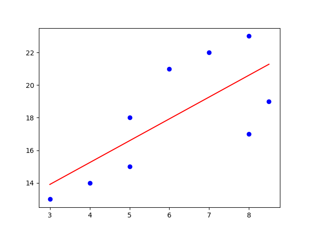

Maximum Likelihood Estimation
or MLE for short, is a function applied for parameter estimation. In MLE the loss function is represented as the log-likelihood function. Log-likelihood is used to derive the maximum likelihood of some parameter Θ (theta). We use log here because the asymptotic curve of the logarithm prevents from exploding or shirking values. Thus the sums of the values are easier to analyze.
In models, based on probability, MLE has a nice application in relation to loss functions as MLE can be used to figure out the loss function for such models. Thus, maximum likelihood estimation can be applied to select a loss function for a ML model.
You can read more about Maximum Likelihood Estimation in the end of this article .
Cross Entropy
Cross Entropy Loss (sometimes named «Log Loss» or «Negative Log Likelihood») is one of the loss functions in ML. It judges a probability output of a ML classification model, that lies between [0;1]. We normally use cross entropy as a loss function when we have the softmax activation function in the last output layer in a multi layered neural network. In case that the predicted probability continuously varies from the actual label, the cross entropy will increase. In the ideal situation the cross entropy (or log loss) is equal to zero, so the difference from the actual (ideal) label is zero (or very small).
As a rule of thumb, use the cross entropy loss with softmax.
The idea of cross entropy and entropy itself roots in the information theory which deals with the problem of reliable message transmission with zero or minimum amount of information loss. We also want only useful information, with which we can make further predictions.
In other words, entropy is a measure of practical information we receive from one data point. The entropy becomes large if the variation in the data becomes large.
Binary Cross Entropy vs Categorical Cross Entropy
Binary Cross Entropy Function :
If we have to classify only two classes, we chose binary cross entropy.
L = — Σ Nn=1 {dn log pn + (1 — dn) log(1 — pn)}
We said before that we use softmax as an activation function in the last layer. With binary cross entropy, it is advisable to use the sigmoid activation function. Feel free to read more about activation functions.
The code demonstration will be done with the help of the
Keras
ML library.
from keras.preprocessing import sequence
from keras.models import Sequential
from keras.layers import Dense, Embedding, LSTM, Bidirectional


#  this function builds, trains and evaluates a keras LSTM model

def build_and_evaluate_model(x_train, y_train, x_develop, y_develop):

    x_train = sequence.pad_sequences(x_train, maxlen = 100)
    x_dev = sequence.pad_sequences(x_develop, maxlen = 100)

    model = Sequential()
    model.add(Embedding(input_dim = 10000, output_dim = 50))  #input_dim or the size of the data set, e.g vocabulary
    model.add(Bidirectional(LSTM(units = 25)))
    model.add(Dense(1,activation='sigmoid'))
    model.predict(x_develop)
    model.compile(loss = 'binary_crossentropy', optimizer = 'adam', metrics=['accuracy'])
    model.fit(x = x_train, y = y_train, batch_size = 32, epochs = 10, validation_data = (x_develop, y_develop))

    score, acc = model.evaluate(x_develop, y_develop)

    return score, acc, model
Consider the whole code following this link to: Train a recurrent convolutional network on the IMDB sentiment classification task.
To find out more about the LSTM model used in the code above, read this article.
Categorical Cross Entropy Function :
If we have to classify multiple classes, we chose categorical cross entropy.

Categorical Cross Entropy is sometimes referred to as the softmax loss. The softmax loss is basically the softmax activation function combined with the cross entropy loss function. Essentially, it will output some probability over some N classes for each data sample.
Categorical Cross Entropy is already implemented in the Keras ML library:
keras.losses.categorical_crossentropy(y_true, y_pred, from_logits=False, label_smoothing=0) We can also use already implemented in Keras mean squared error (MSE) as our loss function. As a general rule, use a linear activation function and only one node in the output layer if MSE is used :
model.compile(loss="mse")  #instead of writing "mse", "mean_squared_error" is also acceptable and less cryptic

model.add(Dense(1, activation="linear"))
Feel free to consult the Keras official documentation .
Conclusion
To sum up, loss functions are not always easy to comprehend. In some ML cases, it is more relevant to measure and present the accuracy of classification Ml models.
Sometimes we should select other metrics than the loss functions. An important thought: one may assume that the ML model which has the minimum loss, would be the best pick, but it doesn’t have to be like this. The model with the lowest loss still can be the model with the worst metric after all.
A sufficient practice would be to apply a loss function for evaluation of the model’s learning progress. Shortly, use loss functions for optimization: analyze whether there are typical problems such as: slow convergence or over/underfitting in the model. Chose the proper metric according to the task the ML model have to accomplish and use a loss function as an optimizer for model’s performance.
Further recommended readings:
Recurrent Neural Networks (RNNs)
Partial Derivatives and the Jacobian Matrix
Usage of loss functions Keras
Machine learning: an introduction to mean squared error and regression lines
In this post, I show you how to implement the Mean Squared Error (MSE) Loss/Cost function as well as its derivative for Neural networks in Python. The function is meant for working with a batch of inputs, i.e., a batch of samples is provided at once.
The mathematical definition of the MSE loss function is
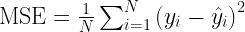
where  are the expected or target outputs (known beforehand),
  are the predicted outputs from the neural network, and
  is the number of samples.
The derivative of the MSE loss function is:
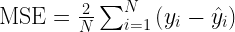
Please note, that in the above definitions we are only considering a single output node. That is there is one output per sample.
But it is very common for neural networks to have more than one output node (multiple outputs) for a given input. In that case one has to average the squared error not only over the samples but also over the number of output nodes.
In this post I will only focus on this general case which means we would expect the predicted and target outputs to be 2D arrays, with nRows=nSamples, and nColumns=nOutput_Nodes. In other words, the rows correspond to outputs for different set of input samples, and the columns correspond to the outputs from the different output nodes.
Based on this we can implement the MSE loss function in Python as:
MSE loss simplest implementation
def MSE_loss(predictions, targets):
    """
    Computes Mean Squared error/loss between targets
    and predictions.
    Input: predictions (N, k) ndarray (N: no. of samples, k: no. of output nodes)
          targets (N, k) ndarray        (N: no. of samples, k: no. of output nodes)
    Returns: scalar
    Note: The averaging is only done over the output nodes and not over the samples in a batch.
    Therefore, to get an answer similar to PyTorch, one must divide the result by the batch size.
    """

    return np.sum((predictions-targets**2)/predictions.shape[1]
MSE loss derivative simplest implementation
def MSE_loss_grad(predictions, targets):
    """
    Computes mean squared error gradient between targets
    and predictions.
    Input: predictions (N, k) ndarray (N: no. of samples, k: no. of output nodes)
          targets (N, k) ndarray        (N: no. of samples, k: no. of output nodes)
    Returns: (N,k) ndarray
    Note: The averaging is only done over the output nodes and not over the samples in a batch.
    Therefore, to get an answer similar to PyTorch, one must divide the result by the batch size.
    """

    return 2*(predictions-targets)/predictions.shape[1]
The above functions return the MSE loss and its derivative respectively, only averaged over the output nodes. Averaging over the samples can then be done by simply dividing the result by nSamples as shown
average_MSE = MSE_loss(predictions, target)/predictions.shape[0]
average_MSE_grad = MSE_loss_grad(predictions, target)/predictions.shape[0]
These implementations can be further accelerated (sped-up) by using Numba (https://numba.pydata.org/). Numba is a Just-in-time (JIT) compiler that
translates a subset of Python and NumPy code into fast machine code.
To use numba, install it as:
pip install numba
Also, make sure that your numpy is compatible with Numba or not, although usually pip takes care of that. You can get the info here: https://pypi.org/project/numba/
Accelerating the above functions using Numba is quite simple. Just modify them in the following manner:
MSE loss NUMBA implementation
from numba import njit
@njit(cache=True,fastmath=True)
def MSE_loss(predictions, targets):
    """
    Computes Mean Squared error/loss between targets
    and predictions.
    Input: predictions (N, k) ndarray (N: no. of samples, k: no. of output nodes)
          targets (N, k) ndarray        (N: no. of samples, k: no. of output nodes)
    Returns: scalar
    Note: The averaging is only done over the output nodes and not over the samples in a batch.
    Therefore, to get an answer similar to PyTorch, one must divide the result by the batch size.
    """

    return np.sum((predictions-targets)**2)/predictions.shape[1]
NOTE: I noticed that the above implementation can be unstable and return erroneous results for very large arrays. Therefore, you can use the following even faster implementation with parallelization:
from numba import njit
@njit(cache=True,fastmath=False, parallel=True)
def MSE_loss(predictions, targets):
    """
    Computes Mean Squared error/loss between targets
    and predictions.
    Input: predictions (N, k) ndarray (N: no. of samples, k: no. of output nodes)
          targets (N, k) ndarray        (N: no. of samples, k: no. of output nodes)
    Returns: scalar
    Note: The averaging is only done over the output nodes and not over the samples in a batch.
    Therefore, to get an answer similar to PyTorch, one must divide the result by the batch size.
    """
    loss = 0.0
    for i in prange(predictions.shape[0]):
        for j in range(predictions.shape[1]):
            loss = loss + (predictions[i,j] - targets[i,j])**2
    # Average over number of output nodes
    loss = loss / predictions.shape[1]
    return loss
MSE loss derivative NUMBA implementation
from numba import njit
@njit(cache=True,fastmath=True)
def MSE_loss_grad(predictions, targets):
    """
    Computes mean squared error gradient between targets
    and predictions.
    Input: predictions (N, k) ndarray (N: no. of samples, k: no. of output nodes)
          targets (N, k) ndarray        (N: no. of samples, k: no. of output nodes)
    Returns: (N,k) ndarray
    Note: The averaging is only done over the output nodes and not over the samples in a batch.
    Therefore, to get an answer similar to PyTorch, one must divide the result by the batch size.
    """

    return 2*(predictions-targets)/predictions.shape[1]
This is quite fast and competitive with Tensorflow and PyTorch.
It is in fact also used in the CrysX-Neural Network library (crysx_nn)
Furthermore, the above implementations can also be accelerated using Cupy (CUDA).
CuPy is an open-source array library for GPU-accelerated computing with Python. CuPy utilizes CUDA Toolkit libraries to make full use of the GPU architecture.
The Cupy implementations look as follows:
def MSE_loss_cupy(predictions, targets):
    """
    Computes Mean Squared error/loss between targets
    and predictions.
    Input: predictions (N, k) ndarray (N: no. of samples, k: no. of output nodes)
          targets (N, k) ndarray        (N: no. of samples, k: no. of output nodes)
    Returns: scalar
    Note: The averaging is only done over the output nodes and not over the samples in a batch.
    Therefore, to get an answer similar to PyTorch, one must divide the result by the batch size.
    """

    return cp.sum((predictions-targets)**2)/predictions.shape[1]
def MSE_loss_grad_cupy(predictions, targets):
    """
    Computes mean squared error gradient between targets
    and predictions.
    Input: predictions (N, k) ndarray (N: no. of samples, k: no. of output nodes)
          targets (N, k) ndarray        (N: no. of samples, k: no. of output nodes)
    Returns: (N,k) ndarray
    Note: The averaging is only done over the output nodes and not over the samples in a batch.
    Therefore, to get an answer similar to PyTorch, one must divide the result by the batch size.
    """

    return 2*(predictions-targets)/predictions.shape[1]
The above code is also used in the crysx_nn library.
I hope you found this information useful.
If you did, then don’t forget to check out my other posts on Machine Learning and efficient implementations of activation/loss functions in Python.

Ph.D. researcher at Friedrich-Schiller University Jena, Germany. I’m a physicist specializing in computational material science. I write efficient codes for simulating light-matter interactions at atomic scales. I like to develop Physics, DFT, and Machine Learning related apps and software from time to time. Can code in most of the popular languages. I like to share my knowledge in Physics and applications using this Blog and a YouTube channel.
[wpedon id=»7041″ align=»center»]
Before we discuss different kinds of loss functions used in deep learning, let’s talk about why we need loss functions in the first place. To do that, we first need to learn about what’s happening inside a neural network.
More From Artem OppermannArtificial Intelligence vs. Machine Learning vs. Deep Learning
Why Do We Need Loss Functions in Deep Learning?
There are two possible mathematical operations happening inside a neural network:
-
Forward propagation
-
Backpropagation with gradient descent
While forward propagation refers to the computational process of predicting an output for a given input vector x, backpropagation and gradient descent describe the process of improving the weights and biases of the network in order to make better predictions. Let’s look at this in practice.
For a given input vector x the neural network predicts an output, which is generally called a prediction vector y.
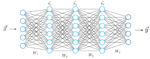
The equations describing the mathematics happening during the prediction vector’s computation looks like this:
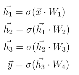
We must compute a dot-product between the input vector x and the weight matrix W1 that connects the first layer with the second. After that, we apply a non-linear activation function to the result of the dot-product.
What Are Loss Functions?
- A loss function measures how good a neural network model is in performing a certain task, which in most cases is regression or classification.
- We must minimize the value of the loss function during the backpropagation step in order to make the neural network better.
- We only use the cross-entropy loss function in classification tasks when we want the neural network to predict probabilities.
- For regression tasks, when we want the network to predict continuous numbers, we must use the mean squared error loss function.
- We use mean absolute percentage error loss function during demand forecasting to keep an eye on the performance of the network during training time.
The prediction vector can represent a number of things depending on the task we want the network to do. For regression tasks, which are basically predictions of continuous variables (e.g. stock price, expected demand for products, etc.), the output vector y contains continuous numbers.
Regardless of the task, we somehow have to measure how close our predictions are to the ground truth label.
On the other hand, for classification tasks, such as customer segmentation or image classification, the output vector y represents probability scores between 0.0 and 1.0.
The value we want the neural network to predict is called a ground truth label, which is usually represented as y_hat. A predicted value y closer to the label suggests a better performance of the neural network.
Regardless of the task, we somehow have to measure how close our predictions are to the ground truth label.
This is where the concept of a loss function comes into play.
Mathematically, we can measure the difference (or error) between the prediction vector y and the label y_hat by defining a loss function whose value depends on this difference.
An example of a general loss function is the quadratic loss:
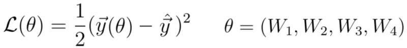
Since the prediction vector y(θ) is a function of the neural network’s weights (which we abbreviate to θ), the loss is also a function of the weights.
Since the loss depends on weights, we must find a certain set of weights for which the value of the loss function is as small as possible. We achieve this mathematically through a method called gradient descent.
The value of this loss function depends on the difference between the label y_hat and y. A higher difference means a higher loss value while (you guessed it) a smaller difference means a smaller loss value. Minimizing the loss function directly leads to more accurate predictions of the neural network as the difference between the prediction and the label decreases.
The neural network’s only objective is to minimize the loss function.
In fact, the neural network’s only objective is to minimize the loss function. This is because minimizing the loss function automatically causes the neural network model to make better predictions regardless of the exact characteristics of the task at hand.
A neural network solves tasks without being explicitly programmed with a task-specific rule. This is possible because the goal of minimizing the loss function is universal and doesn’t depend on the task or circumstances.
3 Key Types of Loss Functions in Neural Networks
That said, you still have to select the right loss function for the task at hand. Luckily there are only three loss functions you need to know to solve almost any problem.
3 Key Loss Functions
- Mean Squared Error Loss Function
- Cross-Entropy Loss Function
- Mean Absolute Percentage Error
1. Mean Squared Error Loss Function
Mean squared error (MSE) loss function is the sum of squared differences between the entries in the prediction vector y and the ground truth vector y_hat.
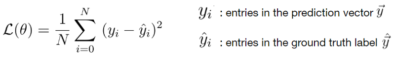
You divide the sum of squared differences by N, which corresponds to the length of the vectors. If the output y of your neural network is a vector with multiple entries then N is the number of the vector entries with y_i being one particular entry in the output vector.
The mean squared error loss function is the perfect loss function if you’re dealing with a regression problem. That is, if you want your neural network to predict a continuous scalar value.
An example of a regression problem would be predictions of . . .
-
the number of products needed in a supply chain.
-
future real estate prices under certain market conditions.
-
a stock value.
Here is a code snippet where I’ve calculated MSE loss in Python:
import numpy as np

# The prediction vector of the neural network
y_pred=[0.6, 1.29, 1.99, 2.69, 3.4]

# The ground truth label
y_hat= [1, 1, 2, 2, 4]

# Mean squared error
MSE = np.sum(np.square(np.subtract(y_hat, y_pred)))/len(y_hat)

print(MSE) # The result is 0.21606
Learn More From Our ExpertsWhat Is Linear Regression?
2. Cross-Entropy Loss Function
Regression is only one of two areas where feedforward networks enjoy great popularity. The other area is classification.
In classification tasks, we deal with predictions of probabilities, which means the output of a neural network must be in a range between zero and one. A loss function that can measure the error between a predicted probability and the label which represents the actual class is called the cross-entropy loss function.
One important thing we need to discuss before continuing with the cross-entropy is what exactly the ground truth vector looks like in the case of a classification problem.
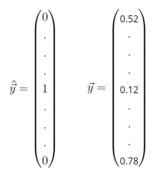
The label vector y_hat is one hot encoded which means the values in this vector can only take discrete values of either zero or one. The entries in this vector represent different classes. The values of these entries are zero, except for a single entry which is one. This entry tells us the class into which we want to classify the input feature vector x.
The prediction y, however, can take continuous values between zero and one.
Given the prediction vector y and the ground truth vector y_hat you can compute the cross-entropy loss between those two vectors as follows:
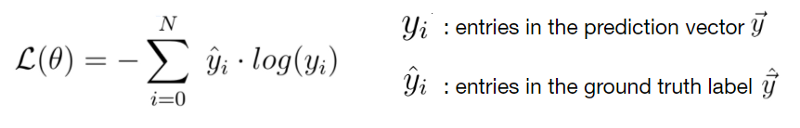
First, we need to sum up the products between the entries of the label vector y_hat and the logarithms of the entries of the predictions vector y. Then we must negate the sum to get a positive value of the loss function.
One interesting thing to consider is the plot of the cross-entropy loss function. In the following graph, you can see the value of the loss function (y-axis) vs. the predicted probability y_i. Here y_i takes values between zero and one.
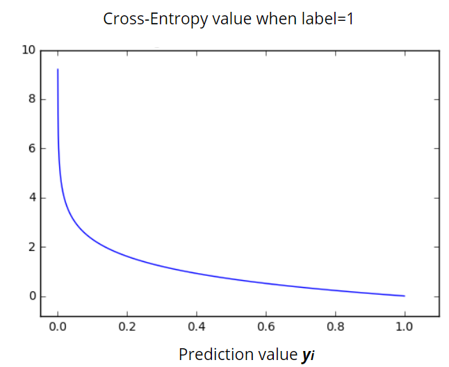
We can see clearly that the cross-entropy loss function grows exponentially for lower values of the predicted probability y_i. For y_i=0 the function becomes infinite, while for y_i=1 the neural network makes an accurate probability prediction and the loss value goes to zero.
Here’s another code snippet in Python where I’ve calculated the cross-entropy loss function:
import numpy as np

# The probabilities predicted by the neural network
y_pred = [0.1, 0.3, 0.4, 0.2]

# one-hot-encoded ground truth label
y_hat =[0, 1, 0, 0]

cross_entropy = - np.sum(np.log(y_pred)*y_hat)

print(cross_entropy) # The Result is 1.20
Read More From Our Machine Learning ExpertsMachine Learning for Beginners
3. Mean Absolute Percentage Error
Finally, we come to the Mean Absolute Percentage Error (MAPE) loss function. This loss function doesn’t get much attention in deep learning. For the most part, we use it to measure the performance of a neural network during demand forecasting tasks.
First thing first: what is demand forecasting?
Demand forecasting is the area of predictive analytics dedicated to predicting the expected demand for a good or service in the near future. For example:
-
In retail, we can use demand forecasting models to determine the amount of a particular product that should be available and at what price.
-
In industrial manufacturing, we can predict how much of each product should be produced, the amount of stock that should be available at various points in time, and when maintenance should be performed.
-
In the travel and tourism industry, we can use demand forecasting models to assess optimal price points for flights and hotels, in light of available capacity, what price should be assigned (for hotels, flights), which destinations should be spotlighted, or, what types of packages should be advertised.
Although demand forecasting is also a regression task and the minimization of the MSE loss function is an adequate training goal, this type of loss function to measure the performance of the model during training isn’t suitable for demand forecasting.
Why is that?
Well, imagine the MSE loss function gives you a value of 100. Can you tell if this is generally a good result? No, because it depends on the situation. If the prediction y of the model is 1000 and the actual ground truth label y_hat is 1010, then the MSE loss of 100 would be in fact a very small error and the performance of the model would be quite good.
However in the case where the prediction would be five and the label is 15, you would have the same loss value of 100 but the relative deviation to the ground-truth value would be much higher than in the previous case.
This example shows the shortcoming of the mean squared error function as the loss function for the demand forecasting models. For this reason, I strongly recommend using mean absolute percentage error (MAPE).
The mean absolute percentage error, also known as mean absolute percentage deviation (MAPD) usually expresses accuracy as a percentage. We define it with the following equation:
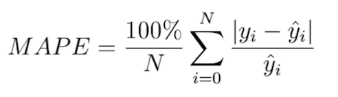
In this equation, y_i is the predicted value and y_hat is the label. We divide the difference between y_i and y_hat by the actual value y_hat again. Finally, multiplying by 100 percent gives us the percentage error.
Applying this equation to the example above gives you a more meaningful understanding of the model’s performance. In the first case, the deviation from the ground truth label would be only one percent, while in the second case the deviation would be 66 percent:
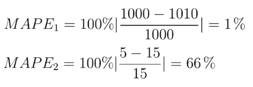
We see that the performance of these two models is very different. Meanwhile, the MSE loss function would indicate that the performance of both models is the same.
The following Python code snipped shows how we can calculate MAPE:
ximport numpy as np

# The prediction vector of the neural network
y_pred=[0.6, 1.29, 1.99, 2.69, 3.4]

# The ground truth label
y_hat= [1, 1, 2, 2, 4]

MAPE = (100.0/len(y_hat))*np.sum(np.abs(y_pred-y_hat)/y_hat)

print(MAPE) # The result is mean percentage error of 23.79%
Best Practices for Loss Functions and Neural Networks
When you’re working with loss functions, just remember these key principles:
-
A loss function measures how good a neural network model is in performing a certain task, which in most cases is regression or classification.
-
We must minimize the value of the loss function during the backpropagation step in order to make the neural network better.
-
We only use the cross-entropy loss function in classification tasks when we want the neural network to predict probabilities.
-
For regression tasks, when we want the network to predict continuous numbers, we must use the mean squared error loss function.
-
We use mean absolute percentage error loss function during demand forecasting to keep an eye on the performance of the network during training time.
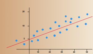
In this post, you will be learning the difference between two common types of loss functions: Cross-Entropy Loss and Mean Squared Error (MSE) Loss. These are both used in machine learning for classification & regression tasks, respecitively, to measure how well a model performs on unseen dataset. Both these losses are ways of measuring how well the predictions are made by classification and regression algorithms, and they both provide different information about the performance of models. As a data scientist, it is very important for you to understand the difference between loss functions in a great manner.
What is cross-entropy loss?
Cross entropy loss is used in classification tasks where we are trying to minimize the probability of a negative class by maximizing an expected value of some function on our training data, also called as “loss function”. Simply speaking, it is used to measure the difference between two probabilities that a model assigns to classes. Cross entropy loss is also called as ‘softmax loss’ after the predefined function in neural networks. It is also used for multi-class classification problems. An example of the usage of cross-entropy loss for multi-class classification problems is training the model using MNIST dataset. The idea of this loss function is to give a high penalty for wrong predictions and a low penalty for correct classifications. It calculates a probability that each sample belongs to one of the classes, then it uses cross-entropy between these probabilities as its cost function. The more confident model is about prediction, the less penalty it incurs.
Cross-entropy loss is very similar to cross entropy. They both measure the difference between an actual probability and predicted probability, but cross entropy uses log probabilities while cross-entropy loss uses negative log probabilities (which are then multiplied by -log(p)) . Log probabilities can be converted into regular numbers for ease of computation using a softmax function.
Cross-entropy loss is also used in time series classification problems such as forecasting weather or stock values. An example would be comparing the forecast of a short term vs long term prediction model making cross-entropy loss incurring large penalty when one class has much higher probability.
A common example used to understand cross-entropy loss is comparing apples and oranges where each fruit has a certain probability of being chosen out of three probabilities (apple, orange, or other). Apple would have an 80% chance while Oranges will only get 20%. In order for our model to make correct predictions in this example, it should assign a high probability to apple and a low for orange. If cross-entropy loss is used, we can compute the cross-entropy loss for each fruit and assign probabilities accordingly. We will then want to choose apple with a higher probability as it has less cross entropy lost than oranges.
How do you calculate cross-entropy loss?
Cross-entropy loss is calculated by taking the difference between our prediction and actual output. We then multiply that value with `-y * ln(y)`. This means we take a negative number, raise it to the power of the logarithm of y (which will be positive), and then subtract this from our original calculation.
Here is the formula for calculating cross entropy loss:
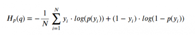
The cross entropy loss is then calculated by using the cross-entropy formula and adding up all the losses: C = sum_{i=0}^{m} cross_entropy(X, Y)
What is mean squared error (MSE) loss?
Mean squared error (MSE) loss is used in regression tasks where we are trying to minimize an expected value of some function on our training data, which is also called as “loss function”.
How do you calculate mean squared error loss?
Mean squared error (MSE) loss is calculated by taking the difference between `y` and our prediction, then square those values. We take these new numbers (square them), add all of that together to get a final value, finally divide this number by y again. This will be our final result.
The formula for calculating mean squared error loss is as follows:
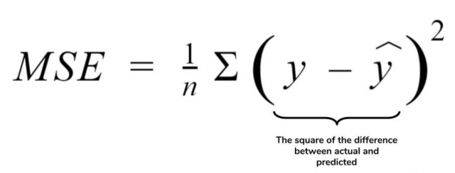
This will give us a loss value between 0 and infinity with larger values indicating mean squared error.
Root mean square error (RMSE) is a mean square error loss function that is normalized between 0 and infinity. The root mean squared error (RMSE) can be written as follows:
$$RMSE = sqrt{frac{ mean_squared_error}{m}}$$
- Author
- Recent Posts

I have been recently working in the area of Data analytics including Data Science and Machine Learning / Deep Learning. I am also passionate about different technologies including programming languages such as Java/JEE, Javascript, Python, R, Julia, etc, and technologies such as Blockchain, mobile computing, cloud-native technologies, application security, cloud computing platforms, big data, etc. For latest updates and blogs, follow us on Twitter. I would love to connect with you on Linkedin.
Check out my latest book titled as First Principles Thinking: Building winning products using first principles thinking

Ajitesh Kumar
I have been recently working in the area of Data analytics including Data Science and Machine Learning / Deep Learning. I am also passionate about different technologies including programming languages such as Java/JEE, Javascript, Python, R, Julia, etc, and technologies such as Blockchain, mobile computing, cloud-native technologies, application security, cloud computing platforms, big data, etc. For latest updates and blogs, follow us on Twitter. I would love to connect with you on Linkedin.
Check out my latest book titled as First Principles Thinking: Building winning products using first principles thinking