From Wikipedia, the free encyclopedia
In statistics, the mean squared error (MSE)[1] or mean squared deviation (MSD) of an estimator (of a procedure for estimating an unobserved quantity) measures the average of the squares of the errors—that is, the average squared difference between the estimated values and the actual value. MSE is a risk function, corresponding to the expected value of the squared error loss.[2] The fact that MSE is almost always strictly positive (and not zero) is because of randomness or because the estimator does not account for information that could produce a more accurate estimate.[3] In machine learning, specifically empirical risk minimization, MSE may refer to the empirical risk (the average loss on an observed data set), as an estimate of the true MSE (the true risk: the average loss on the actual population distribution).
The MSE is a measure of the quality of an estimator. As it is derived from the square of Euclidean distance, it is always a positive value that decreases as the error approaches zero.
The MSE is the second moment (about the origin) of the error, and thus incorporates both the variance of the estimator (how widely spread the estimates are from one data sample to another) and its bias (how far off the average estimated value is from the true value).[citation needed] For an unbiased estimator, the MSE is the variance of the estimator. Like the variance, MSE has the same units of measurement as the square of the quantity being estimated. In an analogy to standard deviation, taking the square root of MSE yields the root-mean-square error or root-mean-square deviation (RMSE or RMSD), which has the same units as the quantity being estimated; for an unbiased estimator, the RMSE is the square root of the variance, known as the standard error.
Definition and basic properties[edit]
The MSE either assesses the quality of a predictor (i.e., a function mapping arbitrary inputs to a sample of values of some random variable), or of an estimator (i.e., a mathematical function mapping a sample of data to an estimate of a parameter of the population from which the data is sampled). The definition of an MSE differs according to whether one is describing a predictor or an estimator.
Predictor[edit]
If a vector of  predictions is generated from a sample of data points on all variables, and
  is the vector of observed values of the variable being predicted, with
  being the predicted values (e.g. as from a least-squares fit), then the within-sample MSE of the predictor is computed as

In other words, the MSE is the mean  of the squares of the errors
  . This is an easily computable quantity for a particular sample (and hence is sample-dependent).
In matrix notation,

where  is
is  and
and  is the
  column vector.
The MSE can also be computed on q data points that were not used in estimating the model, either because they were held back for this purpose, or because these data have been newly obtained. Within this process, known as statistical learning, the MSE is often called the test MSE,[4] and is computed as

Estimator[edit]
The MSE of an estimator  with respect to an unknown parameter
  is defined as[1]
![{displaystyle operatorname {MSE} ({hat {theta }})=operatorname {E} _{theta }left[({hat {theta }}-theta )^{2}right].}](https://wikimedia.org/api/rest_v1/media/math/render/svg/9a0e1b3bac58f9ba2d2f4ff8b85b2e35a8f4bf78)
This definition depends on the unknown parameter, but the MSE is a priori a property of an estimator. The MSE could be a function of unknown parameters, in which case any estimator of the MSE based on estimates of these parameters would be a function of the data (and thus a random variable). If the estimator is derived as a sample statistic and is used to estimate some population parameter, then the expectation is with respect to the sampling distribution of the sample statistic.
The MSE can be written as the sum of the variance of the estimator and the squared bias of the estimator, providing a useful way to calculate the MSE and implying that in the case of unbiased estimators, the MSE and variance are equivalent.[5]

Proof of variance and bias relationship[edit]
![{displaystyle {begin{aligned}operatorname {MSE} ({hat {theta }})&=operatorname {E} _{theta }left[({hat {theta }}-theta )^{2}right]\&=operatorname {E} _{theta }left[left({hat {theta }}-operatorname {E} _{theta }[{hat {theta }}]+operatorname {E} _{theta }[{hat {theta }}]-theta right)^{2}right]\&=operatorname {E} _{theta }left[left({hat {theta }}-operatorname {E} _{theta }[{hat {theta }}]right)^{2}+2left({hat {theta }}-operatorname {E} _{theta }[{hat {theta }}]right)left(operatorname {E} _{theta }[{hat {theta }}]-theta right)+left(operatorname {E} _{theta }[{hat {theta }}]-theta right)^{2}right]\&=operatorname {E} _{theta }left[left({hat {theta }}-operatorname {E} _{theta }[{hat {theta }}]right)^{2}right]+operatorname {E} _{theta }left[2left({hat {theta }}-operatorname {E} _{theta }[{hat {theta }}]right)left(operatorname {E} _{theta }[{hat {theta }}]-theta right)right]+operatorname {E} _{theta }left[left(operatorname {E} _{theta }[{hat {theta }}]-theta right)^{2}right]\&=operatorname {E} _{theta }left[left({hat {theta }}-operatorname {E} _{theta }[{hat {theta }}]right)^{2}right]+2left(operatorname {E} _{theta }[{hat {theta }}]-theta right)operatorname {E} _{theta }left[{hat {theta }}-operatorname {E} _{theta }[{hat {theta }}]right]+left(operatorname {E} _{theta }[{hat {theta }}]-theta right)^{2}&&operatorname {E} _{theta }[{hat {theta }}]-theta ={text{const.}}\&=operatorname {E} _{theta }left[left({hat {theta }}-operatorname {E} _{theta }[{hat {theta }}]right)^{2}right]+2left(operatorname {E} _{theta }[{hat {theta }}]-theta right)left(operatorname {E} _{theta }[{hat {theta }}]-operatorname {E} _{theta }[{hat {theta }}]right)+left(operatorname {E} _{theta }[{hat {theta }}]-theta right)^{2}&&operatorname {E} _{theta }[{hat {theta }}]={text{const.}}\&=operatorname {E} _{theta }left[left({hat {theta }}-operatorname {E} _{theta }[{hat {theta }}]right)^{2}right]+left(operatorname {E} _{theta }[{hat {theta }}]-theta right)^{2}\&=operatorname {Var} _{theta }({hat {theta }})+operatorname {Bias} _{theta }({hat {theta }},theta )^{2}end{aligned}}}](https://wikimedia.org/api/rest_v1/media/math/render/svg/2ac524a751828f971013e1297a33ca1cc4c38cd6)
An even shorter proof can be achieved using the well-known formula that for a random variable  ,
,  . By substituting with,
  , we have
![{displaystyle {begin{aligned}operatorname {MSE} ({hat {theta }})&=mathbb {E} [({hat {theta }}-theta )^{2}]\&=operatorname {Var} ({hat {theta }}-theta )+(mathbb {E} [{hat {theta }}-theta ])^{2}\&=operatorname {Var} ({hat {theta }})+operatorname {Bias} ^{2}({hat {theta }})end{aligned}}}](https://wikimedia.org/api/rest_v1/media/math/render/svg/864646cf4426e2b62a3caf9460382eec1a77fe4e)
But in real modeling case, MSE could be described as the addition of model variance, model bias, and irreducible uncertainty (see Bias–variance tradeoff). According to the relationship, the MSE of the estimators could be simply used for the efficiency comparison, which includes the information of estimator variance and bias. This is called MSE criterion.
In regression[edit]
In regression analysis, plotting is a more natural way to view the overall trend of the whole data. The mean of the distance from each point to the predicted regression model can be calculated, and shown as the mean squared error. The squaring is critical to reduce the complexity with negative signs. To minimize MSE, the model could be more accurate, which would mean the model is closer to actual data. One example of a linear regression using this method is the least squares method—which evaluates appropriateness of linear regression model to model bivariate dataset,[6] but whose limitation is related to known distribution of the data.
The term mean squared error is sometimes used to refer to the unbiased estimate of error variance: the residual sum of squares divided by the number of degrees of freedom. This definition for a known, computed quantity differs from the above definition for the computed MSE of a predictor, in that a different denominator is used. The denominator is the sample size reduced by the number of model parameters estimated from the same data, (n−p) for p regressors or (n−p−1) if an intercept is used (see errors and residuals in statistics for more details).[7] Although the MSE (as defined in this article) is not an unbiased estimator of the error variance, it is consistent, given the consistency of the predictor.
In regression analysis, «mean squared error», often referred to as mean squared prediction error or «out-of-sample mean squared error», can also refer to the mean value of the squared deviations of the predictions from the true values, over an out-of-sample test space, generated by a model estimated over a particular sample space. This also is a known, computed quantity, and it varies by sample and by out-of-sample test space.
Examples[edit]
Mean[edit]
Suppose we have a random sample of size from a population,  . Suppose the sample units were chosen with replacement. That is, the units are selected one at a time, and previously selected units are still eligible for selection for all draws. The usual estimator for the
  is the sample average

which has an expected value equal to the true mean (so it is unbiased) and a mean squared error of
![{displaystyle operatorname {MSE} left({overline {X}}right)=operatorname {E} left[left({overline {X}}-mu right)^{2}right]=left({frac {sigma }{sqrt {n}}}right)^{2}={frac {sigma ^{2}}{n}}}](https://wikimedia.org/api/rest_v1/media/math/render/svg/b4647a2cc4c8f9a4c90b628faad2dcf80c4aae84)
where  is the population variance.
For a Gaussian distribution, this is the best unbiased estimator (i.e., one with the lowest MSE among all unbiased estimators), but not, say, for a uniform distribution.
Variance[edit]
The usual estimator for the variance is the corrected sample variance:

This is unbiased (its expected value is ), hence also called the unbiased sample variance, and its MSE is[8]

where  is the fourth central moment of the distribution or population, and
  is the excess kurtosis.
However, one can use other estimators for which are proportional to  , and an appropriate choice can always give a lower mean squared error. If we define

then we calculate:
![{displaystyle {begin{aligned}operatorname {MSE} (S_{a}^{2})&=operatorname {E} left[left({frac {n-1}{a}}S_{n-1}^{2}-sigma ^{2}right)^{2}right]\&=operatorname {E} left[{frac {(n-1)^{2}}{a^{2}}}S_{n-1}^{4}-2left({frac {n-1}{a}}S_{n-1}^{2}right)sigma ^{2}+sigma ^{4}right]\&={frac {(n-1)^{2}}{a^{2}}}operatorname {E} left[S_{n-1}^{4}right]-2left({frac {n-1}{a}}right)operatorname {E} left[S_{n-1}^{2}right]sigma ^{2}+sigma ^{4}\&={frac {(n-1)^{2}}{a^{2}}}operatorname {E} left[S_{n-1}^{4}right]-2left({frac {n-1}{a}}right)sigma ^{4}+sigma ^{4}&&operatorname {E} left[S_{n-1}^{2}right]=sigma ^{2}\&={frac {(n-1)^{2}}{a^{2}}}left({frac {gamma _{2}}{n}}+{frac {n+1}{n-1}}right)sigma ^{4}-2left({frac {n-1}{a}}right)sigma ^{4}+sigma ^{4}&&operatorname {E} left[S_{n-1}^{4}right]=operatorname {MSE} (S_{n-1}^{2})+sigma ^{4}\&={frac {n-1}{na^{2}}}left((n-1)gamma _{2}+n^{2}+nright)sigma ^{4}-2left({frac {n-1}{a}}right)sigma ^{4}+sigma ^{4}end{aligned}}}](https://wikimedia.org/api/rest_v1/media/math/render/svg/cf22322412b8454c706d78671e5d94208675a6e0)
This is minimized when

For a Gaussian distribution, where  , this means that the MSE is minimized when dividing the sum by
  . The minimum excess kurtosis is
  ,[a] which is achieved by a Bernoulli distribution with p = 1/2 (a coin flip), and the MSE is minimized for
  Hence regardless of the kurtosis, we get a «better» estimate (in the sense of having a lower MSE) by scaling down the unbiased estimator a little bit; this is a simple example of a shrinkage estimator: one «shrinks» the estimator towards zero (scales down the unbiased estimator).
Further, while the corrected sample variance is the best unbiased estimator (minimum mean squared error among unbiased estimators) of variance for Gaussian distributions, if the distribution is not Gaussian, then even among unbiased estimators, the best unbiased estimator of the variance may not be 
Gaussian distribution[edit]
The following table gives several estimators of the true parameters of the population, μ and σ2, for the Gaussian case.[9]
| True value | Estimator | Mean squared error |
|---|---|---|
 |
= the unbiased estimator of the population mean,  |

|
 |
= the unbiased estimator of the population variance,  |

|
|
= the biased estimator of the population variance,  |

|
|
= the biased estimator of the population variance,  |

|
Interpretation[edit]
An MSE of zero, meaning that the estimator predicts observations of the parameter with perfect accuracy, is ideal (but typically not possible).
Values of MSE may be used for comparative purposes. Two or more statistical models may be compared using their MSEs—as a measure of how well they explain a given set of observations: An unbiased estimator (estimated from a statistical model) with the smallest variance among all unbiased estimators is the best unbiased estimator or MVUE (Minimum-Variance Unbiased Estimator).
Both analysis of variance and linear regression techniques estimate the MSE as part of the analysis and use the estimated MSE to determine the statistical significance of the factors or predictors under study. The goal of experimental design is to construct experiments in such a way that when the observations are analyzed, the MSE is close to zero relative to the magnitude of at least one of the estimated treatment effects.
In one-way analysis of variance, MSE can be calculated by the division of the sum of squared errors and the degree of freedom. Also, the f-value is the ratio of the mean squared treatment and the MSE.
MSE is also used in several stepwise regression techniques as part of the determination as to how many predictors from a candidate set to include in a model for a given set of observations.
Applications[edit]
- Minimizing MSE is a key criterion in selecting estimators: see minimum mean-square error. Among unbiased estimators, minimizing the MSE is equivalent to minimizing the variance, and the estimator that does this is the minimum variance unbiased estimator. However, a biased estimator may have lower MSE; see estimator bias.
- In statistical modelling the MSE can represent the difference between the actual observations and the observation values predicted by the model. In this context, it is used to determine the extent to which the model fits the data as well as whether removing some explanatory variables is possible without significantly harming the model’s predictive ability.
- In forecasting and prediction, the Brier score is a measure of forecast skill based on MSE.
Loss function[edit]
Squared error loss is one of the most widely used loss functions in statistics[citation needed], though its widespread use stems more from mathematical convenience than considerations of actual loss in applications. Carl Friedrich Gauss, who introduced the use of mean squared error, was aware of its arbitrariness and was in agreement with objections to it on these grounds.[3] The mathematical benefits of mean squared error are particularly evident in its use at analyzing the performance of linear regression, as it allows one to partition the variation in a dataset into variation explained by the model and variation explained by randomness.
Criticism[edit]
The use of mean squared error without question has been criticized by the decision theorist James Berger. Mean squared error is the negative of the expected value of one specific utility function, the quadratic utility function, which may not be the appropriate utility function to use under a given set of circumstances. There are, however, some scenarios where mean squared error can serve as a good approximation to a loss function occurring naturally in an application.[10]
Like variance, mean squared error has the disadvantage of heavily weighting outliers.[11] This is a result of the squaring of each term, which effectively weights large errors more heavily than small ones. This property, undesirable in many applications, has led researchers to use alternatives such as the mean absolute error, or those based on the median.
See also[edit]
- Bias–variance tradeoff
- Hodges’ estimator
- James–Stein estimator
- Mean percentage error
- Mean square quantization error
- Mean square weighted deviation
- Mean squared displacement
- Mean squared prediction error
- Minimum mean square error
- Minimum mean squared error estimator
- Overfitting
- Peak signal-to-noise ratio
Notes[edit]
- ^ This can be proved by Jensen’s inequality as follows. The fourth central moment is an upper bound for the square of variance, so that the least value for their ratio is one, therefore, the least value for the excess kurtosis is −2, achieved, for instance, by a Bernoulli with p=1/2.
References[edit]
- ^ a b «Mean Squared Error (MSE)». www.probabilitycourse.com. Retrieved 2020-09-12.
- ^ Bickel, Peter J.; Doksum, Kjell A. (2015). Mathematical Statistics: Basic Ideas and Selected Topics. Vol. I (Second ed.). p. 20.
If we use quadratic loss, our risk function is called the mean squared error (MSE) …
- ^ a b Lehmann, E. L.; Casella, George (1998). Theory of Point Estimation (2nd ed.). New York: Springer. ISBN 978-0-387-98502-2. MR 1639875.
- ^ Gareth, James; Witten, Daniela; Hastie, Trevor; Tibshirani, Rob (2021). An Introduction to Statistical Learning: with Applications in R. Springer. ISBN 978-1071614174.
- ^ Wackerly, Dennis; Mendenhall, William; Scheaffer, Richard L. (2008). Mathematical Statistics with Applications (7 ed.). Belmont, CA, USA: Thomson Higher Education. ISBN 978-0-495-38508-0.
- ^ A modern introduction to probability and statistics : understanding why and how. Dekking, Michel, 1946-. London: Springer. 2005. ISBN 978-1-85233-896-1. OCLC 262680588.
{{cite book}}: CS1 maint: others (link) - ^ Steel, R.G.D, and Torrie, J. H., Principles and Procedures of Statistics with Special Reference to the Biological Sciences., McGraw Hill, 1960, page 288.
- ^ Mood, A.; Graybill, F.; Boes, D. (1974). Introduction to the Theory of Statistics (3rd ed.). McGraw-Hill. p. 229.
- ^ DeGroot, Morris H. (1980). Probability and Statistics (2nd ed.). Addison-Wesley.
- ^ Berger, James O. (1985). «2.4.2 Certain Standard Loss Functions». Statistical Decision Theory and Bayesian Analysis (2nd ed.). New York: Springer-Verlag. p. 60. ISBN 978-0-387-96098-2. MR 0804611.
- ^ Bermejo, Sergio; Cabestany, Joan (2001). «Oriented principal component analysis for large margin classifiers». Neural Networks. 14 (10): 1447–1461. doi:10.1016/S0893-6080(01)00106-X. PMID 11771723.
From Wikipedia, the free encyclopedia
In statistics the mean squared prediction error or mean squared error of the predictions of a smoothing or curve fitting procedure is the expected value of the squared difference between the fitted values implied by the predictive function  and the values of the (unobservable) function g. It is an inverse measure of the explanatory power of
  and can be used in the process of cross-validation of an estimated model.
If the smoothing or fitting procedure has projection matrix (i.e., hat matrix) L, which maps the observed values vector  to predicted values vector
  via
via  then
then
![operatorname {MSPE}(L)=operatorname {E}left[left(g(x_{i})-widehat {g}(x_{i})right)^{2}right].](https://wikimedia.org/api/rest_v1/media/math/render/svg/123e8c977dc8ed61b5af45da081253556a293acb)
The MSPE can be decomposed into two terms: the mean of squared biases of the fitted values and the mean of variances of the fitted values:
![{displaystyle ncdot operatorname {MSPE} (L)=sum _{i=1}^{n}left(operatorname {E} left[{widehat {g}}(x_{i})right]-g(x_{i})right)^{2}+sum _{i=1}^{n}operatorname {var} left[{widehat {g}}(x_{i})right].}](https://wikimedia.org/api/rest_v1/media/math/render/svg/c2f2e662ed164b7a590da8b7a2112f880f617d0e)
Knowledge of g is required in order to calculate the MSPE exactly; otherwise, it can be estimated.
Computation of MSPE over out-of-sample data[edit]
The mean squared prediction error can be computed exactly in two contexts. First, with a data sample of length n, the data analyst may run the regression over only q of the data points (with q < n), holding back the other n – q data points with the specific purpose of using them to compute the estimated model’s MSPE out of sample (i.e., not using data that were used in the model estimation process). Since the regression process is tailored to the q in-sample points, normally the in-sample MSPE will be smaller than the out-of-sample one computed over the n – q held-back points. If the increase in the MSPE out of sample compared to in sample is relatively slight, that results in the model being viewed favorably. And if two models are to be compared, the one with the lower MSPE over the n – q out-of-sample data points is viewed more favorably, regardless of the models’ relative in-sample performances. The out-of-sample MSPE in this context is exact for the out-of-sample data points that it was computed over, but is merely an estimate of the model’s MSPE for the mostly unobserved population from which the data were drawn.
Second, as time goes on more data may become available to the data analyst, and then the MSPE can be computed over these new data.
Estimation of MSPE over the population[edit]
When the model has been estimated over all available data with none held back, the MSPE of the model over the entire population of mostly unobserved data can be estimated as follows.
For the model  where
where  , one may write
![{displaystyle ncdot operatorname {MSPE} (L)=g^{text{T}}(I-L)^{text{T}}(I-L)g+sigma ^{2}operatorname {tr} left[L^{text{T}}Lright].}](https://wikimedia.org/api/rest_v1/media/math/render/svg/afa4a2de4f014dc1c2cf31bc803f5d642c68a26f)
Using in-sample data values, the first term on the right side is equivalent to
![{displaystyle sum _{i=1}^{n}left(operatorname {E} left[g(x_{i})-{widehat {g}}(x_{i})right]right)^{2}=operatorname {E} left[sum _{i=1}^{n}left(y_{i}-{widehat {g}}(x_{i})right)^{2}right]-sigma ^{2}operatorname {tr} left[left(I-Lright)^{T}left(I-Lright)right].}](https://wikimedia.org/api/rest_v1/media/math/render/svg/e9f60fa601829826d71a7d40c74ee73564dfab9c)
Thus,
![{displaystyle ncdot operatorname {MSPE} (L)=operatorname {E} left[sum _{i=1}^{n}left(y_{i}-{widehat {g}}(x_{i})right)^{2}right]-sigma ^{2}left(n-operatorname {tr} left[Lright]right).}](https://wikimedia.org/api/rest_v1/media/math/render/svg/b6da6d150e8f3f19e291b2e7fd536f366690eff3)
If is known or well-estimated by  , it becomes possible to estimate MSPE by
![{displaystyle ncdot operatorname {widehat {MSPE}} (L)=sum _{i=1}^{n}left(y_{i}-{widehat {g}}(x_{i})right)^{2}-{widehat {sigma }}^{2}left(n-operatorname {tr} left[Lright]right).}](https://wikimedia.org/api/rest_v1/media/math/render/svg/d4890e1a2ff444ff87af3a9a80dfd00ee733f1bf)
Colin Mallows advocated this method in the construction of his model selection statistic Cp, which is a normalized version of the estimated MSPE:

where p the number of estimated parameters p and is computed from the version of the model that includes all possible regressors.
That concludes this proof.
See also[edit]
- Mean squared error
- Errors and residuals in statistics
- Law of total variance
Further reading[edit]
- Pindyck, Robert S.; Rubinfeld, Daniel L. (1991). «Forecasting with Time-Series Models». Econometric Models & Economic Forecasts (3rd ed.). New York: McGraw-Hill. pp. 516–535. ISBN 0-07-050098-3.
Assessment |
Biopsychology |
Comparative |
Cognitive |
Developmental |
Language |
Individual differences |
Personality |
Philosophy |
Social |
Methods |
Statistics |
Clinical |
Educational |
Industrial |
Professional items |
World psychology |
Statistics:
Scientific method ·
Research methods ·
Experimental design ·
Undergraduate statistics courses ·
Statistical tests ·
Game theory ·
Decision theory
In statistics, the mean squared error (MSE) of an estimator is one of many ways to quantify the difference between values implied by a kernel density estimator and the true values of the quantity being estimated. MSE is a risk function, corresponding to the expected value of the squared error loss or quadratic loss. MSE measures the average of the squares of the «errors.» The error is the amount by which the value implied by the estimator differs from the quantity to be estimated. The difference occurs because of randomness or because the estimator doesn’t account for information that could produce a more accurate estimate.[1]
The MSE is the second moment (about the origin) of the error, and thus incorporates both the variance of the estimator and its bias. For an unbiased estimator, the MSE is the variance. Like the variance, MSE has the same units of measurement as the square of the quantity being estimated. In an analogy to standard deviation, taking the square root of MSE yields the root mean square error or root mean square deviation (RMSE or RMSD), which has the same units as the quantity being estimated; for an unbiased estimator, the RMSE is the square root of the variance, known as the standard deviation.
Definition and basic properties
The MSE of an estimator  with respect to the estimated parameter
  is defined as
![{displaystyle operatorname {MSE} ({hat {theta }})=operatorname {E} {big [}({hat {theta }}-theta )^{2}{big ]}.}](https://wikimedia.org/api/rest_v1/media/math/render/png/d49caa6db3ae779d2a0986756d13c3dc7979a39c)
The MSE is equal to the sum of the variance and the squared bias of the estimator

The MSE thus assesses the quality of an estimator in terms of its variation and unbiasedness. Note that the MSE is not equivalent to the expected value of the absolute error.
Since MSE is an expectation, it is not a random variable. It may be a function of the unknown parameter , but it does not depend on any random quantities. However, when MSE is computed for a particular estimator of the true value of which is not known, it will be subject to estimation error. In a Bayesian sense, this means that there are cases in which it may be treated as a random variable.
Alternative usages
In regression analysis, the term mean squared error is sometimes used to refer to the estimate of error variance: residual sum of squares divided by the number of degrees of freedom. This is an observed quantity given a particular sample (and hence is sample-dependent), whereas the definition above is a function of the parameters of the probability distribution of an unknown parameter. For more details, see errors and residuals in statistics.
Also in regression analysis, «mean squared error», often referred to as «out-of-sample mean squared error», can refer to the mean value of the squared deviations of the predictions from the true values, over an out-of-sample test space, generated by a model estimated over a particular sample space. This also is an observed quantity, and it varies by sample and by out-of-sample test space.
Examples
Suppose we have a random sample of size n from a population,  . The usual estimator for the mean is the sample average
which has an expected value of μ (so it is unbiased) and a mean square error of

For a Gaussian distribution this is the best unbiased estimator (that is, it has the lowest MSE among all unbiased estimators), but not, say, for a uniform distribution.
The usual estimator for the variance is

This is unbiased (its expected value is  ), and its MSE is[2]

where  is the fourth central moment of the distribution or population and
  is the excess kurtosis.
However, one can use other estimators for which are proportional to  , and an appropriate choice can always give a lower mean square error. If we define

then the MSE is
![{displaystyle {begin{aligned}operatorname {MSE} (S_{a}^{2})&=operatorname {E} left(left({frac {n-1}{a}}S_{n-1}^{2}-sigma ^{2}right)^{2}right)\&={frac {n-1}{na^{2}}}[(n-1)gamma _{2}+n^{2}+n]sigma ^{4}-{frac {2(n-1)}{a}}sigma ^{4}+sigma ^{4}end{aligned}}}](https://wikimedia.org/api/rest_v1/media/math/render/png/0c62f99ea1c4ac455daf7e75329dce574ff2b90b)
This is minimized when

For a Gaussian distribution, where  , this means the MSE is minimized when dividing the sum by
  , whereas for a Bernoulli distribution with p = 1/2 (a coin flip),
  , the MSE is minimized for
  . (Note that this particular case of the Bernoulli distribution has the lowest possible excess kurtosis; this can be proved by Jensen’s inequality as follows. The fourth central moment is an upper bound for the square of variance, so that the least value for their ratio is one, therefore, the least value for the excess kurtosis is -2, achieved, for instance, by a Bernoulli with p=1/2.) So no matter what the kurtosis, we get a «better» estimate (in the sense of having a lower MSE) by scaling down the unbiased estimator a little bit. Even among unbiased estimators, if the distribution is not Gaussian the best (minimum mean square error) estimator of the variance may not be
The following table gives several estimators of the true parameters of the population, μ and σ2, for the Gaussian case.[3]
| True value | Estimator | Mean squared error |
|---|---|---|
| θ = μ | = the unbiased estimator of the population mean,  |

|
| θ = σ2 | = the unbiased estimator of the population variance,  |

|
| θ = σ2 | = the biased estimator of the population variance,  |

|
| θ = σ2 | = the biased estimator of the population variance,  |

|
Note that:
- The MSEs shown for the variance estimators assume
 i.i.d. so that . The result for follows easily from the variance that is .
 - Unbiased estimators may not produce estimates with the smallest total variation (as measured by MSE): the MSE of is larger than that of or .
- Estimators with the smallest total variation may produce biased estimates: typically underestimates σ2 by
 i.i.d. so that
  . The result for
  variance that is
  .
. or
or  .
.
Interpretation
An MSE of zero, meaning that the estimator predicts observations of the parameter with perfect accuracy, is the ideal, but is practically never possible.
Values of MSE may be used for comparative purposes. Two or more statistical models may be compared using their MSEs as a measure of how well they explain a given set of observations: The unbiased model with the smallest MSE is generally interpreted as best explaining the variability in the observations and is called the best unbiased estimator or MVUE (Minimum Variance Unbiased Estimator).
Both linear regression techniques such as analysis of variance estimate the MSE as part of the analysis and use the estimated MSE to determine the statistical significance of the factors or predictors under study. The goal of experimental design is to construct experiments in such a way that when the observations are analyzed, the MSE is close to zero relative to the magnitude of at least one of the estimated treatment effects.
MSE is also used in several stepwise regression techniques as part of the determination as to how many predictors from a candidate set to include in a model for a given set of observations.
Applications
- Minimizing MSE is a key criterion in selecting estimators:see Minimum mean-square error. Among unbiased estimators, the minimal MSE is equivalent to minimizing the variance, and is obtained by the MVUE. However, a biased estimator may have lower MSE; see estimator bias.
- In statistical modelling the MSE, representing the difference between the actual observations and the response predicted by the model, is used to determine whether the model does not fit the data or whether the model can be simplified by removing terms.
As a loss function
Squared error loss is one of the most widely used loss functions in statistics, though its widespread use stems more from mathematical convenience than considerations of actual loss in applications. Carl Friedrich Gauss, who introduced the use of mean squared error, was aware of its arbitrariness and was in agreement with objections to it on these grounds.[1] The mathematical benefits of mean squared error are particularly evident in its use at analyzing the performance of linear regression, as it allows one to partition the variation in a dataset into variation explained by the model and variation explained by randomness.
- Criticism
The use of mean squared error without question has been criticized by the decision theorist James Berger. Mean squared error is the negative of the expected value of one specific utility function, the quadratic utility function, which may not be the appropriate utility function to use under a given set of circumstances. There are, however, some scenarios where mean squared error can serve as a good approximation to a loss function occurring naturally in an application.[4]
Like variance, mean squared error has the disadvantage of heavily weighting outliers.[5] This is a result of the squaring of each term, which effectively weights large errors more heavily than small ones. This property, undesirable in many applications, has led researchers to use alternatives such as the mean absolute error, or those based on the median.
See also
- Mean squared prediction error
- Mean square weighted deviation
- Mean percentage error
- Squared deviations
- Peak signal-to-noise ratio
- Root mean square deviation
Notes
- ↑ 1.0 1.1 (1998) Theory of Point Estimation, 2nd, New York: Springer.
- ↑ Mood, A. (1974). Introduction to the Theory of Statistics, 3rd, McGraw-Hill.
- ↑ DeGroot, Morris H. (1980). Probability and Statistics, 2nd, Addison-Wesley.
- ↑ Berger, James O. (1985). «2.4.2 Certain Standard Loss Functions» Statistical decision theory and Bayesian Analysis, 2nd, New York: Springer-Verlag.
- ↑ Sergio Bermejo, Joan Cabestany (2001) «Oriented principal component analysis for large margin classifiers», Neural Networks, 14 (10), 1447–1461.
В статистике, то средний квадрат ошибка ( СКО ), или среднее отклонение в квадрате ( МСД ) из оценки (методик для оценки в ненаблюдаемом количестве) измеряет среднее из квадратов ошибок, то есть, средний квадрата разность между планируемым значения и фактическое значение. MSE — это функция риска, соответствующая ожидаемому значению квадрата потери ошибок. Тот факт, что MSE почти всегда строго положительный (а не нулевой), объясняется случайностью или тем, что оценщик не учитывает информацию, которая могла бы дать более точную оценку.
MSE — это показатель качества оценщика. Поскольку оно вычисляется из квадрата евклидова расстояния, оно всегда является положительным значением, при этом ошибка уменьшается по мере приближения к нулю.
MSE — это второй момент (о происхождении) ошибки и, таким образом, включает как дисперсию оценки (насколько широко разбросаны оценки от одной выборки данных к другой), так и ее смещение (насколько далеко от среднего оценочного значения от истинного значения). Для несмещенной оценки MSE — это дисперсия оценки. Как и дисперсия, MSE имеет те же единицы измерения, что и квадрат оцениваемой величины. По аналогии со стандартным отклонением извлечение квадратного корня из MSE дает среднеквадратичную ошибку или среднеквадратичное отклонение (RMSE или RMSD), которое имеет те же единицы, что и оцениваемая величина; для несмещенной оценки RMSE — это квадратный корень из дисперсии, известный как стандартная ошибка .
Определение и основные свойства
СКО либо оценивает качество предсказателя (т.е. функция отображения произвольных входов к выборке значений некоторой случайной величины ), либо из оценки (т.е. математическая функция отображения выборки данных для оценки в параметре из население, из которого отбирают данные). Определение MSE различается в зависимости от того, описывается ли предсказатель или оценщик.
Предсказатель
Если вектор прогнозов сгенерирован из выборки точек данных по всем переменным и является вектором наблюдаемых значений прогнозируемой переменной с прогнозируемыми значениями (например, методом наименьших квадратов ), то в пределах- образец MSE предсказателя вычисляется как

Другими словами, MSE является среднее из квадратов ошибок . Это легко вычисляемая величина для конкретного образца (и, следовательно, зависит от образца).

В матричных обозначениях
где есть и — матрица.
СКО также можно вычислить по q точкам данных, которые не использовались при оценке модели, либо потому, что они не использовались для этой цели, либо потому, что эти данные были получены заново. В этом процессе (известном как перекрестная проверка ) MSE часто называют среднеквадратической ошибкой предсказания и вычисляют как

Оценщик
MSE оценщика по отношению к неизвестному параметру определяется как
Это определение зависит от неизвестного параметра, но MSE априори является свойством оценщика. MSE может быть функцией неизвестных параметров, и в этом случае любая оценка MSE, основанная на оценках этих параметров, будет функцией данных (и, следовательно, случайной величиной). Если оценщик получен как статистика выборки и используется для оценки некоторого параметра совокупности, то ожидание относится к распределению выборки статистики выборки.
СКО может быть записано как сумма дисперсии оценочного устройства и квадрата смещения оценщика, обеспечивая полезный способ вычисления СКО и подразумевая, что в случае несмещенных оценщиков СКО и дисперсия эквивалентны.
Доказательство отношения дисперсии и предвзятости
В качестве альтернативы у нас есть
![{ displaystyle { begin {align} operatorname {MSE} ({ hat { theta}}) & = mathbb {E} [({ hat { theta}} - theta) ^ {2}] \ & = mathbb {E} ({ hat { theta}} ^ {2}) + mathbb {E} ( theta ^ {2}) - 2 theta mathbb {E} ({ hat { theta}}) \ & = operatorname {Var} ({ hat { theta}}) + ( mathbb {E} { hat { theta}}) ^ {2} + theta ^ { 2} -2 theta mathbb {E} ({ hat { theta}}) \ & = operatorname {Var} ({ hat { theta}}) + ( mathbb {E} { hat { theta}} - theta) ^ {2} \ & = operatorname {Var} ({ hat { theta}}) + operatorname {Bias} ^ {2} ({ hat { theta} }) end {выровнен}}}](https://wikimedia.org/api/rest_v1/media/math/render/svg/dad2ee14a56b1cffdceff350213c9f8d4af4bc3f)
Еще более короткое доказательство, использующее известную формулу для случайной величины (и, в частности, для )
:


Но в реальном случае моделирования MSE можно описать как добавление дисперсии модели, систематической ошибки модели и неснижаемой неопределенности. В соответствии с этим соотношением, MSE оценщиков можно просто использовать для сравнения эффективности, которое включает в себя информацию о дисперсии и смещении оценщика. Это называется критерием MSE.
В регрессе
В регрессионном анализе построение графиков является более естественным способом просмотра общей тенденции всех данных. Среднее значение расстояния от каждой точки до прогнозируемой регрессионной модели может быть вычислено и показано как среднеквадратичная ошибка. Возведение в квадрат критически важно для уменьшения сложности с отрицательными знаками. Чтобы свести к минимуму MSE, модель могла бы быть более точной, что означало бы, что модель ближе к фактическим данным. Одним из примеров линейной регрессии с использованием этого метода является метод наименьших квадратов, который оценивает соответствие модели линейной регрессии модели двумерного набора данных, но чье ограничение связано с известным распределением данных.
Термин среднеквадратичная ошибка иногда используется для обозначения несмещенной оценки дисперсии ошибки: остаточная сумма квадратов, деленная на количество степеней свободы . Это определение известной вычисленной величины отличается от приведенного выше определения вычисленной MSE предиктора тем, что используется другой знаменатель. Знаменатель — это размер выборки, уменьшенный на количество параметров модели, оцененных на основе тех же данных, ( n — p ) для p регрессоров или ( n — p -1), если используется перехват (см. Ошибки и остатки в статистике для более подробной информации. ). Хотя MSE (как определено в этой статье) не является объективной оценкой дисперсии ошибок, она согласована, учитывая согласованность предсказателя.
В регрессионном анализе «среднеквадратичная ошибка», часто называемая среднеквадратической ошибкой прогноза или « среднеквадратичной ошибкой вне выборки», также может относиться к среднему значению квадратов отклонений прогнозов от истинных значений в пределах тестовое пространство вне выборки, сгенерированное моделью, оцененной по определенному пространству выборки . Это также известная вычисляемая величина, и она варьируется в зависимости от образца и тестового пространства вне выборки.
Примеры
Иметь в виду
Предположим, у нас есть случайная выборка размера из совокупности . Предположим, что образцы были выбраны с заменой . То есть единицы выбираются по одному, и ранее выбранные единицы по-прежнему имеют право на выбор для всех розыгрышей. Обычная оценка для выборочного среднего
который имеет ожидаемое значение, равное истинному среднему (так что оно несмещено), и среднеквадратичную ошибку
где — дисперсия населения .
Для гауссовского распределения это лучшая несмещенная оценка (т. Е. С самой низкой MSE среди всех несмещенных оценок), но не, скажем, для равномерного распределения .
Дисперсия
Обычной оценкой дисперсии является скорректированная выборочная дисперсия :
Это несмещенное значение (его ожидаемое значение равно ), поэтому оно также называется несмещенной дисперсией выборки, а его MSE равно
где — четвертый центральный момент распределения или популяции, а — избыточный эксцесс .
Однако можно использовать другие оценки, для которых пропорциональны, и соответствующий выбор всегда может дать более низкую среднеквадратичную ошибку. Если мы определим
затем рассчитываем:
Это сводится к минимуму, когда
Для гауссова распределения, где это означает, что MSE минимизируется при делении суммы на . Минимальный избыточный эксцесс равен, который достигается распределением Бернулли с p = 1/2 (подбрасывание монеты), а MSE минимизирована для Следовательно, независимо от эксцесса, мы получаем «лучшую» оценку (в смысле наличия более низкая MSE) за счет небольшого уменьшения несмещенной оценки; это простой пример оценщика усадки : один «сжимает» оценщик до нуля (уменьшает несмещенный оценщик).
Кроме того, хотя скорректированная дисперсия выборки является лучшей несмещенной оценкой (минимальная среднеквадратическая ошибка среди несмещенных оценок) дисперсии для гауссовских распределений, если распределение не является гауссовым, то даже среди несмещенных оценок лучшая несмещенная оценка дисперсии может не быть
Гауссово распределение
В следующей таблице приведены несколько оценок истинных параметров совокупности μ и σ 2 для гауссовского случая.
| Истинное значение | Оценщик | Среднеквадратичная ошибка |
|---|---|---|
|
= несмещенная оценка среднего значения генеральной совокупности , |
|
|
= несмещенная оценка дисперсии генеральной совокупности , |
|
|
= смещенная оценка дисперсии генеральной совокупности , |
|
|
= смещенная оценка дисперсии генеральной совокупности , |
|
Интерпретация
Значение MSE, равное нулю, означающее, что оценщик предсказывает наблюдения параметра с идеальной точностью, является идеальным (но обычно невозможно).
Значения MSE могут использоваться для сравнительных целей. Две или более статистических моделей можно сравнить с использованием их MSE — в качестве меры того, насколько хорошо они объясняют данный набор наблюдений: несмещенная оценка (оцененная на основе статистической модели) с наименьшей дисперсией среди всех несмещенных оценок является лучшей несмещенной оценкой или MVUE (Несмещенная оценка минимальной дисперсии).
Как анализ дисперсии, так и методы линейной регрессии оценивают MSE как часть анализа и используют оцененную MSE для определения статистической значимости изучаемых факторов или предикторов. Цель экспериментального плана состоит в том, чтобы построить эксперименты таким образом, чтобы при анализе наблюдений MSE была близка к нулю относительно величины по крайней мере одного из оцененных эффектов лечения.
При одностороннем дисперсионном анализе MSE можно вычислить путем деления суммы квадратов ошибок и степени свободы. Кроме того, значение f представляет собой отношение среднего квадрата обработки и MSE.
MSE также используется в нескольких методах пошаговой регрессии как часть определения того, сколько предикторов из набора кандидатов включить в модель для данного набора наблюдений.
Приложения
- Минимизация MSE является ключевым критерием при выборе оценщиков: см. Минимальную среднеквадратичную ошибку . Среди несмещенных оценщиков минимизация MSE эквивалентна минимизации дисперсии, а оценщик, который делает это, является несмещенной оценкой с минимальной дисперсией . Однако смещенная оценка может иметь более низкую MSE; см. смещение оценки .
- В статистическом моделировании MSE может представлять разницу между фактическими наблюдениями и значениями наблюдений, предсказанными моделью. В этом контексте он используется для определения степени, в которой модель соответствует данным, а также для определения того, возможно ли удаление некоторых объясняющих переменных без значительного ущерба для предсказательной способности модели.
- В прогнозировании и прогнозировании, то оценка Шиповник является мерой успешности прогнозов на основе MSE.
Функция потерь
Квадратичная потеря ошибок — одна из наиболее широко используемых функций потерь в статистике, хотя ее широкое использование проистекает больше из математического удобства, чем из соображений фактических потерь в приложениях. Карл Фридрих Гаусс, который ввел использование среднеквадратичной ошибки, осознавал ее произвол и был согласен с возражениями против нее на этих основаниях. Математические преимущества среднеквадратичной ошибки особенно очевидны при ее использовании при анализе эффективности линейной регрессии, поскольку она позволяет разделить вариацию в наборе данных на вариации, объясняемые моделью, и вариации, объясняемые случайностью.
Критика
Использование среднеквадратичной ошибки без вопросов подвергалось критике со стороны теоретика принятия решений Джеймса Бергера . Среднеквадратичная ошибка — это отрицательное значение ожидаемого значения одной конкретной функции полезности, квадратичной функции полезности, которая может не быть подходящей функцией полезности для использования в данном наборе обстоятельств. Однако есть некоторые сценарии, в которых среднеквадратическая ошибка может служить хорошим приближением к функции потерь, естественным образом возникающей в приложении.
Подобно дисперсии, среднеквадратичная ошибка имеет тот недостаток, что сильно взвешиваются выбросы . Это результат возведения в квадрат каждого члена, который фактически дает больший вес большим ошибкам, чем малым. Это свойство, нежелательное для многих приложений, заставило исследователей использовать альтернативы, такие как средняя абсолютная ошибка или те, которые основаны на медиане .
Смотрите также
- Компромисс смещения и дисперсии
- Оценщик Ходжеса
- Оценка Джеймса – Стейна
- Средняя процентная ошибка
- Среднеквадратичная ошибка квантования
- Среднеквадратичное взвешенное отклонение
- Среднеквадратичное смещение
- Среднеквадратичная ошибка прогноза
- Минимальная среднеквадратичная ошибка
- Оценщик минимальной среднеквадратичной ошибки
- Переоснащение
- Пиковое отношение сигнал / шум
Примечания
использованная литература
В машинном обучении различают оценки качества для задачи классификации и регрессии. Причем оценка задачи классификации часто значительно сложнее, чем оценка регрессии.
Содержание
- 1 Оценки качества классификации
- 1.1 Матрица ошибок (англ. Сonfusion matrix)
- 1.2 Аккуратность (англ. Accuracy)
- 1.3 Точность (англ. Precision)
- 1.4 Полнота (англ. Recall)
- 1.5 F-мера (англ. F-score)
- 1.6 ROC-кривая
- 1.7 Precison-recall кривая
- 2 Оценки качества регрессии
- 2.1 Средняя квадратичная ошибка (англ. Mean Squared Error, MSE)
- 2.2 Cредняя абсолютная ошибка (англ. Mean Absolute Error, MAE)
- 2.3 Коэффициент детерминации
- 2.4 Средняя абсолютная процентная ошибка (англ. Mean Absolute Percentage Error, MAPE)
- 2.5 Корень из средней квадратичной ошибки (англ. Root Mean Squared Error, RMSE)
- 2.6 Cимметричная MAPE (англ. Symmetric MAPE, SMAPE)
- 2.7 Средняя абсолютная масштабированная ошибка (англ. Mean absolute scaled error, MASE)
- 3 Кросс-валидация
- 4 Примечания
- 5 См. также
- 6 Источники информации
Оценки качества классификации
Матрица ошибок (англ. Сonfusion matrix)
Перед переходом к самим метрикам необходимо ввести важную концепцию для описания этих метрик в терминах ошибок классификации — confusion matrix (матрица ошибок).
Допустим, что у нас есть два класса и алгоритм, предсказывающий принадлежность каждого объекта одному из классов.
Рассмотрим пример. Пусть банк использует систему классификации заёмщиков на кредитоспособных и некредитоспособных. При этом первым кредит выдаётся, а вторые получат отказ. Таким образом, обнаружение некредитоспособного заёмщика () можно рассматривать как «сигнал тревоги», сообщающий о возможных рисках.
Любой реальный классификатор совершает ошибки. В нашем случае таких ошибок может быть две:
- Кредитоспособный заёмщик распознается моделью как некредитоспособный и ему отказывается в кредите. Данный случай можно трактовать как «ложную тревогу».
- Некредитоспособный заёмщик распознаётся как кредитоспособный и ему ошибочно выдаётся кредит. Данный случай можно рассматривать как «пропуск цели».
Несложно увидеть, что эти ошибки неравноценны по связанным с ними проблемам. В случае «ложной тревоги» потери банка составят только проценты по невыданному кредиту (только упущенная выгода). В случае «пропуска цели» можно потерять всю сумму выданного кредита. Поэтому системе важнее не допустить «пропуск цели», чем «ложную тревогу».
Поскольку с точки зрения логики задачи нам важнее правильно распознать некредитоспособного заёмщика с меткой , чем ошибиться в распознавании кредитоспособного, будем называть соответствующий исход классификации положительным (заёмщик некредитоспособен), а противоположный — отрицательным (заемщик кредитоспособен ). Тогда возможны следующие исходы классификации:
- Некредитоспособный заёмщик классифицирован как некредитоспособный, т.е. положительный класс распознан как положительный. Наблюдения, для которых это имеет место называются истинно-положительными (True Positive — TP).
- Кредитоспособный заёмщик классифицирован как кредитоспособный, т.е. отрицательный класс распознан как отрицательный. Наблюдения, которых это имеет место, называются истинно отрицательными (True Negative — TN).
- Кредитоспособный заёмщик классифицирован как некредитоспособный, т.е. имела место ошибка, в результате которой отрицательный класс был распознан как положительный. Наблюдения, для которых был получен такой исход классификации, называются ложно-положительными (False Positive — FP), а ошибка классификации называется ошибкой I рода.
- Некредитоспособный заёмщик распознан как кредитоспособный, т.е. имела место ошибка, в результате которой положительный класс был распознан как отрицательный. Наблюдения, для которых был получен такой исход классификации, называются ложно-отрицательными (False Negative — FN), а ошибка классификации называется ошибкой II рода.
Таким образом, ошибка I рода, или ложно-положительный исход классификации, имеет место, когда отрицательное наблюдение распознано моделью как положительное. Ошибкой II рода, или ложно-отрицательным исходом классификации, называют случай, когда положительное наблюдение распознано как отрицательное. Поясним это с помощью матрицы ошибок классификации:
-
Истинно-положительный (True Positive — TP) Ложно-положительный (False Positive — FP) Ложно-отрицательный (False Negative — FN) Истинно-отрицательный (True Negative — TN)
Здесь — это ответ алгоритма на объекте, а — истинная метка класса на этом объекте.
Таким образом, ошибки классификации бывают двух видов: False Negative (FN) и False Positive (FP).
P означает что классификатор определяет класс объекта как положительный (N — отрицательный). T значит что класс предсказан правильно (соответственно F — неправильно). Каждая строка в матрице ошибок представляет спрогнозированный класс, а каждый столбец — фактический класс.
 # код для матрицы ошибок
 # Пример классификатора, способного проводить различие между всего лишь двумя
 # классами, "пятерка" и "не пятерка" из набора рукописных цифр MNIST
 import numpy as np
 from sklearn.datasets import fetch_openml
 from sklearn.model_selection import cross_val_predict
 from sklearn.metrics import confusion_matrix
 from sklearn.linear_model import SGDClassifier
 mnist = fetch_openml('mnist_784', version=1)
 X, y = mnist["data"], mnist["target"]
 y = y.astype(np.uint8)
 X_train, X_test, y_train, y_test = X[:60000], X[60000:], y[:60000], y[60000:]
 y_train_5 = (y_train == 5) # True для всех пятерок, False для в сех остальных цифр. Задача опознать пятерки
 y_test_5 = (y_test == 5)
 sgd_clf = SGDClassifier(random_state=42) # классификатор на основе метода стохастического градиентного спуска (англ. Stochastic Gradient Descent SGD)
 sgd_clf.fit(X_train, y_train_5) # обучаем классификатор распозновать пятерки на целом обучающем наборе
 # Для расчета матрицы ошибок сначала понадобится иметь набор прогнозов, чтобы их можно было сравнивать с фактическими целями
 y_train_pred = cross_val_predict(sgd_clf, X_train, y_train_5, cv=3)
 print(confusion_matrix(y_train_5, y_train_pred))
 # array([[53892, 687],
 #        [ 1891, 3530]])
Безупречный классификатор имел бы только истинно-положительные и истинно отрицательные классификации, так что его матрица ошибок содержала бы ненулевые значения только на своей главной диагонали (от левого верхнего до правого нижнего угла):
 import numpy as np
 from sklearn.datasets import fetch_openml
 from sklearn.metrics import confusion_matrix
 mnist = fetch_openml('mnist_784', version=1)
 X, y = mnist["data"], mnist["target"]
 y = y.astype(np.uint8)
 X_train, X_test, y_train, y_test = X[:60000], X[60000:], y[:60000], y[60000:]
 y_train_5 = (y_train == 5) # True для всех пятерок, False для в сех остальных цифр. Задача опознать пятерки
 y_test_5 = (y_test == 5)
 y_train_perfect_predictions = y_train_5 # притворись, что мы достигли совершенства
 print(confusion_matrix(y_train_5, y_train_perfect_predictions))
 # array([[54579, 0],
 #        [ 0, 5421]])
Аккуратность (англ. Accuracy)
Интуитивно понятной, очевидной и почти неиспользуемой метрикой является accuracy — доля правильных ответов алгоритма:
Эта метрика бесполезна в задачах с неравными классами, что как вариант можно исправить с помощью алгоритмов сэмплирования и это легко показать на примере.
Допустим, мы хотим оценить работу спам-фильтра почты. У нас есть 100 не-спам писем, 90 из которых наш классификатор определил верно (True Negative = 90, False Positive = 10), и 10 спам-писем, 5 из которых классификатор также определил верно (True Positive = 5, False Negative = 5).
Тогда accuracy:
Однако если мы просто будем предсказывать все письма как не-спам, то получим более высокую аккуратность:
При этом, наша модель совершенно не обладает никакой предсказательной силой, так как изначально мы хотели определять письма со спамом. Преодолеть это нам поможет переход с общей для всех классов метрики к отдельным показателям качества классов.
 # код для для подсчета аккуратности:
 # Пример классификатора, способного проводить различие между всего лишь двумя
 # классами, "пятерка" и "не пятерка" из набора рукописных цифр MNIST
 import numpy as np
 from sklearn.datasets import fetch_openml
 from sklearn.model_selection import cross_val_predict
 from sklearn.metrics import accuracy_score
 from sklearn.linear_model import SGDClassifier
 mnist = fetch_openml('mnist_784', version=1)
 X, y = mnist["data"], mnist["target"]
 y = y.astype(np.uint8)
 X_train, X_test, y_train, y_test = X[:60000], X[60000:], y[:60000], y[60000:]
 y_train_5 = (y_train == 5) # True для всех пятерок, False для в сех остальных цифр. Задача опознать пятерки
 y_test_5 = (y_test == 5)
 sgd_clf = SGDClassifier(random_state=42) # классификатор на основе метода стохастического градиентного спуска (Stochastic Gradient Descent SGD)
 sgd_clf.fit(X_train, y_train_5) # обучаем классификатор распозновать пятерки на целом обучающем наборе
 y_train_pred = cross_val_predict(sgd_clf, X_train, y_train_5, cv=3)
 # print(confusion_matrix(y_train_5, y_train_pred))
 # array([[53892, 687]
 #        [ 1891, 3530]])
 print(accuracy_score(y_train_5, y_train_pred)) # == (53892 + 3530) / (53892 + 3530  + 1891 +687)

 # 0.9570333333333333
Точность (англ. Precision)
Точностью (precision) называется доля правильных ответов модели в пределах класса — это доля объектов действительно принадлежащих данному классу относительно всех объектов которые система отнесла к этому классу.
Именно введение precision не позволяет нам записывать все объекты в один класс, так как в этом случае мы получаем рост уровня False Positive.
Полнота (англ. Recall)
Полнота — это доля истинно положительных классификаций. Полнота показывает, какую долю объектов, реально относящихся к положительному классу, мы предсказали верно.
Полнота (recall) демонстрирует способность алгоритма обнаруживать данный класс вообще.
Имея матрицу ошибок, очень просто можно вычислить точность и полноту для каждого класса. Точность (precision) равняется отношению соответствующего диагонального элемента матрицы и суммы всей строки класса. Полнота (recall) — отношению диагонального элемента матрицы и суммы всего столбца класса. Формально:
Результирующая точность классификатора рассчитывается как арифметическое среднее его точности по всем классам. То же самое с полнотой. Технически этот подход называется macro-averaging.
 # код для для подсчета точности и полноты:
 # Пример классификатора, способного проводить различие между всего лишь двумя
 # классами, "пятерка" и "не пятерка" из набора рукописных цифр MNIST
 import numpy as np
 from sklearn.datasets import fetch_openml
 from sklearn.model_selection import cross_val_predict
 from sklearn.metrics import precision_score, recall_score
 from sklearn.linear_model import SGDClassifier
 mnist = fetch_openml('mnist_784', version=1)
 X, y = mnist["data"], mnist["target"]
 y = y.astype(np.uint8)
 X_train, X_test, y_train, y_test = X[:60000], X[60000:], y[:60000], y[60000:]
 y_train_5 = (y_train == 5) # True для всех пятерок, False для в сех остальных цифр. Задача опознать пятерки
 y_test_5 = (y_test == 5)
 sgd_clf = SGDClassifier(random_state=42) # классификатор на основе метода стохастического градиентного спуска (Stochastic Gradient Descent SGD)
 sgd_clf.fit(X_train, y_train_5) # обучаем классификатор распозновать пятерки на целом обучающем наборе
 y_train_pred = cross_val_predict(sgd_clf, X_train, y_train_5, cv=3)
 # print(confusion_matrix(y_train_5, y_train_pred))
 # array([[53892, 687]
 #        [ 1891, 3530]])
 print(precision_score(y_train_5, y_train_pred)) # == 3530 / (3530 + 687)
 print(recall_score(y_train_5, y_train_pred)) # == 3530 / (3530 + 1891)

 # 0.8370879772350012
 # 0.6511713705958311
F-мера (англ. F-score)
Precision и recall не зависят, в отличие от accuracy, от соотношения классов и потому применимы в условиях несбалансированных выборок.
Часто в реальной практике стоит задача найти оптимальный (для заказчика) баланс между этими двумя метриками. Понятно что чем выше точность и полнота, тем лучше. Но в реальной жизни максимальная точность и полнота не достижимы одновременно и приходится искать некий баланс. Поэтому, хотелось бы иметь некую метрику которая объединяла бы в себе информацию о точности и полноте нашего алгоритма. В этом случае нам будет проще принимать решение о том какую реализацию запускать в производство (у кого больше тот и круче). Именно такой метрикой является F-мера.
F-мера представляет собой гармоническое среднее между точностью и полнотой. Она стремится к нулю, если точность или полнота стремится к нулю.
Данная формула придает одинаковый вес точности и полноте, поэтому F-мера будет падать одинаково при уменьшении и точности и полноты. Возможно рассчитать F-меру придав различный вес точности и полноте, если вы осознанно отдаете приоритет одной из этих метрик при разработке алгоритма:
где принимает значения в диапазоне если вы хотите отдать приоритет точности, а при приоритет отдается полноте. При формула сводится к предыдущей и вы получаете сбалансированную F-меру (также ее называют ).
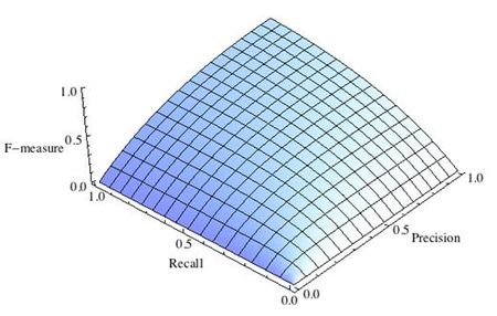
-

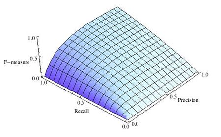
Рис.1 Сбалансированная F-мера,
-

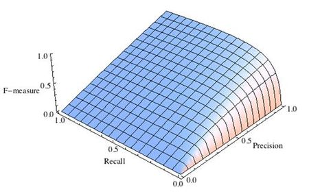
Рис.2 F-мера c приоритетом точности,
-

Рис.3 F-мера c приоритетом полноты,
F-мера достигает максимума при максимальной полноте и точности, и близка к нулю, если один из аргументов близок к нулю.
F-мера является хорошим кандидатом на формальную метрику оценки качества классификатора. Она сводит к одному числу две других основополагающих метрики: точность и полноту. Имея «F-меру» гораздо проще ответить на вопрос: «поменялся алгоритм в лучшую сторону или нет?»
 # код для подсчета метрики F-mera:
 # Пример классификатора, способного проводить различие между всего лишь двумя
 # классами, "пятерка" и "не пятерка" из набора рукописных цифр MNIST
 import numpy as np
 from sklearn.datasets import fetch_openml
 from sklearn.model_selection import cross_val_predict
 from sklearn.linear_model import SGDClassifier
 from sklearn.metrics import f1_score
 mnist = fetch_openml('mnist_784', version=1)
 X, y = mnist["data"], mnist["target"]
 y = y.astype(np.uint8)
 X_train, X_test, y_train, y_test = X[:60000], X[60000:], y[:60000], y[60000:]
 y_train_5 = (y_train == 5) # True для всех пятерок, False для в сех остальных цифр. Задача опознать пятерки
 y_test_5 = (y_test == 5)
 sgd_clf = SGDClassifier(random_state=42) # классификатор на основе метода стохастического градиентного спуска (Stochastic Gradient Descent SGD)
 sgd_clf.fit(X_train, y_train_5) # обучаем классификатор распознавать пятерки на целом обучающем наборе
 y_train_pred = cross_val_predict(sgd_clf, X_train, y_train_5, cv=3)
 print(f1_score(y_train_5, y_train_pred))

 # 0.7325171197343846
ROC-кривая
Кривая рабочих характеристик (англ. Receiver Operating Characteristics curve).
Используется для анализа поведения классификаторов при различных пороговых значениях.
Позволяет рассмотреть все пороговые значения для данного классификатора.
Показывает долю ложно положительных примеров (англ. false positive rate, FPR) в сравнении с долей истинно положительных примеров (англ. true positive rate, TPR).
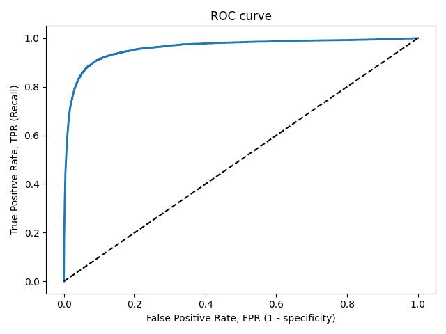
Доля FPR — это пропорция отрицательных образцов, которые были некорректно классифицированы как положительные.
- ,
где TNR — доля истинно отрицательных классификаций (англ. Тrие Negative Rate), представляющая собой пропорцию отрицательных образцов, которые были корректно классифицированы как отрицательные.
Доля TNR также называется специфичностью (англ. specificity). Следовательно, ROC-кривая изображает чувствительность (англ. seпsitivity), т.е. полноту, в сравнении с разностью 1 — specificity.
Прямая линия по диагонали представляет ROC-кривую чисто случайного классификатора. Хороший классификатор держится от указанной линии настолько далеко, насколько это
возможно (стремясь к левому верхнему углу).
Один из способов сравнения классификаторов предусматривает измерение площади под кривой (англ. Area Under the Curve — AUC). Безупречный классификатор будет иметь площадь под ROC-кривой (ROC-AUC), равную 1, тогда как чисто случайный классификатор — площадь 0.5.
 # Код отрисовки ROC-кривой
 # На примере классификатора, способного проводить различие между всего лишь двумя классами
 # "пятерка" и "не пятерка" из набора рукописных цифр MNIST
 from sklearn.metrics import roc_curve
 import matplotlib.pyplot as plt
 import numpy as np
 from sklearn.datasets import fetch_openml
 from sklearn.model_selection import cross_val_predict
 from sklearn.linear_model import SGDClassifier
 mnist = fetch_openml('mnist_784', version=1)
 X, y = mnist["data"], mnist["target"]
 y = y.astype(np.uint8)
 X_train, X_test, y_train, y_test = X[:60000], X[60000:], y[:60000], y[60000:]
 y_train_5 = (y_train == 5)  # True для всех пятерок, False для в сех остальных цифр. Задача опознать пятерки
 y_test_5 = (y_test == 5)
 sgd_clf = SGDClassifier(random_state=42) # классификатор на основе метода стохастического градиентного спуска (Stochastic Gradient Descent SGD)
 sgd_clf.fit(X_train, y_train_5) # обучаем классификатор распозновать пятерки на целом обучающем наборе
 y_train_pred = cross_val_predict(sgd_clf, X_train, y_train_5, cv=3)
 y_scores = cross_val_predict(sgd_clf, X_train, y_train_5, cv=3, method="decision_function")
 fpr, tpr, thresholds = roc_curve(y_train_5, y_scores)
 def plot_roc_curve(fpr, tpr, label=None):
     plt.plot(fpr, tpr, linewidth=2, label=label)
     plt.plot([0, 1], [0, 1], 'k--') # dashed diagonal
     plt.xlabel('False Positive Rate, FPR (1 - specificity)')
     plt.ylabel('True Positive Rate, TPR (Recall)')
     plt.title('ROC curve')
     plt.savefig("ROC.png")
 plot_roc_curve(fpr, tpr)
 plt.show()
Precison-recall кривая
Чувствительность к соотношению классов.
Рассмотрим задачу выделения математических статей из множества научных статей. Допустим, что всего имеется 1.000.100 статей, из которых лишь 100 относятся к математике. Если нам удастся построить алгоритм , идеально решающий задачу, то его TPR будет равен единице, а FPR — нулю. Рассмотрим теперь плохой алгоритм, дающий положительный ответ на 95 математических и 50.000 нематематических статьях. Такой алгоритм совершенно бесполезен, но при этом имеет TPR = 0.95 и FPR = 0.05, что крайне близко к показателям идеального алгоритма.
Таким образом, если положительный класс существенно меньше по размеру, то AUC-ROC может давать неадекватную оценку качества работы алгоритма, поскольку измеряет долю неверно принятых объектов относительно общего числа отрицательных. Так, алгоритм , помещающий 100 релевантных документов на позиции с 50.001-й по 50.101-ю, будет иметь AUC-ROC 0.95.
Precison-recall (PR) кривая. Избавиться от указанной проблемы с несбалансированными классами можно, перейдя от ROC-кривой к PR-кривой. Она определяется аналогично ROC-кривой, только по осям откладываются не FPR и TPR, а полнота (по оси абсцисс) и точность (по оси ординат). Критерием качества семейства алгоритмов выступает площадь под PR-кривой (англ. Area Under the Curve — AUC-PR)
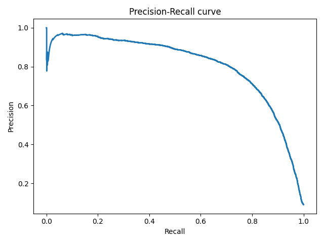
 # Код отрисовки Precison-recall кривой
 # На примере классификатора, способного проводить различие между всего лишь двумя классами
 # "пятерка" и "не пятерка" из набора рукописных цифр MNIST
 from sklearn.metrics import precision_recall_curve
 import matplotlib.pyplot as plt
 import numpy as np
 from sklearn.datasets import fetch_openml
 from sklearn.model_selection import cross_val_predict
 from sklearn.linear_model import SGDClassifier
 mnist = fetch_openml('mnist_784', version=1)
 X, y = mnist["data"], mnist["target"]
 y = y.astype(np.uint8)
 X_train, X_test, y_train, y_test = X[:60000], X[60000:], y[:60000], y[60000:]
 y_train_5 = (y_train == 5) # True для всех пятерок, False для в сех остальных цифр. Задача опознать пятерки
 y_test_5 = (y_test == 5)
 sgd_clf = SGDClassifier(random_state=42) # классификатор на основе метода стохастического градиентного спуска (Stochastic Gradient Descent SGD)
 sgd_clf.fit(X_train, y_train_5) # обучаем классификатор распозновать пятерки на целом обучающем наборе
 y_train_pred = cross_val_predict(sgd_clf, X_train, y_train_5, cv=3)
 y_scores = cross_val_predict(sgd_clf, X_train, y_train_5, cv=3, method="decision_function")
 precisions, recalls, thresholds = precision_recall_curve(y_train_5, y_scores)
 def plot_precision_recall_vs_threshold(precisions, recalls, thresholds):
     plt.plot(recalls, precisions, linewidth=2)
     plt.xlabel('Recall')
     plt.ylabel('Precision')
     plt.title('Precision-Recall curve')
     plt.savefig("Precision_Recall_curve.png")
 plot_precision_recall_vs_threshold(precisions, recalls, thresholds)
 plt.show()
Оценки качества регрессии
Наиболее типичными мерами качества в задачах регрессии являются
Средняя квадратичная ошибка (англ. Mean Squared Error, MSE)
MSE применяется в ситуациях, когда нам надо подчеркнуть большие ошибки и выбрать модель, которая дает меньше больших ошибок прогноза. Грубые ошибки становятся заметнее за счет того, что ошибку прогноза мы возводим в квадрат. И модель, которая дает нам меньшее значение среднеквадратической ошибки, можно сказать, что что у этой модели меньше грубых ошибок.
- и
Cредняя абсолютная ошибка (англ. Mean Absolute Error, MAE)
Среднеквадратичный функционал сильнее штрафует за большие отклонения по сравнению со среднеабсолютным, и поэтому более чувствителен к выбросам. При использовании любого из этих двух функционалов может быть полезно проанализировать, какие объекты вносят наибольший вклад в общую ошибку — не исключено, что на этих объектах была допущена ошибка при вычислении признаков или целевой величины.
Среднеквадратичная ошибка подходит для сравнения двух моделей или для контроля качества во время обучения, но не позволяет сделать выводов о том, на сколько хорошо данная модель решает задачу. Например, MSE = 10 является очень плохим показателем, если целевая переменная принимает значения от 0 до 1, и очень хорошим, если целевая переменная лежит в интервале (10000, 100000). В таких ситуациях вместо среднеквадратичной ошибки полезно использовать коэффициент детерминации —
Коэффициент детерминации
Коэффициент детерминации измеряет долю дисперсии, объясненную моделью, в общей дисперсии целевой переменной. Фактически, данная мера качества — это нормированная среднеквадратичная ошибка. Если она близка к единице, то модель хорошо объясняет данные, если же она близка к нулю, то прогнозы сопоставимы по качеству с константным предсказанием.
Средняя абсолютная процентная ошибка (англ. Mean Absolute Percentage Error, MAPE)
Это коэффициент, не имеющий размерности, с очень простой интерпретацией. Его можно измерять в долях или процентах. Если у вас получилось, например, что MAPE=11.4%, то это говорит о том, что ошибка составила 11,4% от фактических значений.
Основная проблема данной ошибки — нестабильность.
Корень из средней квадратичной ошибки (англ. Root Mean Squared Error, RMSE)
Примерно такая же проблема, как и в MAPE: так как каждое отклонение возводится в квадрат, любое небольшое отклонение может значительно повлиять на показатель ошибки. Стоит отметить, что существует также ошибка MSE, из которой RMSE как раз и получается путем извлечения корня.
Cимметричная MAPE (англ. Symmetric MAPE, SMAPE)
Средняя абсолютная масштабированная ошибка (англ. Mean absolute scaled error, MASE)
MASE является очень хорошим вариантом для расчета точности, так как сама ошибка не зависит от масштабов данных и является симметричной: то есть положительные и отрицательные отклонения от факта рассматриваются в равной степени.
Обратите внимание, что в MASE мы имеем дело с двумя суммами: та, что в числителе, соответствует тестовой выборке, та, что в знаменателе — обучающей. Вторая фактически представляет собой среднюю абсолютную ошибку прогноза. Она же соответствует среднему абсолютному отклонению ряда в первых разностях. Эта величина, по сути, показывает, насколько обучающая выборка предсказуема. Она может быть равна нулю только в том случае, когда все значения в обучающей выборке равны друг другу, что соответствует отсутствию каких-либо изменений в ряде данных, ситуации на практике почти невозможной. Кроме того, если ряд имеет тенденцию к росту либо снижению, его первые разности будут колебаться около некоторого фиксированного уровня. В результате этого по разным рядам с разной структурой, знаменатели будут более-менее сопоставимыми. Всё это, конечно же, является очевидными плюсами MASE, так как позволяет складывать разные значения по разным рядам и получать несмещённые оценки.
Недостаток MASE в том, что её тяжело интерпретировать. Например, MASE=1.21 ни о чём, по сути, не говорит. Это просто означает, что ошибка прогноза оказалась в 1.21 раза выше среднего абсолютного отклонения ряда в первых разностях, и ничего более.
Кросс-валидация
Хороший способ оценки модели предусматривает применение кросс-валидации (cкользящего контроля или перекрестной проверки).
В этом случае фиксируется некоторое множество разбиений исходной выборки на две подвыборки: обучающую и контрольную. Для каждого разбиения выполняется настройка алгоритма по обучающей подвыборке, затем оценивается его средняя ошибка на объектах контрольной подвыборки. Оценкой скользящего контроля называется средняя по всем разбиениям величина ошибки на контрольных подвыборках.
Примечания
- [1] Лекция «Оценивание качества» на www.coursera.org
- [2] Лекция на www.stepik.org о кросвалидации
- [3] Лекция на www.stepik.org о метриках качества, Precison и Recall
- [4] Лекция на www.stepik.org о метриках качества, F-мера
- [5] Лекция на www.stepik.org о метриках качества, примеры
См. также
- Оценка качества в задаче кластеризации
- Кросс-валидация
Источники информации
- [6] Соколов Е.А. Лекция линейная регрессия
- [7] — Дьяконов А. Функции ошибки / функционалы качества
- [8] — Оценка качества прогнозных моделей
- [9] — HeinzBr Ошибка прогнозирования: виды, формулы, примеры
- [10] — egor_labintcev Метрики в задачах машинного обучения
- [11] — grossu Методы оценки качества прогноза
- [12] — К.В.Воронцов, Классификация
- [13] — К.В.Воронцов, Скользящий контроль
Среднеквадратичная ошибка (Mean Squared Error) – Среднее арифметическое (Mean) квадратов разностей между предсказанными и реальными значениями Модели (Model) Машинного обучения (ML):

Рассчитывается с помощью формулы, которая будет пояснена в примере ниже:
$$MSE = frac{1}{n} × sum_{i=1}^n (y_i — widetilde{y}_i)^2$$
$$MSEspace{}{–}space{Среднеквадратическая}space{ошибка,}$$
$$nspace{}{–}space{количество}space{наблюдений,}$$
$$y_ispace{}{–}space{фактическая}space{координата}space{наблюдения,}$$
$$widetilde{y}_ispace{}{–}space{предсказанная}space{координата}space{наблюдения,}$$
MSE практически никогда не равен нулю, и происходит это из-за элемента случайности в данных или неучитывания Оценочной функцией (Estimator) всех факторов, которые могли бы улучшить предсказательную способность.
Пример. Исследуем линейную регрессию, изображенную на графике выше, и установим величину среднеквадратической Ошибки (Error). Фактические координаты точек-Наблюдений (Observation) выглядят следующим образом:

Мы имеем дело с Линейной регрессией (Linear Regression), потому уравнение, предсказывающее положение записей, можно представить с помощью формулы:
$$y = M * x + b$$
$$yspace{–}space{значение}space{координаты}space{оси}space{y,}$$
$$Mspace{–}space{уклон}space{прямой}$$
$$xspace{–}space{значение}space{координаты}space{оси}space{x,}$$
$$bspace{–}space{смещение}space{прямой}space{относительно}space{начала}space{координат}$$
Параметры M и b уравнения нам, к счастью, известны в данном обучающем примере, и потому уравнение выглядит следующим образом:
$$y = 0,5252 * x + 17,306$$
Зная координаты реальных записей и уравнение линейной регрессии, мы можем восстановить полные координаты предсказанных наблюдений, обозначенных серыми точками на графике выше. Простой подстановкой значения координаты x в уравнение мы рассчитаем значение координаты ỹ:

Рассчитаем квадрат разницы между Y и Ỹ:

Сумма таких квадратов равна 4 445. Осталось только разделить это число на количество наблюдений (9):
$$MSE = frac{1}{9} × 4445 = 493$$
Само по себе число в такой ситуации становится показательным, когда Дата-сайентист (Data Scientist) предпринимает попытки улучшить предсказательную способность модели и сравнивает MSE каждой итерации, выбирая такое уравнение, что сгенерирует наименьшую погрешность в предсказаниях.
MSE и Scikit-learn
Среднеквадратическую ошибку можно вычислить с помощью SkLearn. Для начала импортируем функцию:
import sklearn
from sklearn.metrics import mean_squared_error
Инициализируем крошечные списки, содержащие реальные и предсказанные координаты y:
y_true = [5, 41, 70, 77, 134, 68, 138, 101, 131]
y_pred = [23, 35, 55, 90, 93, 103, 118, 121, 129]
Инициируем функцию mean_squared_error(), которая рассчитает MSE тем же способом, что и формула выше:
mean_squared_error(y_true, y_pred)
Интересно, что конечный результат на 3 отличается от расчетов с помощью Apple Numbers:
496.0Ноутбук, не требующий дополнительной настройки на момент написания статьи, можно скачать здесь.
Автор оригинальной статьи: @mmoshikoo
Фото: @tobyelliott
In statistics, the mean squared error (MSE) of an estimator is one of many ways to quantify the difference between values implied by a kernel density estimator and the true values of the quantity being estimated. MSE is a risk function, corresponding to the expected value of the squared error loss or quadratic loss. MSE measures the average of the squares of the «errors.» The error is the amount by which the value implied by the estimator differs from the quantity to be estimated. The difference occurs because of randomness or because the estimator doesn’t account for information that could produce a more accurate estimate.[1]
The MSE is the second moment (about the origin) of the error, and thus incorporates both the variance of the estimator and its bias. For an unbiased estimator, the MSE is the variance. Like the variance, MSE has the same units of measurement as the square of the quantity being estimated. In an analogy to standard deviation, taking the square root of MSE yields the root mean square error or root mean square deviation (RMSE or RMSD), which has the same units as the quantity being estimated; for an unbiased estimator, the RMSE is the square root of the variance, known as the standard deviation.
Contents
- 1 Definition and basic properties
- 1.1 Alternative usages
- 2 Examples
- 3 Interpretation
- 4 Applications
- 5 As a loss function
- 6 See also
- 7 Notes
Definition and basic properties
The MSE of an estimator  with respect to the estimated parameter θ is defined as
![operatorname{MSE}(hat{theta})=operatorname{E}big[(hat{theta}-theta)^2big].](https://en-academic.com/dic.nsf/enwiki/5/495f30ac586e91558efc63561cde0434.png)
The MSE is equal to the sum of the variance and the squared bias of the estimator

The MSE thus assesses the quality of an estimator in terms of its variation and unbiasedness. Note that the MSE is not equivalent to the expected value of the absolute error.
Since MSE is an expectation, it is not a random variable. It may be a function of the unknown parameter θ, but it does not depend on any random quantities. However, when MSE is computed for a particular estimator of θ the true value of which is not known, it will be subject to estimation error. In a Bayesian sense, this means that there are cases in which it may be treated as a random variable.
Alternative usages
In regression analysis, the term mean squared error is sometimes used to refer to the estimate of error variance: residual sum of squares divided by the number of degrees of freedom. This is an observed quantity given a particular sample (and hence is sample-dependent), whereas the definition above is a function of the parameters of the probability distribution of an unknown parameter. For more details, see errors and residuals in statistics.
Also in regression analysis, «mean squared error», often referred to as «out-of-sample mean squared error», can refer to the mean value of the squared deviations of the predictions from the true values, over an out-of-sample test space, generated by a model estimated over a particular sample space. This also is an observed quantity, and it varies by sample and by out-of-sample test space.
Examples
Suppose we have a random sample of size n from a population,  . The usual estimator for the mean is the sample average
which has an expected value of μ (so it is unbiased) and a mean square error of

For a Gaussian distribution this is the best unbiased estimator (that is, it has the lowest MSE among all unbiased estimators), but not, say, for a uniform distribution.
The usual estimator for the variance is

This is unbiased (its expected value is σ2), and its MSE is[2]

where μ4 is the fourth central moment of the distribution or population and γ2 = μ4 / σ4 − 3 is the excess kurtosis.
However, one can use other estimators for σ2 which are proportional to  , and an appropriate choice can always give a lower mean square error. If we define

then the MSE is
![begin{align}
operatorname{MSE}(S^2_a)&=operatorname{E}left(left(frac{n-1}{a} S^2_{n-1}-sigma^2right)^2 right) \
&=frac{n-1}{n a^2}[(n-1)gamma_2+n^2+n]sigma^4-frac{2(n-1)}{a}sigma^4+sigma^4
end{align}](https://en-academic.com/dic.nsf/enwiki/9/f49ce44866b736ae4989b3d192b7d41f.png)
This is minimized when

For a Gaussian distribution, where γ2 = 0, this means the MSE is minimized when dividing the sum by a = n + 1, whereas for a Bernoulli distribution with p = 1/2 (a coin flip), γ2 = − 2, the MSE is minimized for a = n − 1 + 2 / n. (Note that this particular case of the Bernoulli distribution has the lowest possible excess kurtosis; this can be proved by Jensen’s inequality as follows. The fourth central moment is an upper bound for the square of variance, so that the least value for their ratio is one, therefore, the least value for the excess kurtosis is -2, achieved, for instance, by a Bernoulli with p=1/2.) So no matter what the kurtosis, we get a «better» estimate (in the sense of having a lower MSE) by scaling down the unbiased estimator a little bit. Even among unbiased estimators, if the distribution is not Gaussian the best (minimum mean square error) estimator of the variance may not be 
The following table gives several estimators of the true parameters of the population, μ and σ2, for the Gaussian case.[3]
| True value | Estimator | Mean squared error |
|---|---|---|
| θ = μ | = the unbiased estimator of the population mean,  |
 |
| θ = σ2 | = the unbiased estimator of the population variance,  |
 |
| θ = σ2 | = the biased estimator of the population variance,  |
 |
| θ = σ2 | = the biased estimator of the population variance,  |
 |
Note that:
- The MSEs shown for the variance estimators assume i.i.d. so that . The result for follows easily from the variance that is 2n − 2.
- Unbiased estimators may not produce estimates with the smallest total variation (as measured by MSE): the MSE of is larger than that of or .
- Estimators with the smallest total variation may produce biased estimates: typically underestimates σ2 by
 i.i.d. so that
  . The result for
  variance that is
  or
or  .
.
Interpretation
An MSE of zero, meaning that the estimator predicts observations of the parameter θ with perfect accuracy, is the ideal, but is practically never possible.
Values of MSE may be used for comparative purposes. Two or more statistical models may be compared using their MSEs as a measure of how well they explain a given set of observations: The unbiased model with the smallest MSE is generally interpreted as best explaining the variability in the observations and is called the best unbiased estimator or MVUE (Minimum Variance Unbiased Estimator).
Both linear regression techniques such as analysis of variance estimate the MSE as part of the analysis and use the estimated MSE to determine the statistical significance of the factors or predictors under study. The goal of experimental design is to construct experiments in such a way that when the observations are analyzed, the MSE is close to zero relative to the magnitude of at least one of the estimated treatment effects.
MSE is also used in several stepwise regression techniques as part of the determination as to how many predictors from a candidate set to include in a model for a given set of observations.
Applications
- Minimizing MSE is a key criterion in selecting estimators:see Minimum mean-square error. Among unbiased estimators, the minimal MSE is equivalent to minimizing the variance, and is obtained by the MVUE. However, a biased estimator may have lower MSE; see estimator bias.
- In statistical modelling the MSE, representing the difference between the actual observations and the response predicted by the model, is used to determine whether the model does not fit the data or whether the model can be simplified by removing terms.
As a loss function
Squared error loss is one of the most widely used loss functions in statistics, though its widespread use stems more from mathematical convenience than considerations of actual loss in applications. Carl Friedrich Gauss, who introduced the use of mean squared error, was aware of its arbitrariness and was in agreement with objections to it on these grounds.[1] The mathematical benefits of mean squared error are particularly evident in its use at analyzing the performance of linear regression, as it allows one to partition the variation in a dataset into variation explained by the model and variation explained by randomness.
- Criticism
The use of mean squared error without question has been criticized by the decision theorist James Berger. Mean squared error is the negative of the expected value of one specific utility function, the quadratic utility function, which may not be the appropriate utility function to use under a given set of circumstances. There are, however, some scenarios where mean squared error can serve as a good approximation to a loss function occurring naturally in an application.[4]
Like variance, mean squared error has the disadvantage of heavily weighting outliers.[5] This is a result of the squaring of each term, which effectively weights large errors more heavily than small ones. This property, undesirable in many applications, has led researchers to use alternatives such as the mean absolute error, or those based on the median.
See also
- Mean squared prediction error
- Mean square weighted deviation
- Mean percentage error
- Squared deviations
- Peak signal-to-noise ratio
- Root mean square deviation
Notes
- ^ a b Lehmann, E. L.; Casella, George (1998). Theory of Point Estimation (2nd ed.). New York: Springer. ISBN 0-387-98502-6. MR1639875.
- ^ Mood, A.; Graybill, F.; Boes, D. (1974). Introduction to the Theory of Statistics (3rd ed.). McGraw-Hill. p. 229.
- ^ DeGroot, Morris H. (1980). Probability and Statistics (2nd ed.). Addison-Wesley.
- ^ Berger, James O. (1985). «2.4.2 Certain Standard Loss Functions». Statistical decision theory and Bayesian Analysis (2nd ed.). New York: Springer-Verlag. p. 60. ISBN 0-387-96098-8. MR0804611.
- ^ Sergio Bermejo, Joan Cabestany (2001) «Oriented principal component analysis for large margin classifiers», Neural Networks, 14 (10), 1447–1461.
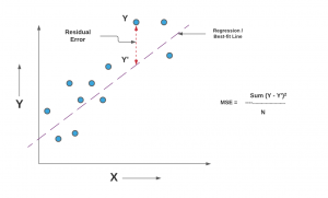
In this post, you will learn about the concepts of the mean-squared error (MSE) and R-squared, the difference between them, and which one to use when evaluating the linear regression models. You also learn Python examples to understand the concepts in a better manner
What is Mean Squared Error (MSE)?
The Mean squared error (MSE) represents the error of the estimator or predictive model created based on the given set of observations in the sample. Intuitively, the MSE is used to measure the quality of the model based on the predictions made on the entire training dataset vis-a-vis the true label/output value. In other words, it can be used to represent the cost associated with the predictions or the loss incurred in the predictions. And, the squared loss (difference between true & predicted value) is advantageous because they exaggerate the difference between the true value and the predicted value. Two or more regression models created using a given sample of data can be compared based on their MSE. The lesser the MSE, the better the regression model is. When the linear regression model is trained using a given set of observations, the model with the least mean sum of squares error (MSE) is selected as the best model. The Python or R packages select the best-fit model as the model with the lowest MSE or lowest RMSE when training the linear regression models.
In 1805, the French mathematician Adrien-Marie Legendre, who first published the sum of squares method for gauging the quality of the model stated that squaring the error before summing all of the errors to find the total loss is convenient. The question that may be asked is why not calculate the error as the absolute value of loss (difference between y and y_hat in the following formula) and sum up all the errors to find the total loss. The absolute value of error is not convenient, because it doesn’t have a continuous derivative, which does not make the function smooth. And, the functions that are not smooth are difficult to work with when trying to find closed-form solutions to the optimization problems by employing linear algebra concepts.
Mathematically, the MSE can be calculated as the average sum of the squared difference between the actual value and the predicted or estimated value represented by the regression model (line or plane). It is also termed as mean squared deviation (MSD). This is how it is represented mathematically:
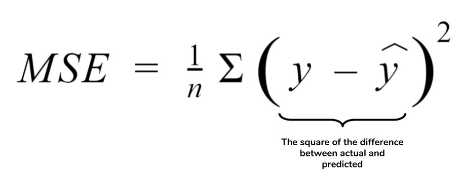
The value of MSE is always positive. A value close to zero will represent better quality of the estimator/predictor (regression model).
An MSE of zero (0) represents the fact that the predictor is a perfect predictor.
When you take a square root of MSE value, it becomes root mean squared error (RMSE). RMSE has also been termed root mean square deviation (RMSD). In the above equation, Y represents the actual value and the Y_hat represents the predicted value that could be found on the regression line or plane. Here is the diagrammatic representation of MSE for a simple linear or univariate regression model:
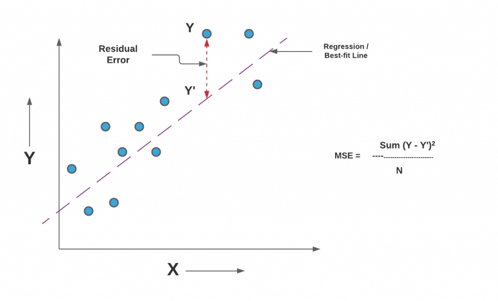
What is R-Squared?
R-Squared is the ratio of the sum of squares regression (SSR) and the sum of squares total (SST). Sum of Squares Regression (SSR) represents the total variation of all the predicted values found on the regression line or plane from the mean value of all the values of response variables. The sum of squares total (SST) represents the total variation of actual values from the mean value of all the values of response variables. R-squared value is used to measure the goodness of fit or best-fit line. The greater the value of R-Squared, the better is the regression model as most of the variation of actual values from the mean value get explained by the regression model. However, we need to take caution while relying on R-squared to assess the performance of the regression model. This is where the adjusted R-squared concept comes into the picture. This would be discussed in one of the later posts. R-Squared is also termed as the coefficient of determination. For the training dataset, the value of R-squared is bounded between 0 and 1, but it can become negative for the test dataset if the SSE is greater than SST. Greater the value of R-squared would also mean a smaller value of MSE. If the value of R-Squared becomes 1 (ideal world scenario), the model fits the data perfectly with a corresponding MSE = 0. As the value of R-squared increases and become close to 1, the value of MSE becomes close to 0.
Here is a visual representation to understand the concepts of R-Squared in a better manner.
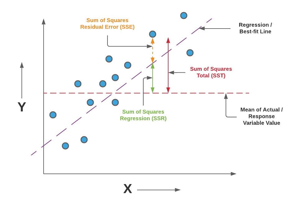
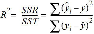
Pay attention to the diagram and note that the greater the value of SSR, the more is the variance covered by the regression / best fit line out of total variance (SST). R-Squared can also be represented using the following formula:
R-Squared = 1 – (SSE/SST)
Pay attention to the diagram and note that the smaller the value of SSE, the smaller is the value of (SSE/SST), and hence greater will be the value of R-Squared. Read further details on R-squared in this blog – R-squared/R2 in linear regression: Concepts, Examples
R-Squared can also be expressed as a function of mean squared error (MSE). The following equation represents the same. You may notice that as MSE increases, the value of R2 will decrease owing to the fact that the ratio of MSE and Var(y) will increase resulting in the decrease in the value of R2.
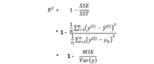
Difference between Mean Square Error & R-Squared
The similarity between mean-squared error and R-Squared is that they both are a type of metrics that are used for evaluating the performance of the linear regression models.
The difference is that MSE gets pronounced based on whether the data is scaled or not. For example, if the response variable is housing price in the multiple of 10K, MSE will be different (lower) than when the response variable such as housing pricing is not scaled (actual values). This is where R-Squared comes to the rescue. R-Squared is also termed the standardized version of MSE. R-squared represents the fraction of variance of the actual value of the response variable captured by the regression model rather than the MSE which captures the residual error.
MSE or R-Squared – Which one to Use?
It is recommended to use R-Squared or rather adjusted R-Squared for evaluating the model performance of the regression models. This is primarily because R-Squared captures the fraction of variance of actual values captured by the regression model and tends to give a better picture of the quality of the regression model. Also, MSE values differ based on whether the values of the response variable are scaled or not. A better measure instead of MSE is the root mean squared error (RMSE) which takes care of the fact related to whether the values of the response variable are scaled or not.
One can alternatively use MSE or R-Squared based on what is appropriate and the need of the hour. However, the disadvantage of using MSE than R-squared is that it will be difficult to gauge the performance of the model using MSE as the value of MSE can vary from 0 to any larger number. However, in the case of R-squared, the value is bounded between 0 and 1. A value of R-squared closer to 1 would mean that the regression model covers most part of the variance of the values of the response variable and can be termed as a good model. However, with the MSE value, depending on the scale of values of the response variable, the value will be different and hence, it would be difficult to assess for certain whether the regression model is good or otherwise.
MSE or R-Squared Python Code Example
Here is the python code representing how to calculate mean squared error or R-Squared value while working with regression models. Pay attention to some of the following in the code given below:
- Sklearn.metrics mean_squared_error and r2_score is used for measuring the MSE and R-Squared values. Input to this methods are actual values and predicted values.
- Sklearn Boston housing dataset is used for training a multiple linear regression model using Sklearn.linear_model LinearRegression
import pandas as pd
from sklearn.model_selection import train_test_split
from sklearn.preprocessing import StandardScaler
from sklearn.linear_model import LinearRegression
from sklearn.pipeline import make_pipeline
from sklearn.metrics import mean_squared_error, r2_score
from sklearn import datasets
#
# Load the Sklearn Boston Dataset
#
boston_ds = datasets.load_boston()
X = boston_ds.data
y = boston_ds.target
#
# Create a training and test split
#
X_train, X_test, y_train, y_test = train_test_split(X, y, test_size=0.3, random_state=42)
#
# Fit a pipeline using Training dataset and related labels
#
pipeline = make_pipeline(StandardScaler(), LinearRegression())
pipeline.fit(X_train, y_train)
#
# Calculate the predicted value for training and test dataset
#
y_train_pred = pipeline.predict(X_train)
y_test_pred = pipeline.predict(X_test)
#
# Mean Squared Error
#
print('MSE train: %.3f, test: %.3f' % (mean_squared_error(y_train, y_train_pred),
                mean_squared_error(y_test, y_test_pred)))
#
# R-Squared
#
print('R^2 train: %.3f, test: %.3f' % (r2_score(y_train, y_train_pred),
                r2_score(y_test, y_test_pred)))
Conclusions
Here is the summary of what you learned in this post regarding mean square error (MSE) and R-Squared and which one to use?
- MSE represents the residual error which is nothing but sum of squared difference between actual values and the predicted / estimated values divided by total number of records.
- R-Squared represents the fraction of variance captured by the regression model.
- The disadvantage of using MSE is that the value of MSE varies based on whether the values of response variable is scaled or not. If scaled, MSE will be lower than the unscaled values.
- Author
- Recent Posts

I have been recently working in the area of Data analytics including Data Science and Machine Learning / Deep Learning. I am also passionate about different technologies including programming languages such as Java/JEE, Javascript, Python, R, Julia, etc, and technologies such as Blockchain, mobile computing, cloud-native technologies, application security, cloud computing platforms, big data, etc. For latest updates and blogs, follow us on Twitter. I would love to connect with you on Linkedin.
Check out my latest book titled as First Principles Thinking: Building winning products using first principles thinking

Ajitesh Kumar
I have been recently working in the area of Data analytics including Data Science and Machine Learning / Deep Learning. I am also passionate about different technologies including programming languages such as Java/JEE, Javascript, Python, R, Julia, etc, and technologies such as Blockchain, mobile computing, cloud-native technologies, application security, cloud computing platforms, big data, etc. For latest updates and blogs, follow us on Twitter. I would love to connect with you on Linkedin.
Check out my latest book titled as First Principles Thinking: Building winning products using first principles thinking