From Wikipedia, the free encyclopedia
In statistics the mean squared prediction error or mean squared error of the predictions of a smoothing or curve fitting procedure is the expected value of the squared difference between the fitted values implied by the predictive function  and the values of the (unobservable) function g. It is an inverse measure of the explanatory power of
  and can be used in the process of cross-validation of an estimated model.
If the smoothing or fitting procedure has projection matrix (i.e., hat matrix) L, which maps the observed values vector  to predicted values vector
  via
via  then
then
![operatorname {MSPE}(L)=operatorname {E}left[left(g(x_{i})-widehat {g}(x_{i})right)^{2}right].](https://wikimedia.org/api/rest_v1/media/math/render/svg/123e8c977dc8ed61b5af45da081253556a293acb)
The MSPE can be decomposed into two terms: the mean of squared biases of the fitted values and the mean of variances of the fitted values:
![{displaystyle ncdot operatorname {MSPE} (L)=sum _{i=1}^{n}left(operatorname {E} left[{widehat {g}}(x_{i})right]-g(x_{i})right)^{2}+sum _{i=1}^{n}operatorname {var} left[{widehat {g}}(x_{i})right].}](https://wikimedia.org/api/rest_v1/media/math/render/svg/c2f2e662ed164b7a590da8b7a2112f880f617d0e)
Knowledge of g is required in order to calculate the MSPE exactly; otherwise, it can be estimated.
Computation of MSPE over out-of-sample data[edit]
The mean squared prediction error can be computed exactly in two contexts. First, with a data sample of length n, the data analyst may run the regression over only q of the data points (with q < n), holding back the other n – q data points with the specific purpose of using them to compute the estimated model’s MSPE out of sample (i.e., not using data that were used in the model estimation process). Since the regression process is tailored to the q in-sample points, normally the in-sample MSPE will be smaller than the out-of-sample one computed over the n – q held-back points. If the increase in the MSPE out of sample compared to in sample is relatively slight, that results in the model being viewed favorably. And if two models are to be compared, the one with the lower MSPE over the n – q out-of-sample data points is viewed more favorably, regardless of the models’ relative in-sample performances. The out-of-sample MSPE in this context is exact for the out-of-sample data points that it was computed over, but is merely an estimate of the model’s MSPE for the mostly unobserved population from which the data were drawn.
Second, as time goes on more data may become available to the data analyst, and then the MSPE can be computed over these new data.
Estimation of MSPE over the population[edit]
When the model has been estimated over all available data with none held back, the MSPE of the model over the entire population of mostly unobserved data can be estimated as follows.
For the model  where
where  , one may write
![{displaystyle ncdot operatorname {MSPE} (L)=g^{text{T}}(I-L)^{text{T}}(I-L)g+sigma ^{2}operatorname {tr} left[L^{text{T}}Lright].}](https://wikimedia.org/api/rest_v1/media/math/render/svg/afa4a2de4f014dc1c2cf31bc803f5d642c68a26f)
Using in-sample data values, the first term on the right side is equivalent to
![{displaystyle sum _{i=1}^{n}left(operatorname {E} left[g(x_{i})-{widehat {g}}(x_{i})right]right)^{2}=operatorname {E} left[sum _{i=1}^{n}left(y_{i}-{widehat {g}}(x_{i})right)^{2}right]-sigma ^{2}operatorname {tr} left[left(I-Lright)^{T}left(I-Lright)right].}](https://wikimedia.org/api/rest_v1/media/math/render/svg/e9f60fa601829826d71a7d40c74ee73564dfab9c)
Thus,
![{displaystyle ncdot operatorname {MSPE} (L)=operatorname {E} left[sum _{i=1}^{n}left(y_{i}-{widehat {g}}(x_{i})right)^{2}right]-sigma ^{2}left(n-operatorname {tr} left[Lright]right).}](https://wikimedia.org/api/rest_v1/media/math/render/svg/b6da6d150e8f3f19e291b2e7fd536f366690eff3)
If  is known or well-estimated by
  , it becomes possible to estimate MSPE by
![{displaystyle ncdot operatorname {widehat {MSPE}} (L)=sum _{i=1}^{n}left(y_{i}-{widehat {g}}(x_{i})right)^{2}-{widehat {sigma }}^{2}left(n-operatorname {tr} left[Lright]right).}](https://wikimedia.org/api/rest_v1/media/math/render/svg/d4890e1a2ff444ff87af3a9a80dfd00ee733f1bf)
Colin Mallows advocated this method in the construction of his model selection statistic Cp, which is a normalized version of the estimated MSPE:

where p the number of estimated parameters p and is computed from the version of the model that includes all possible regressors.
That concludes this proof.
See also[edit]
- Mean squared error
- Errors and residuals in statistics
- Law of total variance
Further reading[edit]
- Pindyck, Robert S.; Rubinfeld, Daniel L. (1991). «Forecasting with Time-Series Models». Econometric Models & Economic Forecasts (3rd ed.). New York: McGraw-Hill. pp. 516–535. ISBN 0-07-050098-3.
The SPE chart values exceeding the control limits are related to observations that do not behave in the same way as the ones used to create the model (in-control data), in the sense that there is a breakage of the correlation structure of the model.
From: Comprehensive Chemometrics, 2009
Intelligent optimal setting control of the cobalt removal process
Chunhua Yang, Bei Sun, in Modeling, Optimization, and Control of Zinc Hydrometallurgical Purification Process, 2021
7.3.1 Data-driven online operating state monitoring
Data-driven online process monitoring is an approach to detect the type of current operating state. Multivariate statistical process monitoring (MSPM) is a widely applied data-driven online process monitoring method [11–14]. It recognizes the type of current operating state by observing the underlying mode of process variables [15].
In ACP, the process variables, including output states, inlet conditions, and reaction conditions, are highly correlated. Variation of the process variables is driven by some underlying events, e.g., change of raw materials and manipulated variables, maintenance, etc. [11]. These underlying events give rise to the change of working conditions, which can be reflected by the variation of process variables. The MSPM method detects the mode change of process variables by using multivariate statistical projection (MSP) methods [16]. These methods project the correlated raw process variables to a latent variable space. The latent variables are linearly uncorrelated, have lower dimension, and can be used to detect the operating state.
Principal component analysis (PCA) is a typical latent variable extraction method in process monitoring [17–19]. Denote x∈Rm as the data sample including m process variables. If there exist N data samples representing the normal operating state, then a sample set containing the characteristic information of the normal operating state can be constructed as
X=[x1x2…xN]T∈RN×m,
where each row represents a data sample xiT.
The performance of PCA will be affected if the scales of the raw process variables are different. Therefore, the data sample set X is first scaled to zero mean and unit variance. The scaled data sample set is (X−μ)/Dδ. μ=[μ1μ2…μm] and Dδ=[δ1δ2…δm] are the mean value and standard deviation of the original data sample set, respectively. The covariance matrix of X is approximated by Σ=XTX/(N−1). The eigenvalues of the covariance matrix Λ=diag[ν1ν2…νm], νi−1⩾νi⩾0(i=2,3,…,m). Its orthogonal eigenvector is p=[p1p2…pm], which satisfies Σ=pΛpT. If ∑i=1nkνi/∑i=1mνi>ην(1⩽nk⩽m), where ην is a predefined contribution threshold of latent variables or principal components and nk is the number of retained principal components, then X can be projected on the principal component subspace and the residual subspace as
(7.23)X=pT+E,
where p is the principal loadings and T=pTX is the scores of nk latent variables. The residual vector is therefore
(7.24)E=X−TpT=(1−ppT)X.
After the construction of the PCA model, some statistical indices indicating the current operating state can be obtained, e.g., the Hotelling T2 and squared prediction error (SPE) metrics [20]. Here, T2 represents the deviation between the current operating state and the normal operating state and SPE is the residual or squared distance of the current observation from the model plane [11]:
(7.25)T2=xnewTpΛ−1pTxnew,
(7.26)SPE=‖Enew‖2=‖(1−ppT)xnew‖2.
In the building of the PCA model, only the data samples under the normal operating state are utilized. If the T2 and SPE values of the current operating state exceed the upper limits [18], then it is regarded as an abnormal operating state. The upper limits of T2 and SPE are [21]
(7.27)T2⩽τ2,τ2=nk(N2−1)N(N−nk)Fnk,N−1,α,
(7.28)SPE⩽γ2,γ2=θ1(cα2θ2h02θ1+1+θ2h0(h0−1)θ12)1/nk,
where Fnk,N−1,α is an F distribution with nk and N−nk degrees of freedom for a given significance level α, θi=∑j=k+1mλji(i=1,2,3), h0=1−(2θ1θ3)/(3θ22), and cα is the normal deviate corresponding to the upper (1−α) percentile.
In order to evaluate the detection performance of T2 and SPE, the PCA model and the upper limits of T2 and SPE are obtained using 100 data samples under the normal operating state. A number of 50 other data samples were used for testing. The test results are shown in Figs. 7.8 and 7.9. Samples exceeding the upper limits of T2 and SPE are considered as abnormal operating states. It can be observed from the test result that:

Figure 7.8. T2 of test sample.

Figure 7.9. SPE of test sample.
- (i)
-
Samples detected as abnormal operating states have larger modeling errors.
- (ii)
-
SPE mainly reflects the stochastic disturbance forced on the process; it has a more intense distribution and clear variation trajectory than T2; and
- (iii)
-
T2 mainly reflects the variation of the essential process dynamics.
Read full chapter
URL:
https://www.sciencedirect.com/science/article/pii/B9780128195925000181
Volume 4
T. Kourti, in Comprehensive Chemometrics, 2009
4.02.3.5 Fault Diagnosis and Contribution Plots
In classical quality control where only quality variables are monitored, it is up to process operators and engineers to try to diagnose an assignable cause for an out-of-control signal, using their process knowledge and a one-at-a-time inspection of process variables. When PLS or PCA models are used to construct the multivariate control charts, they provide the user with the tools to diagnose assignable causes. Diagnostic or contribution plots can be extracted from the underlying PLS or PCA model at the point where an event has been detected. The plot reveals the group of process variables making the greatest contributions to the deviations in SPEx and the scores. Although these plots will not unequivocally diagnose the cause, they provide an insight into possible causes and thereby greatly narrow the search.
4.02.3.5.1 Contributions to SPE
When an out-of-control situation is detected on the SPE plot, the contribution of each variable of the original data set is simply given by (xnew,j−xˆnew,j)2. Variables with high contributions are investigated.
4.02.3.5.2 Contributions to Hotelling’s T2
Contributions to an out-of-limits value in the Hotelling’s T2-chart are obtained as follows: A bar plot of the normalized scores (ti/sti)2 is plotted and scores with high normalized values are further investigated by calculating variable contributions. A variable contribution plot indicates how each variable involved in the calculation of that score contributes to it. The contribution of each variable of the original data set to the score of component q is given by
(29)cj=pq,j(xj−x―j)forPCAandcj=wq,j(xj−x―j)forPLS
where cj is the contribution of the jth variable at the given observation, pq,j is the loading and wq,j is the weight of this variable to the score of the PC q, and x―j is its mean value (which is 0 for mean-centered data).4 Variables on this plot that appear to have the largest contributions to it, but also the same sign as the score should be investigated (contributions of the opposite sign will only make the score smaller).
When there are K scores with high values, an ‘overall average contribution’ per variable is calculated, over all the K scores, as shown below:
- Step 1:
-
Repeat for all the K high scores (K ≤ A)
- •
-
Calculate the contribution of a variable xj to the normalized score (ti/sti)2:
conti,j=tisti2pi,j(xj−x―j)
- •
-
Set contribution equal to 0 if it is negative (i.e., sign opposite of sign of score)
- Step 2:
-
Calculate the total contribution of variable xj: xj:CONTj=∑i=1K(conti,j)
- Step 3:
-
Investigate variables with high contributions
The variable contribution plots provide a powerful tool for fault identification. However, the user should be careful with its interpretation. In general, this approach will point to a variable or a group of variables that contribute numerically to the out-of-control signal; these variables and any variables highly correlated with them should be investigated to assign causes. The role of the contribution plots to fault isolation is to indicate which of the variables are related to the fault rather than to reveal the actual cause of it. Sometimes, the cause of a fault is not a measured variable. The variables with high contributions to the contribution plots are simply the signature of such faults. Reactor fouling and reaction impurities are two characteristic examples of complex process faults where they manifest themselves on other measured variables.1,4
Read full chapter
URL:
https://www.sciencedirect.com/science/article/pii/B9780444527011000132
Speech Synthesis Based on Linear Prediction
Bishnu S. Atal, in Encyclopedia of Physical Science and Technology (Third Edition), 2003
III.B Determination of Predictor Coefficients
Let us discuss now the method of determining the predictor coefficients for a given speech segment. The predictor coefficients that minimize the mean-squared prediction error Ep are obtained by setting the partial derivative of the error with respect to each ak equal to zero. The error as a function of the predictor coefficients is given by
(7)Ep=1N∑n=1Nsn−∑k=1paksn−k2.
We set the partial derivatives ∂Ep/∂ ak equal to zero:
(8)∂Ep∂ak=0,k=1,2,…,p.
This gives p simultaneous equations in p unknowns:
(9)∑k=1pakϕik=ci,k=1,2,…,p,
where
φik=∑n=1Ns(n−i)s(n−k)
and
(10)ci=∑n=1Nsnsn−i.
(10) can be expressed in matrix notations as
(11)Φa=c,
where the element in the ith row and kth column of p × p matrix Φ is ϕik, ak is the kth element of the p-dimensional vector a, and ci is the ith element of the p-dimensional vector c. The unknown predictor coefficients can be determined by solving the p simultaneous equations given inEq. (9) or the matrix equation given inEq. (11).
We have not yet discussed an important question—what is the correct value of p? As we mentioned earlier, each resonance adds two additional predictor coefficients to the prediction. In speech there are approximately four or five resonances and it would be necessary to set p = 10. But we must also add a few extra coefficients for the excitation produced by the vocal cords, the coupling of the nasal tract, and the sound radiation from lips. This suggests that p = 12 is a reasonable estimate of the prediction order. Figure 10 shows a plot of the root mean squared (rms) prediction error as a function of prediction order p for both voiced and unvoiced speech. It is clear that not much has to be gained by selecting a value of p much greater than 12.

FIGURE 10. Normalized root mean squared (rms) prediction error plotted against p, the prediction order, for voiced and unvoiced speech.
Read full chapter
URL:
https://www.sciencedirect.com/science/article/pii/B0122274105007201
Disease Modelling and Public Health, Part B
J. Sunil Rao, Jie Fan, in Handbook of Statistics, 2017
4 Predicting Community Characteristics for Colon Cancer Patients From the Florida Cancer Data System
We next analyzed colon cancer cases in a statewide registry breaking up our sample into a training and testing sample. Our goal was to predict community characteristics for a set of test sample individuals as characterized by their census tract community information.
The Florida Cancer Data System (FCDS) is the Florida statewide cancer registry (https://fcds.med.miami.edu/). It began data collection in 1981 and in 1994, became part of the National Program of Cancer Registries (NPCR) which is under the administration of the Centers for Disease Control (CDC). Two hundred and thirty hospitals report approximated 115,000 unduplicated newly diagnosed cases per year. Currently, FCDS contains over 3,000,000 cancer incidence records.
Specifically at the time of analysis, there were 3,116,030 observations of 144 variables in the original FCDS data set. There were 353,407 observations left after filtering for colon cancer and 314,633 observations left after filtering invalid survival dates. Further filtering to remove curious coding on tumor size, sex, grade, race, smoking status, treatment type, node positivity, radiation treatment, and chemotherapy information, left 45,917 observations for analysis.
There were 2890 census tracts in the filtered data. We kept the census tracts with number of observations no smaller than 25, which left us with 18,732 observations among 466 census tracts. We focused our attention to Miami-Dade county which left 210 census tracts for our analysis. We randomly chose 100 census tracts and 25 observations from each tract as our training data for the linking model. The response variable of interest was the square of age.
The coefficients of the variables in the linking model are in Table 6. We removed variables that had small t-values relative to the large sample size of the dataset (Miller, 2002). The variables that remained in the linking model were race, log survival time, sex, number of positive nodes, smoking history, radiation, and chemotherapy.
Table 6. Linking Model Fit
| Term | Estimate | t-Value | 95% CI |
|---|---|---|---|
| Intercept | 6539.51 | 54.59 | [6304.71, 6744.33] |
| Log. surv | −42.22 | −6.74 | [−54.51, −29.94] |
| Race | −1003.04 | −23.98 | [−1085.03, −921.05] |
| Sex | 162.21 | 7.37 | [119.08, 205.34] |
| Tumor grade | 83.33 | 4.03 | [42.84, 123.84] |
| Tumor size | −0.74 | −2.21 | [−1.41, −0.09] |
| Number of positive nodes | −23.87 | −6.58 | [−30.99, −16.76] |
| Smoking | −297.50 | −13.41 | [−340.98, −254.03] |
| Surgery | 215.03 | 2.59 | [52.09, 377.97] |
| Radiation | −436.05 | −8.89 | [−532.24, −339.87] |
| Chemo | −953.94 | −31.58 | [−1013.14, −894.74] |
For test data, we chose 10 observations (or all the observations in a tract, whichever is smaller), from each of 842 Miami-Dade tracts with no data lost to variable filtering (33 tracts were left out due to variable filtering issues). This left a total test set sample size of 7266 observations. Our predictive geocoding analysis focused around census tracts in the Miami-Dade area. We focused on four community variables: health insurance coverage status (estimated percent uninsured based on the total noninstitutionalized population), employment status (estimated unemployment rate for people 16 years of age and older), median income in the past 12 months in 2013 inflation-adjusted dollars (based on households), and educational attainment (estimated as a percent of total who did not graduate high school). These were extracted from the 2009 to 2015 5-Year American Community Survey (ACS) (2014) (https://www.census.gov/data/developers/updates/acs-5-yr-summary-available-2009-2013.html).
Table 7 shows the predictive performance with respect to characterizing community characteristics for test samples using the different predictors: the CMPI using REML estimation, CMPI using the OBP estimate of Jiang et al. (2015), CMPI based on modeling the spatial correlation structure across census tracts (see Section 2.4), prediction to a random chosen census tract and simply using the community variable population mean in each census tract. We report the empirical mean squared prediction error (MSPE) averaged across all census tracts as well as its various components (the squared bias and the variance). We also report the variance of the predicted values across census tracts (BT) and the variance of the true community variable values across census tracts (TBT).
Table 7. Comparison of Methods With Respect to Predictive Performance
| Method | MSPE | Bias2 | Variance | BT Variance | TBT Variance |
|---|---|---|---|---|---|
| CMPI (REML)—education | 364.22 | 212.27 | 154.34 | 102.47 | 195.32 |
| CMPI (REML)—income | 1078.92 | 895.07 | 186.85 | 162.76 | 569.80 |
| CMPI (REML)—unemployed | 51.4 | 35.11 | 16.63 | 10.92 | 34.50 |
| CMPI (REML)—uninsured | 223.01 | 163.73 | 60.18 | 41.82 | 131.66 |
| CMPI (OBP)—education | 366.79 | 209.58 | 159.66 | 87.90 | |
| CMPI (OBP)—income | 1057.50 | 890.47 | 169.68 | 135.60 | |
| CMPI (OBP)—unemployed | 47.99 | 35.24 | 12.95 | 7.22 | |
| CMPI (OBP)—uninsured | 231.67 | 146.97 | 86.01 | 56.45 | |
| CMPI (SP)—education | 360.56 | 220.81 | 141.95 | 105.56 | |
| CMPI (SP)—income | 1089.89 | 903.20 | 189.71 | 154.92 | |
| CMPI (SP)—unemployed | 51.59 | 35.86 | 15.98 | 12.55 | |
| CMPI (SP)—uninsured | 222.50 | 161.87 | 61.54 | 42.02 | |
| Random—education | 434.67 | 205.71 | 232.55 | 232.60 | |
| Random—income | 1048.16 | 677.63 | 376.61 | 370.66 | |
| Random—unemployed | 64.39 | 35.03 | 29.81 | 29.86 | |
| Random—uninsured | 251.30 | 145.12 | 107.88 | 107.07 | |
| Population mean—education | 202.09 | 201.09 | 1.01 | 0 | |
| Population mean—income | 680.03 | 677.89 | 2.17 | 0 | |
| Population mean—unemployed | 35.17 | 35.11 | 0.05 | 0 | |
| Population mean—uninsured | 143.87 | 143.62 | 0.25 | 0 |
Reported measures are MSPE, squared bias, average within tract variance, between tract (BT) variance, and true between tract (TBT) variance.
Table 7 results are illuminating and can be summarized as follows:
- 1.
-
The CMPI estimators generally significantly outperform the random allocation predictor with respect to MSPE and this is primarily driven by decreased variance in within census tract predictions. This can be attributed to the linking model which borrows strength across tracts amounting to a type of smoothing (and hence variance reduction) for specific tract predictions.
- 2.
-
The naive population mean predictor actually does very well with respect to MSPE because there is no variance associated with these predictions within tract.
- 3.
-
Incorporating spatial structure into the CMPI predictor can result in gains in reduced MSPE. But this appears to be only true for the education and uninsured community variables, and the gains are small.
- 4.
-
Robust estimation using the OBP can produce gains in MSPE but the results are not uniform across all the community variables. Median income and percent unemployed seem to benefit while percent education and percent uninsured do not.
- 5.
-
Simply focusing on within tract summaries reveals an incomplete picture since by those measures alone, the best predictions would come from the most naive population mean estimator. However, this estimator will assign the same value for all individuals across all census tracts. Clearly this is overly naive since now between tract variability will be captured. When examining empirical between tract variance estimates, it is clear that this naive estimator significantly underestimates true tract-to-tract variance. The CMPI estimators fare much better but do still underestimate between tract variances. This is due to the model fit which captures relatively little of this variance as estimated by the random effect variance component.
Fig. 3 shows the community variable predictive performance as oriented across census tracts in Miami-Dade. Green coloring indicates highly accurate predictions and as the color shading becomes darker blue, the accuracy of the predictions worsen (as measured by MPSE). Overall, predictions seem to be quite accurate.

Fig. 3. MSPE map for Miami-Dade county—unclustered.
4.1 Clustering of Census Tracts Adds Robustness to Predictions
The next set of analyses examined predictive performance of the various estimators while allowing for clustering of census tracts with respect to community variables. The logic here is that even if an individual is incorrectly classified to a given tract, as long as the true tract is similar to the predicted one, then it would still be considered an accurate prediction. In order to allow this robustness to be at play, we clustered census tracts according to the four community variables.
Fig. 4 shows the gap statistic analysis (Tibshirani et al., 2001) using the union of the 466 tracts with at least 25 observations after variable filtering and the 875 tracts in the Miami-Dade area. The gap statistic indicated that three clusters are a reasonable estimate of the true number of “community clusters.” Table 8 gives the resulting means of the four community variables by cluster and the number of tracts in each cluster.

Fig. 4. Gap statistic plot showing number of “community clusters” based on four community variables.
Table 8. Community Variable Means by Community Cluster
| Cluster Number | Education | Median Income | Unemployed | Uninsured | Number of Tracts |
|---|---|---|---|---|---|
| 1 | 9.87 | 47.18 | 11.25 | 20.98 | 581 |
| 2 | 11.74 | 92.20 | 7.50 | 11.32 | 184 |
| 3 | 32.47 | 34.49 | 15.11 | 29.49 | 366 |
Table 9 shows how predictive performance is affected allowing for community clustering. We report only one CMPI estimator (the REML). It is quite clear that clustering improves MSPE performance for all estimators but the relative gains when comparing CMPI to random and population mean estimators increase with clustering. Similar patterns to Table 7 are observed when looking at within tract summaries vs between tract summary measures.
Table 9. Comparison of Methods With Respect to Predictive Performance With Clustering
| Method | MSPE | Bias2 | Variance | BT Variance | TBT Variance |
|---|---|---|---|---|---|
| CMPI (REML)—education | 297.24 | 202.81 | 95.94 | 59.90 | 195.32 |
| CMPI (REML)—income | 993.95 | 696.13 | 302.25 | 230.78 | 569.80 |
| CMPI (REML)—unemployed | 40.75 | 35.41 | 5.42 | 4.36 | 34.50 |
| CMPI (REML)—uninsured | 171.56 | 141.95 | 30.06 | 24.32 | 131.66 |
| Random—education | 307.84 | 203.33 | 106.15 | 106.03 | |
| Random—income | 1301.13 | 688.30 | 622.33 | 624.31 | |
| Random—unemployed | 44.98 | 35.28 | 9.84 | 9.87 | |
| Random—uninsured | 204.92 | 149.47 | 56.31 | 56.46 | |
| Population mean—education | 202.07 | 200.91 | 1.17 | 0 | |
| Population mean—income | 687.83 | 684.82 | 3.05 | 0 | |
| Population mean—unemployed | 35.37 | 35.27 | 0.10 | 0 | |
| Population mean—uninsured | 143.33 | 143.04 | 0.28 | 0 |
Reported measures are MSPE, squared bias, average within tract variance, between tract (BT) variance, and true between tract (TBT) variance.
Fig. 5 shows the MSPE spatial plots for Miami-Dade based on community clustering. Now, internal quantiles are fixed from the unclustered analysis so as to be able to compare Figs. 2 and 3 properly. Specifically, the 25th, 50th, and 75th percentiles are fixed at the unclustered values. Now, if more green appears, it indicates that clustering is improving MSPE as compared to the unclustered analysis. Fig. 5 shows that indeed this is the case. Much more green is produced. In conclusion, community clustering adds robustness to the predictive geocoding analysis.

Fig. 5. MSPE map for Miami-Dade county—clustered.
Read full chapter
URL:
https://www.sciencedirect.com/science/article/pii/S0169716117300251
Multiple Regression
Gary Smith, in Essential Statistics, Regression, and Econometrics (Second Edition), 2015
The Coefficient of Determination, R2
As with the simple regression model, the model’s predictive accuracy can be gauged by the coefficient of determination, R2, which compares the sum of squared prediction errors to the sum of squared deviations of Y about its mean:
(10.9)R2=∑i=1n(yi−yˆ)2∑i=1n(yi−y¯)2
In our consumption model, R2 = 0.999, indicating that our multiple regression model explains an impressive 99.9 percent of the variation in the annual consumption. The multiple correlation coefficient R is the square root of R2.
Read full chapter
URL:
https://www.sciencedirect.com/science/article/pii/B9780128034590000108
Volume 3
F. Arteaga, A.J. Ferrer-Riquelme, in Comprehensive Chemometrics, 2009
3.06.3.2.5 Minimization of the squared prediction error method
Given a new individual, z, its scores vector is τ=PTz. The new observation can be reconstructed as zˆ=Pτ=P(PTz), so that e=z−zˆ=z−(PPT)z=(IK−PPT)z is the residual (prediction error). Note that matrix (IK−PPT) is idempotent and symmetric. From this, it follows that the sum of the squared prediction error (SPE) can be expressed as SPEz=eTe=zT(IK−PPT)z. The SPE can be expressed in blocks, as a function of z# (unknown) and z* (known), and a reasonable estimation criterion would be to choose z#, so that the SSE is minimized for the new observation, z. Wise and Ricker36 adopt the same approach and Arteaga and Ferrer3 prove that minimizing the SPE as a function of z#, and substituting the result into the expression τˆ=PTzˆ=P#Tzˆ#+P*Tz*, it follows that τˆ=(P*TP*)−1P*Tz*. Therefore, like the iterative method, this algorithm is equivalent to the PMP method (Equation (4)).
Although Nelson et al.5 state that, compared to the PMP algorithm, Wise and Ricker’s method is more difficult to implement and does not lend itself readily to error analysis, Arteaga and Ferrer3 show that both algorithms, PMP and SPE, yield the same score vector estimator.
Read full chapter
URL:
https://www.sciencedirect.com/science/article/pii/B9780444527011001253
Statistical Control of Measures and Processes
A.J. Ferrer-Riquelme, in Comprehensive Chemometrics, 2009
1.04.9.2.2 PCA-based MSPC: online process monitoring (Phase II)
Once the reference PCA model and the control limits for the multivariate control charts are obtained, new process observations can be monitored online. When a new observation vector zi is available, after preprocessing it is projected onto the PCA model yielding the scores and the residuals, from which the value of the Hotelling TA2 and the value of the SPE are calculated. This way, the information contained in the original K variables is summarized in these two indices, which are plotted in the corresponding multivariate TA2 and SPE control charts. No matter what the number of the original variables K is, only two points have to be plotted on the charts and checked against the control limits. The SPE chart should be checked first. If the points remain below the control limits in both charts, the process is considered to be in control. If a point is detected to be beyond the limits of one of the charts, then a diagnostic approach to isolate the original variables responsible for the out-of-control signal is needed. In PCA-based MSPC, contribution plots37 are commonly used for this purpose.
Contribution plots can be derived for abnormal points in both charts. If the SPE chart signals a new out-of-control observation, the contribution of each original kth variable to the SPE at this new abnormal observation is given by its corresponding squared residual:
(37)Cont(SPE;xnew,k)=enew,k2=(xnew,k−xnew,k*)2
where enew,k is the residual corresponding to the kth variable in the new observation and xnew,k* is the prediction of the kth variable xnew,k from the PCA model.
In case of using the DModX statistic, the contribution of each original kth variable to the DModX is given by44
(38)Cont(DModX;xnew,k)=wkenew,k
where wk is the square root of the explained sum of squares for the kth variable. Variables with high contributions in this plot should be investigated.
If the abnormal observation is detected by the TA2 chart, the diagnosis procedure is carried out in two steps: (i) a bar plot of the normalized scores for that observation (tnew,a/λa)2 is plotted and the ath score with the highest normalized value is selected; (ii) the contribution of each original kth variable to this ath score at this new abnormal observation is given by
(39)Cont(tnew,a;xnew,k)=pakxnew,k
where pak is the loading of the kth variable at the ath component. A plot of these contributions is created. Variables on this plot with high contributions but with the same sign as the score should be investigated (contributions of the opposite sign will only make the score smaller). When there are some scores with high normalized values, an overall average contribution per variable can be calculated over all the selected scores.39
Contribution plots are a powerful tool for fault diagnosis. They provide a list of process variables that contribute numerically to the out-of-control condition (i.e., they are no longer consistent with NOCs), but they do not reveal the actual cause of the fault. Those variables and any variables highly correlated with them should be investigated. Incorporation of technical process knowledge is crucial to diagnose the problem and discover the root causes of the fault.
Apart from the TA2 and SPE control charts, other charts such as the univariate time-series plots of the scores or scatter score plots can be useful (both in Phase I and II) for detecting and diagnosing out-of-control situations and also for improving process understanding.
Read full chapter
URL:
https://www.sciencedirect.com/science/article/pii/B978044452701100096X
Factor Analysis
Christof Schuster, Ke-Hai Yuan, in Encyclopedia of Social Measurement, 2005
Predicting the Factor Scores
Because the factor model assumes that the variables are determined to a considerable extent by a linear combination of the factors ξi1, …, ξiq, it is often of interest to determine the factor scores for each individual. Two approaches to predicting factor scores from the variable raw scores are discussed here. Both approaches assume variables and factors to be jointly normally distributed.
The so-called regression factor scores are obtained as
ξˆ=ΦΛ′Σ−1x.
It can be shown that this predictor minimizes the average squared prediction error, E{∑j=1q(ξˆj−ξj)2}, among all factor score predictors that are linear combinations of the variables.
The Bartlett factor score predictor is given by
ξˆ=(Λ′Ψ−1Λ)−1Λ′Ψ−1x.
This expression also minimizes the average squared prediction error among all factor score predictors that are linear combinations of the variables. In addition, the Bartlett factor score predictor is conditionally unbiased, that is, E(ξ˜|ξ)=ξ. Notice that when calculating the factor scores, the matrices Λ and Ψ are replaced by their estimates. In these cases, the optimum property under which the predictors have been derived may not apply. The formula for the Bartlett factor scores can be expressed equivalently when Ψ is replaced with Σ. An advantage of this formulation is that the factor scores can be calculated even if Ψ is singular, which may occur if uniquenesses are zero (Heywood case).
The use of factor scores is problematic because the factor loadings and the factor intercorrelations cannot be defined uniquely. The predicted factor scores will depend on the selected rotation procedure; therefore, factor scores resulting from different rotation procedures may rank order individuals differently. In addition, factor scores are problematic to use as independent variables in regression models because their values differ from the true values, which typically leads to bias in the regression coefficients.
Read full chapter
URL:
https://www.sciencedirect.com/science/article/pii/B0123693985001626
Multiple Regression
Andrew F. Siegel, Michael R. Wagner, in Practical Business Statistics (Eighth Edition), 2022
Regression Coefficients and the Regression Equation
The intercept or constant term, a, and the regression coefficients b1, b2, and b3 are found by the computer using the method of least squares. Among all possible regression equations with various values for these coefficients, these are the ones that make the sum of squared prediction errors the smallest possible for these particular magazines. The regression equation, or prediction equation, is
Predicted page costs=a+b1X1+b2X2+b3X3=248,638+10.73(Audience)−1,020(Percentmale)−1.32(Medianincome)
The intercept, a = $248,638, suggests that the typical charge for a one-page color ad in a magazine with no paid subscribers, no men among its readership, and no income among its readers is $248,638. However, there are no such magazines in this data set, so it may be best to view the intercept, a, as a possibly helpful step in getting the best predictions and not interpret it too literally.
Read full chapter
URL:
https://www.sciencedirect.com/science/article/pii/B9780128200254000129
Multiple Regression
Andrew F. Siegel, in Practical Business Statistics (Seventh Edition), 2016
Regression Coefficients and the Regression Equation
The intercept or constant term, a, and the regression coefficients b1, b2, and b3, are found by the computer using the method of least squares. Among all possible regression equations with various values for these coefficients, these are the ones that make the sum of squared prediction errors the smallest possible for these particular magazines. The regression equation, or prediction equation, is
Predictedpagecosts=a+b1X1+b2X2+b3X3=−22,385+10.50658Audience−20,779Percentmale+1.09198Medianincome
The intercept, a = −$22,385, suggests that the typical charge for a one-page color ad in a magazine with no paid subscribers, no men among its readership, and no income among its readers is − $22,385, suggesting that such an ad has negative value. However, there are no such magazines in this data set, so it may be best to view the intercept, a, as a possibly helpful step in getting the best predictions and not interpret it too literally.
Read full chapter
URL:
https://www.sciencedirect.com/science/article/pii/B9780128042502000122
We encounter predictions in everyday life and work: what will be the high temperature tomorrow, what will be the sales of a product, what will be the price of fuel, how large will be the harvest of grain at the end of the season, and so on. Often such predictions come from authoritative sources: the weather bureau, the government, think tanks. These predictions, like those that come from our own statistical models, are likely to be somewhat off target from the actual outcome.
This chapter introduces a simple, standard way to quantify the size of prediction errors: the root mean square prediction error (RMSE). Those five words are perhaps a mouthful, but as you’ll see, “root mean square” is not such a difficult operation.
Prediction error
We often think of “error” as the result of a mistake or blunder. That’s not really the case for prediction error. Prediction models are built using the resources available to us: explanatory variables that can be measured, accessible data about previous events, our limited understanding of the mechanisms at work, and so on. Naturally, given such flaws our predictions will be imperfect. It seems harsh to call these imperfections an “error”. Nonetheless, Prediction error is the name given to the deviation between the output of our models and the way things eventually turned out in the real world.
The use we can make of a prediction depends on how large those errors are likely to be. We have to say “likely to be” because, at the time we make the prediction, we don’t know what the actual result will be. Chapter 5 introduced the idea of a prediction interval: a range of values that we believe the actual result is highly likely to be in. “Highly likely” is conventionally taken to be 95%.
It may seem mysterious how one can anticipate what an error is likely to be, but the strategy is simple. In order to guide our predictions of the future, we look at our records of the past. The data we use to train a statistical model contains the values of the response variable as well as the explanatory variables. This provides the opportunity to assess the performance of the model. First, generate prediction outputs using as inputs the values of the explanatory variables, Then, compare the prediction outputs to the actual value of the response variable.
The comparison process is illustrated in Table 16.1 and, equivalently, Figure 16.1. The error is the numerical difference between the actual response value and the model output. The error is calculated from our data on a row-by-row basis: one error for each row in our data. The error will be positive when the actual response is larger than the model output, negative when the actual response is smaller, and would be zero if the actual response equals the model output.
Table 16.1: Prediction error from a model mpg ~ hp + cyl of automobile fuel economy versus engine horsepower and number of cylinders. The actual response variable, mpg, is compared to the model output to produce the error and square error.
| hp | cyl | mpg | model_output | error | square_error |
|---|---|---|---|---|---|
| 110 | 6 | 21.0 | 20.29 | 0.71 | 0.51 |
| 110 | 6 | 21.0 | 20.29 | 0.71 | 0.51 |
| 93 | 4 | 22.8 | 25.74 | -2.94 | 8.67 |
| 110 | 6 | 21.4 | 20.29 | 1.11 | 1.24 |
| 175 | 8 | 18.7 | 15.56 | 3.14 | 9.85 |
| 105 | 6 | 18.1 | 20.55 | -2.45 | 6.00 |
| … and so on for 32 rows altogether. |
Figure 16.1: A graphical presentation of Table 16.1. The data layer presents the actual values of the input and output variables. The model output is displayed in a statistics layer by a dash. The error is shown in an interval layer. To emphasize that the error can be positive or negative, color is used to show the sign.
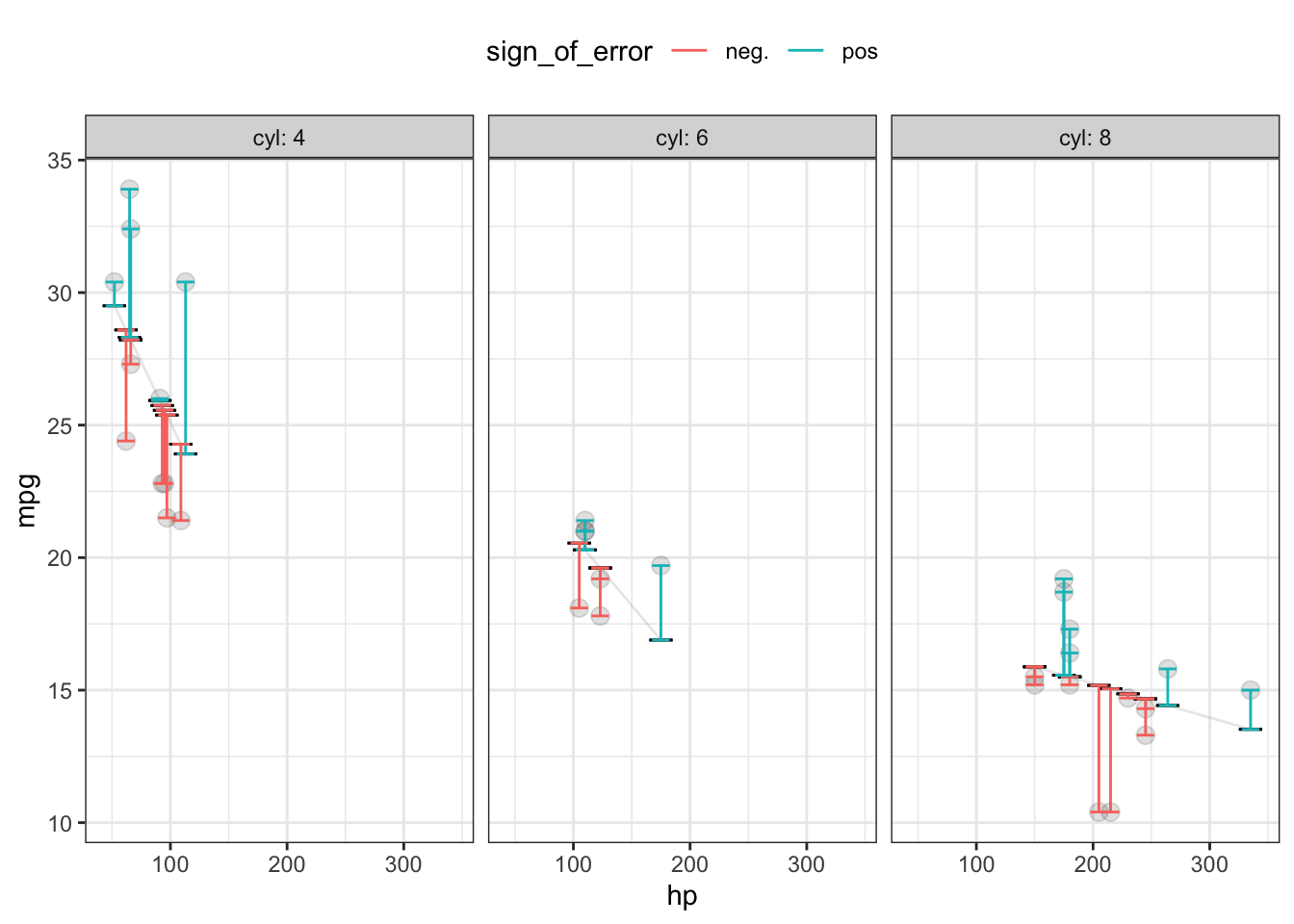
Once each row-by-row error has been found, we consolidate these errors into a single number representing an overall measure of the performance of the model. One easy way to do this is based on the square error, also shown in Table 16.1 and Figure 16.1. The squaring process turns any negative errors into positive square errors.
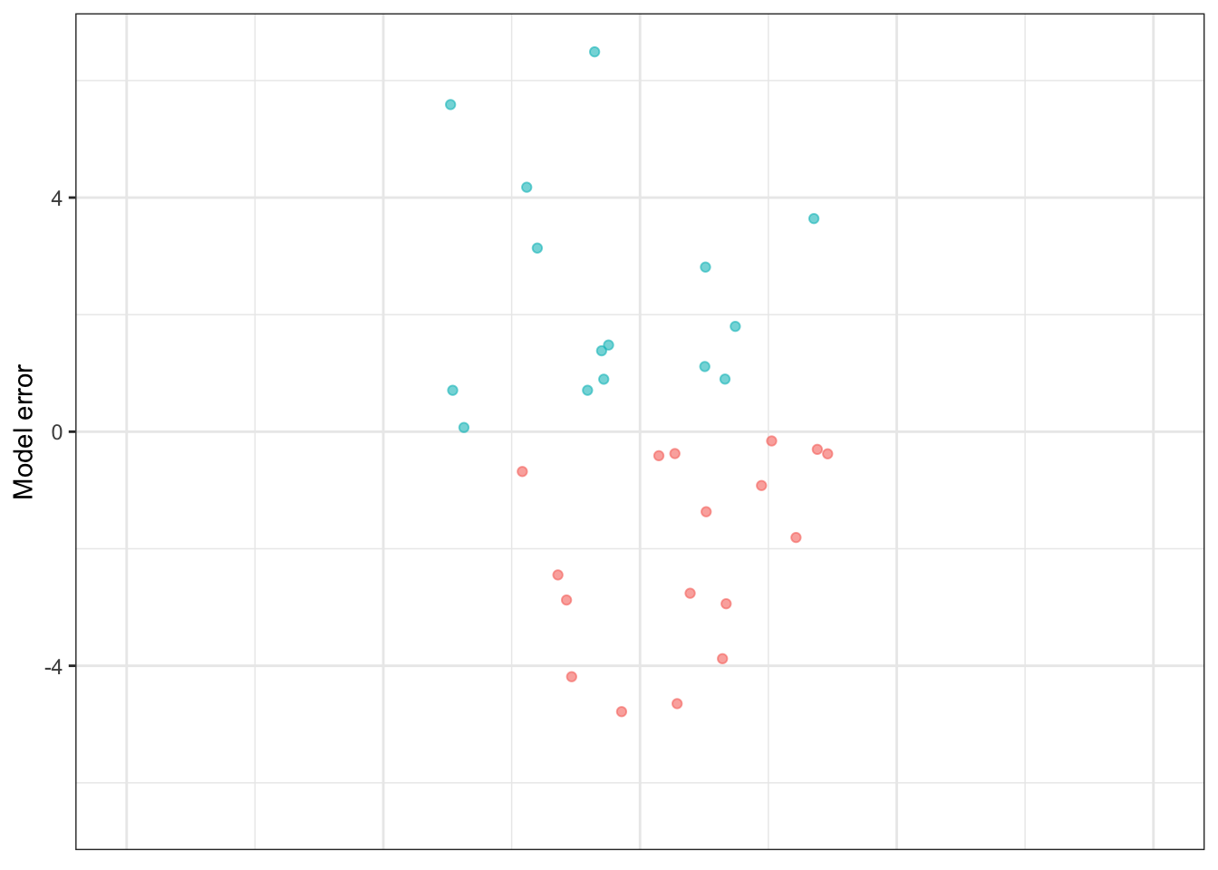
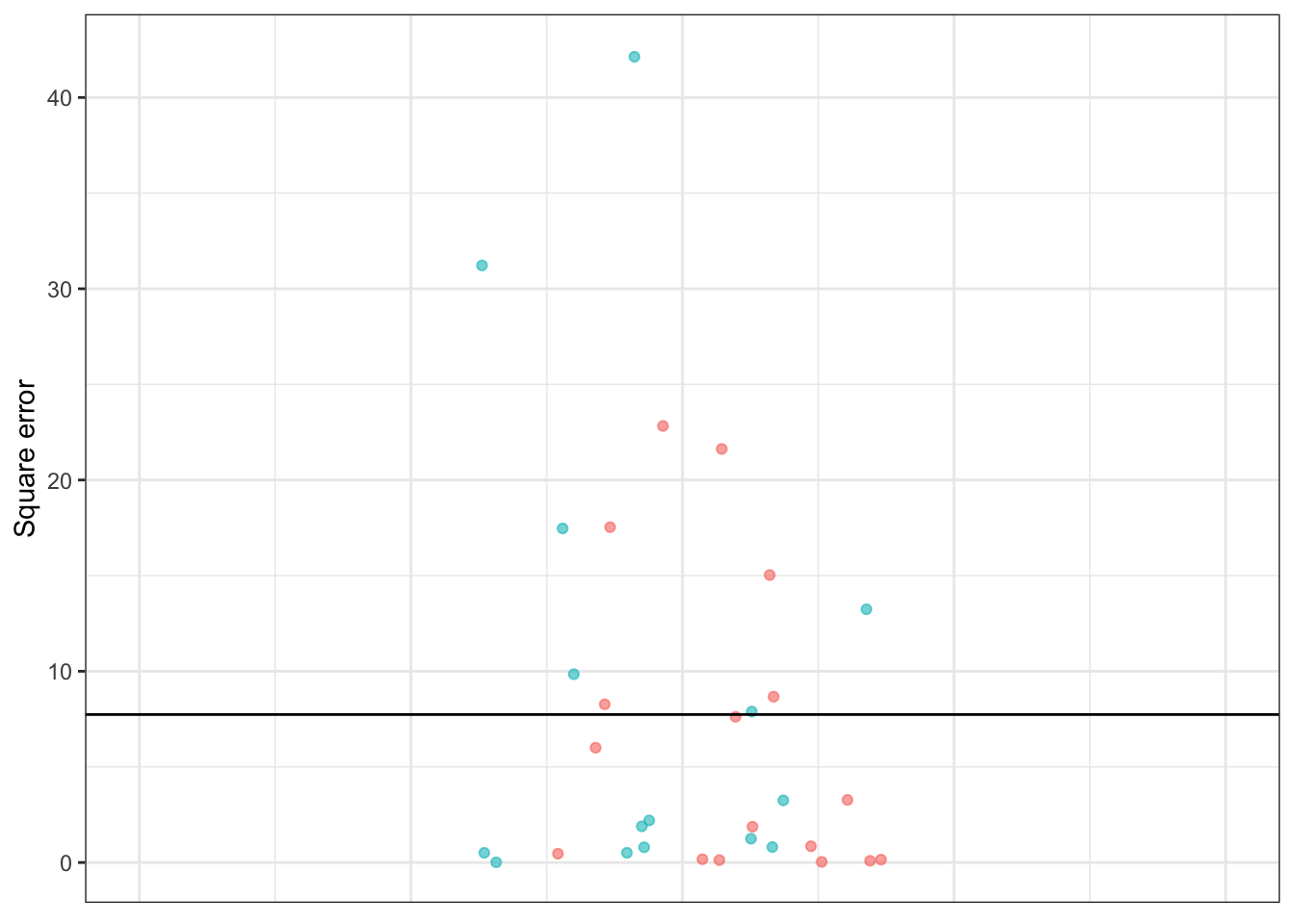
Figure 16.2: The prediction errors and square errors corresponding to Table 16.1 and Figure 16.1. The color shows the sign of the error. Since errors are both positive and negative in sign, overall they are centered on zero. But square errors are always positive, so the mean square error is positive.
Adding up those square errors gives the so-called sum of square errors (SSE). The SSE depends, of course, on both how large the individual errors are and how many rows there are in the data. For Table 16.1, the SSE is
247.61 miles-per-gallon.
The mean square error (MSE) is the average size of the square errors, for example dividing the sum of square errors by the number of rows in the data frame. In Table 16.1, the MSE is simply the SSE divided by the number of rows in the data frame. In Table 16.1 the MSE is 247.61 / 32 = 7.74 square-miles per square-gallon.
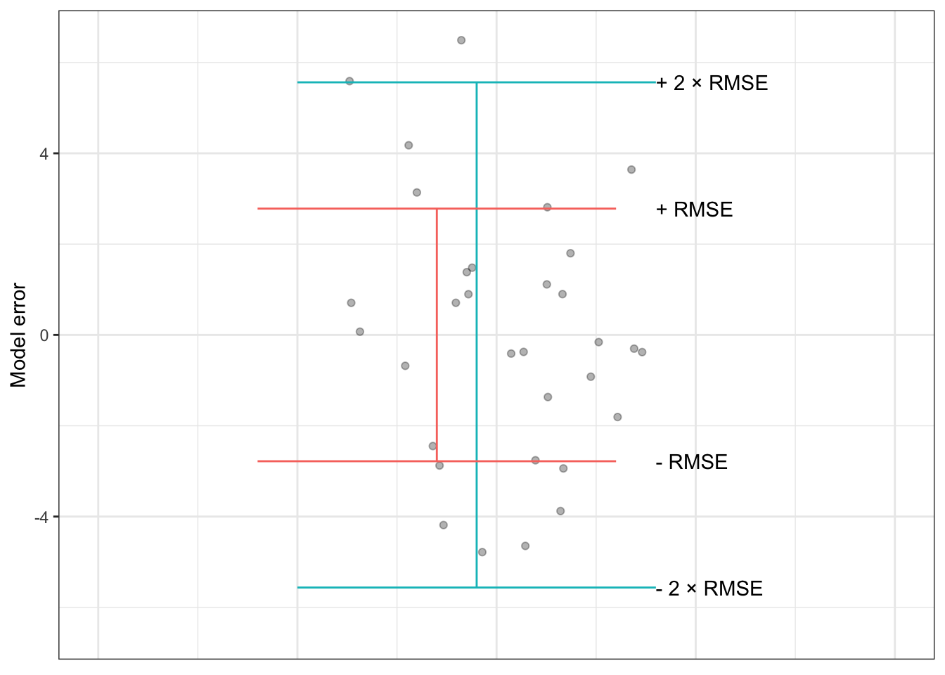
Figure 16.3: The model errors from Table 16.1 shown along with interval ± RMSE and ± 2 × RMSE. The shorter interval encompasses about 67% of the errors, the longer interval covers about 95% of the errors.
Yes, you read that right: square-miles per square-gallon. It’s important to keep track of the physical units of a prediction. These will always be the same as the physical units of the response variable. For instance, in Table 16.1, the response variable is in terms of miles-per-gallon, and so the prediction itself is in miles-per-gallon. Similarly, the prediction error, being the difference between the response value and the predicted value, is in the same units, miles-per-gallon.
Things are a little different for the square error. Squaring a quantity changes the units. For instance, squaring a quantity of 2 meters gives 4 square-meters. This is easy to understand with meters and square-meters; squaring a length produces an area. (This length-to-area conversion is the motivation behind using the word “square.”) For other quantities, such as time, the units are unfamiliar. Square the quantity “15 seconds” and you’ll get 225 square-seconds. Square the quantity “11 chickens” and you’ll get 121 square-chickens. This is not a matter of being silly, but of careful presentation of error.
A mean square error is intended to be a typical size for a square error. But the units, for instance square-miles-per-square-gallon in Table 16.1, can be hard to visualize. For this reason, most people prefer to take the square root of the mean square prediction error. This changes the units back to those of the response variable, e.g. miles-per-gallon, and is yet another way of presenting the magnitude of prediction error.
The root mean square error (RMSE) is simply the square root of the mean square prediction error. For example, in Table 16.1, the RMSE is 2.78 miles-per-gallon, which is just the square root of the MSE of 7.74 square-miles per square-gallon.
Prediction intervals and RMSE
As described in Chapter 5, predictions can be presented as a prediction interval sufficiently long to cover the large majority of the actual outputs. Another way to think about the length of the prediction interval is in terms of the magnitude typical prediction error. In order to contain the majority of actual outputs, the prediction interval ought to reach upwards beyond the typical prediction error and, similarly, reach downwards by the same amount.
The RMSE provides an operational definition of the magnitude of a typical error. So a simple way to construct a prediction interval is to fix the upper end at the prediction function output plus the RMSE and the lower end at the prediction function output minus the RMSE.
It turns out that constructing a prediction interval using ± RMSE provides a roughly 67% interval: about 67% of individual error magnitudes are within ± RMSE of the model output. In order to produce an interval covering roughly 95% of the error magnitudes, the prediction interval is usually calculated using the model output ± 2 × RMSE.
This simple way of constructing prediction intervals is not the whole story. Another component to a prediction interval is “sampling variation” in the model output. Sampling variation will be introduced in Chapter 15.
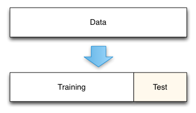
Training and testing data
When you build a prediction model, you have a data frame containing both the response variable and the explanatory variables. This data frame is sometimes called the training data, because the computer uses it to select a particular member from the modeler’s choice of the family of functions for the model, that is, to “train the model.”
In training the model, the computer picks a member of the family of functions that makes the model output as close as possible to the response values in the training data. As described in Chapter 15, if you had used a new and different data frame for training, the selected function would have been somewhat different because it would be tailored to that new data frame.
In making a prediction, you are generally interested in events that you haven’t yet seen. Naturally enough, an event you haven’t yet seen cannot be part of the training data. So the prediction error that we care about is not the prediction error calculated from the training data, but that calculated from new data. Such new data is often called testing data.
Ideally, to get a useful estimate of the size of prediction errors, you should use a testing data set rather than the training data. Of course, it can be very convenient to use the training data for testing. Sometimes no other data is available. Many statistical methods were first developed in an era when data was difficult and expensive to collect and so it was natural to use the training data for testing. A problem with doing this is that the estimated model error will tend to be smaller on the training data than on new data. To compensate for this, as described in Chapter 21, statistical methods used careful accounting, including quantities such as “degrees of freedom,” to compensate mathematically for the underestimation in the error estimate.
Nowadays, when data are plentiful, it’s feasible to split the available data into two parts: a set of rows used for training the model and another set of rows for testing the model. Even better, a method called cross validation effectively lets you use all your data for training and all your data for testing, without underestimating the prediction model’s error. Cross validation is discussed in Chapter 18.
Example: Predicting winning times in hill races
The Scottish hill race data contains four related variables: the race length, the race climb, the sex class, and the winning time in that class. Figures 10.7 and 10.8 in Section ?? show two models of the winning time:
time ~ lengthin Figure 10.7time ~ length + climb + sexin 10.8
Suppose there is a brand-new race trail introduced, with length 20 km, climb 1000 m, and that you want to predict the women’s winning time.
Using these inputs, the prediction function output is
time ~ lengthproduces output 7400 secondstime ~ length + climb + sexproduces output 7250 seconds
It’s to be expected that the two models will produce different predictions; they take different input variables.
Which of the two models is better? One indication is the size of the typical prediction error for each model. To calculate this, we use some of the data as “testing data” as in Tables 16.2 and 16.3. With the testing data (as with the training data) we already know the actual winning time of the race, so calculating the row-by-row errors and square errors for each model is easy.
Table 16.2: time ~ distance: Testing data and the model output and errors from the time ~ distance model. The mean square error is 1,861,269, giving a root mean square error of 1364 seconds.
| distance | climb | sex | time | model_output | error | square_error |
|---|---|---|---|---|---|---|
| 20.0 | 1180 | M | 7616 | 7410 | 206 | 42,436 |
| 20.0 | 1180 | W | 9290 | 7410 | 1880 | 3,534,400 |
| 19.3 | 700 | M | 4974 | 7143 | -2169 | 4,704,561 |
| 19.3 | 700 | W | 5749 | 7143 | -1394 | 1,943,236 |
| 21.0 | 520 | M | 5299 | 7791 | -2492 | 6,210,064 |
| 21.0 | 520 | W | 6101 | 7791 | -1690 | 2,856,100 |
| … and so on for 46 rows altogether. |
Table 16.3: time ~ distance + climb + sex: Testing data and the model output and errors from the time ~ distance + climb + sex model. The mean square error is 483,073 square seconds, giving a root mean square error of 695 seconds.
| distance | climb | sex | time | model_output | error | square_error |
|---|---|---|---|---|---|---|
| 20.0 | 1180 | M | 7616 | 6422 | 1194 | 1,425,636 |
| 20.0 | 1180 | W | 9290 | 7856 | 1434 | 2,056,356 |
| 19.3 | 700 | M | 4974 | 5360 | -386 | 148,996 |
| 19.3 | 700 | W | 5749 | 6525 | -776 | 602,176 |
| 21.0 | 520 | M | 5299 | 5341 | -42 | 1,764 |
| 21.0 | 520 | W | 6101 | 6488 | -387 | 149,769 |
| … and so on for 46 rows altogether. |
Using the testing data, we find that the root mean square error is
time ~ lengthhas RMSE 1364 secondstime ~ length + climb + sexhas RMSE 695 seconds
Clearly, the time ~ length + climb + sex model produces better predictions than the simpler time ~ length model.
The race is run. The women’s winning time turns out to be 8034 sec. Were the predictions right?
Obviously both predictions, 7250 and 7400 secs, were off. You would hardly expect such simple models to capture all the relevant aspects of the race (the weather? the trail surface? whether the climb is gradual throughout or particularly steep in one place? the abilities of other competitors). So it’s not a question of the prediction being right on target but of how far off the predictions were. This is easy to calculate: the length-only prediction (7400 sec) was low by 634 sec; the length-climb-sex prediction was low by 784 sec.
If the time ~ distance + climb + sex model has an RMSE that is much smaller than the RMSE for the time ~ distance model, why is it that time ~ distance had a somewhat better error in the actual race? Just because the typical error is smaller doesn’t mean that, in every instance, the actual error will be smaller.
Example: Exponentially cooling water
Back in Figure ??, we displayed data on temperature versus time data of a cup of cooling water. To model the relationship between temperature and time, we used a flexible function from the linear family. A physicist might point out that cooling often follows an exponential pattern and that a better family of functions would be the exponentials. Although exponentials are not commonly used in statistical modeling, it’s perfectly feasible to fit a function from that family to the data. The results are shown in Figure 16.4 for two different exponential functions, the flexible linear function of Figure ??, and a super-flexible linear function.
Figure 16.4: The temperature of initially boiling water as it cools over time in a cup. The thin lines show various functions fitted to the data: a stiff linear model, a flexible linear model, a special-purpose model of exponential decay.
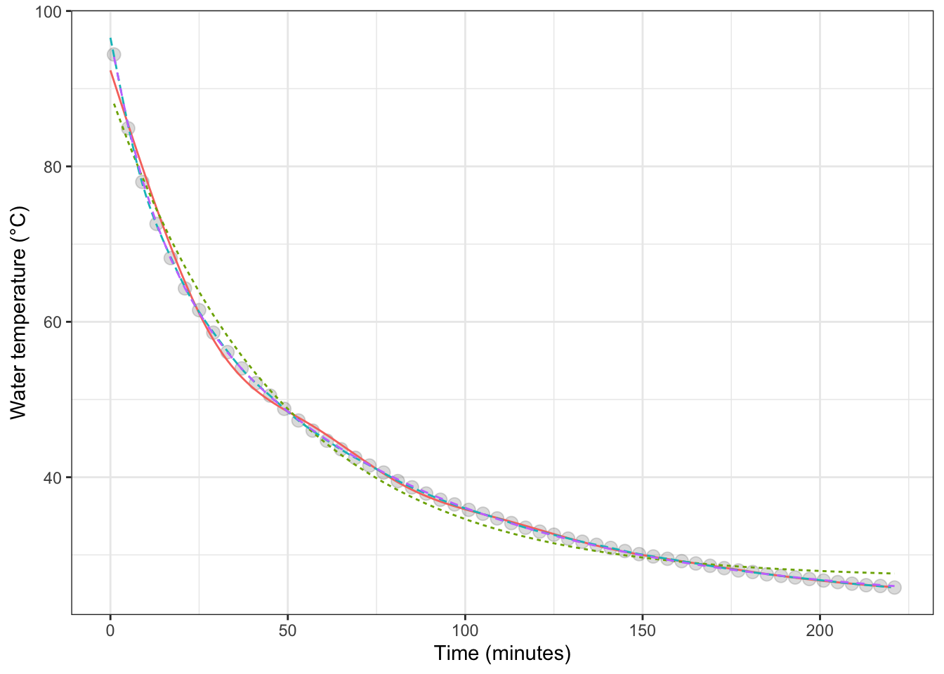
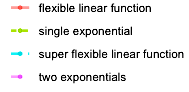
Figure 16.5: The model error – that is, the difference between the measured data and the model values – for each of the cooling water models shown in Figure 16.4.
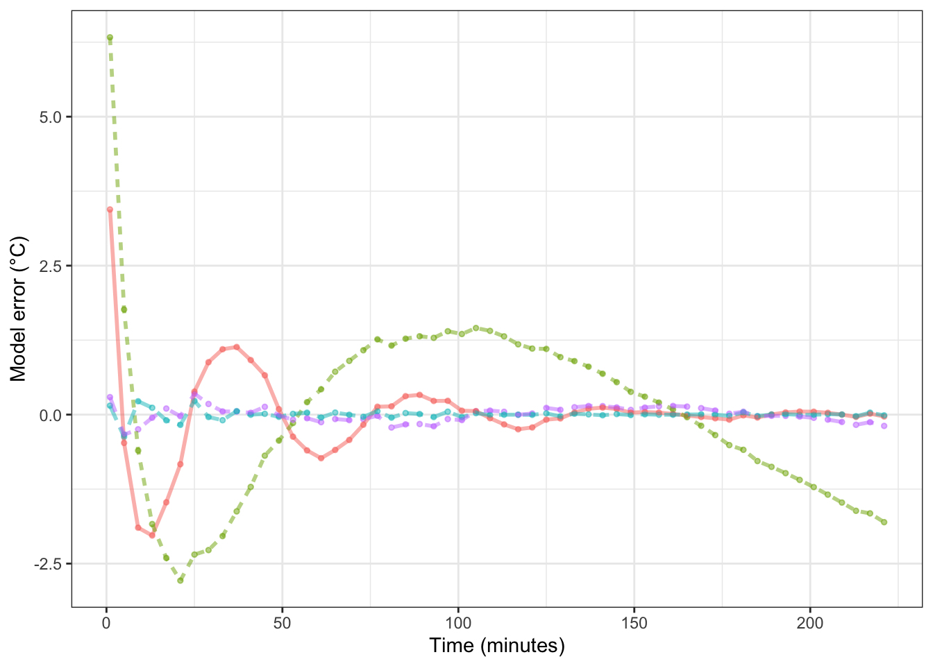
Table 16.4: The root mean square error (RMSE) for four different models of the temperature of water as it cools. The training data, not independent testing data, was used for the RMSE calculation
| model | RMSE |
|---|---|
| super flexible linear function | 0.0800 |
| two exponentials | 0.1309 |
| flexible linear function | 0.7259 |
| single exponential | 1.5003 |
To judge from solely from the RMSE, the super flexible linear function model is the best. In Chapter 18 we’ll examine the extent to which that result is due to using the training data for calculating the RMSE.
Keep in mind, though, that whether a model is good depends on the purpose for which it is being made. For a physicist, the purpose of building such a model would be to examine the physical mechanisms through which water cools. A one-exponential model corresponds to the water cooling because it is in contact with one other medium, such as the cup holding the water. A two-exponential model allows for the water to be in contact with two, different media: a fast process involving the cup and a slow process involving the room air, for instance. The RMSE for the two-exponential model is much smaller than for the one-exponential model, providing evidence that there are at least two, separate cooling mechanisms at work.
Среднеквадратичная ошибка (Mean Squared Error) – Среднее арифметическое (Mean) квадратов разностей между предсказанными и реальными значениями Модели (Model) Машинного обучения (ML):

Рассчитывается с помощью формулы, которая будет пояснена в примере ниже:
$$MSE = frac{1}{n} × sum_{i=1}^n (y_i — widetilde{y}_i)^2$$
$$MSEspace{}{–}space{Среднеквадратическая}space{ошибка,}$$
$$nspace{}{–}space{количество}space{наблюдений,}$$
$$y_ispace{}{–}space{фактическая}space{координата}space{наблюдения,}$$
$$widetilde{y}_ispace{}{–}space{предсказанная}space{координата}space{наблюдения,}$$
MSE практически никогда не равен нулю, и происходит это из-за элемента случайности в данных или неучитывания Оценочной функцией (Estimator) всех факторов, которые могли бы улучшить предсказательную способность.
Пример. Исследуем линейную регрессию, изображенную на графике выше, и установим величину среднеквадратической Ошибки (Error). Фактические координаты точек-Наблюдений (Observation) выглядят следующим образом:

Мы имеем дело с Линейной регрессией (Linear Regression), потому уравнение, предсказывающее положение записей, можно представить с помощью формулы:
$$y = M * x + b$$
$$yspace{–}space{значение}space{координаты}space{оси}space{y,}$$
$$Mspace{–}space{уклон}space{прямой}$$
$$xspace{–}space{значение}space{координаты}space{оси}space{x,}$$
$$bspace{–}space{смещение}space{прямой}space{относительно}space{начала}space{координат}$$
Параметры M и b уравнения нам, к счастью, известны в данном обучающем примере, и потому уравнение выглядит следующим образом:
$$y = 0,5252 * x + 17,306$$
Зная координаты реальных записей и уравнение линейной регрессии, мы можем восстановить полные координаты предсказанных наблюдений, обозначенных серыми точками на графике выше. Простой подстановкой значения координаты x в уравнение мы рассчитаем значение координаты ỹ:

Рассчитаем квадрат разницы между Y и Ỹ:

Сумма таких квадратов равна 4 445. Осталось только разделить это число на количество наблюдений (9):
$$MSE = frac{1}{9} × 4445 = 493$$
Само по себе число в такой ситуации становится показательным, когда Дата-сайентист (Data Scientist) предпринимает попытки улучшить предсказательную способность модели и сравнивает MSE каждой итерации, выбирая такое уравнение, что сгенерирует наименьшую погрешность в предсказаниях.
MSE и Scikit-learn
Среднеквадратическую ошибку можно вычислить с помощью SkLearn. Для начала импортируем функцию:
import sklearn
from sklearn.metrics import mean_squared_error
Инициализируем крошечные списки, содержащие реальные и предсказанные координаты y:
y_true = [5, 41, 70, 77, 134, 68, 138, 101, 131]
y_pred = [23, 35, 55, 90, 93, 103, 118, 121, 129]
Инициируем функцию mean_squared_error(), которая рассчитает MSE тем же способом, что и формула выше:
mean_squared_error(y_true, y_pred)
Интересно, что конечный результат на 3 отличается от расчетов с помощью Apple Numbers:
496.0Ноутбук, не требующий дополнительной настройки на момент написания статьи, можно скачать здесь.
Автор оригинальной статьи: @mmoshikoo
Фото: @tobyelliott
Среднеквадратичная ошибка прогноза
Из Википедии, бесплатной энциклопедии
Перейти к навигации
Перейти к поиску
В статистике средний квадрат ошибки предсказания или средний квадрат ошибки предсказания одного сглаживания или аппроксимации кривой процедуры является ожидаемое значение квадрата разности между подобранными значениями подразумевается прогнозирующей функциии значения (ненаблюдаемой) функции g . Это обратная мера объяснительной силыи может использоваться в процессе перекрестной проверки оценочной модели.
Если процедура сглаживания или аппроксимации имеет матрицу проекции (т.е. матрицу шляпы) L , которая отображает вектор наблюдаемых значений к вектору прогнозируемых значений с помощью тогда
MSPE можно разложить на два члена: среднее квадратов систематических ошибок подобранных значений и среднее значение дисперсии подобранных значений:
Знание g требуется для точного расчета MSPE; в противном случае его можно оценить.
Вычисление MSPE по данным вне выборки
Среднеквадратичная ошибка прогноза может быть вычислена точно в двух контекстах. Во- первых, с выборки данных длины п , то аналитик данных может запустить регрессии по сравнению только д точек данных (с д < п ), сдерживая другие п — д точек данных с конкретной целью их использования для вычисления оценка MSPE модели вне выборки (т. е. без использования данных, которые использовались в процессе оценки модели). Поскольку процесс регрессии адаптирован к q точкам в выборке, обычно MSPE в выборке будет меньше, чем MSPE вне выборки, вычисленной по n — qсдерживаемые точки. Если увеличение MSPE вне выборки по сравнению с в выборке относительно невелико, это приводит к положительному обзору модели. А если нужно сравнить две модели, то модель с более низким значением MSPE по сравнению с n — q точками данных вне выборки будет рассматриваться более благоприятно, независимо от относительных характеристик моделей в выборке. MSPE вне выборки в этом контексте является точным для точек данных вне выборки, по которым он был вычислен, но является просто оценкой MSPE модели для в основном ненаблюдаемой популяции, из которой были взяты данные.
Во-вторых, со временем аналитику данных может стать доступно больше данных, и тогда MSPE может быть вычислен на основе этих новых данных.
Оценка MSPE по населению
Когда модель была оценена по всем доступным данным без каких-либо задержек, MSPE модели по всей совокупности в основном ненаблюдаемых данных можно оценить следующим образом.
Для модели куда , можно написать
При использовании значений данных в выборке первый член справа эквивалентен
Таким образом,
Если известен или хорошо оценен , становится возможным оценить MSPE как
Колин Мэллоуз поддержал этот метод при построении своей статистики выбора модели C p , которая является нормализованной версией оцененной MSPE:
где p количество оцениваемых параметров p ивычисляется из версии модели, включающей все возможные регрессоры. Это завершает это доказательство.
См. Также
- Среднеквадратичная ошибка
- Ошибки и неточности в статистике
- Закон полной дисперсии
Дальнейшее чтение
- Пиндик, Роберт С .; Рубинфельд, Даниэль Л. (1991). «Прогнозирование с использованием моделей временных рядов». Эконометрические модели и экономические прогнозы (3-е изд.). Нью-Йорк: Макгроу-Хилл. С. 516–535 . ISBN 0-07-050098-3.
Accurately Measuring Model Prediction Error
May 2012
When assessing the quality of a model, being able to accurately measure its prediction error is of key importance. Often, however, techniques of measuring error are used that give grossly misleading results. This can lead to the phenomenon of over-fitting where a model may fit the training data very well, but will do a poor job of predicting results for new data not used in model training. Here is an overview of methods to accurately measure model prediction error.
When building prediction models, the primary goal should be to make a model that most accurately predicts the desired target value for new data. The measure of model error that is used should be one that achieves this goal. In practice, however, many modelers instead report a measure of model error that is based not on the error for new data but instead on the error the very same data that was used to train the model. The use of this incorrect error measure can lead to the selection of an inferior and inaccurate model.
Naturally, any model is highly optimized for the data it was trained on. The expected error the model exhibits on new data will always be higher than that it exhibits on the training data. As example, we could go out and sample 100 people and create a regression model to predict an individual’s happiness based on their wealth. We can record the squared error for how well our model does on this training set of a hundred people. If we then sampled a different 100 people from the population and applied our model to this new group of people, the squared error will almost always be higher in this second case.
It is helpful to illustrate this fact with an equation. We can develop a relationship between how well a model predicts on new data (its true prediction error and the thing we really care about) and how well it predicts on the training data (which is what many modelers in fact measure).
$$ True Prediction Error = Training Error + Training Optimism $$
Here, Training Optimism is basically a measure of how much worse our model does on new data compared to the training data. The more optimistic we are, the better our training error will be compared to what the true error is and the worse our training error will be as an approximation of the true error.
The Danger of Overfitting
In general, we would like to be able to make the claim that the optimism is constant for a given training set. If this were true, we could make the argument that the model that minimizes training error, will also be the model that will minimize the true prediction error for new data. As a consequence, even though our reported training error might be a bit optimistic, using it to compare models will cause us to still select the best model amongst those we have available. So we could in effect ignore the distinction between the true error and training errors for model selection purposes.
Unfortunately, this does not work. It turns out that the optimism is a function of model complexity: as complexity increases so does optimism. Thus we have a our relationship above for true prediction error becomes something like this:
$$ True Prediction Error = Training Error + f(Model Complexity) $$
How is the optimism related to model complexity? As model complexity increases (for instance by adding parameters terms in a linear regression) the model will always do a better job fitting the training data. This is a fundamental property of statistical models 1. In our happiness prediction model, we could use people’s middle initials as predictor variables and the training error would go down. We could use stock prices on January 1st, 1990 for a now bankrupt company, and the error would go down. We could even just roll dice to get a data series and the error would still go down. No matter how unrelated the additional factors are to a model, adding them will cause training error to decrease.
But at the same time, as we increase model complexity we can see a change in the true prediction accuracy (what we really care about). If we build a model for happiness that incorporates clearly unrelated factors such as stock ticker prices a century ago, we can say with certainty that such a model must necessarily be worse than the model without the stock ticker prices. Although the stock prices will decrease our training error (if very slightly), they conversely must also increase our prediction error on new data as they increase the variability of the model’s predictions making new predictions worse. Furthermore, even adding clearly relevant variables to a model can in fact increase the true prediction error if the signal to noise ratio of those variables is weak.
Let’s see what this looks like in practice. We can implement our wealth and happiness model as a linear regression. We can start with the simplest regression possible where $ Happiness=a+b Wealth+epsilon $ and then we can add polynomial terms to model nonlinear effects. Each polynomial term we add increases model complexity. So we could get an intermediate level of complexity with a quadratic model like $Happiness=a+b Wealth+c Wealth^2+epsilon$ or a high-level of complexity with a higher-order polynomial like $Happiness=a+b Wealth+c Wealth^2+d Wealth^3+e Wealth^4+f Wealth^5+g Wealth^6+epsilon$.
The figure below illustrates the relationship between the training error, the true prediction error, and optimism for a model like this. The scatter plots on top illustrate sample data with regressions lines corresponding to different levels of model complexity.
Training, optimism and true prediction error.
Increasing the model complexity will always decrease the model training error. At very high levels of complexity, we should be able to in effect perfectly predict every single point in the training data set and the training error should be near 0. Similarly, the true prediction error initially falls. The linear model without polynomial terms seems a little too simple for this data set. However, once we pass a certain point, the true prediction error starts to rise. At these high levels of complexity, the additional complexity we are adding helps us fit our training data, but it causes the model to do a worse job of predicting new data.
This is a case of overfitting the training data. In this region the model training algorithm is focusing on precisely matching random chance variability in the training set that is not present in the actual population. We can see this most markedly in the model that fits every point of the training data; clearly this is too tight a fit to the training data.
Preventing overfitting is a key to building robust and accurate prediction models. Overfitting is very easy to miss when only looking at the training error curve. To detect overfitting you need to look at the true prediction error curve. Of course, it is impossible to measure the exact true prediction curve (unless you have the complete data set for your entire population), but there are many different ways that have been developed to attempt to estimate it with great accuracy. The second section of this work will look at a variety of techniques to accurately estimate the model’s true prediction error.
An Example of the Cost of Poorly Measuring Error
Let’s look at a fairly common modeling workflow and use it to illustrate the pitfalls of using training error in place of the true prediction error 2. We’ll start by generating 100 simulated data points. Each data point has a target value we are trying to predict along with 50 different parameters. For instance, this target value could be the growth rate of a species of tree and the parameters are precipitation, moisture levels, pressure levels, latitude, longitude, etc. In this case however, we are going to generate every single data point completely randomly. Each number in the data set is completely independent of all the others, and there is no relationship between any of them.
For this data set, we create a linear regression model where we predict the target value using the fifty regression variables. Since we know everything is unrelated we would hope to find an R2 of 0. Unfortunately, that is not the case and instead we find an R2 of 0.5. That’s quite impressive given that our data is pure noise! However, we want to confirm this result so we do an F-test. This test measures the statistical significance of the overall regression to determine if it is better than what would be expected by chance. Using the F-test we find a p-value of 0.53. This indicates our regression is not significant.
If we stopped there, everything would be fine; we would throw out our model which would be the right choice (it is pure noise after all!). However, a common next step would be to throw out only the parameters that were poor predictors, keep the ones that are relatively good predictors and run the regression again. Let’s say we kept the parameters that were significant at the 25% level of which there are 21 in this example case. Then we rerun our regression.
In this second regression we would find:
- An R2 of 0.36
- A p-value of 5*10-4
- 6 parameters significant at the 5% level
Again, this data was pure noise; there was absolutely no relationship in it. But from our data we find a highly significant regression, a respectable R2 (which can be very high compared to those found in some fields like the social sciences) and 6 significant parameters!
This is quite a troubling result, and this procedure is not an uncommon one but clearly leads to incredibly misleading results. It shows how easily statistical processes can be heavily biased if care to accurately measure error is not taken.
Methods of Measuring Error
Adjusted R2
The R2 measure is by far the most widely used and reported measure of error and goodness of fit. R2 is calculated quite simply. First the proposed regression model is trained and the differences between the predicted and observed values are calculated and squared. These squared errors are summed and the result is compared to the sum of the squared errors generated using the null model. The null model is a model that simply predicts the average target value regardless of what the input values for that point are. The null model can be thought of as the simplest model possible and serves as a benchmark against which to test other models. Mathematically:
$$ R^2 = 1 — frac{Sum of Squared Errors Model}{Sum of Squared Errors Null Model} $$
R2 has very intuitive properties. When our model does no better than the null model then R2 will be 0. When our model makes perfect predictions, R2 will be 1. R2 is an easy to understand error measure that is in principle generalizable across all regression models.
Commonly, R2 is only applied as a measure of training error. This is unfortunate as we saw in the above example how you can get high R2 even with data that is pure noise. In fact there is an analytical relationship to determine the expected R2 value given a set of n observations and p parameters each of which is pure noise:
$$Eleft[R^2right]=frac{p}{n}$$
So if you incorporate enough data in your model you can effectively force whatever level of R2 you want regardless of what the true relationship is. In our illustrative example above with 50 parameters and 100 observations, we would expect an R2 of 50/100 or 0.5.
One attempt to adjust for this phenomenon and penalize additional complexity is Adjusted R2. Adjusted R2 reduces R2 as more parameters are added to the model. There is a simple relationship between adjusted and regular R2:
$$Adjusted R^2=1-(1-R^2)frac{n-1}{n-p-1}$$
Unlike regular R2, the error predicted by adjusted R2 will start to increase as model complexity becomes very high. Adjusted R2 is much better than regular R2 and due to this fact, it should always be used in place of regular R2. However, adjusted R2 does not perfectly match up with the true prediction error. In fact, adjusted R2 generally under-penalizes complexity. That is, it fails to decrease the prediction accuracy as much as is required with the addition of added complexity.
Given this, the usage of adjusted R2 can still lead to overfitting. Furthermore, adjusted R2 is based on certain parametric assumptions that may or may not be true in a specific application. This can further lead to incorrect conclusions based on the usage of adjusted R2.
Pros
- Easy to apply
- Built into most existing analysis programs
- Fast to compute
- Easy to interpret 3
Cons
- Less generalizable
- May still overfit the data
Information Theoretic Approaches
There are a variety of approaches which attempt to measure model error as how much information is lost between a candidate model and the true model. Of course the true model (what was actually used to generate the data) is unknown, but given certain assumptions we can still obtain an estimate of the difference between it and and our proposed models. For a given problem the more this difference is, the higher the error and the worse the tested model is.
Information theoretic approaches assume a parametric model. Given a parametric model, we can define the likelihood of a set of data and parameters as the, colloquially, the probability of observing the data given the parameters 4. If we adjust the parameters in order to maximize this likelihood we obtain the maximum likelihood estimate of the parameters for a given model and data set. We can then compare different models and differing model complexities using information theoretic approaches to attempt to determine the model that is closest to the true model accounting for the optimism.
The most popular of these the information theoretic techniques is Akaike’s Information Criteria (AIC). It can be defined as a function of the likelihood of a specific model and the number of parameters in that model:
$$ AIC = -2 ln(Likelihood) + 2p $$
Like other error criteria, the goal is to minimize the AIC value. The AIC formulation is very elegant. The first part ($-2 ln(Likelihood)$) can be thought of as the training set error rate and the second part ($2p$) can be though of as the penalty to adjust for the optimism.
However, in addition to AIC there are a number of other information theoretic equations that can be used. The two following examples are different information theoretic criteria with alternative derivations. In these cases, the optimism adjustment has different forms and depends on the number of sample size (n).
$$ AICc = -2 ln(Likelihood) + 2p + frac{2p(p+1)}{n-p-1} $$
$$ BIC = -2 ln(Likelihood) + p ln(n) $$
The choice of which information theoretic approach to use is a very complex one and depends on a lot of specific theory, practical considerations and sometimes even philosophical ones. This can make the application of these approaches often a leap of faith that the specific equation used is theoretically suitable to a specific data and modeling problem.
Pros
- Easy to apply
- Built into most advanced analysis programs
Cons
- Metric not comparable between different applications
- Requires a model that can generate likelihoods 5
- Various forms a topic of theoretical debate within the academic field
Holdout Set
Both the preceding techniques are based on parametric and theoretical assumptions. If these assumptions are incorrect for a given data set then the methods will likely give erroneous results. Fortunately, there exists a whole separate set of methods to measure error that do not make these assumptions and instead use the data itself to estimate the true prediction error.
The simplest of these techniques is the holdout set method. Here we initially split our data into two groups. One group will be used to train the model; the second group will be used to measure the resulting model’s error. For instance, if we had 1000 observations, we might use 700 to build the model and the remaining 300 samples to measure that model’s error.
Holdout data split.
This technique is really a gold standard for measuring the model’s true prediction error. As defined, the model’s true prediction error is how well the model will predict for new data. By holding out a test data set from the beginning we can directly measure this.
The cost of the holdout method comes in the amount of data that is removed from the model training process. For instance, in the illustrative example here, we removed 30% of our data. This means that our model is trained on a smaller data set and its error is likely to be higher than if we trained it on the full data set. The standard procedure in this case is to report your error using the holdout set, and then train a final model using all your data. The reported error is likely to be conservative in this case, with the true error of the full model actually being lower. Such conservative predictions are almost always more useful in practice than overly optimistic predictions.
One key aspect of this technique is that the holdout data must truly not be analyzed until you have a final model. A common mistake is to create a holdout set, train a model, test it on the holdout set, and then adjust the model in an iterative process. If you repeatedly use a holdout set to test a model during development, the holdout set becomes contaminated. Its data has been used as part of the model selection process and it no longer gives unbiased estimates of the true model prediction error.
Pros
- No parametric or theoretic assumptions
- Given enough data, highly accurate
- Very simple to implement
- Conceptually simple
Cons
- Potential conservative bias
- Tempting to use the holdout set prior to model completion resulting in contamination
- Must choose the size of the holdout set (70%-30% is a common split)
Cross-Validation and Resampling
In some cases the cost of setting aside a significant portion of the data set like the holdout method requires is too high. As a solution, in these cases a resampling based technique such as cross-validation may be used instead.
Cross-validation works by splitting the data up into a set of n folds. So, for example, in the case of 5-fold cross-validation with 100 data points, you would create 5 folds each containing 20 data points. Then the model building and error estimation process is repeated 5 times. Each time four of the groups are combined (resulting in 80 data points) and used to train your model. Then the 5th group of 20 points that was not used to construct the model is used to estimate the true prediction error. In the case of 5-fold cross-validation you would end up with 5 error estimates that could then be averaged to obtain a more robust estimate of the true prediction error.
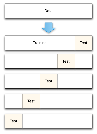
5-Fold cross-validation data split.
As can be seen, cross-validation is very similar to the holdout method. Where it differs, is that each data point is used both to train models and to test a model, but never at the same time. Where data is limited, cross-validation is preferred to the holdout set as less data must be set aside in each fold than is needed in the pure holdout method. Cross-validation can also give estimates of the variability of the true error estimation which is a useful feature. However, if understanding this variability is a primary goal, other resampling methods such as Bootstrapping are generally superior.
On important question of cross-validation is what number of folds to use. Basically, the smaller the number of folds, the more biased the error estimates (they will be biased to be conservative indicating higher error than there is in reality) but the less variable they will be. On the extreme end you can have one fold for each data point which is known as Leave-One-Out-Cross-Validation. In this case, your error estimate is essentially unbiased but it could potentially have high variance. Understanding the Bias-Variance Tradeoff is important when making these decisions. Another factor to consider is computational time which increases with the number of folds. For each fold you will have to train a new model, so if this process is slow, it might be prudent to use a small number of folds. Ultimately, it appears that, in practice, 5-fold or 10-fold cross-validation are generally effective fold sizes.
Pros
- No parametric or theoretic assumptions
- Given enough data, highly accurate
- Conceptually simple
Cons
- Computationally intensive
- Must choose the fold size
- Potential conservative bias
Making a Choice
In summary, here are some techniques you can use to more accurately measure model prediction error:
- Adjusted R2
- Information Theoretic Techniques
- Holdout Sample
- Cross-Validation and Resampling Methods
A fundamental choice a modeler must make is whether they want to rely on theoretic and parametric assumptions to adjust for the optimism like the first two methods require. Alternatively, does the modeler instead want to use the data itself in order to estimate the optimism.
Generally, the assumption based methods are much faster to apply, but this convenience comes at a high cost. First, the assumptions that underly these methods are generally wrong. How wrong they are and how much this skews results varies on a case by case basis. The error might be negligible in many cases, but fundamentally results derived from these techniques require a great deal of trust on the part of evaluators that this error is small.
Ultimately, in my own work I prefer cross-validation based approaches. Cross-validation provides good error estimates with minimal assumptions. The primary cost of cross-validation is computational intensity but with the rapid increase in computing power, this issue is becoming increasingly marginal. At its root, the cost with parametric assumptions is that even though they are acceptable in most cases, there is no clear way to show their suitability for a specific case. Thus their use provides lines of attack to critique a model and throw doubt on its results. Although cross-validation might take a little longer to apply initially, it provides more confidence and security in the resulting conclusions.
❧