Среднее арифметическое значение, средняя квадратичная и средняя арифметическая погрешности измеряемой величины
Первой величиной,
которую приходится вычислять при
обработке результатов опытов, является
среднее арифметическое из результатов
ряда измерений, которое определяется
по формуле (6).
Практически число
измерений всегда ограничено, поэтому
среднее арифметическое ![]()
не равно
истинному значению измеряемой величины
![]() ,
,
но будет
тем ближе к нему, чем больше число
выполненных измерений ![]() .
.
В теории
вероятностей доказывается, что среднее
арифметическое из результатов отдельных
измерений является наиболее вероятным
значением измеряемой величины. Это
утверждение справедливо при условии,
когда все
измерения равноточные, а распределение
погрешности измерений подчиняется
вышеупомянутому закону распределения—
закону Гаусса.
Если вместо
истинного значения неизвестной величины
использовать среднее арифметическое
![]() ,
,
тогда на
основании равенства (1) имеем:
 (11)
(11)
В (11) погрешность
![]() несколько
несколько
отличается от истинной и называется
абсолютной погрешностью единичного
измерения
![]() (12)
(12)
Лучшим из критериев
для оценки погрешностей результатов
измерений является средняя квадратичная
погрешность, которая характеризует
степень (меру) рассеяния результатов
отдельных измерений
около среднего
их значения. Для определения
среднеквадратической погрешности
единичных измерений при ограниченном
числе опытов используется формула (7),
которая с учетом (12) записывается в виде:
 . (13)
Средняя квадратическая
погрешность, вычисляемая по формуле
(13), характеризует погрешность единичного
результата из всего ряда n
измерений.
Как уже отмечалось,
при увеличении числа n
измерений наблюдается взаимная
компенсация случайных ошибок. Поэтому
усредненная средняя квадратичная
погрешность![]() ,
,
определяемая по формуле (9) и характеризующая
окончательный результат измерений,
уменьшается при увеличении числаn
повторных
измерений искомой величины. Поскольку
вычисления величины
![]() достаточно громоздки, то в ряде случаев
достаточно громоздки, то в ряде случаев
(если не оговорено в условиях решаемой
задачи) для оценки ошибки, допущенной
при определении средней величины,
пользуются средней арифметической
погрешностью, которая вычисляется как
средняя величина всех величин абсолютных
погрешностей единичных измерений (12),
взятых по модулю:
![]() .
.
(14)
Так как суммирование
в (14) выполняется без учета знака ![]() ,
,
то формула (14) даёт среднее значение
максимальной возможной погрешности.
Вопрос о том, какой
формулой пользоваться при оценке
измерений, решается при планировании
эксперимента. Считается, что при числе
измерений меньше пяти можно ограничиться
вычислением средней абсолютной
погрешности по формуле (14).
Средняя абсолютная
погрешность даёт возможность указать
пределы (интервал), внутри которых
заключено истинное значение измеряемой
величины.
Сама по себе
абсолютная погрешность не даёт достаточно
наглядного представления о степени
точности измерения, поэтому для оценки
точности результата применяется
относительная погрешность. Относительная
погрешность величины x
при ограниченном числе опытов вычисляется
по формуле:
![]() .
.
(15)
From Wikipedia, the free encyclopedia
In statistics, mean absolute error (MAE) is a measure of errors between paired observations expressing the same phenomenon. Examples of Y versus X include comparisons of predicted versus observed, subsequent time versus initial time, and one technique of measurement versus an alternative technique of measurement. MAE is calculated as the sum of absolute errors divided by the sample size:[1]

It is thus an arithmetic average of the absolute errors  , where
  is the prediction and
  the true value. Note that alternative formulations may include relative frequencies as weight factors. The mean absolute error uses the same scale as the data being measured. This is known as a scale-dependent accuracy measure and therefore cannot be used to make comparisons between series using different scales.[2] The mean absolute error is a common measure of forecast error in time series analysis,[3] sometimes used in confusion with the more standard definition of mean absolute deviation. The same confusion exists more generally.
Quantity disagreement and allocation disagreement[edit]
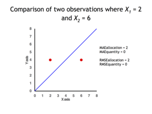
2 data points for which Quantity Disagreement is 0 and Allocation Disagreement is 2 for both MAE and RMSE
It is possible to express MAE as the sum of two components: Quantity Disagreement and Allocation Disagreement. Quantity Disagreement is the absolute value of the Mean Error given by:[4]

Allocation Disagreement is MAE minus Quantity Disagreement.
It is also possible to identify the types of difference by looking at an  plot. Quantity difference exists when the average of the X values does not equal the average of the Y values. Allocation difference exists if and only if points reside on both sides of the identity line.[4][5]
[edit]
The mean absolute error is one of a number of ways of comparing forecasts with their eventual outcomes. Well-established alternatives are the mean absolute scaled error (MASE) and the mean squared error. These all summarize performance in ways that disregard the direction of over- or under- prediction; a measure that does place emphasis on this is the mean signed difference.
Where a prediction model is to be fitted using a selected performance measure, in the sense that the least squares approach is related to the mean squared error, the equivalent for mean absolute error is least absolute deviations.
MAE is not identical to root-mean square error (RMSE), although some researchers report and interpret it that way. MAE is conceptually simpler and also easier to interpret than RMSE: it is simply the average absolute vertical or horizontal distance between each point in a scatter plot and the Y=X line. In other words, MAE is the average absolute difference between X and Y. Furthermore, each error contributes to MAE in proportion to the absolute value of the error. This is in contrast to RMSE which involves squaring the differences, so that a few large differences will increase the RMSE to a greater degree than the MAE.[4] See the example above for an illustration of these differences.
Optimality property[edit]
The mean absolute error of a real variable c with respect to the random variable X is

Provided that the probability distribution of X is such that the above expectation exists, then m is a median of X if and only if m is a minimizer of the mean absolute error with respect to X.[6] In particular, m is a sample median if and only if m minimizes the arithmetic mean of the absolute deviations.[7]
More generally, a median is defined as a minimum of

as discussed at Multivariate median (and specifically at Spatial median).
This optimization-based definition of the median is useful in statistical data-analysis, for example, in k-medians clustering.
Proof of optimality[edit]
Statement: The classifier minimising  is
is  .
.
Proof:
The Loss functions for classification is
![{displaystyle {begin{aligned}L&=mathbb {E} [|y-a||X=x]\&=int _{-infty }^{infty }|y-a|f_{Y|X}(y),dy\&=int _{-infty }^{a}(a-y)f_{Y|X}(y),dy+int _{a}^{infty }(y-a)f_{Y|X}(y),dy\end{aligned}}}](https://wikimedia.org/api/rest_v1/media/math/render/svg/7e953e54457072620a7c2764db0801f69c4e883d)
Differentiating with respect to a gives

This means

Hence

See also[edit]
- Least absolute deviations
- Mean absolute percentage error
- Mean percentage error
- Symmetric mean absolute percentage error
References[edit]
- ^ Willmott, Cort J.; Matsuura, Kenji (December 19, 2005). «Advantages of the mean absolute error (MAE) over the root mean square error (RMSE) in assessing average model performance». Climate Research. 30: 79–82. doi:10.3354/cr030079.
- ^ «2.5 Evaluating forecast accuracy | OTexts». www.otexts.org. Retrieved 2016-05-18.
- ^ Hyndman, R. and Koehler A. (2005). «Another look at measures of forecast accuracy» [1]
- ^ a b c Pontius Jr., Robert Gilmore; Thontteh, Olufunmilayo; Chen, Hao (2008). «Components of information for multiple resolution comparison between maps that share a real variable». Environmental and Ecological Statistics. 15 (2): 111–142. doi:10.1007/s10651-007-0043-y. S2CID 21427573.
- ^ Willmott, C. J.; Matsuura, K. (January 2006). «On the use of dimensioned measures of error to evaluate the performance of spatial interpolators». International Journal of Geographical Information Science. 20: 89–102. doi:10.1080/13658810500286976. S2CID 15407960.
- ^ Stroock, Daniel (2011). Probability Theory. Cambridge University Press. pp. 43. ISBN 978-0-521-13250-3.
- ^ Nicolas, André (2012-02-25). «The Median Minimizes the Sum of Absolute Deviations (The $ {L}_{1} $ Norm)». StackExchange.
From Wikipedia, the free encyclopedia
In statistics, mean absolute error (MAE) is a measure of errors between paired observations expressing the same phenomenon. Examples of Y versus X include comparisons of predicted versus observed, subsequent time versus initial time, and one technique of measurement versus an alternative technique of measurement. MAE is calculated as the sum of absolute errors divided by the sample size:[1]
It is thus an arithmetic average of the absolute errors , where is the prediction and the true value. Note that alternative formulations may include relative frequencies as weight factors. The mean absolute error uses the same scale as the data being measured. This is known as a scale-dependent accuracy measure and therefore cannot be used to make comparisons between series using different scales.[2] The mean absolute error is a common measure of forecast error in time series analysis,[3] sometimes used in confusion with the more standard definition of mean absolute deviation. The same confusion exists more generally.
Quantity disagreement and allocation disagreement[edit]
2 data points for which Quantity Disagreement is 0 and Allocation Disagreement is 2 for both MAE and RMSE
It is possible to express MAE as the sum of two components: Quantity Disagreement and Allocation Disagreement. Quantity Disagreement is the absolute value of the Mean Error given by:[4]
Allocation Disagreement is MAE minus Quantity Disagreement.
It is also possible to identify the types of difference by looking at an plot. Quantity difference exists when the average of the X values does not equal the average of the Y values. Allocation difference exists if and only if points reside on both sides of the identity line.[4][5]
[edit]
The mean absolute error is one of a number of ways of comparing forecasts with their eventual outcomes. Well-established alternatives are the mean absolute scaled error (MASE) and the mean squared error. These all summarize performance in ways that disregard the direction of over- or under- prediction; a measure that does place emphasis on this is the mean signed difference.
Where a prediction model is to be fitted using a selected performance measure, in the sense that the least squares approach is related to the mean squared error, the equivalent for mean absolute error is least absolute deviations.
MAE is not identical to root-mean square error (RMSE), although some researchers report and interpret it that way. MAE is conceptually simpler and also easier to interpret than RMSE: it is simply the average absolute vertical or horizontal distance between each point in a scatter plot and the Y=X line. In other words, MAE is the average absolute difference between X and Y. Furthermore, each error contributes to MAE in proportion to the absolute value of the error. This is in contrast to RMSE which involves squaring the differences, so that a few large differences will increase the RMSE to a greater degree than the MAE.[4] See the example above for an illustration of these differences.
Optimality property[edit]
The mean absolute error of a real variable c with respect to the random variable X is
Provided that the probability distribution of X is such that the above expectation exists, then m is a median of X if and only if m is a minimizer of the mean absolute error with respect to X.[6] In particular, m is a sample median if and only if m minimizes the arithmetic mean of the absolute deviations.[7]
More generally, a median is defined as a minimum of
as discussed at Multivariate median (and specifically at Spatial median).
This optimization-based definition of the median is useful in statistical data-analysis, for example, in k-medians clustering.
Proof of optimality[edit]
Statement: The classifier minimising is .
Proof:
The Loss functions for classification is
Differentiating with respect to a gives
This means
Hence
See also[edit]
- Least absolute deviations
- Mean absolute percentage error
- Mean percentage error
- Symmetric mean absolute percentage error
References[edit]
- ^ Willmott, Cort J.; Matsuura, Kenji (December 19, 2005). «Advantages of the mean absolute error (MAE) over the root mean square error (RMSE) in assessing average model performance». Climate Research. 30: 79–82. doi:10.3354/cr030079.
- ^ «2.5 Evaluating forecast accuracy | OTexts». www.otexts.org. Retrieved 2016-05-18.
- ^ Hyndman, R. and Koehler A. (2005). «Another look at measures of forecast accuracy» [1]
- ^ a b c Pontius Jr., Robert Gilmore; Thontteh, Olufunmilayo; Chen, Hao (2008). «Components of information for multiple resolution comparison between maps that share a real variable». Environmental and Ecological Statistics. 15 (2): 111–142. doi:10.1007/s10651-007-0043-y. S2CID 21427573.
- ^ Willmott, C. J.; Matsuura, K. (January 2006). «On the use of dimensioned measures of error to evaluate the performance of spatial interpolators». International Journal of Geographical Information Science. 20: 89–102. doi:10.1080/13658810500286976. S2CID 15407960.
- ^ Stroock, Daniel (2011). Probability Theory. Cambridge University Press. pp. 43. ISBN 978-0-521-13250-3.
- ^ Nicolas, André (2012-02-25). «The Median Minimizes the Sum of Absolute Deviations (The $ {L}_{1} $ Norm)». StackExchange.