The mean squared error is a common way to measure the prediction accuracy of a model. In this tutorial, you’ll learn how to calculate the mean squared error in Python. You’ll start off by learning what the mean squared error represents. Then you’ll learn how to do this using Scikit-Learn (sklean), Numpy, as well as from scratch.
What is the Mean Squared Error
The mean squared error measures the average of the squares of the errors. What this means, is that it returns the average of the sums of the square of each difference between the estimated value and the true value.
The MSE is always positive, though it can be 0 if the predictions are completely accurate. It incorporates the variance of the estimator (how widely spread the estimates are) and its bias (how different the estimated values are from their true values).
The formula looks like below:

Now that you have an understanding of how to calculate the MSE, let’s take a look at how it can be calculated using Python.
Interpreting the Mean Squared Error
The mean squared error is always 0 or positive. When a MSE is larger, this is an indication that the linear regression model doesn’t accurately predict the model.
An important piece to note is that the MSE is sensitive to outliers. This is because it calculates the average of every data point’s error. Because of this, a larger error on outliers will amplify the MSE.
There is no “target” value for the MSE. The MSE can, however, be a good indicator of how well a model fits your data. It can also give you an indicator of choosing one model over another.
Loading a Sample Pandas DataFrame
Let’s start off by loading a sample Pandas DataFrame. If you want to follow along with this tutorial line-by-line, simply copy the code below and paste it into your favorite code editor.
# Importing a sample Pandas DataFrame
import pandas as pd

df = pd.DataFrame.from_dict({
    'x': [1,2,3,4,5,6,7,8,9,10],
    'y': [1,2,2,4,4,5,6,7,9,10]})

print(df.head())
#    x  y
# 0  1  1
# 1  2  2
# 2  3  2
# 3  4  4
# 4  5  4
You can see that the editor has loaded a DataFrame containing values for variables x and y. We can plot this data out, including the line of best fit using Seaborn’s .regplot() function:
# Plotting a line of best fit
import seaborn as sns
import matplotlib.pyplot as plt
sns.regplot(data=df, x='x', y='y', ci=None)
plt.ylim(bottom=0)
plt.xlim(left=0)
plt.show()
This returns the following visualization:
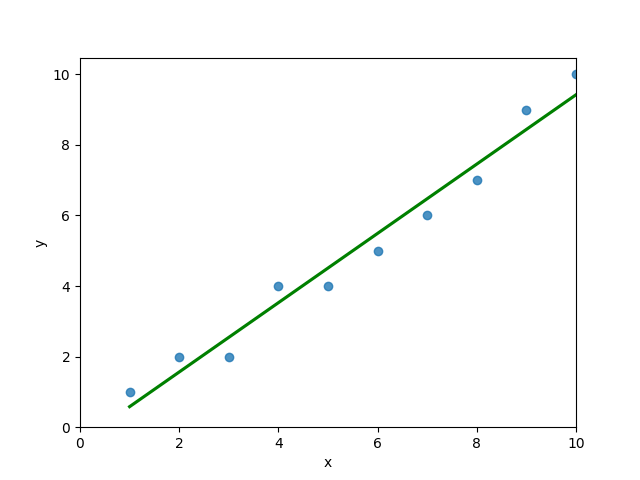
The mean squared error calculates the average of the sum of the squared differences between a data point and the line of best fit. By virtue of this, the lower a mean sqared error, the more better the line represents the relationship.
We can calculate this line of best using Scikit-Learn. You can learn about this in this in-depth tutorial on linear regression in sklearn. The code below predicts values for each x value using the linear model:
# Calculating prediction y values in sklearn
from sklearn.linear_model import LinearRegression

model = LinearRegression()
model.fit(df[['x']], df['y'])
y_2 = model.predict(df[['x']])
df['y_predicted'] = y_2
print(df.head())

# Returns:
#    x  y  y_predicted
# 0  1  1     0.581818
# 1  2  2     1.563636
# 2  3  2     2.545455
# 3  4  4     3.527273
# 4  5  4     4.509091
Calculating the Mean Squared Error with Scikit-Learn
The simplest way to calculate a mean squared error is to use Scikit-Learn (sklearn). The metrics module comes with a function, mean_squared_error() which allows you to pass in true and predicted values.
Let’s see how to calculate the MSE with sklearn:
# Calculating the MSE with sklearn
from sklearn.metrics import mean_squared_error
mse = mean_squared_error(df['y'], df['y_predicted'])
print(mse)

# Returns: 0.24727272727272714
This approach works very well when you’re already importing Scikit-Learn. That said, the function works easily on a Pandas DataFrame, as shown above.
In the next section, you’ll learn how to calculate the MSE with Numpy using a custom function.
Calculating the Mean Squared Error from Scratch using Numpy
Numpy itself doesn’t come with a function to calculate the mean squared error, but you can easily define a custom function to do this. We can make use of the subtract() function to subtract arrays element-wise.
# Definiting a custom function to calculate the MSE
import numpy as np

def mse(actual, predicted):
    actual = np.array(actual)
    predicted = np.array(predicted)
    differences = np.subtract(actual, predicted)
    squared_differences = np.square(differences)
    return squared_differences.mean()

print(mse(df['y'], df['y_predicted']))

# Returns: 0.24727272727272714
The code above is a bit verbose, but it shows how the function operates. We can cut down the code significantly, as shown below:
# A shorter version of the code above
import numpy as np

def mse(actual, predicted):
    return np.square(np.subtract(np.array(actual), np.array(predicted))).mean()

print(mse(df['y'], df['y_predicted']))

# Returns: 0.24727272727272714
Conclusion
In this tutorial, you learned what the mean squared error is and how it can be calculated using Python. First, you learned how to use Scikit-Learn’s mean_squared_error() function and then you built a custom function using Numpy.
The MSE is an important metric to use in evaluating the performance of your machine learning models. While Scikit-Learn abstracts the way in which the metric is calculated, understanding how it can be implemented from scratch can be a helpful tool.
Additional Resources
To learn more about related topics, check out the tutorials below:
- Pandas Variance: Calculating Variance of a Pandas Dataframe Column
- Calculate the Pearson Correlation Coefficient in Python
- How to Calculate a Z-Score in Python (4 Ways)
- Official Documentation from Scikit-Learn
Перевод
Ссылка на автора
Показатели эффективности прогнозирования по временным рядам дают сводку об умениях и возможностях модели прогноза, которая сделала прогнозы.
Есть много разных показателей производительности на выбор. Может быть непонятно, какую меру использовать и как интерпретировать результаты.
В этом руководстве вы узнаете показатели производительности для оценки прогнозов временных рядов с помощью Python.
Временные ряды, как правило, фокусируются на прогнозировании реальных значений, называемых проблемами регрессии. Поэтому показатели эффективности в этом руководстве будут сосредоточены на методах оценки реальных прогнозов.
После завершения этого урока вы узнаете:
- Основные показатели выполнения прогноза, включая остаточную ошибку прогноза и смещение прогноза.
- Вычисления ошибок прогноза временного ряда, которые имеют те же единицы, что и ожидаемые результаты, такие как средняя абсолютная ошибка.
- Широко используются вычисления ошибок, которые наказывают большие ошибки, такие как среднеквадратическая ошибка и среднеквадратичная ошибка.
Давайте начнем.

Ошибка прогноза (или остаточная ошибка прогноза)
ошибка прогноза рассчитывается как ожидаемое значение минус прогнозируемое значение.
Это называется остаточной ошибкой прогноза.
forecast_error = expected_value - predicted_valueОшибка прогноза может быть рассчитана для каждого прогноза, предоставляя временной ряд ошибок прогноза.
В приведенном ниже примере показано, как можно рассчитать ошибку прогноза для серии из 5 прогнозов по сравнению с 5 ожидаемыми значениями. Пример был придуман для демонстрационных целей.
expected = [0.0, 0.5, 0.0, 0.5, 0.0]
predictions = [0.2, 0.4, 0.1, 0.6, 0.2]
forecast_errors = [expected[i]-predictions[i] for i in range(len(expected))]
print('Forecast Errors: %s' % forecast_errors)
При выполнении примера вычисляется ошибка прогноза для каждого из 5 прогнозов. Список ошибок прогноза затем печатается.
Forecast Errors: [-0.2, 0.09999999999999998, -0.1, -0.09999999999999998, -0.2]Единицы ошибки прогноза совпадают с единицами прогноза. Ошибка прогноза, равная нулю, означает отсутствие ошибки или совершенный навык для этого прогноза.
Средняя ошибка прогноза (или ошибка прогноза)
Средняя ошибка прогноза рассчитывается как среднее значение ошибки прогноза.
mean_forecast_error = mean(forecast_error)Ошибки прогноза могут быть положительными и отрицательными. Это означает, что при вычислении среднего из этих значений идеальная средняя ошибка прогноза будет равна нулю.
Среднее значение ошибки прогноза, отличное от нуля, указывает на склонность модели к превышению прогноза (положительная ошибка) или занижению прогноза (отрицательная ошибка). Таким образом, средняя ошибка прогноза также называется прогноз смещения,
Ошибка прогноза может быть рассчитана непосредственно как среднее значение прогноза. В приведенном ниже примере показано, как среднее значение ошибок прогноза может быть рассчитано вручную.
expected = [0.0, 0.5, 0.0, 0.5, 0.0]
predictions = [0.2, 0.4, 0.1, 0.6, 0.2]
forecast_errors = [expected[i]-predictions[i] for i in range(len(expected))]
bias = sum(forecast_errors) * 1.0/len(expected)
print('Bias: %f' % bias)
При выполнении примера выводится средняя ошибка прогноза, также известная как смещение прогноза.
Bias: -0.100000Единицы смещения прогноза совпадают с единицами прогнозов. Прогнозируемое смещение нуля или очень маленькое число около нуля показывает несмещенную модель.
Средняя абсолютная ошибка
средняя абсолютная ошибка или MAE, рассчитывается как среднее значение ошибок прогноза, где все значения прогноза вынуждены быть положительными.
Заставить ценности быть положительными называется сделать их абсолютными. Это обозначено абсолютной функциейабс ()или математически показано как два символа канала вокруг значения:| Значение |,
mean_absolute_error = mean( abs(forecast_error) )кудаабс ()делает ценности позитивными,forecast_errorодна или последовательность ошибок прогноза, иимею в виду()рассчитывает среднее значение.
Мы можем использовать mean_absolute_error () функция из библиотеки scikit-learn для вычисления средней абсолютной ошибки для списка прогнозов. Пример ниже демонстрирует эту функцию.
from sklearn.metrics import mean_absolute_error
expected = [0.0, 0.5, 0.0, 0.5, 0.0]
predictions = [0.2, 0.4, 0.1, 0.6, 0.2]
mae = mean_absolute_error(expected, predictions)
print('MAE: %f' % mae)
При выполнении примера вычисляется и выводится средняя абсолютная ошибка для списка из 5 ожидаемых и прогнозируемых значений.
MAE: 0.140000Эти значения ошибок приведены в исходных единицах прогнозируемых значений. Средняя абсолютная ошибка, равная нулю, означает отсутствие ошибки.
Средняя квадратическая ошибка
средняя квадратическая ошибка или MSE, рассчитывается как среднее значение квадратов ошибок прогноза. Возведение в квадрат значений ошибки прогноза заставляет их быть положительными; это также приводит к большему количеству ошибок.
Квадратные ошибки прогноза с очень большими или выбросами возводятся в квадрат, что, в свою очередь, приводит к вытягиванию среднего значения квадратов ошибок прогноза, что приводит к увеличению среднего квадрата ошибки. По сути, оценка дает худшую производительность тем моделям, которые делают большие неверные прогнозы.
mean_squared_error = mean(forecast_error^2)Мы можем использовать mean_squared_error () функция из scikit-learn для вычисления среднеквадратичной ошибки для списка прогнозов. Пример ниже демонстрирует эту функцию.
from sklearn.metrics import mean_squared_error
expected = [0.0, 0.5, 0.0, 0.5, 0.0]
predictions = [0.2, 0.4, 0.1, 0.6, 0.2]
mse = mean_squared_error(expected, predictions)
print('MSE: %f' % mse)
При выполнении примера вычисляется и выводится среднеквадратическая ошибка для списка ожидаемых и прогнозируемых значений.
MSE: 0.022000Значения ошибок приведены в квадратах от предсказанных значений. Среднеквадратичная ошибка, равная нулю, указывает на совершенное умение или на отсутствие ошибки.
Среднеквадратическая ошибка
Средняя квадратичная ошибка, описанная выше, выражается в квадратах единиц прогнозов.
Его можно преобразовать обратно в исходные единицы прогнозов, взяв квадратный корень из среднего квадрата ошибки Это называется среднеквадратичная ошибка или RMSE.
rmse = sqrt(mean_squared_error)Это можно рассчитать с помощьюSQRT ()математическая функция среднего квадрата ошибки, рассчитанная с использованиемmean_squared_error ()функция scikit-learn.
from sklearn.metrics import mean_squared_error
from math import sqrt
expected = [0.0, 0.5, 0.0, 0.5, 0.0]
predictions = [0.2, 0.4, 0.1, 0.6, 0.2]
mse = mean_squared_error(expected, predictions)
rmse = sqrt(mse)
print('RMSE: %f' % rmse)
При выполнении примера вычисляется среднеквадратичная ошибка.
RMSE: 0.148324Значения ошибок RMES приведены в тех же единицах, что и прогнозы. Как и в случае среднеквадратичной ошибки, среднеквадратическое отклонение, равное нулю, означает отсутствие ошибки.
Дальнейшее чтение
Ниже приведены некоторые ссылки для дальнейшего изучения показателей ошибки прогноза временных рядов.
- Раздел 3.3 Измерение прогнозирующей точности, Практическое прогнозирование временных рядов с помощью R: практическое руководство,
- Раздел 2.5 Оценка точности прогноза, Прогнозирование: принципы и практика
- scikit-Learn Metrics API
- Раздел 3.3.4. Метрики регрессии, scikit-learn API Guide
Резюме
В этом руководстве вы обнаружили набор из 5 стандартных показателей производительности временных рядов в Python.
В частности, вы узнали:
- Как рассчитать остаточную ошибку прогноза и как оценить смещение в списке прогнозов.
- Как рассчитать среднюю абсолютную ошибку прогноза, чтобы описать ошибку в тех же единицах, что и прогнозы.
- Как рассчитать широко используемые среднеквадратические ошибки и среднеквадратичные ошибки для прогнозов.
Есть ли у вас какие-либо вопросы о показателях эффективности прогнозирования временных рядов или об этом руководстве?
Задайте свои вопросы в комментариях ниже, и я сделаю все возможное, чтобы ответить.
In this article, we are going to learn how to calculate the mean squared error in python? We are using two python libraries to calculate the mean squared error. NumPy and sklearn are the libraries we are going to use here. Also, we will learn how to calculate without using any module.
MSE is also useful for regression problems that are normally distributed. It is the mean squared error. So the squared error between the predicted values and the actual values. The summation of all the data points of the square difference between the predicted and actual values is divided by the no. of data points.
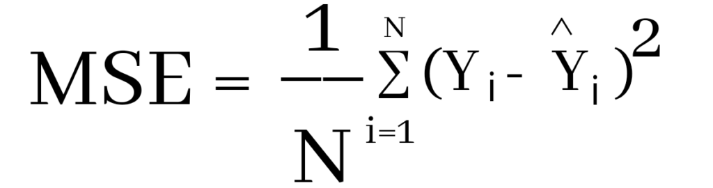
Where Yi and Ŷi represent the actual values and the predicted values, the difference between them is squared.
Derivation of Mean Squared Error
First to find the regression line for the values (1,3), (2,2), (3,6), (4,1), (5,5). The regression value for the value is y=1.6+0.4x. Next to find the new Y values. The new values for y are tabulated below.
| Given x value | Calculating y value | New y value |
|---|---|---|
| 1 | 1.6+0.4(1) | 2 |
| 2 | 1.6+0.4(2) | 2.4 |
| 3 | 1.6+0.4(3) | 2.8 |
| 4 | 1.6+0.4(4) | 3.2 |
| 5 | 1.6+0.4(5) | 3.6 |
Now to find the error ( Yi – Ŷi )
We have to square all the errors
By adding all the errors we will get the MSE
Line regression graph
Let us consider the values (1,3), (2,2), (3,6), (4,1), (5,5) to plot the graph.
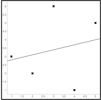
The straight line represents the predicted value in this graph, and the points represent the actual data. The difference between this line and the points is squared, known as mean squared error.
Also, Read | How to Calculate Square Root in Python
To get the Mean Squared Error in Python using NumPy
import numpy as np
true_value_of_y= [3,2,6,1,5]
predicted_value_of_y= [2.0,2.4,2.8,3.2,3.6]
MSE = np.square(np.subtract(true_value_of_y,predicted_value_of_y)).mean()
print(MSE)
Importing numpy library as np. Creating two variables. true_value_of_y holds an original value. predicted_value_of_y holds a calculated value. Next, giving the formula to calculate the mean squared error.
Output
3.6400000000000006
To get the MSE using sklearn
sklearn is a library that is used for many mathematical calculations in python. Here we are going to use this library to calculate the MSE
Syntax
sklearn.metrices.mean_squared_error(y_true, y_pred, *, sample_weight=None, multioutput='uniform_average', squared=True)
Parameters
- y_true – true value of y
- y_pred – predicted value of y
- sample_weight
- multioutput
- raw_values
- uniform_average
- squared
Returns
Mean squared error.
Code
from sklearn.metrics import mean_squared_error
true_value_of_y= [3,2,6,1,5]
predicted_value_of_y= [2.0,2.4,2.8,3.2,3.6]
mean_squared_error(true_value_of_y,predicted_value_of_y)
print(mean_squared_error(true_value_of_y,predicted_value_of_y))
From sklearn.metrices library importing mean_squared_error. Creating two variables. true_value_of_y holds an original value. predicted_value_of_y holds a calculated value. Next, giving the formula to calculate the mean squared error.
Output
3.6400000000000006
Calculating Mean Squared Error Without Using any Modules
true_value_of_y = [3,2,6,1,5]
predicted_value_of_y = [2.0,2.4,2.8,3.2,3.6]
summation_of_value = 0
n = len(true_value_of_y)
for i in range (0,n):
  difference_of_value = true_value_of_y[i] - predicted_value_of_y[i]
  squared_difference = difference_of_value**2
  summation_of_value = summation_of_value + squared_difference
MSE = summation_of_value/n
print ("The Mean Squared Error is: " , MSE)
Declaring the true values and the predicted values to two different variables. Initializing the variable summation_of_value is zero to store the values. len() function is useful to check the number of values in true_value_of_y. Creating for loop to iterate. Calculating the difference between true_value and the predicted_value. Next getting the square of the difference. Adding all the squared differences, we will get the MSE.
Output
The Mean Squared Error is: 3.6400000000000006
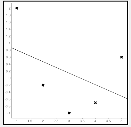
Calculate Mean Squared Error Using Negative Values
Now let us consider some negative values to calculate MSE. The values are (1,2), (3,-1), (5,0.6), (4,-0.7), (2,-0.2). The regression line equation is y=1.13-0.33x
The line regression graph for this value is:
New y values for this will be:
| Given x value | Calculating y value | New y value |
|---|---|---|
| 1 | 1.13-033(1) | 0.9 |
| 3 | 1.13-033(3) | 0.1 |
| 5 | 1.13-033(5) | -0.4 |
| 4 | 1.13-033(4) | -0.1 |
| 2 | 1.13-033(2) | 0.6 |
Code
>>> from sklearn.metrics import mean_squared_error
>>> y_true = [2,-1,0.6,-0.7,-0.2]
>>> y_pred = [0.9,0.1,-0.4,-0.1,0.6]
>>> mean_squared_error(y_true, y_pred)
First, importing a module. Declaring values to the variables. Here we are using negative value to calculate. Using the mean_squared_error module, we are calculating the MSE.
Output
0.884
Bonus: Gradient Descent
Gradient Descent is used to find the local minimum of the functions. In this case, the functions need to be differentiable. The basic idea is to move in the direction opposite from the derivate at any point.
The following code works on a set of values that are available on the Github repository.
Code:
#!/usr/bin/python
# -*- coding: utf-8 -*-
from numpy import *


def compute_error(b, m, points):
    totalError = 0
    for i in range(0, len(points)):
        x = points[i, 0]
        y = points[i, 1]
        totalError += (y - (m * x + b)) ** 2
    return totalError / float(len(points))


def gradient_step(
    b_current,
    m_current,
    points,
    learningRate,
    ):
    b_gradient = 0
    m_gradient = 0
    N = float(len(points))
    for i in range(0, len(points)):
        x = points[i, 0]
        y = points[i, 1]
        b_gradient += -(2 / N) * (y - (m_current * x + b_current))
        m_gradient += -(2 / N) * x * (y - (m_current * x + b_current))
    new_b = b_current - learningRate * b_gradient
    new_m = m_current - learningRate * m_gradient
    return [new_b, new_m]


def gradient_descent_runner(
    points,
    starting_b,
    starting_m,
    learning_rate,
    iterations,
    ):
    b = starting_b
    m = starting_m
    for i in range(iterations):
        (b, m) = gradient_step(b, m, array(points), learning_rate)
    return [b, m]


def main():
    points = genfromtxt('data.csv', delimiter=',')
    learning_rate = 0.00001
    initial_b = 0
    initial_m = 0
    iterations = 10000
    print('Starting gradient descent at b = {0}, m = {1}, error = {2}'.format(initial_b,
            initial_m, compute_error(initial_b, initial_m, points)))
    print('Running...')
    [b, m] = gradient_descent_runner(points, initial_b, initial_m,
            learning_rate, iterations)
    print('After {0} iterations b = {1}, m = {2}, error = {3}'.format(iterations,
            b, m, compute_error(b, m, points)))


if __name__ == '__main__':
    main()
Output:
Starting gradient descent at b = 0, m = 0, error = 5671.844671124282
Running...
After 10000 iterations b = 0.11558415090685024, m = 1.3769012288001614, error = 212.26220312358794
1. What is the pip command to install numpy?
pip install numpy
2. What is the pip command to install sklearn.metrices library?
pip install sklearn
3. What is the expansion of MSE?
The expansion of MSE is Mean Squared Error.
Conclusion
In this article, we have learned about the mean squared error. It is effortless to calculate. This is useful for loss function for least squares regression. The formula for the MSE is easy to memorize. We hope this article is handy and easy to understand.
What is RMSE? Also known as MSE, RMD, or RMS. What problem does it solve?
If you understand RMSE: (Root mean squared error), MSE: (Mean Squared Error) RMD (Root mean squared deviation) and RMS: (Root Mean Squared), then asking for a library to calculate this for you is unnecessary over-engineering. All these can be intuitively written in a single line of code. rmse, mse, rmd, and rms are different names for the same thing.
RMSE answers: «How similar, on average, are the numbers in list1 to list2?». The two lists must be the same size. Wash out the noise between any two given elements, wash out the size of the data collected, and get a single number result».
Intuition and ELI5 for RMSE. What problem does it solve?:
Imagine you are learning to throw darts at a dart board. Every day you practice for one hour. You want to figure out if you are getting better or getting worse. So every day you make 10 throws and measure the distance between the bullseye and where your dart hit.
You make a list of those numbers list1. Use the root mean squared error between the distances at day 1 and a list2 containing all zeros. Do the same on the 2nd and nth days. What you will get is a single number that hopefully decreases over time. When your RMSE number is zero, you hit bullseyes every time. If the rmse number goes up, you are getting worse.
Example in calculating root mean squared error in python:
import numpy as np
d = [0.000, 0.166, 0.333]   #ideal target distances, these can be all zeros.
p = [0.000, 0.254, 0.998]   #your performance goes here

print("d is: " + str(["%.8f" % elem for elem in d]))
print("p is: " + str(["%.8f" % elem for elem in p]))

def rmse(predictions, targets):
    return np.sqrt(((predictions - targets) ** 2).mean())

rmse_val = rmse(np.array(d), np.array(p))
print("rms error is: " + str(rmse_val))
Which prints:
d is: ['0.00000000', '0.16600000', '0.33300000']
p is: ['0.00000000', '0.25400000', '0.99800000']
rms error between lists d and p is: 0.387284994115
The mathematical notation:

Glyph Legend: n is a whole positive integer representing the number of throws. i represents a whole positive integer counter that enumerates sum. d stands for the ideal distances, the list2 containing all zeros in above example. p stands for performance, the list1 in the above example. superscript 2 stands for numeric squared. di is the i’th index of d. pi is the i’th index of p.
The rmse done in small steps so it can be understood:
def rmse(predictions, targets):

    differences = predictions - targets                       #the DIFFERENCEs.

    differences_squared = differences ** 2                    #the SQUAREs of ^

    mean_of_differences_squared = differences_squared.mean()  #the MEAN of ^

    rmse_val = np.sqrt(mean_of_differences_squared)           #ROOT of ^

    return rmse_val                                           #get the ^
How does every step of RMSE work:
Subtracting one number from another gives you the distance between them.
8 - 5 = 3         #absolute distance between 8 and 5 is +3
-20 - 10 = -30    #absolute distance between -20 and 10 is +30
If you multiply any number times itself, the result is always positive because negative times negative is positive:
3*3     = 9   = positive
-30*-30 = 900 = positive
Add them all up, but wait, then an array with many elements would have a larger error than a small array, so average them by the number of elements.
But we squared them all earlier, to force them positive. Undo that damage with a square root.
That leaves you with a single number that represents, on average, the distance between every value of list1 to it’s corresponding element value of list2.
If the RMSE value goes down over time we are happy because variance is decreasing. «Shrinking the Variance» here is a primitive kind of machine learning algorithm.
RMSE isn’t the most accurate line fitting strategy, total least squares is:
Root mean squared error measures the vertical distance between the point and the line, so if your data is shaped like a banana, flat near the bottom and steep near the top, then the RMSE will report greater distances to points high, but short distances to points low when in fact the distances are equivalent. This causes a skew where the line prefers to be closer to points high than low.
If this is a problem the total least squares method fixes this:
https://mubaris.com/posts/linear-regression
Gotchas that can break this RMSE function:
If there are nulls or infinity in either input list, then output rmse value is is going to not make sense. There are three strategies to deal with nulls / missing values / infinities in either list: Ignore that component, zero it out or add a best guess or a uniform random noise to all timesteps. Each remedy has its pros and cons depending on what your data means. In general ignoring any component with a missing value is preferred, but this biases the RMSE toward zero making you think performance has improved when it really hasn’t. Adding random noise on a best guess could be preferred if there are lots of missing values.
In order to guarantee relative correctness of the RMSE output, you must eliminate all nulls/infinites from the input.
RMSE has zero tolerance for outlier data points which don’t belong
Root mean squared error squares relies on all data being right and all are counted as equal. That means one stray point that’s way out in left field is going to totally ruin the whole calculation. To handle outlier data points and dismiss their tremendous influence after a certain threshold, see Robust estimators that build in a threshold for dismissal of outliers as extreme rare events that don’t need their outlandish results to change our behavior.
Hello readers. In this article, we will be focusing on Implementing RMSE – Root Mean Square Error as a metric in Python. So, let us get started!!
Before diving deep into the concept of RMSE, let us first understand the error metrics in Python.
Error metrics enable us to track the efficiency and accuracy through various metrics as shown below–
- Mean Square Error(MSE)
- Root Mean Square Error(RMSE)
- R-square
- Accuracy
- MAPE, etc.
Mean Square error is one such error metric for judging the accuracy and error rate of any machine learning algorithm for a regression problem.
So, MSE is a risk function that helps us determine the average squared difference between the predicted and the actual value of a feature or variable.
RMSE is an acronym for Root Mean Square Error, which is the square root of value obtained from Mean Square Error function.
Using RMSE, we can easily plot a difference between the estimated and actual values of a parameter of the model.
By this, we can clearly judge the efficiency of the model.
Usually, a RMSE score of less than 180 is considered a good score for a moderately or well working algorithm. In case, the RMSE value exceeds 180, we need to perform feature selection and hyper parameter tuning on the parameters of the model.
Let us now focus on the implementation of the same in the upcoming section.
Root Mean Square Error with NumPy module
Let us have a look at the below formula–
So, as seen above, Root Mean Square Error is the square root of the average of the squared differences between the estimated and the actual value of the variable/feature.
In the below example, we have implemented the concept of RMSE using the functions of NumPy module as mentioned below–
- Calculate the difference between the estimated and the actual value using
numpy.subtract()function. - Further, calculate the square of the above results using
numpy.square()function. - Finally, calculate the mean of the squared value using
numpy.mean()function. The output is the MSE score. - At the end, calculate the square root of MSE using
math.sqrt()function to get the RMSE value.
Example:
import math
y_actual = [1,2,3,4,5]
y_predicted = [1.6,2.5,2.9,3,4.1]

MSE = np.square(np.subtract(y_actual,y_predicted)).mean()

RMSE = math.sqrt(MSE)
print("Root Mean Square Error:n")
print(RMSE)
Output:
Root Mean Square Error:

0.6971370023173351
RMSE with Python scikit learn library
In this example, we have calculated the MSE score using mean_square_error() function from sklearn.metrics library.
Further, have calculated the RMSE score through the square root of MSE as shown below:
Example:
from sklearn.metrics import mean_squared_error
import math
y_actual = [1,2,3,4,5]
y_predicted = [1.6,2.5,2.9,3,4.1]

MSE = mean_squared_error(y_actual, y_predicted)

RMSE = math.sqrt(MSE)
print("Root Mean Square Error:n")
print(RMSE)
Output:
Root Mean Square Error:

0.6971370023173351
Conclusion
By this, we have come to the end of this topic. Feel free to comment below, in case you come across any question.
For more such posts related to Python, Stay tuned and till then, Happy Learning!! 🙂
Среднеквадратичная ошибка (Mean Squared Error) – Среднее арифметическое (Mean) квадратов разностей между предсказанными и реальными значениями Модели (Model) Машинного обучения (ML):

Рассчитывается с помощью формулы, которая будет пояснена в примере ниже:
$$MSE = frac{1}{n} × sum_{i=1}^n (y_i — widetilde{y}_i)^2$$
$$MSEspace{}{–}space{Среднеквадратическая}space{ошибка,}$$
$$nspace{}{–}space{количество}space{наблюдений,}$$
$$y_ispace{}{–}space{фактическая}space{координата}space{наблюдения,}$$
$$widetilde{y}_ispace{}{–}space{предсказанная}space{координата}space{наблюдения,}$$
MSE практически никогда не равен нулю, и происходит это из-за элемента случайности в данных или неучитывания Оценочной функцией (Estimator) всех факторов, которые могли бы улучшить предсказательную способность.
Пример. Исследуем линейную регрессию, изображенную на графике выше, и установим величину среднеквадратической Ошибки (Error). Фактические координаты точек-Наблюдений (Observation) выглядят следующим образом:

Мы имеем дело с Линейной регрессией (Linear Regression), потому уравнение, предсказывающее положение записей, можно представить с помощью формулы:
$$y = M * x + b$$
$$yspace{–}space{значение}space{координаты}space{оси}space{y,}$$
$$Mspace{–}space{уклон}space{прямой}$$
$$xspace{–}space{значение}space{координаты}space{оси}space{x,}$$
$$bspace{–}space{смещение}space{прямой}space{относительно}space{начала}space{координат}$$
Параметры M и b уравнения нам, к счастью, известны в данном обучающем примере, и потому уравнение выглядит следующим образом:
$$y = 0,5252 * x + 17,306$$
Зная координаты реальных записей и уравнение линейной регрессии, мы можем восстановить полные координаты предсказанных наблюдений, обозначенных серыми точками на графике выше. Простой подстановкой значения координаты x в уравнение мы рассчитаем значение координаты ỹ:

Рассчитаем квадрат разницы между Y и Ỹ:

Сумма таких квадратов равна 4 445. Осталось только разделить это число на количество наблюдений (9):
$$MSE = frac{1}{9} × 4445 = 493$$
Само по себе число в такой ситуации становится показательным, когда Дата-сайентист (Data Scientist) предпринимает попытки улучшить предсказательную способность модели и сравнивает MSE каждой итерации, выбирая такое уравнение, что сгенерирует наименьшую погрешность в предсказаниях.
MSE и Scikit-learn
Среднеквадратическую ошибку можно вычислить с помощью SkLearn. Для начала импортируем функцию:
import sklearn
from sklearn.metrics import mean_squared_error
Инициализируем крошечные списки, содержащие реальные и предсказанные координаты y:
y_true = [5, 41, 70, 77, 134, 68, 138, 101, 131]
y_pred = [23, 35, 55, 90, 93, 103, 118, 121, 129]
Инициируем функцию mean_squared_error(), которая рассчитает MSE тем же способом, что и формула выше:
mean_squared_error(y_true, y_pred)
Интересно, что конечный результат на 3 отличается от расчетов с помощью Apple Numbers:
496.0Ноутбук, не требующий дополнительной настройки на момент написания статьи, можно скачать здесь.
Автор оригинальной статьи: @mmoshikoo
Фото: @tobyelliott