Main Content
Syntax
Description
example
err = immse(X,Y)
calculates the mean-squared error (MSE) between the arrays X
and Y. A lower MSE value indicates greater similarity between
X and Y.
Examples
collapse all
Calculate Mean-Squared Error in Noisy Image
Read image and display it.
ref = imread('pout.tif');
imshow(ref)
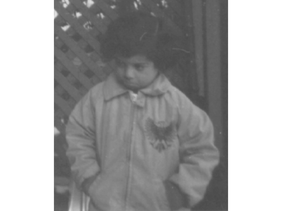
Create another image by adding noise to a copy of the reference image.
A = imnoise(ref,'salt & pepper', 0.02);
imshow(A)
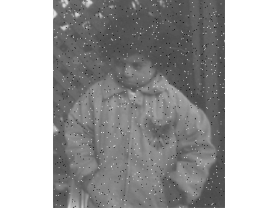
Calculate mean-squared error between the two images.
err = immse(A, ref);
fprintf('n The mean-squared error is %0.4fn', err);
The mean-squared error is 353.7631
Input Arguments
collapse all
X — Input array
numeric array
Input array, specified as a numeric array of any dimension.
Data Types: single | double | int8 | int16 | int32 | uint8 | uint16 | uint32
Y — Input array
numeric array
Input array, specified as a numeric array of the same size and data type as
X.
Data Types: single | double | int8 | int16 | int32 | uint8 | uint16 | uint32
Output Arguments
collapse all
err — Mean-squared error
positive number
Mean-squared error, returned as a positive number. The data type of err
is double unless the input arguments are of data type
single, in which case err is of
data type single
Data Types: single | double
Extended Capabilities
C/C++ Code Generation
Generate C and C++ code using MATLAB® Coder™.
immse supports the generation of C
code (requires MATLAB®
Coder™). For more information, see Code Generation for Image Processing.
GPU Code Generation
Generate CUDA® code for NVIDIA® GPUs using GPU Coder™.
Version History
Introduced in R2014b
Root-mean-square error between arrays
Syntax
Description
example
E = rmse(F,A)
returns the root-mean-square
error (RMSE) between the forecast (predicted) array F and the
actual (observed) array A.
-
FandAmust either be the same size or
have sizes that are compatible. -
If
FandAare vectors of the same size,
thenEis a scalar. -
If
F-Ais a matrix, thenEis a row vector
containing the RMSE for each column. -
If
FandAare multidimensional arrays,
thenEcontains the RMSE computed along the first array dimension
of size greater than 1, with elements treated as vectors. The size of
Ein this dimension is 1, while the sizes of all other
dimensions are the same as inF-A.
E = rmse(F,A,"all")
returns the RMSE of all elements in F and A.
example
E = rmse(F,A,dim)
operates along the dimension dim. For example, if F
and A are matrices, then rmse(F,A,2) operates on the
elements in each row and returns a column vector containing the RMSE of each row.
example
E = rmse(F,A,vecdim)
operates along the dimensions specified in the vector vecdim. For
example, if F and A are matrices, then
rmse(F,A,[1 2]) operates on all the elements in F
and A because every element of a matrix is contained in the array slice
defined by dimensions 1 and 2.
example
E = rmse(___,nanflag)
specifies whether to include or omit NaN values in the calculation.
Specify nanflag after all other input arguments from the previous
syntaxes. For example, rmse(F,A,"includenan") includes the
NaN values in the calculation, while
rmse(F,A,"omitnan") ignores them.
example
E = rmse(___,Weight=W)
specifies a weighting scheme W and returns the weighted RMSE. If
W is a vector, its length must equal the length of the operating
dimension. If W is a matrix or multidimensional array, it must have the
same dimensions as F, A, or F-A.
You cannot specify a weighting scheme if you specify vecdim or
"all".
Examples
collapse all
RMSE of Two Forecasts
Create two column vectors of forecast (predicted) data and one column vector of actual (observed) data.
F1 = [1; 10; 9];
F2 = [2; 5; 10];
A = [1; 9; 10];
Compute the RMSE between each forecast and the actual data.
Alternatively, create a matrix containing both forecasts and compute the RMSE between each forecast and the actual data in one command.
The first element of E is the RMSE between the first forecast column and the actual data. The second element of E is the RMSE between the second forecast column and the actual data.
RMSE of Matrix Rows
Create a matrix of forecast data and a matrix of actual data.
F = [17 19; 1 6; 16 15];
A = [17 25; 3 4; 16 13];
Compute the RMSE between the forecast and the actual data across each row by specifying the operating dimension as 2. The smallest RMSE corresponds to the RMSE between the third rows of the forecast data and actual data.
E = 3×1

    4.2426
    2.0000
    1.4142
RMSE of Array Pages
Create a 3-D array with pages containing forecast data and a matrix of actual data.
F(:,:,1) = [2 4; -2 1];
F(:,:,2) = [4 4; 8 -3];
A = [6 7; 1 4];
Compute the RMSE between the predicted data in each page of the forecast array and the actual data matrix by specifying a vector of operating dimensions 1 and 2.
E =
E(:,:,1) =

    3.2787


E(:,:,2) =

    5.2678
The first page of E contains the RMSE between the first page of F and the matrix A. The second page of E contains the RMSE between the second page of F and the matrix A.
RMSE Excluding NaN
Create a row vector of forecast data and a row vector of actual data containing a missing value.
F = [1 6 10 5];
A = [2 6 NaN 3];
Compute the RMSE between the forecast and the actual data.
Because NaN values are included in the RMSE calculation by default, the result is NaN. Ignore the missing value in the input data by specifying "omitnan". Now, the function computes the RMSE for only the first, second, and fourth columns of the input data.
Eomit = rmse(F,A,"omitnan")
Specify RMSE Weight Vector
Create a forecast column vector and an actual column vector.
F = [2; 10; 13];
A = [1; 9; 10];
Compute the RMSE between the forecast and actual data according to a weighting scheme specified by W.
W = [0.5; 0.25; 0.25];
E = rmse(F,A,Weight=W)
Input Arguments
collapse all
F — Forecast array
vector | matrix | multidimensional array
Forecast or predicted array, specified as a vector, matrix, or multidimensional
array.
Inputs F and A must either be the same size or
have sizes that are compatible. For example, F is an
m-by-n matrix and
A is a 1-by-n row vector. For more
information, see Compatible Array Sizes for Basic Operations.
Data Types: single | double
Complex Number Support: Yes
A — Actual array
vector | matrix | multidimensional array
Actual or observed array, specified as a vector, matrix, or multidimensional
array.
Inputs F and A must either be the same size or
have sizes that are compatible. For example, F is an
m-by-n matrix and
A is a 1-by-n row vector. For more
information, see Compatible Array Sizes for Basic Operations.
Data Types: single | double
Complex Number Support: Yes
dim — Dimension to operate along
positive integer scalar
Dimension
to operate along, specified as a positive integer scalar. If you do not specify the dimension,
then the default is the first array dimension of size greater than 1.
The size of E in the operating dimension is 1. All other
dimensions of E have the same size as the result of
F-A.
For example, consider four forecasts in a 3-by-4 matrix, F, and
actual data in a 3-by-1 column vector, A:
-
rmse(F,A,1)computes the RMSE of the elements in each
column and returns a 1-by-4 row vector.The size of
Ein the operating dimension is 1. The
difference ofFandAis a 3-by-4 matrix.
The size ofEin the nonoperating dimension is the same as the
second dimension ofF-A, which is 4. The overall size of
Ebecomes 1-by-4. -
rmse(F,A,2)computes the RMSE of the elements in each row
and returns a 3-by-1 column vector.The size of
Ein the operating dimension is 1. The
difference ofFandAis a 3-by-4 matrix.
The size ofEin the nonoperating dimension is the same as the
first dimension ofF-A, which is 3. The overall size of
Ebecomes 3-by-1.
vecdim — Vector of dimensions to operate along
vector of positive integers
Vector of dimensions to operate along, specified as a vector of positive integers.
Each element represents a dimension of the input arrays. The size of
E in the operating dimensions is 1. All other dimensions of
E have the same size as the result of
F-A.
For example, consider forecasts in a 2-by-3-by-3 array, F, and
actual data in a 1-by-3 row vector, A:
-
rmse(F,A,[1 2])computes the RMSE over each page of
Fand returns a 1-by-1-by-3 array.The size of
Ein the operating dimensions is 1. The
difference ofFandAis a 2-by-3-by-3
array. The size ofEin the nonoperating dimension is the same
as the third dimension ofF-A, which is 3. The overall size of
Ebecomes 1-by-1-by-3.
nanflag — NaN condition
"includenan" (default) | "omitnan"
NaN condition, specified as one of these values:
-
"includenan"— IncludeNaNvalues
when computing the RMSE. If any elements inFor
AareNaN, then the result is
NaN. -
"omitnan"— Ignore allNaNvalues
in the input. If all elements inF,A, or
WareNaN, then the result is
NaN.
W — Weighting scheme
vector | matrix | multidimensional array
Weighting scheme, specified as a vector, matrix, or multidimensional array. The
elements of W must be nonnegative.
If W is a vector, it must have the same length as the operating
dimension. If W is a matrix or multidimensional array, it must have
the same dimensions as F, A, or
F-A.
You cannot specify this argument if you specify vecdim or
"all".
Data Types: single | double
Output Arguments
collapse all
E — Root-mean-square error
scalar | vector | matrix | multidimensional array
Root-mean-square error, returned as a scalar, vector, matrix, or multidimensional
array. The default size of E is as follows.
-
If
FandAare vectors of the same size,
thenEis a scalar. -
If
F-Ais a matrix, thenEis a row vector
containing the RMSE for each column. -
If
FandAare multidimensional arrays,
thenEcontains the RMSE computed along the first array dimension
of size greater than 1, with elements treated as vectors. The size of
Ein this dimension is 1, while the sizes of all other
dimensions are the same as inF-A.
More About
collapse all
Root-Mean-Square Error
For a forecast array F and actual array
A made up of n scalar observations, the
root-mean-square error is defined as
with the summation performed along the specified dimension.
Weighted Root-Mean-Square Error
For a forecast array F and actual array
A made up of n scalar observations and weighting
scheme W, the weighted root-mean-square error is defined as
with the summation performed along the specified dimension.
Extended Capabilities
GPU Arrays
Accelerate code by running on a graphics processing unit (GPU) using Parallel Computing Toolbox™.
This function fully supports GPU arrays. For more information, see Run MATLAB Functions on a GPU (Parallel Computing Toolbox).
Distributed Arrays
Partition large arrays across the combined memory of your cluster using Parallel Computing Toolbox™.
This function fully supports distributed arrays. For more
information, see Run MATLAB Functions with Distributed Arrays (Parallel Computing Toolbox).
Version History
Introduced in R2022b
msesim
Estimated mean squared error for adaptive filters
Syntax
Description
example
mse = msesim(adaptFilt,x,d)
estimates the mean squared error of the adaptive filter at each time instant given
the input and the desired response signal sequences in x and
d.
example
[mse,meanw,w,tracek] = msesim(adaptFilt,x,d)
also calculates the sequences of coefficient vector means,
meanw, adaptive filter coefficients,
w, and the total coefficient error powers,
tracek, corresponding to the simulated behavior of the
adaptive filter.
example
[___] = msesim(adaptFilt,x,m)
specifies an optional decimation factor for computing mse,
meanw, and tracek. If
m > 1, every mth value of each of
these sequences is saved. If omitted, the value of m defaults
to 1.
Examples
collapse all
Predict Mean Squared Error for LMS Filter
The mean squared error (MSE) measures the average of the squares of the errors between the desired signal and the primary signal input to the adaptive filter. Reducing this error converges the primary input to the desired signal. Determine the predicted value of MSE and the simulated value of MSE at each time instant using the msepred and msesim functions. Compare these MSE values with each other and with respect to the minimum MSE and steady-state MSE values. In addition, compute the sum of the squares of the coefficient errors given by the trace of the coefficient covariance matrix.
Note: If you are using R2016a or an earlier release, replace each call to the object with the equivalent step syntax. For example, obj(x) becomes step(obj,x).
Initialization
Create a dsp.FIRFilter System object™ that represents the unknown system. Pass the signal, x, to the FIR filter. The output of the unknown system is the desired signal, d, which is the sum of the output of the unknown system (FIR filter) and an additive noise signal, n.
num = fir1(31,0.5);
fir = dsp.FIRFilter('Numerator',num);
iir = dsp.IIRFilter('Numerator',sqrt(0.75),...
        'Denominator',[1 -0.5]);
x = iir(sign(randn(2000,25)));
n = 0.1*randn(size(x));
d = fir(x) + n;
LMS Filter
Create a dsp.LMSFilter System object to create a filter that adapts to output the desired signal. Set the length of the adaptive filter to 32 taps, step size to 0.008, and the decimation factor for analysis and simulation to 5. The variable simmse represents the simulated MSE between the output of the unknown system, d, and the output of the adaptive filter. The variable mse gives the corresponding predicted value.
l = 32;
mu = 0.008;
m  = 5;

lms = dsp.LMSFilter('Length',l,'StepSize',mu);
[mmse,emse,meanW,mse,traceK] = msepred(lms,x,d,m);
[simmse,meanWsim,Wsim,traceKsim] = msesim(lms,x,d,m);
Plot the MSE Results
Compare the values of simulated MSE, predicted MSE, minimum MSE, and the final MSE. The final MSE value is given by the sum of minimum MSE and excess MSE.
nn = m:m:size(x,1);
semilogy(nn,simmse,[0 size(x,1)],[(emse+mmse)...
    (emse+mmse)],nn,mse,[0 size(x,1)],[mmse mmse])
title('Mean Squared Error Performance')
axis([0 size(x,1) 0.001 10])
legend('MSE (Sim.)','Final MSE','MSE','Min. MSE')
xlabel('Time Index')
ylabel('Squared Error Value')
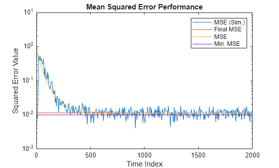
The predicted MSE follows the same trajectory as the simulated MSE. Both these trajectories converge with the steady-state (final) MSE.
Plot the Coefficient Trajectories
meanWsim is the mean value of the simulated coefficients given by msesim. meanW is the mean value of the predicted coefficients given by msepred.
Compare the simulated and predicted mean values of LMS filter coefficients 12,13,14, and 15.
plot(nn,meanWsim(:,12),'b',nn,meanW(:,12),'r',nn,...
meanWsim(:,13:15),'b',nn,meanW(:,13:15),'r')
PlotTitle ={'Average Coefficient Trajectories for';...
            'W(12), W(13), W(14), and W(15)'}
PlotTitle = 2x1 cell
    {'Average Coefficient Trajectories for'}
    {'W(12), W(13), W(14), and W(15)'      }
title(PlotTitle)
legend('Simulation','Theory')
xlabel('Time Index')
ylabel('Coefficient Value')
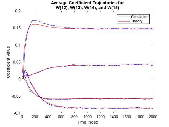
In steady state, both the trajectories converge.
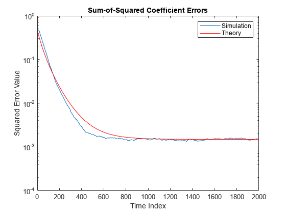
Sum of Squared Coefficient Errors
Compare the sum of the squared coefficient errors given by msepred and msesim. These values are given by the trace of the coefficient covariance matrix.
semilogy(nn,traceKsim,nn,traceK,'r')
title('Sum-of-Squared Coefficient Errors')
axis([0 size(x,1) 0.0001 1])
legend('Simulation','Theory')
xlabel('Time Index')
ylabel('Squared Error Value')
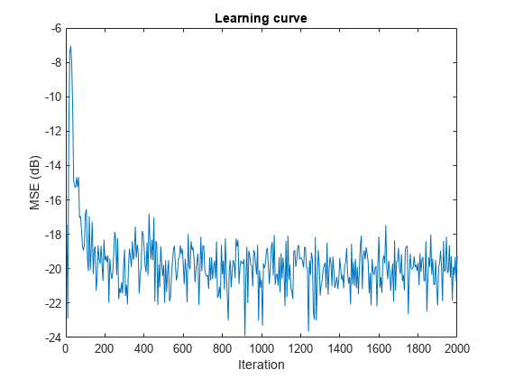
System Identification of FIR Filter Using Filtered XLMS Filter
Identify an unknown system by performing active noise control using a filtered-x LMS algorithm. The objective of the adaptive filter is to minimize the error signal between the output of the adaptive filter and the output of the unknown system (or the system to be identified). Once the error signal is minimal, the unknown system converges to the adaptive filter.
Note: If you are using R2016a or an earlier release, replace each call to the object with the equivalent step syntax. For example, obj(x) becomes step(obj,x).
Initialization
Create a dsp.FIRFilter System object that represents the system to be identified. Pass the signal, x, to the FIR filter. The output of the unknown system is the desired signal, d, which is the sum of the output of the unknown system (FIR filter) and an additive noise signal, n.
num = fir1(31,0.5);
fir = dsp.FIRFilter('Numerator',num);
iir = dsp.IIRFilter('Numerator',sqrt(0.75),...
        'Denominator',[1 -0.5]);
x = iir(sign(randn(2000,25)));
n = 0.1*randn(size(x));
d = fir(x) + n;
Adaptive Filter
Create a dsp.FilteredXLMSFilter System object to create an adaptive filter that uses the filtered-x LMS algorithm. Set the length of the adaptive filter to 32 taps, step size to 0.008, and the decimation factor for analysis and simulation to 5. The variable simmse represents the error between the output of the unknown system, d, and the output of the adaptive filter.
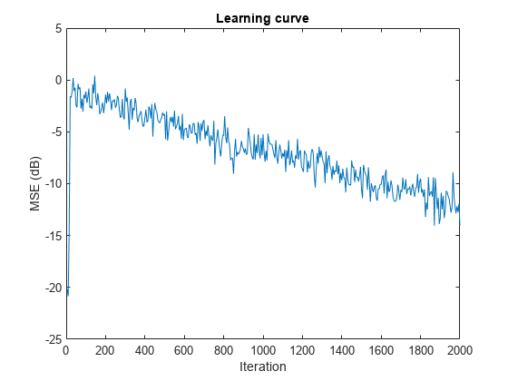
l = 32;
mu = 0.008;
m  = 5;
fxlms = dsp.FilteredXLMSFilter(l,'StepSize',mu);
[simmse,meanWsim,Wsim,traceKsim] = msesim(fxlms,x,d,m);
plot(m*(1:length(simmse)),10*log10(simmse))
xlabel('Iteration')
ylabel('MSE (dB)')
% Plot the learning curve for filtered-x LMS filter
% used in system identification
title('Learning curve')
With each iteration of adaptation, the value of simmse decreases to a minimal value, indicating that the unknown system has converged to the adaptive filter.
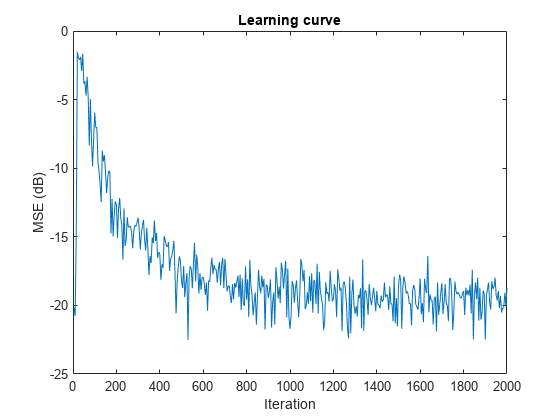
System Identification of FIR Filter Using Adaptive Lattice Filter
Note: If you are using R2016a or an earlier release, replace each call to the object with the equivalent step syntax. For example, obj(x) becomes step(obj,x).
ha = fir1(31,0.5);
% FIR system to be identified
fir = dsp.FIRFilter('Numerator',ha);
iir = dsp.IIRFilter('Numerator',sqrt(0.75),...
        'Denominator',[1 -0.5]);
x = iir(sign(randn(2000,25)));
% Observation noise signal
n = 0.1*randn(size(x));
 % Desired signal
d = fir(x)+n;
% Filter length
l = 32;
% Decimation factor for analysis
% and simulation results
m  = 5;
ha = dsp.AdaptiveLatticeFilter(l);
[simmse,meanWsim,Wsim,traceKsim] = msesim(ha,x,d,m);
plot(m*(1:length(simmse)),10*log10(simmse));
xlabel('Iteration');
ylabel('MSE (dB)');
% Plot the learning curve used for
% adaptive lattice filter used in system identification
title('Learning curve')
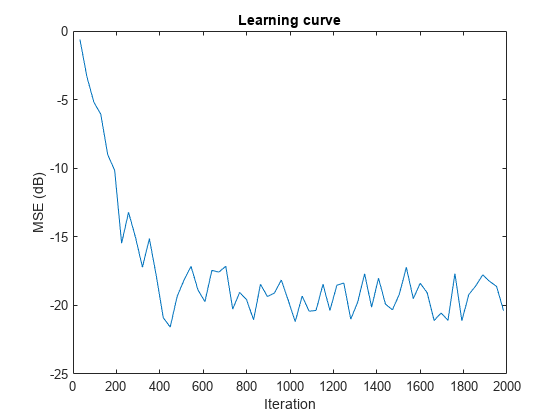
System Identification of FIR Filter Using Block LMS Filter
Note: If you are using R2016a or an earlier release, replace each call to the object with the equivalent step syntax. For example, obj(x) becomes step(obj,x).
fir = fir1(31,0.5);
% FIR system to be identified
firFilter = dsp.FIRFilter('Numerator',fir);
iirFilter = dsp.IIRFilter('Numerator',sqrt(0.75),...
        'Denominator',[1 -0.5]);
x = iirFilter(sign(randn(2000,25)));
% Observation noise signal
n = 0.1*randn(size(x));
% Desired signal
d = firFilter(x)+n;
% Filter length
l = 32;
% Block LMS Step size
mu = 0.008;
% Decimation factor for analysis
% and simulation results
m  = 32;
fir = dsp.BlockLMSFilter(l,'StepSize',mu);
[simmse,meanWsim,Wsim,traceKsim] = msesim(fir,x,d,m);
plot(m*(1:length(simmse)),10*log10(simmse));
xlabel('Iteration'); ylabel('MSE (dB)');
% Plot the learning curve for
% block LMS filter used in system identification
title('Learning curve')
System Identification of FIR Filter Using Affine Projection Filter
Note: If you are using R2016a or an earlier release, replace each call to the object with the equivalent step syntax. For example, obj(x) becomes step(obj,x).
ha = fir1(31,0.5);
% FIR system to be identified
fir = dsp.FIRFilter('Numerator',ha);
iir = dsp.IIRFilter('Numerator',sqrt(0.75),...
        'Denominator',[1 -0.5]);
x = iir(sign(randn(2000,25)));
% Observation noise signal
n = 0.1*randn(size(x));
% Desired signal
d = fir(x)+n;
% Filter length
l = 32;
% Affine Projection filter Step size.
mu = 0.008;
% Decimation factor for analysis
% and simulation results
m  = 5;

apf = dsp.AffineProjectionFilter(l,'StepSize',mu);
[simmse,meanWsim,Wsim,traceKsim] = msesim(apf,x,d,m);
plot(m*(1:length(simmse)),10*log10(simmse));
xlabel('Iteration'); ylabel('MSE (dB)');
% Plot the learning curve for affine projection filter
% used in system identification
title('Learning curve')
Input Arguments
collapse all
adaptFilt — Adaptive filter System object™
adaptive filter System object
x — Input signal
scalar | column vector | matrix
Input signal, specified as a scalar, column vector, or matrix. Columns of
the matrix x contain individual input signal sequences.
The input, x, and the desired signal,
d, must have the same size and data type.
If adaptFilt is a dsp.BlockLMSFilter object, the
input signal frame size must be greater than or equal to the value you
specify in the BlockSize property of the object.
Data Types: single | double
d — Desired signal
scalar | column vector | matrix
Desired response signal, specified as a scalar, column vector, or matrix.
Columns of the matrix d contain individual desired
signal sequences. The input, x, and the desired signal,
d, must have the same size and the data
type.
If adaptFilt is a dsp.BlockLMSFilter
System object, the desired signal frame size must be greater than or equal
to the value you specify in the BlockSize property of
the object.
Data Types: single | double
m — Decimation factor
1 (default) | positive scalar
Decimation factor, specified as a positive scalar. Every
mth value of the estimated sequences is saved into
the corresponding output arguments, mse,
meanw, w, and
tracek. If m equals 1, every
value of these sequences is saved.
If adaptFilt is a dsp.BlockLMSFilter
System object, the decimation factor must be a multiple of the value you
specify in the BlockSize property of the object.
Data Types: single | double | int8 | int16 | int32 | int64 | uint8 | uint16 | uint32 | uint64 | logical
Output Arguments
collapse all
mse — Sequence of mean squared errors
column vector
Estimates of the mean squared error of the adaptive filter at each time
instant, returned as a column vector.
If the adaptive filter is dsp.BlockLMSFilter and the
decimation factor m is specified, length of
mse equals floor(M/m).
M is the frame size (number of rows) of the input
signal, x. If m is not specified,
the length of mse equals floor(M/B),
where B is the value you specify in the
BlockSize property of the object. The input signal
frame size must be greater than or equal to the value you specify in the
BlockSize property of the object. The decimation
factor, if specified, must be a multiple of the
BlockSize property.
For the other adaptive filters, if the decimation factor,
m = 1, the length of mse
equals the frame size of the input signal. If m > 1,
the length of mse equals
floor(M/m).
Data Types: double
meanw — Sequence of coefficient vector means
matrix
Sequence of coefficient vector means of the adaptive filter at each time
instant, estimated as a matrix. The columns of this matrix contain estimates
of the mean values of the adaptive filter coefficients at each time
instant.
If the adaptive filter is dsp.BlockLMSFilter and the
decimation factor m is specified, the dimensions of
meanw is
floor(M/m)-by-N.
M is the frame size (number of rows) of the input
signal, x. N is the length of the
filter weights vector, specified by the Length property
of the adaptive filter. If m is not specified, the
dimensions of meanw is
floor(M/B)-by-N, where
B is the value you specify in the
BlockSize property of the object. The input signal
frame size must be greater than or equal to the value you specify in the
BlockSize property of the object. The decimation
factor, if specified, must be a multiple of the
BlockSize property.
For the other adaptive filters, If the decimation factor,
m = 1, the dimensions of meanw
is M-by-N. If m >
1, the dimensions of meanw is
floor(M/m)-by-N.
Data Types: double
w — Final values of adaptive filter coefficients
row vector
Final values of the adaptive filter coefficients for the algorithm
corresponding to adaptFilt, returned as a row vector. The
length of the row vector equals the value you specify in the
Length property of the object.
Data Types: single | double
tracek — Sequence of total coefficient error powers
column vector
Sequence of total coefficient error powers, estimated as a column vector.
This column vector contains estimates of the total coefficient error power
of the adaptive filter at each time instant.
If the adaptive filter is dsp.BlockLMSFilter and the
decimation factor m is specified, length of
tracek equals floor(M/m).
M is the frame size (number of rows) of the input
signal, x. If m is not specified,
the length of tracek equals
floor(M/B), where B is the value
you specify in the BlockSize property of the object.
The input signal frame size must be greater than or equal to the value you
specify in the BlockSize property of the object. The
decimation factor, if specified, must be a multiple of the
BlockSize property.
For the other adaptive filters, if the decimation factor,
m = 1, the length of tracek
equals the frame size of the input signal. If m > 1,
the length of tracek equals
floor(M/m).
Data Types: double
References
[1] Hayes, M.H. Statistical Digital Signal Processing and
Modeling. New York: John Wiley & Sons, 1996.
Version History
Introduced in R2012a
msesim
Estimated mean squared error for adaptive filters
Syntax
Description
example
mse = msesim(adaptFilt,x,d)
estimates the mean squared error of the adaptive filter at each time instant given
the input and the desired response signal sequences in x and
d.
example
[mse,meanw,w,tracek] = msesim(adaptFilt,x,d)
also calculates the sequences of coefficient vector means,
meanw, adaptive filter coefficients,
w, and the total coefficient error powers,
tracek, corresponding to the simulated behavior of the
adaptive filter.
example
[___] = msesim(adaptFilt,x,m)
specifies an optional decimation factor for computing mse,
meanw, and tracek. If
m > 1, every mth value of each of
these sequences is saved. If omitted, the value of m defaults
to 1.
Examples
collapse all
Predict Mean Squared Error for LMS Filter
The mean squared error (MSE) measures the average of the squares of the errors between the desired signal and the primary signal input to the adaptive filter. Reducing this error converges the primary input to the desired signal. Determine the predicted value of MSE and the simulated value of MSE at each time instant using the msepred and msesim functions. Compare these MSE values with each other and with respect to the minimum MSE and steady-state MSE values. In addition, compute the sum of the squares of the coefficient errors given by the trace of the coefficient covariance matrix.
Note: If you are using R2016a or an earlier release, replace each call to the object with the equivalent step syntax. For example, obj(x) becomes step(obj,x).
Initialization
Create a dsp.FIRFilter System object™ that represents the unknown system. Pass the signal, x, to the FIR filter. The output of the unknown system is the desired signal, d, which is the sum of the output of the unknown system (FIR filter) and an additive noise signal, n.
num = fir1(31,0.5);
fir = dsp.FIRFilter('Numerator',num);
iir = dsp.IIRFilter('Numerator',sqrt(0.75),...
        'Denominator',[1 -0.5]);
x = iir(sign(randn(2000,25)));
n = 0.1*randn(size(x));
d = fir(x) + n;
LMS Filter
Create a dsp.LMSFilter System object to create a filter that adapts to output the desired signal. Set the length of the adaptive filter to 32 taps, step size to 0.008, and the decimation factor for analysis and simulation to 5. The variable simmse represents the simulated MSE between the output of the unknown system, d, and the output of the adaptive filter. The variable mse gives the corresponding predicted value.
l = 32;
mu = 0.008;
m  = 5;

lms = dsp.LMSFilter('Length',l,'StepSize',mu);
[mmse,emse,meanW,mse,traceK] = msepred(lms,x,d,m);
[simmse,meanWsim,Wsim,traceKsim] = msesim(lms,x,d,m);
Plot the MSE Results
Compare the values of simulated MSE, predicted MSE, minimum MSE, and the final MSE. The final MSE value is given by the sum of minimum MSE and excess MSE.
nn = m:m:size(x,1);
semilogy(nn,simmse,[0 size(x,1)],[(emse+mmse)...
    (emse+mmse)],nn,mse,[0 size(x,1)],[mmse mmse])
title('Mean Squared Error Performance')
axis([0 size(x,1) 0.001 10])
legend('MSE (Sim.)','Final MSE','MSE','Min. MSE')
xlabel('Time Index')
ylabel('Squared Error Value')
The predicted MSE follows the same trajectory as the simulated MSE. Both these trajectories converge with the steady-state (final) MSE.
Plot the Coefficient Trajectories
meanWsim is the mean value of the simulated coefficients given by msesim. meanW is the mean value of the predicted coefficients given by msepred.
Compare the simulated and predicted mean values of LMS filter coefficients 12,13,14, and 15.
plot(nn,meanWsim(:,12),'b',nn,meanW(:,12),'r',nn,...
meanWsim(:,13:15),'b',nn,meanW(:,13:15),'r')
PlotTitle ={'Average Coefficient Trajectories for';...
            'W(12), W(13), W(14), and W(15)'}
PlotTitle = 2x1 cell
    {'Average Coefficient Trajectories for'}
    {'W(12), W(13), W(14), and W(15)'      }
title(PlotTitle)
legend('Simulation','Theory')
xlabel('Time Index')
ylabel('Coefficient Value')
In steady state, both the trajectories converge.
Sum of Squared Coefficient Errors
Compare the sum of the squared coefficient errors given by msepred and msesim. These values are given by the trace of the coefficient covariance matrix.
semilogy(nn,traceKsim,nn,traceK,'r')
title('Sum-of-Squared Coefficient Errors')
axis([0 size(x,1) 0.0001 1])
legend('Simulation','Theory')
xlabel('Time Index')
ylabel('Squared Error Value')
System Identification of FIR Filter Using Filtered XLMS Filter
Identify an unknown system by performing active noise control using a filtered-x LMS algorithm. The objective of the adaptive filter is to minimize the error signal between the output of the adaptive filter and the output of the unknown system (or the system to be identified). Once the error signal is minimal, the unknown system converges to the adaptive filter.
Note: If you are using R2016a or an earlier release, replace each call to the object with the equivalent step syntax. For example, obj(x) becomes step(obj,x).
Initialization
Create a dsp.FIRFilter System object that represents the system to be identified. Pass the signal, x, to the FIR filter. The output of the unknown system is the desired signal, d, which is the sum of the output of the unknown system (FIR filter) and an additive noise signal, n.
num = fir1(31,0.5);
fir = dsp.FIRFilter('Numerator',num);
iir = dsp.IIRFilter('Numerator',sqrt(0.75),...
        'Denominator',[1 -0.5]);
x = iir(sign(randn(2000,25)));
n = 0.1*randn(size(x));
d = fir(x) + n;
Adaptive Filter
Create a dsp.FilteredXLMSFilter System object to create an adaptive filter that uses the filtered-x LMS algorithm. Set the length of the adaptive filter to 32 taps, step size to 0.008, and the decimation factor for analysis and simulation to 5. The variable simmse represents the error between the output of the unknown system, d, and the output of the adaptive filter.
l = 32;
mu = 0.008;
m  = 5;
fxlms = dsp.FilteredXLMSFilter(l,'StepSize',mu);
[simmse,meanWsim,Wsim,traceKsim] = msesim(fxlms,x,d,m);
plot(m*(1:length(simmse)),10*log10(simmse))
xlabel('Iteration')
ylabel('MSE (dB)')
% Plot the learning curve for filtered-x LMS filter
% used in system identification
title('Learning curve')
With each iteration of adaptation, the value of simmse decreases to a minimal value, indicating that the unknown system has converged to the adaptive filter.
System Identification of FIR Filter Using Adaptive Lattice Filter
Note: If you are using R2016a or an earlier release, replace each call to the object with the equivalent step syntax. For example, obj(x) becomes step(obj,x).
ha = fir1(31,0.5);
% FIR system to be identified
fir = dsp.FIRFilter('Numerator',ha);
iir = dsp.IIRFilter('Numerator',sqrt(0.75),...
        'Denominator',[1 -0.5]);
x = iir(sign(randn(2000,25)));
% Observation noise signal
n = 0.1*randn(size(x));
 % Desired signal
d = fir(x)+n;
% Filter length
l = 32;
% Decimation factor for analysis
% and simulation results
m  = 5;
ha = dsp.AdaptiveLatticeFilter(l);
[simmse,meanWsim,Wsim,traceKsim] = msesim(ha,x,d,m);
plot(m*(1:length(simmse)),10*log10(simmse));
xlabel('Iteration');
ylabel('MSE (dB)');
% Plot the learning curve used for
% adaptive lattice filter used in system identification
title('Learning curve')
System Identification of FIR Filter Using Block LMS Filter
Note: If you are using R2016a or an earlier release, replace each call to the object with the equivalent step syntax. For example, obj(x) becomes step(obj,x).
fir = fir1(31,0.5);
% FIR system to be identified
firFilter = dsp.FIRFilter('Numerator',fir);
iirFilter = dsp.IIRFilter('Numerator',sqrt(0.75),...
        'Denominator',[1 -0.5]);
x = iirFilter(sign(randn(2000,25)));
% Observation noise signal
n = 0.1*randn(size(x));
% Desired signal
d = firFilter(x)+n;
% Filter length
l = 32;
% Block LMS Step size
mu = 0.008;
% Decimation factor for analysis
% and simulation results
m  = 32;
fir = dsp.BlockLMSFilter(l,'StepSize',mu);
[simmse,meanWsim,Wsim,traceKsim] = msesim(fir,x,d,m);
plot(m*(1:length(simmse)),10*log10(simmse));
xlabel('Iteration'); ylabel('MSE (dB)');
% Plot the learning curve for
% block LMS filter used in system identification
title('Learning curve')
System Identification of FIR Filter Using Affine Projection Filter
Note: If you are using R2016a or an earlier release, replace each call to the object with the equivalent step syntax. For example, obj(x) becomes step(obj,x).
ha = fir1(31,0.5);
% FIR system to be identified
fir = dsp.FIRFilter('Numerator',ha);
iir = dsp.IIRFilter('Numerator',sqrt(0.75),...
        'Denominator',[1 -0.5]);
x = iir(sign(randn(2000,25)));
% Observation noise signal
n = 0.1*randn(size(x));
% Desired signal
d = fir(x)+n;
% Filter length
l = 32;
% Affine Projection filter Step size.
mu = 0.008;
% Decimation factor for analysis
% and simulation results
m  = 5;

apf = dsp.AffineProjectionFilter(l,'StepSize',mu);
[simmse,meanWsim,Wsim,traceKsim] = msesim(apf,x,d,m);
plot(m*(1:length(simmse)),10*log10(simmse));
xlabel('Iteration'); ylabel('MSE (dB)');
% Plot the learning curve for affine projection filter
% used in system identification
title('Learning curve')
Input Arguments
collapse all
adaptFilt — Adaptive filter System object™
adaptive filter System object
x — Input signal
scalar | column vector | matrix
Input signal, specified as a scalar, column vector, or matrix. Columns of
the matrix x contain individual input signal sequences.
The input, x, and the desired signal,
d, must have the same size and data type.
If adaptFilt is a dsp.BlockLMSFilter object, the
input signal frame size must be greater than or equal to the value you
specify in the BlockSize property of the object.
Data Types: single | double
d — Desired signal
scalar | column vector | matrix
Desired response signal, specified as a scalar, column vector, or matrix.
Columns of the matrix d contain individual desired
signal sequences. The input, x, and the desired signal,
d, must have the same size and the data
type.
If adaptFilt is a dsp.BlockLMSFilter
System object, the desired signal frame size must be greater than or equal
to the value you specify in the BlockSize property of
the object.
Data Types: single | double
m — Decimation factor
1 (default) | positive scalar
Decimation factor, specified as a positive scalar. Every
mth value of the estimated sequences is saved into
the corresponding output arguments, mse,
meanw, w, and
tracek. If m equals 1, every
value of these sequences is saved.
If adaptFilt is a dsp.BlockLMSFilter
System object, the decimation factor must be a multiple of the value you
specify in the BlockSize property of the object.
Data Types: single | double | int8 | int16 | int32 | int64 | uint8 | uint16 | uint32 | uint64 | logical
Output Arguments
collapse all
mse — Sequence of mean squared errors
column vector
Estimates of the mean squared error of the adaptive filter at each time
instant, returned as a column vector.
If the adaptive filter is dsp.BlockLMSFilter and the
decimation factor m is specified, length of
mse equals floor(M/m).
M is the frame size (number of rows) of the input
signal, x. If m is not specified,
the length of mse equals floor(M/B),
where B is the value you specify in the
BlockSize property of the object. The input signal
frame size must be greater than or equal to the value you specify in the
BlockSize property of the object. The decimation
factor, if specified, must be a multiple of the
BlockSize property.
For the other adaptive filters, if the decimation factor,
m = 1, the length of mse
equals the frame size of the input signal. If m > 1,
the length of mse equals
floor(M/m).
Data Types: double
meanw — Sequence of coefficient vector means
matrix
Sequence of coefficient vector means of the adaptive filter at each time
instant, estimated as a matrix. The columns of this matrix contain estimates
of the mean values of the adaptive filter coefficients at each time
instant.
If the adaptive filter is dsp.BlockLMSFilter and the
decimation factor m is specified, the dimensions of
meanw is
floor(M/m)-by-N.
M is the frame size (number of rows) of the input
signal, x. N is the length of the
filter weights vector, specified by the Length property
of the adaptive filter. If m is not specified, the
dimensions of meanw is
floor(M/B)-by-N, where
B is the value you specify in the
BlockSize property of the object. The input signal
frame size must be greater than or equal to the value you specify in the
BlockSize property of the object. The decimation
factor, if specified, must be a multiple of the
BlockSize property.
For the other adaptive filters, If the decimation factor,
m = 1, the dimensions of meanw
is M-by-N. If m >
1, the dimensions of meanw is
floor(M/m)-by-N.
Data Types: double
w — Final values of adaptive filter coefficients
row vector
Final values of the adaptive filter coefficients for the algorithm
corresponding to adaptFilt, returned as a row vector. The
length of the row vector equals the value you specify in the
Length property of the object.
Data Types: single | double
tracek — Sequence of total coefficient error powers
column vector
Sequence of total coefficient error powers, estimated as a column vector.
This column vector contains estimates of the total coefficient error power
of the adaptive filter at each time instant.
If the adaptive filter is dsp.BlockLMSFilter and the
decimation factor m is specified, length of
tracek equals floor(M/m).
M is the frame size (number of rows) of the input
signal, x. If m is not specified,
the length of tracek equals
floor(M/B), where B is the value
you specify in the BlockSize property of the object.
The input signal frame size must be greater than or equal to the value you
specify in the BlockSize property of the object. The
decimation factor, if specified, must be a multiple of the
BlockSize property.
For the other adaptive filters, if the decimation factor,
m = 1, the length of tracek
equals the frame size of the input signal. If m > 1,
the length of tracek equals
floor(M/m).
Data Types: double
References
[1] Hayes, M.H. Statistical Digital Signal Processing and
Modeling. New York: John Wiley & Sons, 1996.
Version History
Introduced in R2012a
17 авг. 2022 г.
читать 1 мин
Одной из наиболее распространенных метрик, используемых для измерения точности прогноза модели, является MSE , что означает среднеквадратичную ошибку .
Он рассчитывается как:
MSE = (1/n) * Σ(факт – прогноз) 2
куда:
- Σ — причудливый символ, означающий «сумма».
- n – размер выборки
- фактический – фактическое значение данных
- прогноз – прогнозируемое значение данных
Чем ниже значение MSE, тем лучше модель способна точно прогнозировать значения.
Чтобы вычислить MSE в MATLAB, мы можем использовать функцию mse(X, Y) .
В следующем примере показано, как использовать эту функцию на практике.
Пример: как рассчитать MSE в MATLAB
Предположим, у нас есть следующие два массива в MATLAB, которые показывают фактические значения и прогнозируемые значения для некоторой модели:
%create array of actual values and array of predicted values
actual = [34 37 44 47 48 48 46 43 32 27 26 24];
predicted = [37 40 46 44 46 50 45 44 34 30 22 23];
Мы можем использовать функцию mse(X, Y) для вычисления среднеквадратичной ошибки (MSE) между двумя массивами:
%calculate MSE between actual values and predicted values
mse(actual, predicted)

ans = 5.9167
Среднеквадратическая ошибка (MSE) этой модели оказывается равной 5,917 .
Мы интерпретируем это как означающее, что среднеквадратическая разница между предсказанными значениями и фактическими значениями составляет 5,917 .
Мы можем сравнить это значение с MSE, полученным другими моделями, чтобы определить, какая модель является «лучшей».
Модель с наименьшим MSE — это модель, которая лучше всего способна прогнозировать фактические значения набора данных.
Дополнительные ресурсы
В следующих руководствах объясняется, как рассчитать среднеквадратичную ошибку с помощью другого статистического программного обеспечения:
Как рассчитать среднеквадратичную ошибку (MSE) в Excel
Как рассчитать среднеквадратичную ошибку (MSE) в Python
Как рассчитать среднеквадратичную ошибку (MSE) в R
Вопрос:
Есть ли способ найти среднюю квадратную ошибку в matlab между двумя изображениями A, B (скажем) в истинном цвете размерности 256 * 256 * 3? Математическая формула для матрицы M1 и M2 такова, что при
mean sq err=1/n*n { summation (square[M1(i,j)-M2(i,j)])}
где я обозначает строку, а j обозначает столбец
Лучший ответ:
Хорошо, начните писать! Ешьте один слот программирования (даже самые маленькие) по одному байту за раз!
Как мы формируем разницу двух изображений? Во-первых, преобразуйте их в двойные, если они являются изображениями uint8, как это обычно бывает. СДЕЛАЙ ЭТО! ПОПРОБУЙ! Научитесь писать код Matlab, делая это, и делайте это на куски, чтобы вы могли следить за тем, что вы сделали.
Прежде всего, вы не сказали нам, что это будет MSE по всем трем каналам. Ваша формула говорит, что мы должны получить другой MSE для каждого из красных, зеленых и синих каналов.
double(M1) - double(M2)
Теперь, как бы вы сформировали квадрат каждой разницы? Используйте оператор. ^.
(double(M1) - double(M2)).^2
Далее, средняя квадратичная ошибка подразумевает, что мы берем среднее значение по всем строкам и столбцам. Простой способ сделать это – со средней функцией. Этот вызов принимает среднее значение по строкам.
mean((double(M1) - double(M2)).^2,2)
И следующий принимает значение по столбцам.
mean(mean((double(M1) - double(M2)).^2,2),1)
В результате будет вектор 1x1x3. Преобразуйте это в вектор 1×3, используя функцию reshape. (Функция сжатия также поможет.) Упаковывая все это в одну строку, мы получаем это…
MSE = reshape(mean(mean((double(M1) - double(M2)).^2,2),1),[1,3]);
Если это кажется вам сложным, тогда вам лучше всего разбить его на несколько строк, с комментариями, которые напоминают вам, что вы сделали в дальнейшем.
Но дело в том, что вы создаете операцию в Matlab, разбивая ее на управляемые части.
EDIT:
Во многих случаях людям нужна RMSE (среднеквадратичная ошибка), которая имеет единицы, такие же, как и исходные. Это всего лишь квадратный корень MSE.
Ответ №1
Средняя квадратная ошибка для каждого канала независимо:
R1 = M1(:,:,1);
G1 = M1(:,:,2);
B1 = M1(:,:,3);

R2 = M2(:,:,1);
G2 = M2(:,:,2);
B2 = M2(:,:,3);

dR = int32(R1) - int32(R2);
dG = int32(G1) - int32(G2);
dB = int32(B1) - int32(B2);

mseR = mean(dR(:).^2);
mseG = mean(dG(:).^2);
mseB = mean(dB(:).^2);
Если это часть алгоритма регистрации изображений, вы можете отказаться от квадрата:
R1 = M1(:,:,1);
G1 = M1(:,:,2);
B1 = M1(:,:,3);

R2 = M2(:,:,1);
G2 = M2(:,:,2);
B2 = M2(:,:,3);

dR = int32(R1) - int32(R2);
dG = int32(G1) - int32(G2);
dB = int32(B1) - int32(B2);

errR = sum(abs(dR(:))); % 32bits sufficient for sum of 256x256 uint8 img.
errG = sum(abs(dG(:)));
errB = sum(abs(dB(:)));

sumErr = errR + errG + errB;
Для дополнительной производительности вы также можете рассмотреть возможность преобразования в один канал и пространственную понижающую дискретизацию, хотя эффективность этого будет зависеть от содержимого изображения.
Ответ №2
% MSE & PSNR for a grayscale image (cameraman.tif) & its filtered versions
clear
clc
im=imread('cameraman.tif');
im=im2double(im);
h1=1/9*ones(3,3);
imf1=imfilter(im,h1,'replicate');% 'corr'
h2=1/25*ones(5,5);
imf2=imfilter(im,h2,'replicate');% 'corr'

MSE1=mean(mean((im-imf1).^2));
MSE2=mean(mean((im-imf2).^2));
MaxI=1;% the maximum possible pixel value of the images.
PSNR1=10*log10((MaxI^2)/MSE1);
PSNR2=10*log10((MaxI^2)/MSE2);
Ответ №3
a % your array1
b %your array2

m1=0;

for i=1:N
m1=m1+(actual_effort(i)-Esti_effort1(i))^2;

end

RMSE1=sqrt((1/N)*m1);
disp('Root Mean Square Error for Equation1=')
RMSE1