Среднеквадратичная ошибка сигнала - Исправление ошибок и поиск оптимальных решений проблем

On Nonidentical Discrete-Time Hyperchaotic Systems Synchronization: Towards Secure Medical Image Transmission

Narjes Khalifa, Mohamed Benrejeb, in Recent Advances in Chaotic Systems and Synchronization, 2019

3.3 Measurement of Encryption and Decryption Quality

Mean Square Error (MSE), Peak Signal-to-Noise Ratio (PSNR), and Structural Similarity Index Measure (SSIM) (see Appendix A) are used to measure the proposed encryption and decryption algorithms quality [51].

In this context, MSE, PSNR, and SSIM are performed between plain and encrypted images, then between plain and decrypted images. The obtained values of SSIM are very close to zero, those of PSNR low, and the MSE ones > 30 dB, which denotes the difference between original and encrypted images, as shown in Table 2.

Table 2. MSE, PSNR, and SSIM Values Between Plain and Encrypted Images

Images	MSE	PSNR	SSIM
Fig. 5A and B	93.2738	8.1372	0.0023
Fig. 5D and E	75.8129	7.7288	0.0041
Fig. 5G and H	42.2462	5.9944	0.0034

Furthermore, for plain and decrypted images, the obtained values of SSIM are very close to 1, those of PSNR high, and MSE values close to 0, as shown in Table 3. As a result, the different resultant values of MSE, PSNR, and SSIM show the effectiveness of the proposed encryption algorithm applied to secure medical image transmission.

Table 3. MSE, PSNR, and SSIM Values Between Plain and Decrypted Images

Images	MSE	PSNR	SSIM
Fig. 5A and C	6.1 × 10^− 5	49.9718	0.9998
Fig. 5D and F	0	55.8007	0.9999
Fig. 5G and I	0	48.9251	0.9995

Read full chapter

URL:

https://www.sciencedirect.com/science/article/pii/B9780128158388000169

Multichannel Image Recovery

Nikolas P. Galatsanos, … Rafael Molina, in Handbook of Image and Video Processing (Second Edition), 2005

3.1 Linear Minimum Mean Square Error (LMMSE) Estimation

The mean square error (MSE), defined as

(4)MSE(fˆ)=E{‖f−fˆ‖2},

is a measure of the quality of the image estimate fˆ. Here, E{·} denotes the expectation operator. Among the images that are a linear function of the data (i.e., fˆ=Ag where A a matrix), the image that minimizes the MSE is known as the linear minimum mean square error (LMMSE) estimate f_LMMSE. Assuming f and n are uncorrelated [4], the LMMSE solution is found by finding the matrix A that minimizes the MSE. The resulting LMMSE solution is

(5)fLMMSE=CfHT(HCfHT+Cn)−1g,

where C_n is the covariance matrix of the multichannel noise vector n, and C_f is the KNM × KNM covariance matrix of the multichannel image vector f, defined as

(6)Cf=E{f fT}=[C11C12…C1KC22C22…C2K…………CK1CK2…CKK],

where Cij=E{fjfiT}.

Using the matrix inversion lemma [14] it is easy to show that

(7)CfHT(HCfH+Cn)−1=(HTCn−1H+Cf−)−1HTCn−1.

Thus, we can also write

(8)fLMMSE=(HTCn−1H+Cf−1)−1HTCn−1g.

Read full chapter

URL:

https://www.sciencedirect.com/science/article/pii/B9780121197926500760

Optimization of Methods for Image-Texture Segmentation Using Ant Colony Optimization

Manasa Nadipally, in Intelligent Data Analysis for Biomedical Applications, 2019

2.4 Evaluation of Segmentation Techniques

Assessment is essential in deciding which segmentation algorithm is suitable to be selected. For extraction of the boundary, the edge detection is assessed by using root-mean-square-error (RMSE), mean-square error (MSE), peak signal-to-noise ratio (PSNR), and signal-to-noise ratio (SNR) [30–32].

2.4.1 Mean-Square Error

MSE value denotes the average difference of the pixels all over the image. A higher value of MSE designates a greater difference amid the original image and processed image. Nonetheless, it is indispensable to be extremely careful with the edges. The following equation provides a formula for calculation of the MSE.

(2.24)MSE=1N∑∑(Eij−oij)2

here, N is the image size, O is the original image, whereas, E is the edge image.

2.4.2 Root-Mean-Square-Error

The RMSE is extensively used for measuring the differences between values forecasted by an estimator, or model, and the values that are observed. The RMSE aggregates the magnitudes of the predictions errors several times into a single distinct measure of predictive power. It is a measure of precision. The RMSE value can be calculated by taking the square root of MSE.

(2.25)RMSE=1N∑∑(Eij−oij)2

2.4.3 Signal-to-Noise Ratio

SNR describes the total noise present in the output edge detected in an image, in comparison to the noise in the original signal level. SNR is a quality metric and presents a rough calculation of the possibility of false switching; it serves as a mean to compare the relative performance of different implementations [33–35]. SNR is estimated by Eq. (2.26):

(2.26)SNR=[ΣiΣj(Eij)2ΣiΣj(Eij−oij)2]

2.4.4 Peak Signal-to-Noise Ratio

The PSNR calculates the PSNR ratio in decibels amid two images. We often use this ratio as a measurement of quality between the original image and the resultant image. The higher the value of PSNR, the better will be the quality of the output image. For calculating the PSNR, MSE is used. We calculate the PSNR by using Eq. (2.27).

(2.27)PSNR=10⋅log10(MAXI2MSE)=20⋅log10(MAXIMSE)=20⋅log10(MAXI)−10⋅log10(MSE)

Here, MAX_I is the maximum possible pixel value of the image

Read full chapter

URL:

https://www.sciencedirect.com/science/article/pii/B9780128155530000021

Uplink Physical Layer Functions

Sassan Ahmadi, in LTE-Advanced, 2014

10.9.5.1 LMMSE receiver

An LMMSE receiver is a widely used solution which generates an MMSE estimate for each time-domain symbol. The MMSE has been used as a baseline receiver in LTE/LTE-Advanced evaluations due to its simplicity. The detection problem in an LMMSE receiver reduces to finding a weighting matrix such that sˆ1(k,l)=W1(k,l)y1(k,l), where the weighting matrix is given as follows [25–27,43,44]:

(10.18)W1(k,l)=Hˆ1H(k,l)R−1;R=P1Hˆ1(k,l)H1H(k,l)+σ2I

where Hˆj(k,l) and σ2 denote the estimated channel matrix and noise power, respectively, P1 is the transmission power of the serving cell and is given by P1=E[|s1(k,l)|2].

Due to the linearity and unitary properties of DFT, an equivalent equalization method would be to obtain a frequency-domain MMSE estimate for each symbol in the frequency-domain, and then take the IDFT to obtain the time-domain MMSE symbol estimation. The MMSE estimation for each frequency-domain symbol is obtained by linearly combining received signals collected from multiple receive antennas in the frequency-domain, using MMSE combining weights W(k)=[H(k)HH(k)+R(k)]–1H(k), where k is the sub-carrier index, H(k) is a vector representing the frequency response for the layer signal of interest (one element per receive antenna), and R(k) is the impairment covariance matrix encompassing the spatial correlation between the impairment components. The performance of this simple MMSE equalizer asymptotically approaches the theoretical capacity in a SIMO channel. However, in a MIMO channel, LMMSE equalizer performance is far from the SIMO capacity due to the presence of spatial multiplexing interference [127].

Read full chapter

URL:

https://www.sciencedirect.com/science/article/pii/B9780124051621000101

Digital Picture Formats and Representations

David R. Bull, in Communicating Pictures, 2014

Peak signal to noise ratio (PSNR)

Mean Square Error-based metrics are in common use as objective measures of distortion, due mainly to their ease of calculation. An image with a higher MSE will generally express more visible distortions than one with a low MSE. In image and video compression, it is however common practice to use Peak Signal to Noise Ratio (PSNR) rather than MSE to characterize reconstructed image quality. PSNR is of particular use if images are being compared with different dynamic ranges and it is employed for a number of different reasons:

1.: MSE values will take on different meanings if the wordlength of the signal samples changes.
2.: Unlike many natural signals, the mean of an image or video frame is not normally zero and indeed will vary from frame to frame.
3.: PSNR normalizes MSE with respect to the peak signal value rather than signal variance, and in doing so enables direct comparison between the results from different codecs or systems.
4.: PSNR can never be less than zero.

The PSNR for our image S is given by:

(4.25)PSNR=10·log10Asmax2∑x=0X-1∑y=0Y-1(e[x,y])2

where for a wordlength B:smax=2B-1. We can also include a binary mask, b[x,y], so that the PSNR value for a specific arbitrary image region can be calculated. Thus:

(4.26)PSNR=10·log10smax2∑x=0X-1∑y=0Y-1b[x,y]∑x=0X-1∑y=0Y-1(e[x,y])2

Although there is no perceptual basis for PSNR, it does fit reasonably well with subjective assessments, especially in cases where algorithms are compared that produce similar types of artifact. It remains the most commonly used objective distortion metric, because of its mathematical tractability and because of the lack of any widely accepted alternative. It is worth noting, however, that PSNR can be deceptive, for example when:

1.: There is a phase shift in the reconstructed signal. Even tiny phase shifts that the human observer would not notice will produce significant changes.
2.: There is visual masking in the coding process that provides perceptually high quality by hiding distortions in regions where they are less noticeable.
3.: Errors persist over time. A single small error in a single frame may not be noticeable, yet it could be annoying if it persists over many frames.
4.: Comparisons are being made between different coding strategies (e.g. synthesis based vs block transform based (see Chapters 10 and 13Chapter 10Chapter 13)).

Consider the images in Figure 4.18. All of these have the same PSNR value (16.5 dB), but most people would agree that they do not exhibit the same perceptual qualities. In particular, the bottom right image with a small spatial shift is practically indistinguishable from the original. In cases such as this, perception-based metrics can offer closer correlation with subjective opinions and these are considered in more detail in Chapter 10.

Example 4.5 Calculating PSNR

Consider a 3×3 image S of 8-bit values and its approximation after compression and reconstruction, S~. Calculate the MSE and the PSNR of the reconstructed block.

Figure 4.18. Quality comparisons for the same PSNR (16.5 dB). Top left to bottom right: original; AWGN (variance 0.24); grid lines; salt and pepper noise; spatial shift by 5 pixels vertically and horizontally.

Solution

We can see that X=3,Y=3,smax=255, and A=9. Using equation (4.22) the MSE is given by:

MSE=79

and from equation (4.25), it can be seen that the PSNR for this block is given by:

PSNR=10·log109×25527=49.2dB

Read full chapter

URL:

https://www.sciencedirect.com/science/article/pii/B9780124059061000040

Energy-Efficient MIMO–OFDM Systems

Zimran Rafique, Boon-Chong Seet, in Handbook of Green Information and Communication Systems, 2013

15.2.1.2.2 MMSE Detection Algorithm

The minimum mean square error (MMSE) detection algorithm has almost the same computational complexity as the ZF detection algorithm but gives more reliable results even with a noisy estimation of the channel due to the introduction of diagonal matrix 1SNRINr in the MMSE filter (G_MMSE) equation [29]. This algorithm consists of following steps with the assumption that channel response “H” is known at the receiver side:

•

Calculate GMMSE=H∗[HH∗+1SNRINr]-1 where 1SNR is the noise power to signal power ratio and INr is the identity matrix of size N_r.

•

Select the ith row of GMMSE and multiply it with Rec to detect the signal yi:

yi=GMMSE̲iRec.

•

The estimated value of the signal is detected by slicing to the nearest value in the signal constellation:

S^i=Q(yi).

Read full chapter

URL:

https://www.sciencedirect.com/science/article/pii/B9780124158443000152

Mean-Square Error Linear Estimation

Sergios Theodoridis, in Machine Learning (Second Edition), 2020

4.1 Introduction

Mean-square error (MSE) linear estimation is a topic of fundamental importance for parameter estimation in statistical learning. Besides historical reasons, which take us back to the pioneering works of Kolmogorov, Wiener, and Kalman, who laid the foundations of the optimal estimation field, understanding MSE estimation is a must, prior to studying more recent techniques. One always has to grasp the basics and learn the classics prior to getting involved with new “adventures.” Many of the concepts to be discussed in this chapter are also used in the next chapters.

Optimizing via a loss function that builds around the square of the error has a number of advantages, such as a single optimal value, which can be obtained via the solution of a linear set of equations; this is a very attractive feature in practice. Moreover, due to the relative simplicity of the resulting equations, the newcomer in the field can get a better feeling of the various notions associated with optimal parameter estimation. The elegant geometric interpretation of the MSE solution, via the orthogonality theorem, is presented and discussed. In the chapter, emphasis is also given to computational complexity issues while solving for the optimal solution. The essence behind these techniques remains exactly the same as that inspiring a number of computationally efficient schemes for online learning, to be discussed later in this book.

The development of the chapter is around real-valued variables, something that will be true for most of the book. However, complex-valued signals are particularly useful in a number of areas, with communications being a typical example, and the generalization from the real to the complex domain may not always be trivial. Although in most of the cases the difference lies in changing matrix transpositions by Hermitian ones, this is not the whole story. This is the reason that we chose to deal with complex-valued data in separate sections, whenever the differences from the real data are not trivial and some subtle issues are involved.

Read full chapter

URL:

https://www.sciencedirect.com/science/article/pii/B9780128188033000131

NONPARAMETRIC DENSITY ESTIMATION

Keinosuke Fukunaga, in Introduction to Statistical Pattern Recognition (Second Edition), 1990

Optimal Kernel Size

Mean-square error criterion: In order to apply the density estimate of (6.1) (or (6.2) with the kernel function of (6.3)), we need to select a value for r [5−11]. The optimal value of r may be determined by minimizing the mean-square error between pˆ(X) and p(X) with respect to r.

(6.32)MSE{pˆ(X)}=E{[pˆ(X)−p(X)]2}.

This criterion is a function of X, and thus the optimal r also must be a function of X. In order to make the optimal r independent of X, we may use the integral mean-square error

(6.33)IMSE=∫MSE{pˆ(X)}dX.

Another possible criterion to obtain the globally optimal r is EX{MSE{pˆ(X)}}=∫MSE{pˆ(X)}p(X)dX. The optimization of this criterion can be carried out in a similar way as the IMSE, and produces a similar but a slightly smaller r than the IMSE. This criterion places more weight on the MSE in high density areas, where the locally optimal r‘s tend to be smaller.

Since we have computed the bias and variance of pˆ(X) in (6.18) and (6.19), MSE{pˆ(X)} may be expressed as

(6.34)MSE{pˆ(X)}=[E{pˆ(X)}−p(X)]2+Var{pˆ(X)}.

In this section, only the uniform kernel function is considered. This is because the Parzen density estimate with the uniform kernel is more directly related to the k nearest neighbor density estimate, and the comparison of these two is easier. Since both normal and uniform kernels share similar first and second order moments of pˆ(X), the normal kernel function may be treated in the same way as the uniform kernel, and both produce similar results.

When the first order approximation is used, pˆ(X) is unbiased as in (6.18), and therefore MSE = Var = p/Nν – p²/N as in (6.29). This criterion value is minimized by selecting ν = ∞ for a given N and p. That is, as long as the density function is linear in L(X), the variance dominates the MSE of the density estimate, and can be reduced by selecting larger ν. However, as soon as L(X) is expanded and picks up the second order term of (6.10), the bias starts to appear in the MSE and it grows with r² (or ν^2/n) as in (6.18). Therefore, in minimizing the MSE, we select the best compromise between the bias and the variance. In order to include the effect of the bias in our discussion, we have no choice but to select the second order approximation in (6.18). Otherwise, the MSE criterion does not depend on the bias term. On the other hand, the variance term is included in the MSE no matter which approximation of (6.19) is used, the first or second order. If the second order approximation is used, the accuracy of the variance may be improved. However, the degree of improvement may not warrant the extra complexity which the second order approximation brings in. Furthermore, it should be remembered that the optimal r will be a function of p(X). Since we never know the true value of p(X) accurately, it is futile to seek the more accurate but more complex expression for the variance. After all, what we can hope for is to get a rough estimate of r to be used.

Therefore, using the second order approximation of (6.18) and the first order approximation of (6.29) for simplicity,

(6.35)MSE{pˆ(X)}≅p(X)Nv+14α2(X)p2(X)r4.

Note that the first and second terms correspond to the variance and squared bias of pˆ(X), respectively.

Minimization of MSE: Solving ∂MSE/∂r = 0 [5], the resulting optimal r, r*, is

(6.36)r*(X)=[ncα2p]1n+4×N−1n+4=[nΓ(n+22)π1/2(n+2)n/2p|A|1/2α2]1n+4×N−1n+4 ,

where ν = crⁿ and

(6.37)c=πn/2(n+2)n/2|A|1/2Γ(n+22).

The resulting mean-square error is obtained by substituting (6.36) into (6.35).

(6.38)MSE*{pˆ(X)}=n+44[Γ4/n(n+22)p2+4/nα2n(n+2)2π2|A|2/n]nn+4×N−4n+4.

When the integral mean-square error of (6.33) is computed, ν and r are supposed to be constant, being independent of X. Therefore, from (6.35)

(6.39)IMSE=1Nv∫p(X)dX+14r4∫α2(X)p2(X)dX=1Nv+14r4∫α2(X)p2(X)dX.

Again, by solving ∂IMSE/∂r = 0 [5],

(6.40)r*=[nc∫α(X)p2(X)dX]1n+4×N−1n+4=[nΓ(n+22)πn/2(n+2)n/2|A|1/2∫α2(X)p2(X)dX]1n+4×N−1n+4.

The resulting criterion value is obtained by substituting (6.40) into (6.39),

(6.41)IMSE*=n+44[Γ4/n(n+22)∫α2(X)p2(X)dXn(n+2)2π2|A|2/n]nn+4×N−4n+4.

Read full chapter

URL:

https://www.sciencedirect.com/science/article/pii/B9780080478654500120

Advanced Transmitter and Receiver Design

Harold H. Sneessens, … Onur Oguz, in MIMO, 2011

An Approximate Implementation of the MMSE Equalizer

The MMSE estimate s^n defined by (5.77)–(5.78) uses the time-varying filter wn defined by (5.76). To avoid computing this filter for each symbol, a close approximate solution can be obtained by using its average value over the whole frame. This amounts to replace Rss,n by its empirical average R¯ss. If N is the total number of symbols in the frame, the average a priori variance of the symbols sent in the frame is:

(5.88)v¯=1N∑n′=1Nvn′,

where vn′ is defined by (5.74). The empirical average of the covariance matrix Rss,n is then:

(5.89)R¯ss=diagv¯⋯v¯σs2v¯⋯v¯,

and the MMSE filter becomes:

(5.90)w=[GR¯ssGH+σ2I]−1gσs2.

It is constant, that is, it does not depend on n.

Read full chapter

URL:

https://www.sciencedirect.com/science/article/pii/B9780123821942000058

Methods for high-dimensional and computationally intensive models

M. Balesdent, … J. Morio, in Estimation of Rare Event Probabilities in Complex Aerospace and Other Systems, 2016

Target integrated mean square error

The TIMSE proposed in Picheny et al. (2010) extends the margin probability (see the “Margin probability function” section) to define a criterion that is an integration over the uncertain space in the vicinity of the threshold. To define the vicinity of the threshold, a weighting function is introduced

W(x′,x,X)=1σ(x′,x,X)2πexp−12ϕ^(x′,x,X)−Tσx′,x,X2

with x′∈X, x the candidate sample to add to the training set X and {x,X} the increased training set.

The determination of the new sample results from solving an optimization problem involving an expected value calculation of the mean square error of the Kriging model weighted by W(⋅):

minx∫Xσx′,x,X2W(x′,x,X)f(x′)dx′

This criterion minimizes the global uncertainty over the uncertain space in the vicinity of the threshold, taking into account the influence of the candidate sample and the initial pdf of the input variables. From our knowledge, this criterion has been coupled with subset simulation (Picheny et al., 2010) but is compatible with all the simulation techniques used for rare event estimation.

Read full chapter

URL:

https://www.sciencedirect.com/science/article/pii/B9780081000915000083

Источник

On Nonidentical Discrete-Time Hyperchaotic Systems Synchronization: Towards Secure Medical Image Transmission

Narjes Khalifa, Mohamed Benrejeb, in Recent Advances in Chaotic Systems and Synchronization, 2019

3.3 Measurement of Encryption and Decryption Quality

Table 2. MSE, PSNR, and SSIM Values Between Plain and Encrypted Images

Images	MSE	PSNR	SSIM
Fig. 5A and B	93.2738	8.1372	0.0023
Fig. 5D and E	75.8129	7.7288	0.0041
Fig. 5G and H	42.2462	5.9944	0.0034

Table 3. MSE, PSNR, and SSIM Values Between Plain and Decrypted Images

Images	MSE	PSNR	SSIM
Fig. 5A and C	6.1 × 10^− 5	49.9718	0.9998
Fig. 5D and F	0	55.8007	0.9999
Fig. 5G and I	0	48.9251	0.9995

Read full chapter

URL:

https://www.sciencedirect.com/science/article/pii/B9780128158388000169

Multichannel Image Recovery

Nikolas P. Galatsanos, … Rafael Molina, in Handbook of Image and Video Processing (Second Edition), 2005

3.1 Linear Minimum Mean Square Error (LMMSE) Estimation

The mean square error (MSE), defined as

(4)MSE(fˆ)=E{‖f−fˆ‖2},

(5)fLMMSE=CfHT(HCfHT+Cn)−1g,

where C_n is the covariance matrix of the multichannel noise vector n, and C_f is the KNM × KNM covariance matrix of the multichannel image vector f, defined as

(6)Cf=E{f fT}=[C11C12…C1KC22C22…C2K…………CK1CK2…CKK],

where Cij=E{fjfiT}.

Using the matrix inversion lemma [14] it is easy to show that

(7)CfHT(HCfH+Cn)−1=(HTCn−1H+Cf−)−1HTCn−1.

Thus, we can also write

(8)fLMMSE=(HTCn−1H+Cf−1)−1HTCn−1g.

Read full chapter

URL:

https://www.sciencedirect.com/science/article/pii/B9780121197926500760

Optimization of Methods for Image-Texture Segmentation Using Ant Colony Optimization

Manasa Nadipally, in Intelligent Data Analysis for Biomedical Applications, 2019

2.4 Evaluation of Segmentation Techniques

2.4.1 Mean-Square Error

(2.24)MSE=1N∑∑(Eij−oij)2

here, N is the image size, O is the original image, whereas, E is the edge image.

2.4.2 Root-Mean-Square-Error

(2.25)RMSE=1N∑∑(Eij−oij)2

2.4.3 Signal-to-Noise Ratio

(2.26)SNR=[ΣiΣj(Eij)2ΣiΣj(Eij−oij)2]

2.4.4 Peak Signal-to-Noise Ratio

(2.27)PSNR=10⋅log10(MAXI2MSE)=20⋅log10(MAXIMSE)=20⋅log10(MAXI)−10⋅log10(MSE)

Here, MAX_I is the maximum possible pixel value of the image

Read full chapter

URL:

https://www.sciencedirect.com/science/article/pii/B9780128155530000021

Uplink Physical Layer Functions

Sassan Ahmadi, in LTE-Advanced, 2014

10.9.5.1 LMMSE receiver

(10.18)W1(k,l)=Hˆ1H(k,l)R−1;R=P1Hˆ1(k,l)H1H(k,l)+σ2I

where Hˆj(k,l) and σ2 denote the estimated channel matrix and noise power, respectively, P1 is the transmission power of the serving cell and is given by P1=E[|s1(k,l)|2].

Read full chapter

URL:

https://www.sciencedirect.com/science/article/pii/B9780124051621000101

Digital Picture Formats and Representations

David R. Bull, in Communicating Pictures, 2014

Peak signal to noise ratio (PSNR)

1.: MSE values will take on different meanings if the wordlength of the signal samples changes.
2.: Unlike many natural signals, the mean of an image or video frame is not normally zero and indeed will vary from frame to frame.
3.: PSNR normalizes MSE with respect to the peak signal value rather than signal variance, and in doing so enables direct comparison between the results from different codecs or systems.
4.: PSNR can never be less than zero.

The PSNR for our image S is given by:

(4.25)PSNR=10·log10Asmax2∑x=0X-1∑y=0Y-1(e[x,y])2

where for a wordlength B:smax=2B-1. We can also include a binary mask, b[x,y], so that the PSNR value for a specific arbitrary image region can be calculated. Thus:

(4.26)PSNR=10·log10smax2∑x=0X-1∑y=0Y-1b[x,y]∑x=0X-1∑y=0Y-1(e[x,y])2

1.: There is a phase shift in the reconstructed signal. Even tiny phase shifts that the human observer would not notice will produce significant changes.
2.: There is visual masking in the coding process that provides perceptually high quality by hiding distortions in regions where they are less noticeable.
3.: Errors persist over time. A single small error in a single frame may not be noticeable, yet it could be annoying if it persists over many frames.
4.: Comparisons are being made between different coding strategies (e.g. synthesis based vs block transform based (see Chapters 10 and 13Chapter 10Chapter 13)).

Example 4.5 Calculating PSNR

Consider a 3×3 image S of 8-bit values and its approximation after compression and reconstruction, S~. Calculate the MSE and the PSNR of the reconstructed block.

Solution

We can see that X=3,Y=3,smax=255, and A=9. Using equation (4.22) the MSE is given by:

MSE=79

and from equation (4.25), it can be seen that the PSNR for this block is given by:

PSNR=10·log109×25527=49.2dB

Read full chapter

URL:

https://www.sciencedirect.com/science/article/pii/B9780124059061000040

Energy-Efficient MIMO–OFDM Systems

Zimran Rafique, Boon-Chong Seet, in Handbook of Green Information and Communication Systems, 2013

15.2.1.2.2 MMSE Detection Algorithm

•

Calculate GMMSE=H∗[HH∗+1SNRINr]-1 where 1SNR is the noise power to signal power ratio and INr is the identity matrix of size N_r.

•

Select the ith row of GMMSE and multiply it with Rec to detect the signal yi:

yi=GMMSE̲iRec.

•

The estimated value of the signal is detected by slicing to the nearest value in the signal constellation:

S^i=Q(yi).

Read full chapter

URL:

https://www.sciencedirect.com/science/article/pii/B9780124158443000152

Mean-Square Error Linear Estimation

Sergios Theodoridis, in Machine Learning (Second Edition), 2020

4.1 Introduction

Read full chapter

URL:

https://www.sciencedirect.com/science/article/pii/B9780128188033000131

NONPARAMETRIC DENSITY ESTIMATION

Keinosuke Fukunaga, in Introduction to Statistical Pattern Recognition (Second Edition), 1990

Optimal Kernel Size

(6.32)MSE{pˆ(X)}=E{[pˆ(X)−p(X)]2}.

This criterion is a function of X, and thus the optimal r also must be a function of X. In order to make the optimal r independent of X, we may use the integral mean-square error

(6.33)IMSE=∫MSE{pˆ(X)}dX.

Since we have computed the bias and variance of pˆ(X) in (6.18) and (6.19), MSE{pˆ(X)} may be expressed as

(6.34)MSE{pˆ(X)}=[E{pˆ(X)}−p(X)]2+Var{pˆ(X)}.

Therefore, using the second order approximation of (6.18) and the first order approximation of (6.29) for simplicity,

(6.35)MSE{pˆ(X)}≅p(X)Nv+14α2(X)p2(X)r4.

Note that the first and second terms correspond to the variance and squared bias of pˆ(X), respectively.

Minimization of MSE: Solving ∂MSE/∂r = 0 [5], the resulting optimal r, r*, is

(6.36)r*(X)=[ncα2p]1n+4×N−1n+4=[nΓ(n+22)π1/2(n+2)n/2p|A|1/2α2]1n+4×N−1n+4 ,

where ν = crⁿ and

(6.37)c=πn/2(n+2)n/2|A|1/2Γ(n+22).

The resulting mean-square error is obtained by substituting (6.36) into (6.35).

(6.38)MSE*{pˆ(X)}=n+44[Γ4/n(n+22)p2+4/nα2n(n+2)2π2|A|2/n]nn+4×N−4n+4.

When the integral mean-square error of (6.33) is computed, ν and r are supposed to be constant, being independent of X. Therefore, from (6.35)

(6.39)IMSE=1Nv∫p(X)dX+14r4∫α2(X)p2(X)dX=1Nv+14r4∫α2(X)p2(X)dX.

Again, by solving ∂IMSE/∂r = 0 [5],

(6.40)r*=[nc∫α(X)p2(X)dX]1n+4×N−1n+4=[nΓ(n+22)πn/2(n+2)n/2|A|1/2∫α2(X)p2(X)dX]1n+4×N−1n+4.

The resulting criterion value is obtained by substituting (6.40) into (6.39),

(6.41)IMSE*=n+44[Γ4/n(n+22)∫α2(X)p2(X)dXn(n+2)2π2|A|2/n]nn+4×N−4n+4.

Read full chapter

URL:

https://www.sciencedirect.com/science/article/pii/B9780080478654500120

Advanced Transmitter and Receiver Design

Harold H. Sneessens, … Onur Oguz, in MIMO, 2011

An Approximate Implementation of the MMSE Equalizer

(5.88)v¯=1N∑n′=1Nvn′,

where vn′ is defined by (5.74). The empirical average of the covariance matrix Rss,n is then:

(5.89)R¯ss=diagv¯⋯v¯σs2v¯⋯v¯,

and the MMSE filter becomes:

(5.90)w=[GR¯ssGH+σ2I]−1gσs2.

It is constant, that is, it does not depend on n.

Read full chapter

URL:

https://www.sciencedirect.com/science/article/pii/B9780123821942000058

Methods for high-dimensional and computationally intensive models

M. Balesdent, … J. Morio, in Estimation of Rare Event Probabilities in Complex Aerospace and Other Systems, 2016

Target integrated mean square error

W(x′,x,X)=1σ(x′,x,X)2πexp−12ϕ^(x′,x,X)−Tσx′,x,X2

with x′∈X, x the candidate sample to add to the training set X and {x,X} the increased training set.

The determination of the new sample results from solving an optimization problem involving an expected value calculation of the mean square error of the Kriging model weighted by W(⋅):

minx∫Xσx′,x,X2W(x′,x,X)f(x′)dx′

Read full chapter

URL:

https://www.sciencedirect.com/science/article/pii/B9780081000915000083

Источник

Основные
характеристики вещественного сигнала

Мгновенная
мощность

.
Энергия
сигнала Э.
Средняя
мощность на интервале

.

,

— мгновенное значение сигнала. Если

— u
или i,
то

—
мгновенная мощность, выделяемая на
сопротивлении в 1 Ом.

Для
упрощения расчетов R=1
Oм.

Мгновенная
мощность не аддитивна: мгновенная
мощность суммы сигналов не равна сумме
мгновенных мощностей отдельных сигналов.

Энергия
Э на интервале времени

.

Э
=

Средняя
мощность на интервале

Если
сигнал S(t)
задан на бесконечном интервале времени

,
то средняя мощность находится как предел

Энергия
и мощность сигналов могут быть аддитивны,
если сигналы ортогональны (на некотором
интервале времени).

—
взаимная энергия I
и II
сигналов.

Условия,
когда энергия и мощность аддитивны
(условия ортогональности двух сигналов)

Ортогональные
сигналы можно отделить друг от друга,
неортогональные – нельзя.

Э
= Э₁+Э₂ортогональные

Р
= Р₁+Р₂ сигналы

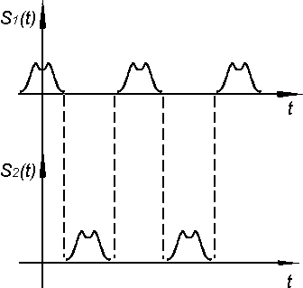
3. Корреляционные характеристики детерминированных сигналов.

Автокорреляционная
характеристика (АКФ) позволяет судить
о степени связи между самим сигналом и
сдвинутой во времени его копией.

Если
сигнал

вещественный, определен на интервале

и имеет ограниченную энергию, то
корреляционная функция вычисляется по
энергии

—
корреляционная функция

Э
– по энергии

временной
сдвиг самого сигнала и его копии.

Для
каждого конкретного значения получается
число.

1.
АКФ – четная функция временного сдвига

При

сходство между сигналом и его копией
наиболее сильно.

,
следовательно, получается максимум.

Этот
максимум равен энергии.

С
увеличением

степень
связи уменьшается. Это уменьшение может
быть немонотонно.

Когда
сигнал обладает большой энергией, но
имеют ограниченную мощность, АКФ
вычисляется по мощности.

функция
четная.

При

максимум равен P.

2.
Для периодического сигнала АКФ периодична
с тем же периодом.

—
временной сдвиг.

АКФ
самого сигнала периодична с тем же
периодом.

3.
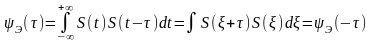
Взаимная корреляционная функция (ВКФ)
позволяет определить степень подобия
двух подобных сигналов.

Пример
(степень
впечатления)

—
ВКФ (не является четной)

Она
позволяет сменить степень сдвига

—
ВКФ нечетная.

Если
у ВКФ есть максимум, то он необязательно
будет при нуле.

При

(нулевом сдвиге)

ВКФ
в этом случае равна взаимной энергии.

АКФ
является частным случаем ВКФ.

Когда
мы хотим наилучшим образом принимать
сигналы (информацию), речь идет об
оптимальном приемнике (он вычисляет
ВКФ между принятым сигналом и тем,
который мы ожидаем, максимум – превышение
над шумами).

4. Разложение сигналов в ряды Фурье. Спектр периодического сигнала.

Задача:
Представить сигнал

,
обладающий конечной мощностью, в виде
суммы (n+1)
некоторых сигналов (задача аппроксимации
— метод, состоящий в замене одних
математических объектов другими, в том
или ином смысле близкими к исходным, но
более простыми. Аппроксимация позволяет
исследовать числовые характеристики
и качественные свойства объекта, сводя
задачу к изучению более простых или
более удобных объектов)

будем считать их попарно ортогональными
на интервале

—
средняя мощность

Произвольный
сигнал конечной мощности

,
заданный на интервале

можно аппроксимировать линейной
комбинацией этих (n+1)
функций.

(2)

—
система попарно ортогональных эталонных
функций – базисная система (базис).

Если
в условии (1)

,
то говорят, что функция

называется нормированной, а

— ортонормированной базисной системой.

Коэффициент

— определяет вес каждого базисного
сигнала. Точность аппроксимации условимся
определять по квадрату разности сигнала
и копии, т.е. ошибка будет:

Коэффициент

определяется из минимума средней
мощности ошибки.

—
среднеквадратичная ошибка.

Учитывая,
что все P>0,

>0,
то можно заметить, что

(2)

– неравенство
Бесселя.

Мощность
копии всегда мощнее мощности оригинала.

Чем
больше n,
тем ближе сумма (2) будет приближаться
к оригиналу, т.е., чем больше слагаемых,
тем меньше среднеквадратическая ошибка.
Этот факт является признаком полного
базиса.

Если
число слагаемых стремиться к бесконечности,
то среднеквадратическая ошибка стремиться
к нулю, т.е.

—
равенство Парсеваля.

В
случае, когда мы хотим получить

—
это ряд сходится к оригиналу.

В
такой ряд можно разложить сигналы
конечной мощности, если базисные функции
попарно ортогональны. Коэффициент

является функцией двух переменных

,
где t
– непрерывная переменная, k
– дискретная переменная.

—
спектр сигнала.

—
спектральная составляющая сигнала.

Сигнал
представлен в виде суммы спектральных
составляющих.

Два
вида представления сигнала:

спектральная
форма
временная

Обе
они однозначно задают сигнал.

Совокупность
коэффициентов ряда часто изображают в
виде отрезка.

Коэффициенты
должны уменьшаться, в общем, с расчетом
номера k.

Т.е.
в пределе

.

Соседние файлы в предмете [НЕСОРТИРОВАННОЕ]

Источник

Макеты страниц

Предположим, что в качестве предсказывающе сглаживающего фильтра на рис. 1 применен фильтр с частотной характеристикой Какова среднеквадратичная ошибка предсказания? Так как различные частоты некогерентны, можно вычислить среднюю мощность ошибки

суммированием составляющих различных частот. Рассмотрим компоненты сигнала и шума на определенной частоте Предполагается, что сигнал и шум некогерентны при всех частотах. Тогда на частоте составляющая ошибки, обусловленная шумом, равна где — средняя мощность шума на частоте

Существует также составляющая ошибки благодаря ослаблению компонент сигнала после прохождения его через фильтр. Для составляющей частоты амплитуды на входе и на выходе должны быть равны, а фаза на выходе должна иметь опережение на Тогда ошибка в мощности будет

где — мощность сигнала на частоте

Общая среднеквадратичная ошибка на частоте является суммой этих двух ошибок, или

и общая среднеквадратичная ошибка для всех частот равна

Задача заключается в минимизации Е надлежащим выбором с учетом того, что система с частотной характеристикой должна быть физически осуществима.

Некоторые важные выводы можно сделать сразу же из рассмотрения выражения (12). Сигнал и шум входят в уравнение только

через посредство их спектров мощности. Следовательно, единственные статистические параметры сигнала и шума, необходимые для решения проблемы, это их спектры. Два различных сигнала с одним и тем же спектром мощности ведут к одному и тому же оптимальному предсказывающему фильтру и к той же самой среднеквадратичной ошибке. Например, если в качестве сигнала используется речь, она может быть предсказана тем же фильтром, который используется для предсказания белого теплового шума, предварительно пропущенного через фильтр, дающий на выходе такой же спектр, как спектр речи.

Говоря более вольно, линейный фильтр может использовать статистику, относящуюся только к амплитудам различных частотных составляющих, статистика фазовых углов этих составляющих не может быть использована. Только нелинейное предсказание может использовать этот статистический эффект для улучшения предсказания.

Ясно, что в проблеме линейной аппроксимации по методу наименьших квадратов можно при желании заменить сигнал и шум любыми временными последовательностями, которые имеют те же спектры мощности. Это никоим образом не изменит оптимального фильтра и среднеквадратичной ошибки.

Источник

УДК 004 421 К. А. КОРОЛЁВА ^

С. С. ГРИЦУТЕНКО ‘

Омский государственный университет путей сообщения

ОПТИМАЛЬНАЯ ИНТЕРПОЛЯЦИЯ УЗКОПОЛОСНОГО СИГНАЛА В СМЫСЛЕ МИНИМУМА СРЕДНЕКВАДРАТИЧНОЙ ОШИБКИ

В статье рассмотрена оптимальная интерполяция сигнала, полоса которого значительно уже половины частоты дискретизации. Критерием оптимальности является минимум среднеквадратичного отклонения интерполированного сигнала от идеального. Оптимизация ведется для различных соотношений полосы сигнала и частоты дискретизации. Приведены результаты моделирования для интерполирующих фильтров разных поряд ко в и по лос пропускания фильтров. Ключевые слова: интерполяция, узкополосный сигнал, фильтр, среднеквадратичная погрешность.

Важнейшей проблемой информатизации железнодорожного транспорта в настоящее время является автоматизация сбора первичной информации и сокращение времени, требуемого на ее обработку. Для решения задач по совершенствованию систем информатизации и связи на железнодорожном транспорте, предоставления новых видов услуг по передаче речи, увеличению общего числа пользователей во всех подразделениях железнодорожного транспорта Министерством путей сообщения РФ было принято решение о создании систем цифровой технологической радиосвязи. Также одной из особенностей современного железнодорожного сообщения является увеличение скорости движения, что влечет за собой возникновение эффекта Доплера, который выражается как в смещении центральной частоты сигнала, так и в деформации его спектра. Восстановление деформированного спектра в данном случае равносильно интерполяции сигнала. В статье рассматривается оптимальная интерполяция сигнала, полоса которого значительно уже половины частоты дискретизации. Критерием оптимальности является минимум среднеквадратичного отклонения интерполированного сигнала от идеального. Оптимизация ведется для различных соотношений полосы сигнала и частоты дискретизации [1—3].

Рассмотрим следующие начальные условия. Пусть s(t) — сигнал, дискретизируемый равномерно с частотой ал. При этом ширина полосы данного

сигнала Aa><<a>d. Результатом дискретизации явля-

2о

ется последовательность s(—Т), где Т = — . Далее

для упрощентя В21кладок будем считать, что T = 1, тогда md = 271, г, следователыго, Дю<<2тс.

Задача состоет в получении такой последовательности ~(иГ + Дг), где At е [0, 1], из последовательности s(nT), чообы выражение

P4(C(nT + Де) — s(nT + Д)))Г г

= рр(н (n + Де) — s(n + Д,))2

(1)

имело минималеное зн(чение при фиксированном N.

Начнем n и+вестной интерпол!ционной формулы Котельникова [4]

нт)г 44- нс)

sin o(t — С) оД — С) ‘

(2)

Таким обраном , если нн+ интересует знгчение сигнала s(t) в некоторой тс)ке t=о+№, то величину s(n+At) можно вычипоить при помощи операции скалярного прорзнедения пр фср>м^е

. n ■Сп ^ sino^^^ — С)

s(n +Д) = 4)н(С)—г

ДтТ o(n + Де — о

= 44 s(-) • Дс

(3)

В (3) количество отсаечов :з(кСи коэффициентов Ьк бесконечно, что делиет невоимпжным реализацию этого алгоритмч в реальнон устройств). Поэтому ограничим их число до N4-1. Однако вотникает вопрос, какие именно из оасчетов з(к) следует использовать для интерполяцик, тлк кас вклад отсчета в точность иктерполяции завоокт от епо расстояния до точки, в котомой скснас онтеупорируют.

Действидеоно, есси интерполяция производится в точке 1=п+Д^ мо

sino(n + Де — С) о (n+Де -С)

sinoДt

тг(п + Де — С)

(4)

откуда однозначно вытекает, что максимальный вклад дают те отсчеты, номера к которых максимально блиоки к лЧ№. Для слрчая четного количества коэффициентов N +1 это означает, что слева

о=0

и справа от точки интерполяции должно находиться ™ N +1

отсчетов, и формула (3) получает вид

,о{п + АО) = п + к — Iх

с1пч АО + к

N +1

ч АО + к —

N +1

+ ^(п + АО) =

N ( N + 1л = ^0 п + О—|Ао + +(п + АО),

к=0 V 2

Фурье, если сигналу к(о) соответствует спектр Я(т), то смещенному на Дt сигналу в/л+Д^ соответствует спектр 8(а)е~->н’.

Тогда рассматриваемая задача оптимизации сводится к нахождению N+1 коэффициентов КИХ фильтра Ьк (соглапно формуле (3) или (4)) с частотной характеристикой, максимально приближенной к форме е-0(I! полосе частот [т , т2], где т1 и т2 — начальная и конегная частоты в спектре интерполируемого сигнала.

Запишем =азложелие фуакции е-■Д] в ряд

(5)

= ЛгеЛ,еЦ°еЛ,еОще… е Ко3′

(8)

где ц(n+Дt) — ошибка, вносимая усечением ряда.

Для случая нечетного количества коэффициентов это ознлч=ет, что точка =нтерполя°ии должна

находиться ближе всего к центральному отсчету

N +1

с номером -, или, что то же самое, на расстоя-

Г 1 Г N .

нии не более чем _ от отсчета о| —е 1

о(п е ЛА) = фЗо[ п е ко Н о 11 о

■ [ л , N 11 с1пн| ЛО е к—-I

о-т^-——j-га е л(п е ЛгО ) =

Н ЛОек

Г Г

фо[ п е к о 0Л о 1 Л -г л(п е ЛО)

Правая часть вN1 раженио (8) представляет собой интерполщующиф многочлен жда

(6)

PN(x) = Л0 +Л1х + Лгхг +… + ЛNxN,

(9)

где х = еН

Таким об разом, задапа св воитое к; по иску массива коэффицикнтов Ь1, Ь2…ЬМ при помощи метода наименьшм квадрагов, чтобы обеспечить выполнение условия (7).

еп нахвждгния коэффициентоы основывается на поисре минимфга Фхнкцли

^ = фф Р (нЛ0K)оH300 =

п=1

н 0 е

= ф )фЗЪи

(10)

Необходимо учитывать, что, согласно начальному условию Дт<<а>л, спекир сигнала s(n+Дt) занимает сравнительно уекую по цлоошению к частоте дискретизации полосу. О зависимости от набора коэффициентов {Ьк} в этуполосу попадаетбольше или меньше; он ер лии оши бко ентее тъоняе,ии ц(п+ДЦ. Выполним оптимизацию данных коэффициентов для минимизхц=л шпи=ли лнторюоляции в полосе сигнала s(t).

Рассмотр=з критерий оптимизации. Пусть интерполированный сигнал подается на решающее устройство, I! оынову работы которого положен критерий м=кcиФaлнноиo п°а вдоы одобия. Ото о зна-чает, что данное =устройптво аравоивает все входящие сигналы с неким набором оталонов. Сравнение заключается в лэхофплнци сроохоквадратичного отклонения входного сигнала от эгалонов. Тот эталон, который имеет наименьшее среднеквадоатич-ное отклонение от сигнала но входх решающего устройства, считается пе^данным сигналом. Следовательно, ми н имиз ациг ошибои и нтерполяции для описанного случая доажна закжочаться в том, чтобы сред=екоa1npaтдондт отклонение интерполированного сигнала ~(п е ЛО) от идеального сигнала s(n+Дt) быио минимальным:

где t — мозент превмен0О двя которого выполняется интерполяция; {тп} — набор точек на оси частот, лежащих на ынтервале [т1, т2].

]Xцве=тнo, что функ+ия ымеег минимумы в точках, в кхто]иы+ 1се час+ные производные равны

СГ

ну=н :

со.

■ = 0, Л = 0, 1…32.

Напишем это в виде системы уравнений с —четом (1иО:

СГ СЪ0

сг.

Сф

сг со,

ГI

П=1

г1

n=]

гТ

Н + оз + ь?» 2 +.

iНе можете найти то, что вам нужно? Попробуйте сервис подбора литературы.

+ Ко’

еы2п и о32

Н + ЪЗ +Лг оПшп +.

+ К,е

НЫ2п и Н32

(11)

Ч + Ь^нг»п +Ъг оПшп + .

+ Ко

3О2п и Н32’г!

В конечном виде выражение для нахождения коэффициентов имеет вид

ф(о(п а ЛО) оИИ(п еЛО ))г

(7)

Среднеквадратичное отклонение двух сигналов возможно вьшислять еок во вхыменной области, так и в частотной, поэтому рассмотрим спектр сигнала s(n+At= Соглнсео CI30]йcтвам преобразования

Ог,Ли + ОТ?322 + Нз132 +… 2 Ъы 1Нт’п = I3

Г!=1

n=] n=]

тГ2n _ , = 3(ы+1).

ЪоТ?32’п нНЦН3^ +… + ЪыI

Н ‘ » = I? » о

n=]

Ъо Т?^ + ъТоН3^2 + + .. + Ъы То32 О2о в I

в > Н3Ыапо3ап’ .

пв! V и=

n=]

пво

n=]

Решение данной системы существует, и оно единственно. Рассчитанный таким способом фильтр с коэффициентами Ьк наилучшим образом интерполирует исходную функцию в среднеквадратичном смысле.

Так как мы оперируем с узкополосными сигналами, то можно оптимизировать распределение величины ошибки не для всей полосы частот, а только для некоторого частотного интервала [5]. А именно, при организации связи на железнодорожном транспорте используются радиостанции, работающие на фиксированных частотах. Кроме того, для каждого вида связи между абонентами предусмотрен свой диапазон частот. Поэтому при передаче сообщений известен используемый диапазон частот. Покажем, что количество вычислений, которые необходимо выполнить при интерполяции, не зависят от центральной частоты этого интервала.

Действительно, если допустить, что при смещении центральной частоты частотного интервала количество необходимых для интерполяции арифметических операций меняется, то воумоуно при помощи элементарных действий сместить спяктр интерполируемого сигнала в ту о бласть, где требуется минимум таких операций, и поуло интеоуоляции вернуть спектр уже интерполированного сигкала обратно. Поэтому дальше будем рассманривать интерполяцию только в частотном интервале [—а; а],

где а

верхняя частота полосы пропускания

интерполирующего фильтра, то есть счятать, что центральная частота ч астятного и бтерв уян находится в нуле.

Проведем моделирование предлагаемого алгоритма. Сформируем трутовый тигнал, стстоящий из К-отсчетов. Спектр сигнала перенесем в область нижних частот так, чтобы его центральная частота находилась в чуле. После пе=лннса сигнала на нулевую частоту проиаведкм ено интерполяцию согласно описанному алгоритму. Лндраоумовается, что в результате интерполяции мы получим набор значений этого сигнаьа между еко отсчттаки. Другими словами, получим ядлинутый сигнал относительно исходного. Про этом величина сдвига интерполированного сигнала относинельно исходного зависит и от порядка интнрполурующего фильтра. Для интерполирующего фильтра порядка N величина сдвига равна

Рис. 1. Распределение среднеквадратичной ошибки интерполяции для фильтров разных порядков от 1 до 10 в зависимости от величины временного сдвига 1

0 0.05 0.1 0.15 0.2 0.25 0.3 0.35 0.4 0.45 0.! т птс с]ота1п

Рис. 2. Среднеквадратичная ошибка интерполяции для полосы пропускания фильтра, равной 10 % от частоты дискретизации, где порядок фильтра для каждой кривой составляет: а — 1; Ь — 2; с — 3; а — 4; е — 5; Г — 6; д — 7; И — 8; 1 — 9; j — 10

ч = М о

а-с л ‘

(13)

где Д е [В, С].

Вычислив значения сргнала, в нужные моменты времени при необходимости сигнал возвращают на несущую частоту. Полученные результаты моделирования демонстрируят распределение погрешности интерполяции в зависимости от заданных пара-метровалгоритма интерполяции.

На рис. 1 представлены кривые распределения среднеквадратичной ошибки интерполяции для фильтров разных кпорядков при полосе пропускания фильтра, равной 10 % от частоты дискретизации, в зависимости от величины сдвига I. Верхняя кривая соответствует фильтру первого порядка, следующие кривые соответствуют фильтрам второго — девятого порядков, нижняя — фильтру десятого порядка. При этом наглядно продемонстрировано, как величина среднеквадратичной ошибки интерполяции зависит от количества коэффици-

ентов N. Так, например, величина среднеквадратичной ошибки для фильтра первого порядка при t = 0,5 составляет порядка —50 дБ, а для фильтра пятого порядка при t = 2,5 — около —95 дБ.

Чем больше порядок фильтра и, соответственно, количество коэффициентов, тем большее число отсчетов сигнала используется и улучшается качество интерполяции в целом. Однако вместе с тем увеличивается и количество операций, требуемых для вычисления значения в произвольной точке.

Так как целью данного исследования является предложение универсального быстродействующего алгоритма для наилучшего приближения исходной функции, рассматриваются фильтры с длиной импульсной характеристики не более десяти.

Верхняя кривая на графике показывает симметричное относительно середины расстояния между известными отсчетами распределение среднеквадратичной ошибки интерполяции для фильтра первого порядка (с длиной импульсной характеристики, равной двум). При этом своего локального максимума она достигает при Дt = 0,5.

Все кривые распределения среднеквадратичной ошибки для фильтров порядка N имеют подобную особенность, а именно симметр ичны относительно

* = N.

Кривые, характеризующие распределение среднеквадратичной ошибки для фильтров нечетного порядка N имеют особенность. Они симметрич-

ны относительно точки —, находящейся посередине между известными отсчетами. Однако следует учитывать, что распределение среднеквадратичной ошибки на интервалах [0; 0,5] и [0,5; 1] не идентично. Поэтому, анализируя полученные зависимости, предложено при интерполяции использовать величину сдвига Дí в интервале [ — 0,5; 0,5]. Это позволяет обеспечить минимально возможное среднеквадратичное отклонение интерполированного сигнала от эталонного.

Зависимости среднеквадратичной ошибки интерполяции сигнала с шириной спектра, составляющей 10 % от частоты дискретизации для фильтров разных порядков, показаны на рис. 2.

Теперь рассмотрим влияние выбора ширины полосы пропускания фильтра на величину ошибки интерполяции. Изображенные на рис. 3 кривые показывают соответственно распределение среднеквадратичной ошибки интерполяции для фильтра третьего порядка в зависимости от ширины полосы пропускания фильтра.

Рассмотрим фильтр с полосой пропускания, равной г % от частоты дискретизации сигнала. При выборе меньших значений г полоса частот, в которой необходимо обеспечить качественную интерполяцию, будет более узкой. Следовательно, при малом порядке N многочлена (9) можно обеспечить удовлетворительный уровень ошибки. Таким образом, чем уже полоса принятого сигнала, тем меньше значение ошибки интерполяции.

Это заключение подтверждают результаты моделирования, представленные на рис. 3. Так, если полоса сигнала составляет 1 % от частоты дискретизации, то среднеквадратичная ошибка интерполяции составляет —220 дБ. Для случая 20 % от частоты дискретизации среднеквадратичная ошибка составляет —90 дБ.

Таким образом, можно подобрать оптимальное соотношение порядка интерполирующего фильтра, в зависимости от ширины спектра интерполируемого сигнала, для заданной величины погрешности.

В статье рассмотрена интерполяция сигналов с шириной полосы частот значительно уже частоты дискретизации. При этом ошибка интерполяции имеет минимальное среднеквадратичное отклонение интерполированного сигнала от идеального для различных соотношений полосы сигнала и частоты дискретизации. Учитывая применяемое оборудование на предприятиях железнодорожного транспорта и специфику организации работы отрасли, рационально менять не дорогостоящие блоки и комплектующие, а алгоритмы обработки принимаемых сигналов. Так, затраты на адаптацию существующей сети не будут дорогостоящими, но выигрыш в качестве обработки будет значительным. Приведены результаты моделирования среднеквадратичной погрешности интерполяции, выполнен сравнительный анализ полученных зависимостей при различных порядках фильтров и величин сдвига. Показано, что вычислительная сложность пред-

Рис. 3. Среднеквадратичная ошибка интерполяции для фильтра третьего порядка, где полоса пропускания

фильтра составляет от частоты дискретизации: a — 45 %; Ь — 20 %; c — 10 %; d — 5 %; e — 2 %; f — 1 %

лагаемого алгоритма, в случае если длина импульсной характеристики фильтров не превышает 10, не отличается от уже применяемых алгоритмов обработки сигналов; однако при восстановлении принятого сообщения точность достигает 90 дБ в относительно широком диапазоне (20 % от частоты дискретизации).

Библиографический список

1. Грицутенко, С. С. Компенсация эффекта Доплера в OFDM-сигнале / С. С. Грицутенко, А. С. Сидоренко // Известия Транссиба. — 2012. — № 3. — С. 100-105.

2. Грицутенко, С. С. Адекватность использования аналогий в цифровой обработке сигналов / С. С. Грицутенко // Известия Транссиба. — 2010. — № 2 (2). — С. 80-86.

3. Галкин, В. А. Цифровая мобильная радиосвязь / В. А. Галкин. — М. : Горячая линия — Телеком, 2007. — 432 с.

4. Biberdorf, E. A new principle of dynamic range expansion by analog-to-digital converting / E. Biberdorf, S. Gritsutenko, K. Firsanov. — Proceedings of IEEE East-West Design & Test Symposium (EWDTS’09) / Kharkov National University of Radioelectronics / Moscow. Russia. September 18-21, 2009, pp. 193-195.

5. Ширман, Я. Д. Теория и техника обработки радиолокационной информации на фоне помех / Я. Д. Ширман, В. Н. Манжос. — М. : Радио и связь, 1981. — 416 с.

КОРОЛЁВА Ксения Андреевна, аспирантка кафедры инфокоммуникационных систем и информационной безопасности Омского государственного университета путей сообщения (ОмГУПС); научный сотрудник Омского научно-исследовательского института приборостроения. Адрес для переписки: jokie-ksu@mail.ru ГРИЦУТЕНКО Станислав Семенович, кандидат технических наук, доцент (Россия), доцент кафедры инфокоммуникационных систем и информационной безопасности, руководитель отдела «Нанотех-нологии» ОмГУПС. Адрес для переписки: st256@mail.ru

Источник

Критерий — среднеквадратичная ошибка

Cтраница 1

Критерий среднеквадратичной ошибки широко используется для систем, находящихся под воздействием стационарных случайных процессов, но он учитывает ошибку лишь в установившемся режиме.
[1]

Оптимальной передаточной функцией при использовании критерия среднеквадратичной ошибки ( СКО) является такая передаточная функция системы, при которой средне квадр этическая ошибка имеет минимум.
[2]

Задача идентификации сводится к определению коэффициентов разложения ядер, минимизирующих критерий среднеквадратичной ошибки между выходами объекта и модели. Применение в качестве изучающего сигнала, сигнала, близкого по своим свойствам к нормальному белому щуму, позволяет значительно упростить алгоритм идентификации и повысить его точность.
[3]

Преобразование Карунена — Лоэва является оптимальным преобразованием для представления сигналов по отношению к критерию среднеквадратичной ошибки.
[4]

Винер в качестве критерия использовал минимизацию среднеквадратичной ошибки, причем, Винер указал [4], что возможны другие критерии, но математическая трактовка упрощается при использовании критерия среднеквадратичной ошибки. Минимизация среднеквадратичной ошибки соответствует минимизации мощности сигнала ошибки, и если дальнейшее кодирование не производится, то это — разумный критерий для случая кодирования с предсказанием. Однако в схеме, приведенной на рис. 1, сигнал ошибки до передачи кодируется и его мощность может быть существенно изменена в процессе кодирования. Больше всего мы заинтересованы в минимизации емкости канала, которая потребуется для передачи сигнала ошибки.
[5]

Рассмотрим также характер использовавшихся нами критериев. Как критерий среднеквадратичной ошибки, так и критерия разброса представляют собой математические ожидания некоторых квадратичных функций переменных.
[6]

Ясно, что в смысле второй постановки линейное безынерционное преобразование бесцельно, в то время как улучшение приближения в смысле среднеквадратичной ошибки в этом случае оказывается значительным. Поэтому в задачах, где существенно выделение формы полезного сигнала, критерий среднеквадратичной ошибки может оказаться неприемлемым.
[7]

При передаче информации др. видов более удобными для оценки помехоустойчивости оказываются др. вероятностные критерии, в частности критерий среднеквадратичной ошибки на выходе системы при заданном О. Такой критерий используется при анализе систем автоматич. В ТУ широко пользуются критериями подавления и возникновения ложной команды, н др. случаях — иными критериями оптимальности. При применении этих критериев необходимо определять более сложные статистич. Все эти критерии находятся при определенном О.
[8]

При передаче информации др. видов более удобными для оценки помехоустойчивости оказываются др. вероятностные критерии, в частности критерий среднеквадратичной ошибки на выходе системы при заданном О. Такой критерий используется при анализе систем автоматич. В ТУ широко пользуются критериями подавления и возникновения ложной команды, и др. случаях — иными критериями оптимальности. При применении этих критериев необходимо определять более сложные статистич. Все эти критерии находятся при определенном О.
[9]

Замечания, ( i) В формулах ( 78) и ( 79) предполагается, что вероятность попадания входного значения х на границы многогранников Вороного пренебрежимо мала. И) Множитель 1 / п вводится для того, чтобы честно сравнивать квантизаторы разных размерностей, ( iii) Критерий среднеквадратичной ошибки — это лишь один из многих возможных способов измерить искажение; его преимущества состоят в широкой употребительности и математической простоте. При применениях к обработке речи и изображения правильный выбор меры искажения является трудной задачей.
[10]

Степень искажений принятого сигнала обычно оценивают по верности его воспроизведения. Под верностью часто понимают среднеквадратичную ошибку, отличающую принятый сигнал от переданного. Необходимо подчеркнуть, что критерий среднеквадратичной ошибки является информационно неверным. Принципиально более правильно оценивать искажения сигнала как появление ложной, ошибочной информации, не поддающейся устранению с помощью коррекции. Искажения, поддающиеся коррекции, как было показано, не изменяют количества информации, а потому здесь не рассматриваются.
[11]

В книге коллектива американских авторов под редакцией Джеймса, Ни-колса и Филипса Теория следящих систем, выпущенной в 1947 г., дан метод построения следящих систем на базе заданного показателя колебательности, а также на основе критерия среднеквадратичной ошибки, предложенного в СССР А. А. Харкевичем в 1937 г. и в США Холлом в 1943 г. Основываясь на идеях А. Н. Колмогорова, высказанных в 1941 г. и развитых им в 1949 г., Винер разрабатывает метод наилучшего линейного фильтра, удовлетворяющего критерию наименьшей среднеквадратичной ошибки.
[12]

Данный результат позволяет глубже проникнуть в суть процедуры, обеспечивающей решение по методу наименьшей квадратичной ошибки. Аппроксимируя g0 ( x), разделяющая функция а у дает непосредственную информацию относительно апостериорных вероятностей Р ( со. К сожалению, критерий среднеквадратичной ошибки в основном распространяется не на точки, близкие к поверхности решения go ( x) 0, а на точки, для которых значение р ( х) велико. Таким образом, разделяющая функция, которая наилучшим образом аппроксимирует разделяющую функцию Байеса, не обязательно минимизирует вероятность ошибки. Несмотря на данный недостаток, решение по методу наименьшей квадратичной ошибки обладает интересными свойствами и широко распространено в литературе.
[14]

В данной главе показано, что ортогональные преобразования можно использовать для сжатия данных. Показано, что ПКЛ является оптимальным преобразованием для сжатия данных по отношению к критерию среднеквадратичной ошибки.
[15]

Страницы:

Источник

Среднеквадратичная ошибка (Mean Squared Error) – Среднее арифметическое (Mean) квадратов разностей между предсказанными и реальными значениями Модели (Model) Машинного обучения (ML):

MSE как среднее дистанций между предсказаниями и реальными наблюдениями

Рассчитывается с помощью формулы, которая будет пояснена в примере ниже:

$$MSE = frac{1}{n} × sum_{i=1}^n (y_i — widetilde{y}_i)^2$$
$$MSEspace{}{–}space{Среднеквадратическая}space{ошибка,}$$
$$nspace{}{–}space{количество}space{наблюдений,}$$
$$y_ispace{}{–}space{фактическая}space{координата}space{наблюдения,}$$
$$widetilde{y}_ispace{}{–}space{предсказанная}space{координата}space{наблюдения,}$$

MSE практически никогда не равен нулю, и происходит это из-за элемента случайности в данных или неучитывания Оценочной функцией (Estimator) всех факторов, которые могли бы улучшить предсказательную способность.

Пример. Исследуем линейную регрессию, изображенную на графике выше, и установим величину среднеквадратической Ошибки (Error). Фактические координаты точек-Наблюдений (Observation) выглядят следующим образом:

Мы имеем дело с Линейной регрессией (Linear Regression), потому уравнение, предсказывающее положение записей, можно представить с помощью формулы:

$$y = M * x + b$$
$$yspace{–}space{значение}space{координаты}space{оси}space{y,}$$
$$Mspace{–}space{уклон}space{прямой}$$
$$xspace{–}space{значение}space{координаты}space{оси}space{x,}$$
$$bspace{–}space{смещение}space{прямой}space{относительно}space{начала}space{координат}$$

Параметры M и b уравнения нам, к счастью, известны в данном обучающем примере, и потому уравнение выглядит следующим образом:

$$y = 0,5252 * x + 17,306$$

Зная координаты реальных записей и уравнение линейной регрессии, мы можем восстановить полные координаты предсказанных наблюдений, обозначенных серыми точками на графике выше. Простой подстановкой значения координаты x в уравнение мы рассчитаем значение координаты ỹ:

Рассчитаем квадрат разницы между Y и Ỹ:

Сумма таких квадратов равна 4 445. Осталось только разделить это число на количество наблюдений (9):

$$MSE = frac{1}{9} × 4445 = 493$$

Само по себе число в такой ситуации становится показательным, когда Дата-сайентист (Data Scientist) предпринимает попытки улучшить предсказательную способность модели и сравнивает MSE каждой итерации, выбирая такое уравнение, что сгенерирует наименьшую погрешность в предсказаниях.

MSE и Scikit-learn

Среднеквадратическую ошибку можно вычислить с помощью SkLearn. Для начала импортируем функцию:

import sklearn
from sklearn.metrics import mean_squared_error

Инициализируем крошечные списки, содержащие реальные и предсказанные координаты y:

y_true = [5, 41, 70, 77, 134, 68, 138, 101, 131]
y_pred = [23, 35, 55, 90, 93, 103, 118, 121, 129]

Инициируем функцию mean_squared_error(), которая рассчитает MSE тем же способом, что и формула выше:

mean_squared_error(y_true, y_pred)

Интересно, что конечный результат на 3 отличается от расчетов с помощью Apple Numbers:

496.0

Ноутбук, не требующий дополнительной настройки на момент написания статьи, можно скачать здесь.

Автор оригинальной статьи: @mmoshikoo

Фото: @tobyelliott

Источник