Содержание
- Расчет ошибки средней арифметической
- Способ 1: расчет с помощью комбинации функций
- Способ 2: применение инструмента «Описательная статистика»
- Вопросы и ответы

Стандартная ошибка или, как часто называют, ошибка средней арифметической, является одним из важных статистических показателей. С помощью данного показателя можно определить неоднородность выборки. Он также довольно важен при прогнозировании. Давайте узнаем, какими способами можно рассчитать величину стандартной ошибки с помощью инструментов Microsoft Excel.
Расчет ошибки средней арифметической
Одним из показателей, которые характеризуют цельность и однородность выборки, является стандартная ошибка. Эта величина представляет собой корень квадратный из дисперсии. Сама дисперсия является средним квадратном от средней арифметической. Средняя арифметическая вычисляется делением суммарной величины объектов выборки на их общее количество.
В Экселе существуют два способа вычисления стандартной ошибки: используя набор функций и при помощи инструментов Пакета анализа. Давайте подробно рассмотрим каждый из этих вариантов.
Способ 1: расчет с помощью комбинации функций
Прежде всего, давайте составим алгоритм действий на конкретном примере по расчету ошибки средней арифметической, используя для этих целей комбинацию функций. Для выполнения задачи нам понадобятся операторы СТАНДОТКЛОН.В, КОРЕНЬ и СЧЁТ.
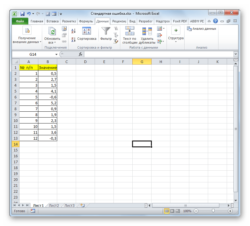
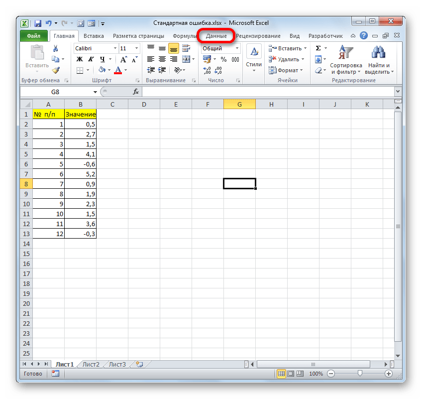
Для примера нами будет использована выборка из двенадцати чисел, представленных в таблице.
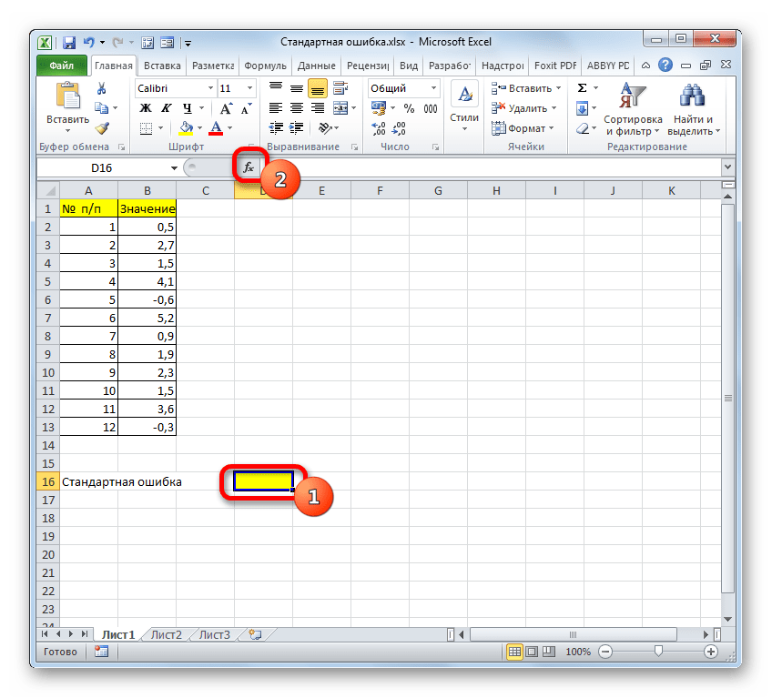
- Выделяем ячейку, в которой будет выводиться итоговое значение стандартной ошибки, и клацаем по иконке «Вставить функцию».
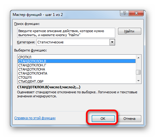
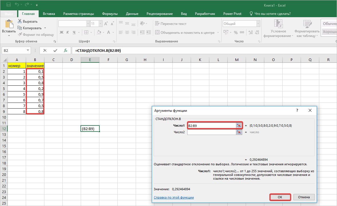
- Открывается Мастер функций. Производим перемещение в блок «Статистические». В представленном перечне наименований выбираем название «СТАНДОТКЛОН.В».
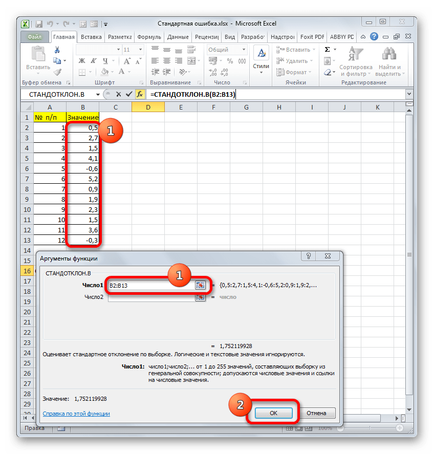
- Запускается окно аргументов вышеуказанного оператора. СТАНДОТКЛОН.В предназначен для оценивания стандартного отклонения при выборке. Данный оператор имеет следующий синтаксис:
=СТАНДОТКЛОН.В(число1;число2;…)«Число1» и последующие аргументы являются числовыми значениями или ссылками на ячейки и диапазоны листа, в которых они расположены. Всего может насчитываться до 255 аргументов этого типа. Обязательным является только первый аргумент.
Итак, устанавливаем курсор в поле «Число1». Далее, обязательно произведя зажим левой кнопки мыши, выделяем курсором весь диапазон выборки на листе. Координаты данного массива тут же отображаются в поле окна. После этого клацаем по кнопке «OK».
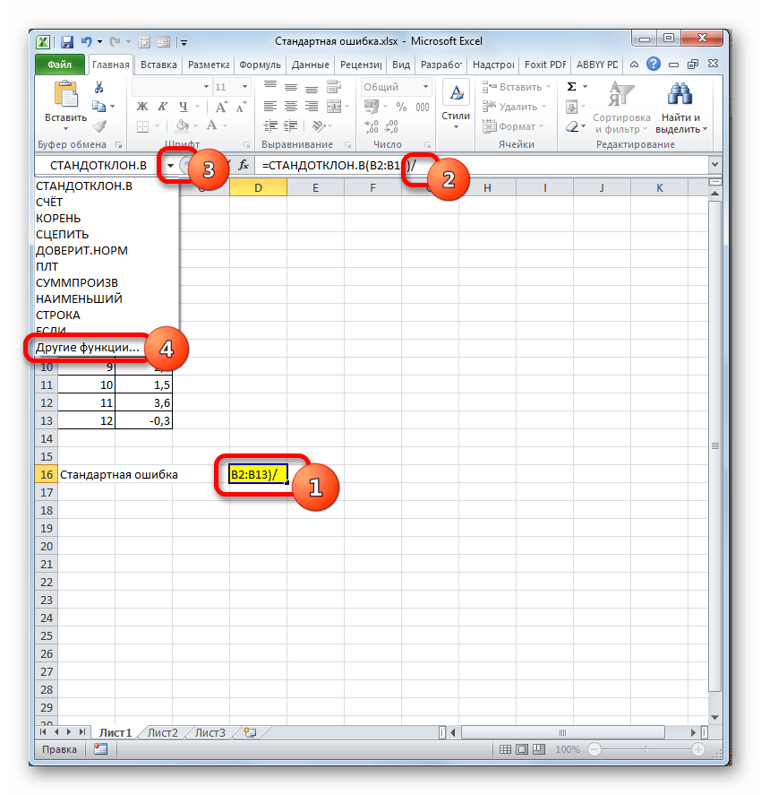
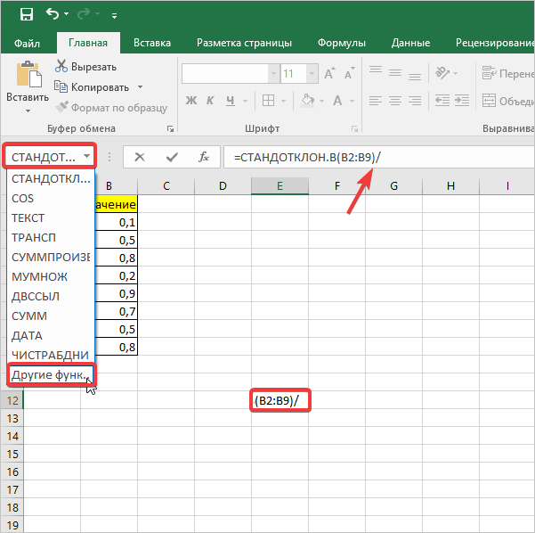
- В ячейку на листе выводится результат расчета оператора СТАНДОТКЛОН.В. Но это ещё не ошибка средней арифметической. Для того, чтобы получить искомое значение, нужно стандартное отклонение разделить на квадратный корень от количества элементов выборки. Для того, чтобы продолжить вычисления, выделяем ячейку, содержащую функцию СТАНДОТКЛОН.В. После этого устанавливаем курсор в строку формул и дописываем после уже существующего выражения знак деления (/). Вслед за этим клацаем по пиктограмме перевернутого вниз углом треугольника, которая располагается слева от строки формул. Открывается список недавно использованных функций. Если вы в нем найдете наименование оператора «КОРЕНЬ», то переходите по данному наименованию. В обратном случае жмите по пункту «Другие функции…».
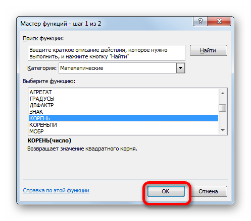
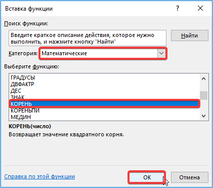
- Снова происходит запуск Мастера функций. На этот раз нам следует посетить категорию «Математические». В представленном перечне выделяем название «КОРЕНЬ» и жмем на кнопку «OK».
- Открывается окно аргументов функции КОРЕНЬ. Единственной задачей данного оператора является вычисление квадратного корня из заданного числа. Его синтаксис предельно простой:
=КОРЕНЬ(число)
Как видим, функция имеет всего один аргумент «Число». Он может быть представлен числовым значением, ссылкой на ячейку, в которой оно содержится или другой функцией, вычисляющей это число. Последний вариант как раз и будет представлен в нашем примере.
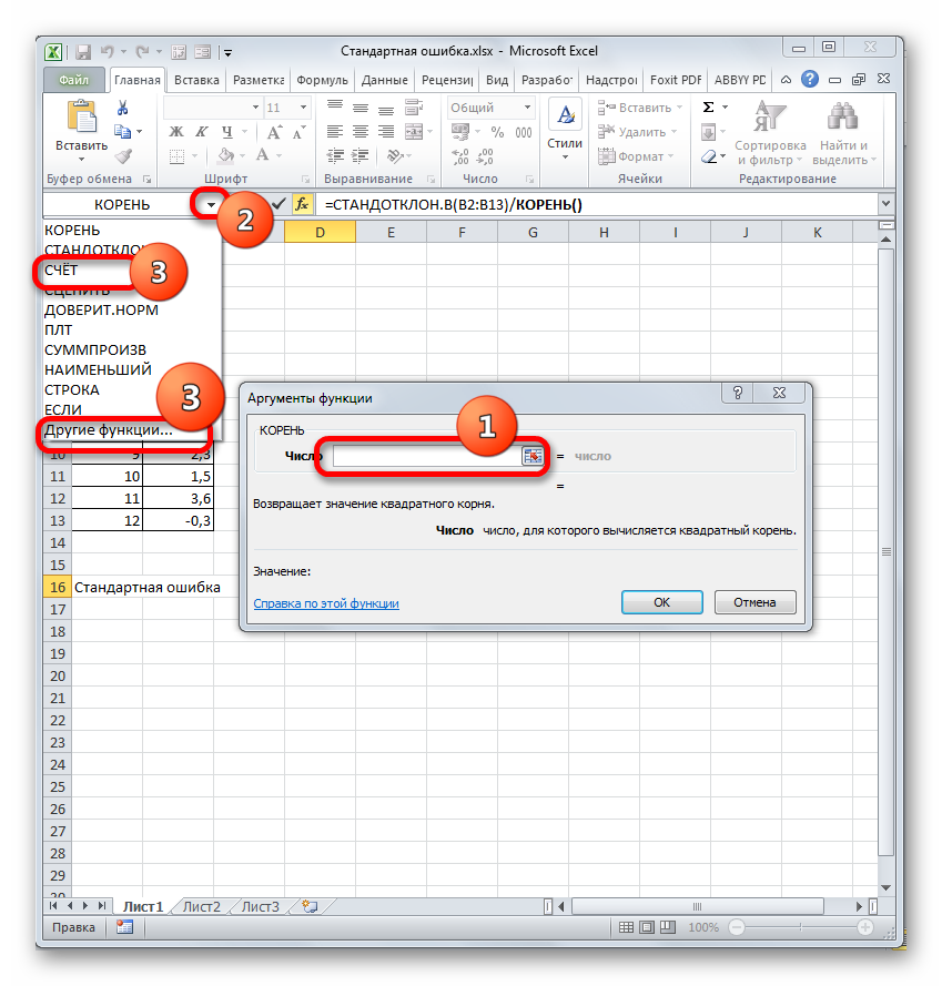
Устанавливаем курсор в поле «Число» и кликаем по знакомому нам треугольнику, который вызывает список последних использованных функций. Ищем в нем наименование «СЧЁТ». Если находим, то кликаем по нему. В обратном случае, опять же, переходим по наименованию «Другие функции…».
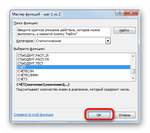
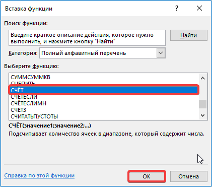
- В раскрывшемся окне Мастера функций производим перемещение в группу «Статистические». Там выделяем наименование «СЧЁТ» и выполняем клик по кнопке «OK».
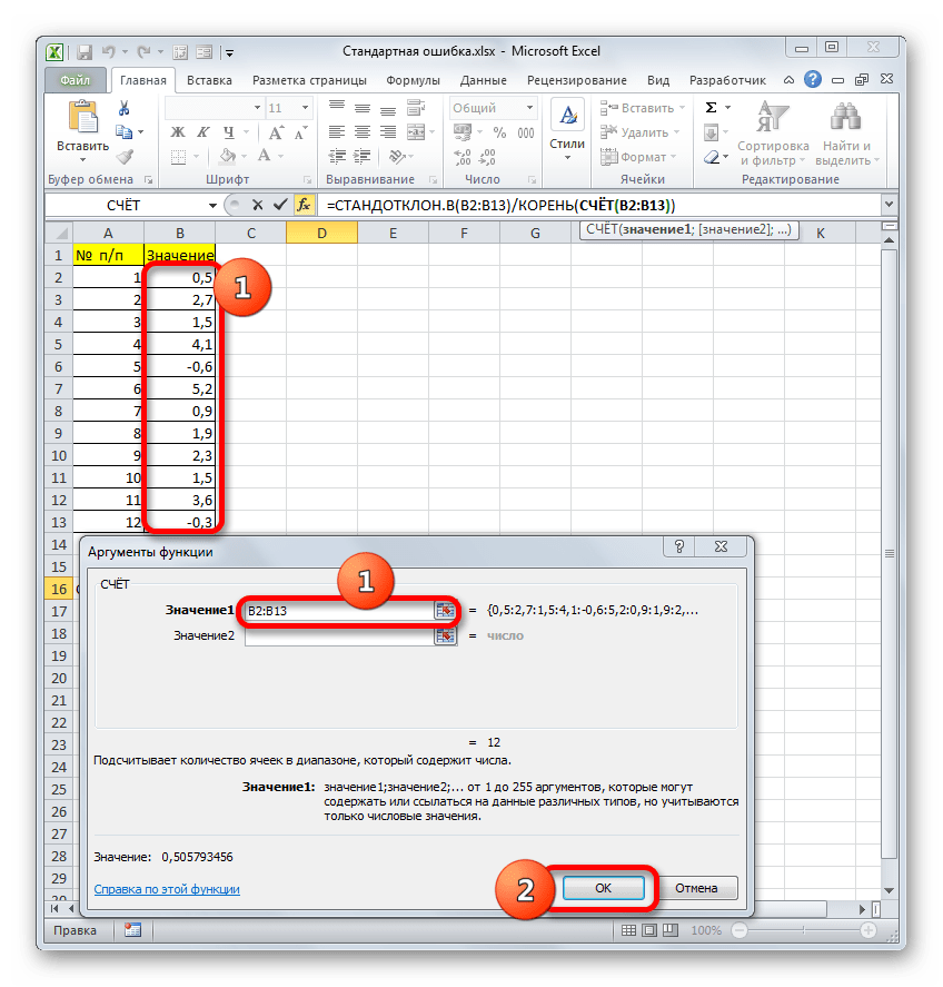
- Запускается окно аргументов функции СЧЁТ. Указанный оператор предназначен для вычисления количества ячеек, которые заполнены числовыми значениями. В нашем случае он будет подсчитывать количество элементов выборки и сообщать результат «материнскому» оператору КОРЕНЬ. Синтаксис функции следующий:
=СЧЁТ(значение1;значение2;…)В качестве аргументов «Значение», которых может насчитываться до 255 штук, выступают ссылки на диапазоны ячеек. Ставим курсор в поле «Значение1», зажимаем левую кнопку мыши и выделяем весь диапазон выборки. После того, как его координаты отобразились в поле, жмем на кнопку «OK».
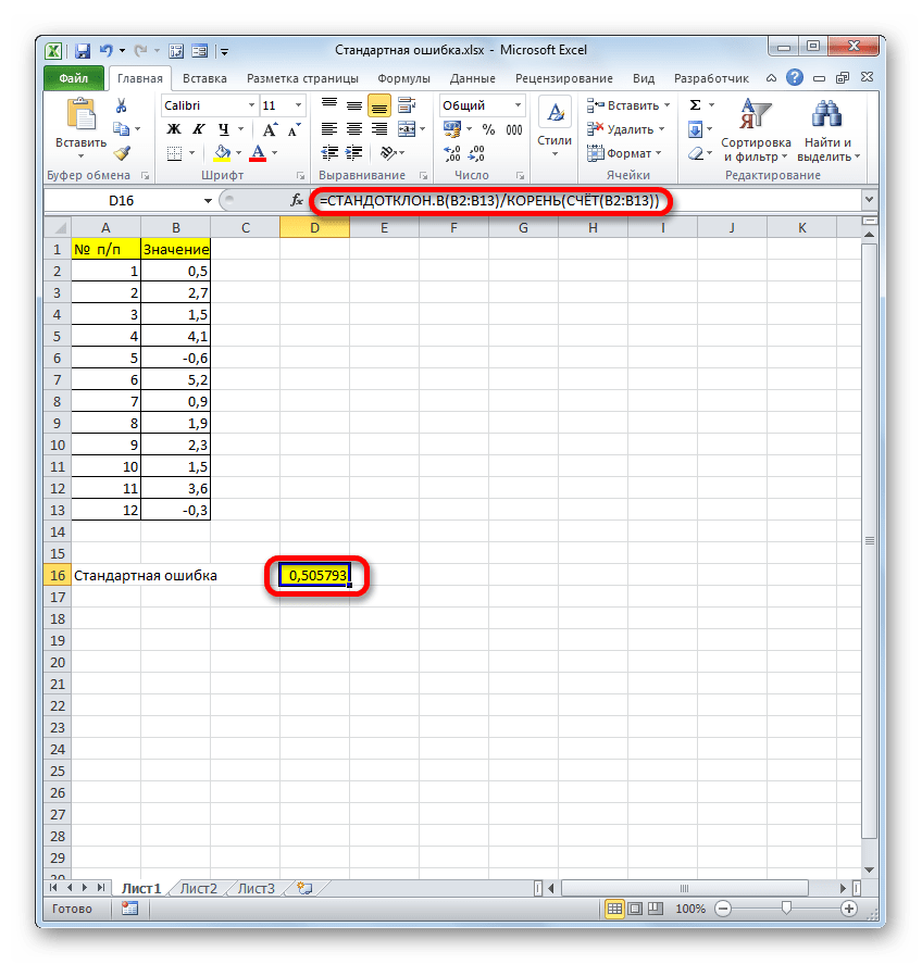
- После выполнения последнего действия будет не только рассчитано количество ячеек заполненных числами, но и вычислена ошибка средней арифметической, так как это был последний штрих в работе над данной формулой. Величина стандартной ошибки выведена в ту ячейку, где размещена сложная формула, общий вид которой в нашем случае следующий:
=СТАНДОТКЛОН.В(B2:B13)/КОРЕНЬ(СЧЁТ(B2:B13))Результат вычисления ошибки средней арифметической составил 0,505793. Запомним это число и сравним с тем, которое получим при решении поставленной задачи следующим способом.

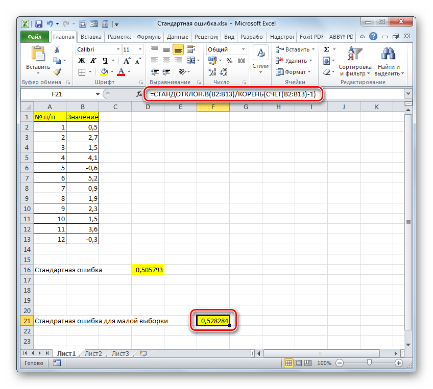
Но дело в том, что для малых выборок (до 30 единиц) для большей точности лучше применять немного измененную формулу. В ней величина стандартного отклонения делится не на квадратный корень от количества элементов выборки, а на квадратный корень от количества элементов выборки минус один. Таким образом, с учетом нюансов малой выборки наша формула приобретет следующий вид:
=СТАНДОТКЛОН.В(B2:B13)/КОРЕНЬ(СЧЁТ(B2:B13)-1)
Урок: Статистические функции в Экселе
Способ 2: применение инструмента «Описательная статистика»
Вторым вариантом, с помощью которого можно вычислить стандартную ошибку в Экселе, является применение инструмента «Описательная статистика», входящего в набор инструментов «Анализ данных» («Пакет анализа»). «Описательная статистика» проводит комплексный анализ выборки по различным критериям. Одним из них как раз и является нахождение ошибки средней арифметической.
Но чтобы воспользоваться данной возможностью, нужно сразу активировать «Пакет анализа», так как по умолчанию в Экселе он отключен.
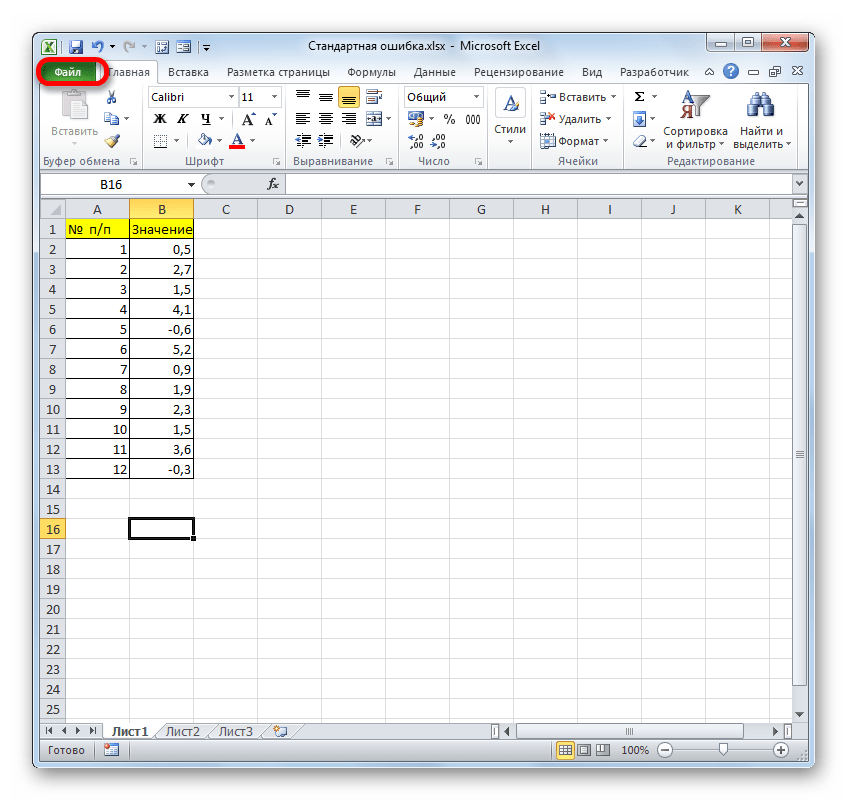
- После того, как открыт документ с выборкой, переходим во вкладку «Файл».
- Далее, воспользовавшись левым вертикальным меню, перемещаемся через его пункт в раздел «Параметры».
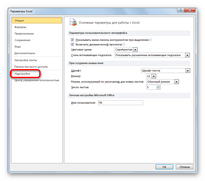
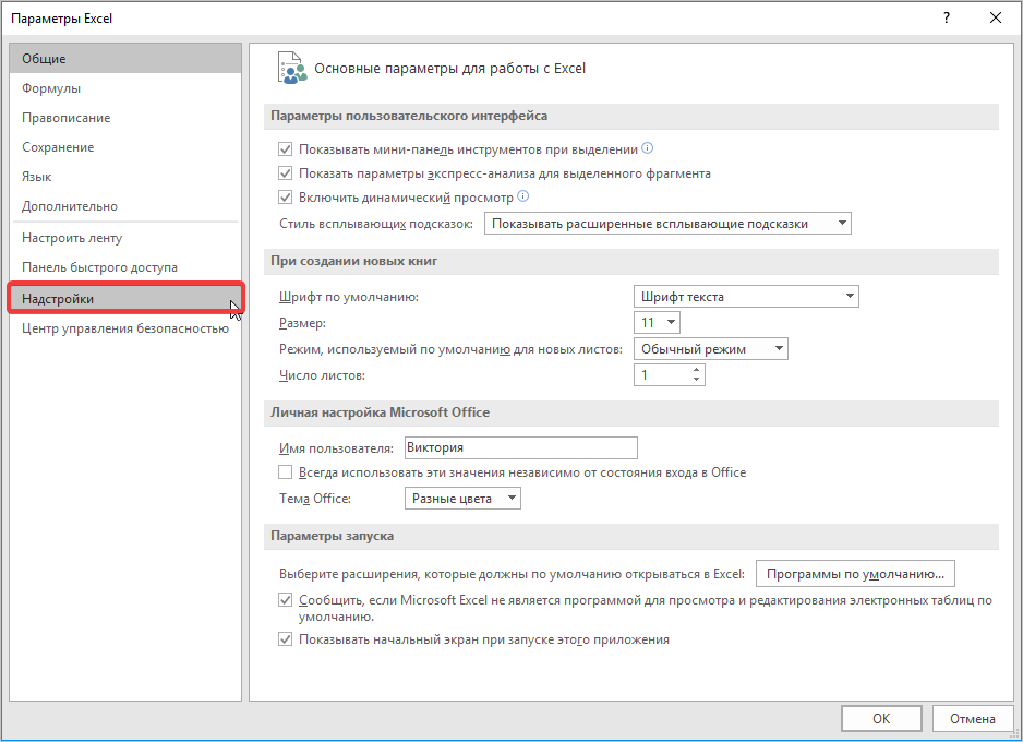
- Запускается окно параметров Эксель. В левой части данного окна размещено меню, через которое перемещаемся в подраздел «Надстройки».
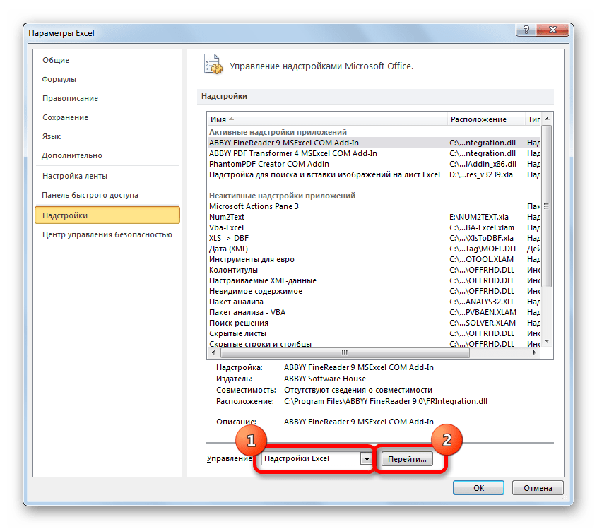
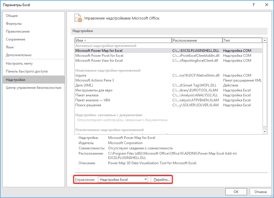
- В самой нижней части появившегося окна расположено поле «Управление». Выставляем в нем параметр «Надстройки Excel» и жмем на кнопку «Перейти…» справа от него.
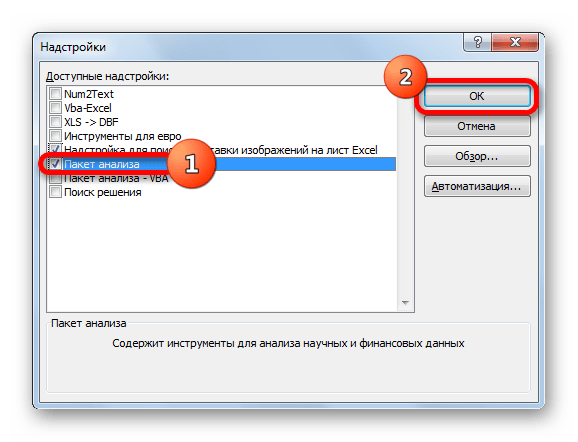
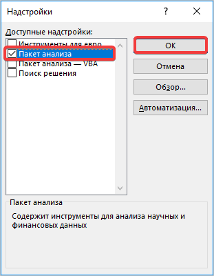
- Запускается окно надстроек с перечнем доступных скриптов. Отмечаем галочкой наименование «Пакет анализа» и щелкаем по кнопке «OK» в правой части окошка.
- После выполнения последнего действия на ленте появится новая группа инструментов, которая имеет наименование «Анализ». Чтобы перейти к ней, щелкаем по названию вкладки «Данные».
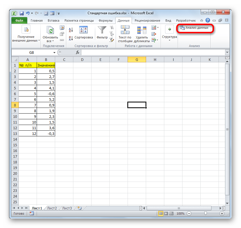
- После перехода жмем на кнопку «Анализ данных» в блоке инструментов «Анализ», который расположен в самом конце ленты.
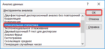
- Запускается окошко выбора инструмента анализа. Выделяем наименование «Описательная статистика» и жмем на кнопку «OK» справа.
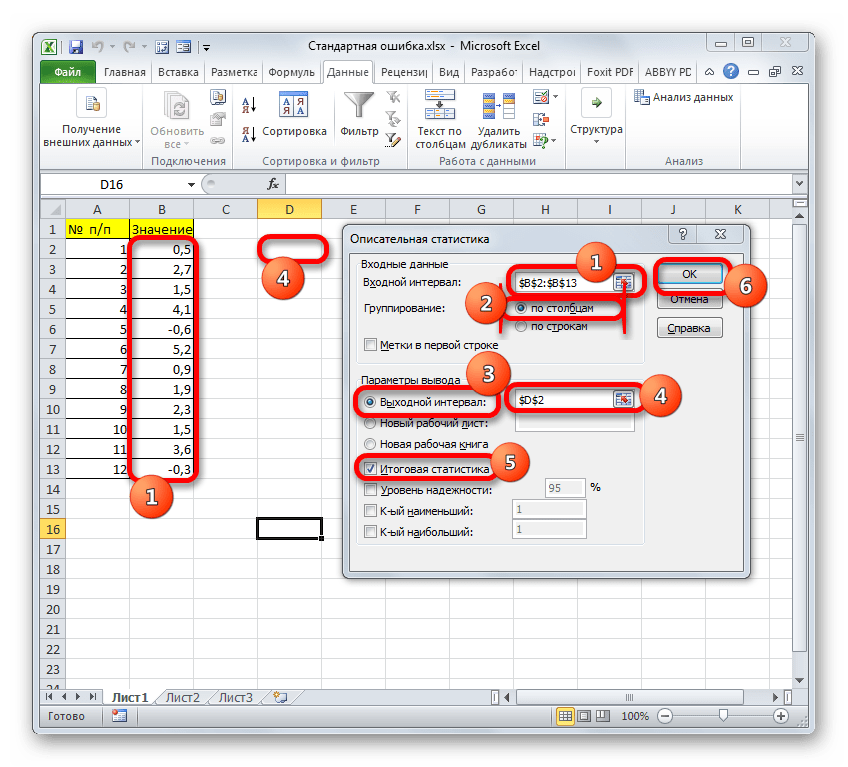
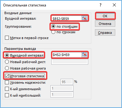
- Запускается окно настроек инструмента комплексного статистического анализа «Описательная статистика».
В поле «Входной интервал» необходимо указать диапазон ячеек таблицы, в которых находится анализируемая выборка. Вручную это делать неудобно, хотя и можно, поэтому ставим курсор в указанное поле и при зажатой левой кнопке мыши выделяем соответствующий массив данных на листе. Его координаты тут же отобразятся в поле окна.
В блоке «Группирование» оставляем настройки по умолчанию. То есть, переключатель должен стоять около пункта «По столбцам». Если это не так, то его следует переставить.
Галочку «Метки в первой строке» можно не устанавливать. Для решения нашего вопроса это не важно.
Далее переходим к блоку настроек «Параметры вывода». Здесь следует указать, куда именно будет выводиться результат расчета инструмента «Описательная статистика»:
- На новый лист;
- В новую книгу (другой файл);
- В указанный диапазон текущего листа.
Давайте выберем последний из этих вариантов. Для этого переставляем переключатель в позицию «Выходной интервал» и устанавливаем курсор в поле напротив данного параметра. После этого клацаем на листе по ячейке, которая станет верхним левым элементом массива вывода данных. Её координаты должны отобразиться в поле, в котором мы до этого устанавливали курсор.
Далее следует блок настроек определяющий, какие именно данные нужно вводить:
- Итоговая статистика;
- К-ый наибольший;
- К-ый наименьший;
- Уровень надежности.
Для определения стандартной ошибки обязательно нужно установить галочку около параметра «Итоговая статистика». Напротив остальных пунктов выставляем галочки на свое усмотрение. На решение нашей основной задачи это никак не повлияет.
После того, как все настройки в окне «Описательная статистика» установлены, щелкаем по кнопке «OK» в его правой части.
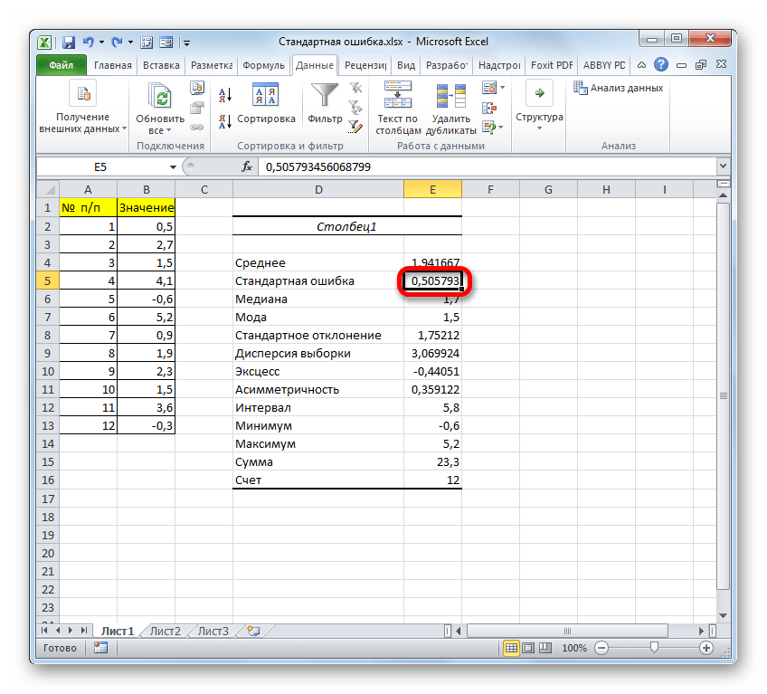
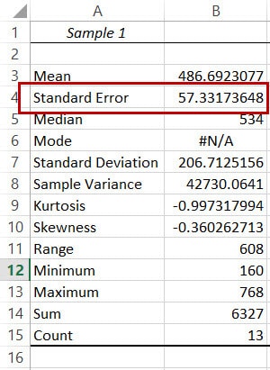
- После этого инструмент «Описательная статистика» выводит результаты обработки выборки на текущий лист. Как видим, это довольно много разноплановых статистических показателей, но среди них есть и нужный нам – «Стандартная ошибка». Он равен числу 0,505793. Это в точности тот же результат, который мы достигли путем применения сложной формулы при описании предыдущего способа.


Урок: Описательная статистика в Экселе
Как видим, в Экселе можно произвести расчет стандартной ошибки двумя способами: применив набор функций и воспользовавшись инструментом пакета анализа «Описательная статистика». Итоговый результат будет абсолютно одинаковый. Поэтому выбор метода зависит от удобства пользователя и поставленной конкретной задачи. Например, если ошибка средней арифметической является только одним из многих статистических показателей выборки, которые нужно рассчитать, то удобнее воспользоваться инструментом «Описательная статистика». Но если вам нужно вычислить исключительно этот показатель, то во избежание нагромождения лишних данных лучше прибегнуть к сложной формуле. В этом случае результат расчета уместится в одной ячейке листа.
Most people use spreadsheets software such as Microsoft Excel to process their data and carry out their analysis tasks.
When performing an analysis of data, a number of statistical metrics come into play. Some of these include the means, the medians, standard deviations, and standard errors. These metrics help in understanding the true nature of the data.
In this article, I will show you two ways to calculate the Standard Error in Excel.
One of the methods involves using a formula and the other involves using a Data Analytics Tool Pack that usually comes with every copy of Excel.
So let’s get started!
What is Standard Error?
When working with real-world data, it is often not possible to work with data of the entire population. So we usually take random samples from the population and work with them.
The standard error of a sample tells how accurate its mean is in terms of the true population mean.
In other words, the standard error of a sample is its standard deviation from the population mean.
This helps analyze how accurately your sample’s mean represents the true population. It also helps analyze the amount of dispersion or variation between your different data samples.
How is Standard Error Calculated?
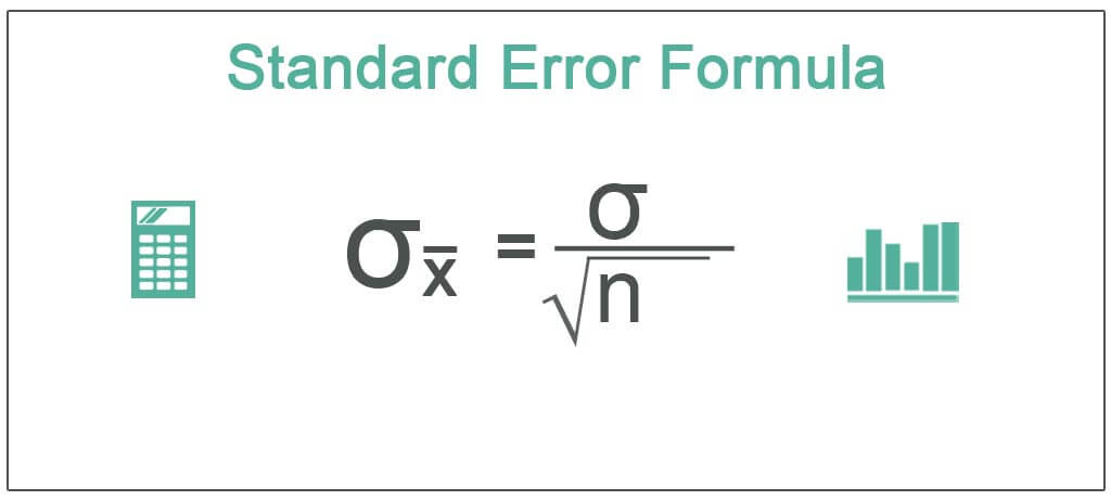
The Standard Error for a sample is usually calculated using the formula:
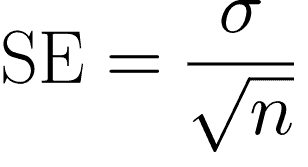
In this above formula:
- SE is Standard Error
- σ represents the Standard deviation of the sample
- n represents the sample size.
How to Find the Standard Error in Excel Using a Formula
Unfortunately, unlike the Standard Deviation, Excel does not have a built-in formula to calculate the Standard Error, at least not at the time of writing this tutorial.
However, you could use the above formula to easily and quickly calculate the standard error. Here are the steps you need to follow:
- Click on the cell where you want the Standard Error to appear and click on the formula bar next to the fx symbol just below your toolbar.
- Type the symbol ‘=’ in the formula bar. And type: =STDEV(
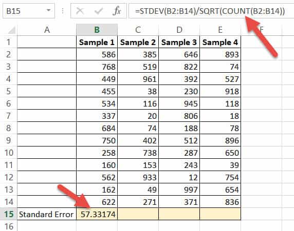
- Drag and select the range of cells that are part of your sample data. This will add the location of the range in your formula. So, if your sample data is in cells B2 to B14, you will see: =STDEV(B2:B14 in the formula bar.
- Close the bracket for the STDEV formula. So far, you have used the STDEV function to find the Standard deviation of your sample data.
- Next, we want to divide this Standard deviation by the square root of the sample size. So let’s continue with our formula. Click on the formula bar after the closing brackets of the STDEV formula and add a ‘/’ symbol to indicate that you want to divide the result of the STDEV function. So your formula so far is: =STDEV(B2:B14)/
- To find the square root of a number, we use the SQRT formula. So next, type SQRT(. Your formula bar will now have the formula: =STDEV(B2:B14)/SQRT(
- Finally, you want the sample size. For this, you need to use the COUNT function. So, type COUNT( after what you already have in your formula bar. Again, drag and select the range of cells that are part of your sample data and close the bracket for the COUNT formula. This will give you the number of cells in your selected range.
- Close the bracket for the SQRT function too. So your final formula should look like this: =STDEV(B2:B14)/SQRT(COUNT(B2:B14)) Notice there are two closing braces in the end. One is for the COUNT function, the other is for the SQRT function.
- That’s it! Press the return key on your keyboard and you got your sample’s Standard Error!
To find the Standard errors for the other samples, you can apply the same formula to these samples too.
If your samples are placed in columns adjacent to one another (as shown in the above image), you only need to drag the fill handle (located at the bottom left corner of your calculated cell) to the right.
This will copy the same formula to all the other cells on the right, and you will get standard errors for each of your samples!
How to Find the Standard Error in Excel Using the Data Analysis Toolpak
If you’re not in the mood to type complex formulae, there’s an easier way to find not just the Standard error, but practically all the statistical metrics you might need to analyze your sample data.
For this, you will need to install the Data Analysis Toolpak. This package gives you access to a variety of statistical functions, which include correlation functions, z-test, and t-test functions too.
Once you install the package, you can use the tool whenever you need to analyze data, without having to re-install it each time.
The Data Analysis Toolpak is free to use and comes along with your Excel package, but for simplicity, it does not appear in your standard toolbar. You need to activate it in order for it to be added to your toolbar.
The process of activating it is quite simple. Just follow these steps to install and activate your Data Analysis Toolpak:
- Click the File tab and click on Options. This will open the Options window for you.
- From here, click “Add-ins” from the left sidebar.
- From the list of Add-ins, select Analysis ToolPak.
- At the bottom of the window, click on the ‘Go’ button just next to Manage: Add-ins.
- Click the checkmark for Analysis ToolPak and click OK.
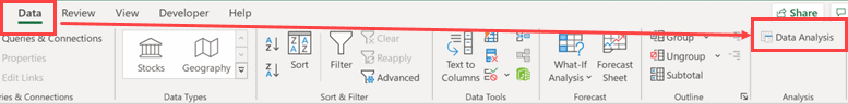
With this, your Data Analysis Toolpak will get added to your Excel Toolbar. When you click the Excel ‘Data’ tab, you should find a tool named “Data Analysis” at the far right of the Data toolbar (under the ‘Analysis’ group).
Now, to find out your Standard Error and other Statistical metrics, do the following:
- Click on the Data Analysis tool under the Data tab. This will open the Analysis Tools dialog box.
- Select “Descriptive Statistics” from the list on the left of the dialog box and click OK.
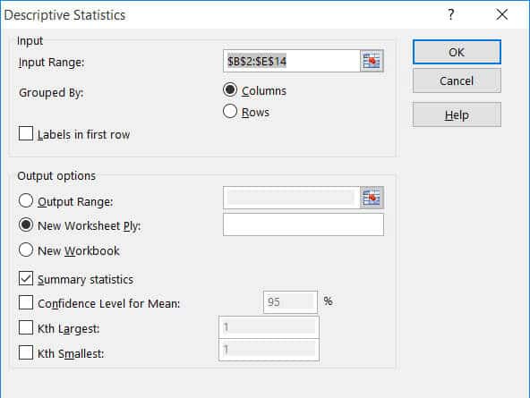
- Enter the location of the range of cells that contain your sample data into the “Input Range” box. You can also choose to drag and select the range of cells that you need too. If you have data for more than one sample arranged in adjacent columns, you can select the data in all the columns. You will get your results separately for each column.
- If your data has column headers, check the “Labels in first row” box.
- Select where you want your results to be displayed. It is safer to select “New Worksheet”. This will ensure that the details get displayed on a newly created worksheet, and will not disturb any data on your current worksheet.
- Select the checkbox next to “Summary Statistics” and click OK.
This will display all your analytical metrics in a new worksheet.
These metrics will also include the Standard Error for your selected sample data. If you had selected multiple data sets in multiple columns, you will get analytics for each column separately.
Conclusion
In this article, we discussed two ways in which you can find the Standard error for your sample data.
You can either create a formula to calculate it or use a data analytics tool, like the Data Analysis Toolpak that comes with Excel.
Either way, you will be able to use the Standard error information to analyze your sample data for further processing.
Hope you found this Excel tutorial useful!
Other Excel tutorials you may find useful:
- How to Convert Decimal to Fraction in Excel
- How to Square a Number in Excel
- How to Subtract Multiple Cells from One Cell in Excel
- How to Find Range in Excel
- How to Find Outliers in Excel
- How to Calculate IRR with Excel
- How to Calculate NPV in Excel (Net Present Value)
- How to Calculate Confidence Interval in Excel
- How to Get the p-Value in Excel?
- How to Find Z-score in Excel?
- How to Calculate Percentage Difference in Excel
- Calculate the Coefficient of Variation in Excel
- How to Calculate Mean Squared Error (MSE) in Excel?
17 авг. 2022 г.
читать 2 мин
Стандартная ошибка среднего — это способ измерить, насколько разбросаны значения в наборе данных. Он рассчитывается как:
Стандартная ошибка = с / √n
куда:
- s : стандартное отклонение выборки
- n : размер выборки
Вы можете рассчитать стандартную ошибку среднего для любого набора данных в Excel, используя следующую формулу:
= СТАНДОТКЛОН (диапазон значений) / КОРЕНЬ ( СЧЁТ (диапазон значений))
В следующем примере показано, как использовать эту формулу.
Пример: Стандартная ошибка в Excel
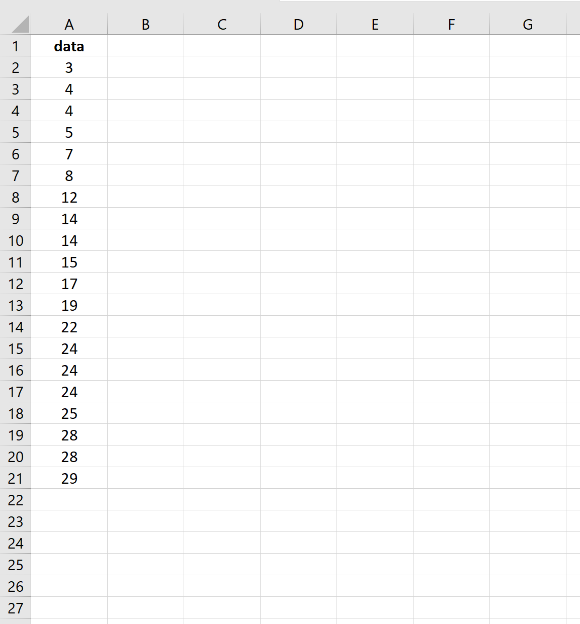
Предположим, у нас есть следующий набор данных:
На следующем снимке экрана показано, как рассчитать стандартную ошибку среднего значения для этого набора данных:
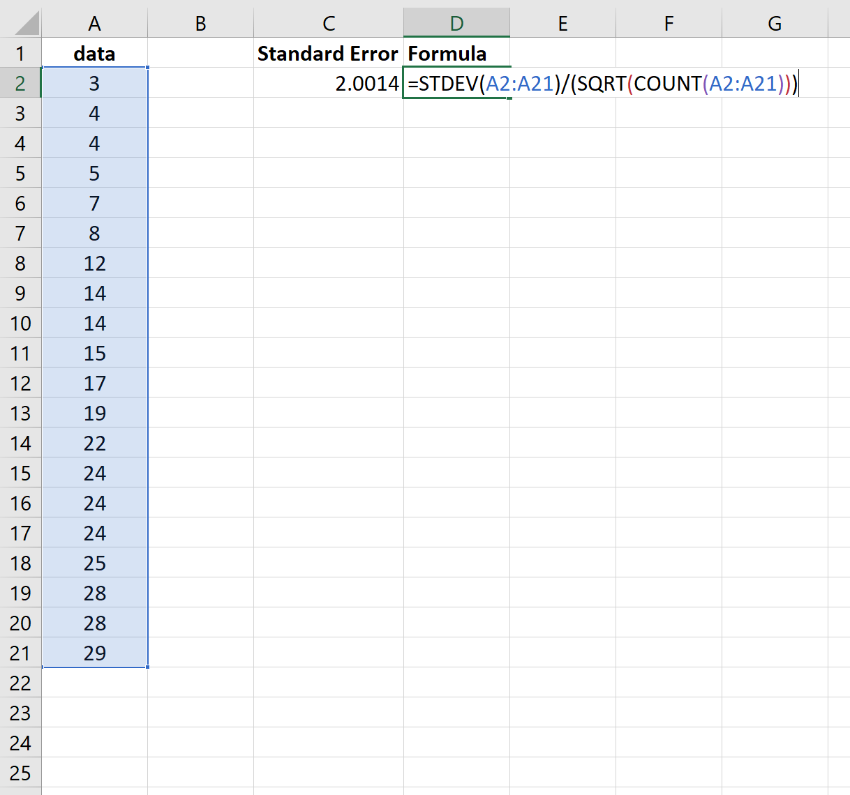
Стандартная ошибка оказывается равной 2,0014 .
Обратите внимание, что функция =СТАНДОТКЛОН() вычисляет выборочное среднее, что эквивалентно функции =СТАНДОТКЛОН.С() в Excel.
Таким образом, мы могли бы использовать следующую формулу для получения тех же результатов:
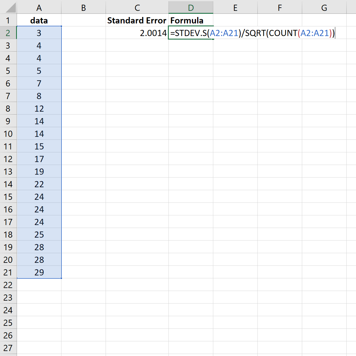
И снова стандартная ошибка оказывается равной 2,0014 .
Как интерпретировать стандартную ошибку среднего
Стандартная ошибка среднего — это просто мера того, насколько разбросаны значения вокруг среднего. При интерпретации стандартной ошибки среднего следует помнить о двух вещах:
1. Чем больше стандартная ошибка среднего, тем более разбросаны значения вокруг среднего в наборе данных.
Чтобы проиллюстрировать это, рассмотрим, изменим ли мы последнее значение в предыдущем наборе данных на гораздо большее число:
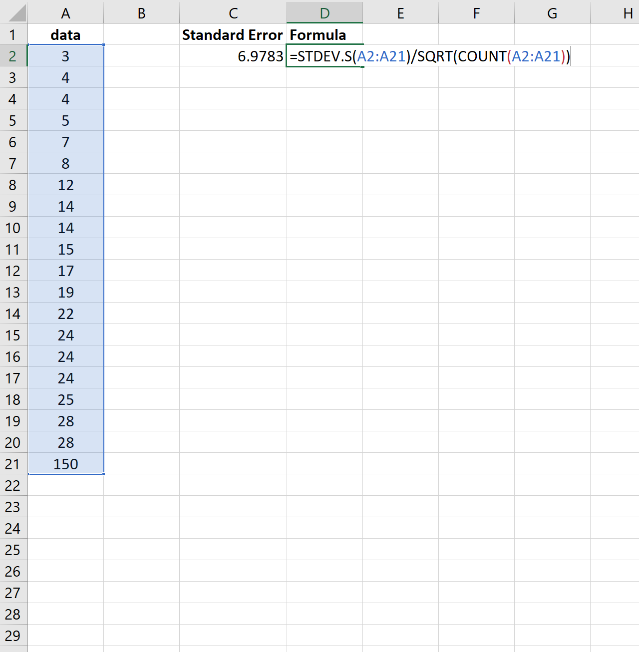
Обратите внимание на скачок стандартной ошибки с 2,0014 до 6,9783.Это указывает на то, что значения в этом наборе данных более разбросаны вокруг среднего значения по сравнению с предыдущим набором данных.
2. По мере увеличения размера выборки стандартная ошибка среднего имеет тенденцию к уменьшению.
Чтобы проиллюстрировать это, рассмотрим стандартную ошибку среднего для следующих двух наборов данных:
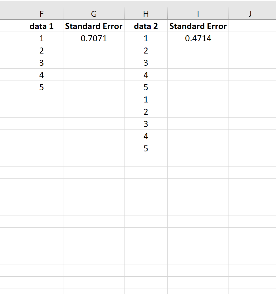
Второй набор данных — это просто первый набор данных, повторенный дважды. Таким образом, два набора данных имеют одинаковое среднее значение, но второй набор данных имеет больший размер выборки, поэтому стандартная ошибка меньше.
Стандартная ошибка появляется при прогнозировании каких-либо данных или арифметических вычислениях, поэтому важно научиться находить этот параметр. В этой публикации разбираем, как найти и исправить стандартную ошибку путем использования инструментов Excel.
Расчет средней арифметической ошибки
В Microsoft Excel цельность и однородность выборки определяется при помощи стандартной ошибки. Стандартная ошибка — это квадратный корень из дисперсии. В приложении предусмотрено два варианта поиска стандартной ошибки: при помощи пакетного анализа и расширенных функций программы.
Чтобы найти значение средней арифметической, необходимо выполнить деление суммарной величины выборки на ее количество в электронной книге.
Расчет стандартной ошибки при помощи встроенных функций
Для того, чтобы правильно вычислять, необходимо изучить пошаговую инструкцию. В этом способе подбор результатов будет осуществляться с помощью комбинированных манипуляций.
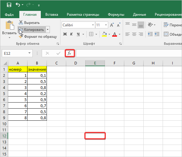
- Для расчетов будем использовать таблицу с выборкой чисел. Кликаем на любой пустой ячейке на листе, где будет отображаться результат. Затем нажимаем кнопку «Вставить функцию.
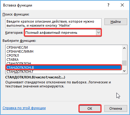
- Далее перед вами открывается диалоговое окно, в котором необходимо использовать «СТАНДОТКЛ.В», для этого в поле «Категория» необходимо выбрать «Полный алфавитный перечень». Затем нажмите кнопку «ОК».
- В окне «Аргументы функции» кликаем в первом поле «Число 1», затем выполняем выделение мышью диапазона ячеек со значениями таблицы и нажимаем кнопку «ОК».
- Далее активируем ячейку с нашими значениями, переходим в строку формулы и ставим после значений наклонную линию. Переходим в поле наименования, кликаем на указывающий вниз флажок, где из списка выбираем «Другие функции».
- Снова активируется окно с перечнем функций, в котором необходимо выбрать категорию «Математические», затем функцию «Корень». Далее нажмите кнопку «ОК».
- Далее открывается окно, в котором необходимо заполнить поле с числом. Для этого переходим в поле «Имя», где спускаемся к пункту «Счет». Если его нет, ищите в дополнительных функциях.
После выполнения этих шагов, стандартная ошибка высчитывается автоматически, пользователю остается только сверить их и проверить значение на некорректное отображение.
Для малых и стандартных выборок необходимо использовать разные формулы. В первом случае (если находится до 30 значений), ее необходимо видоизменить.
Решение задачи с помощью опции «Описательная статистика»
Благодаря опции «Описательная статистика» удается выполнить вычисление по различным критериям. По этим правилам удается найти среднюю арифметическую ошибку. Для использования данного метода предварительно нужно запустить «Пакет анализа».
- Переходим во вкладку «Файл», где перемещаемся в пункт «Параметры». Далее нажимаем на запись «Надстройки».
- Открывается окошко, в нем в графе «Управление» должно быть прописано «Надстройки Excel», затем рядом нажимаем кнопку «Параметры».
- В появившемся окне находим «Пакет анализа» и нажимаем кнопку «ОК».
- Далее выбираем любую свободную ячейку, переходим во вкладку «Данные» и нажимаем «Анализ данных» в блоке «Анализ».

- Происходит запуск вспомогательного окошка, в котором необходимо выбрать из всех инструментов «Описательную статистику» и нажать кнопку «ОК».
- Открывается новый мастер значений. Здесь нужно вводить данные предельно внимательно. В поле «Входной интервал» вносим адрес диапазона ячеек с выборкой. Затем указываем параметр «Группирование» «По столбцам». Затем выбираем место для «выходного интервала», его должно быть столько же, сколько и «входного». Ставим галочку напротив «Итоговая статистика» и нажимаем кнопку «ОК».
В результате вычислений вы получаете небольшую таблицу, в которой указаны все данные с определенной стандартной ошибкой.
Содержание
- Как рассчитать стандартную ошибку среднего в Excel
- Пример: Стандартная ошибка в Excel
- Как интерпретировать стандартную ошибку среднего
- Standard Error Formula
- What is a Standard Error Formula?
- Explanation
- Example of Standard error formula
- Example #1
- Example #2
- Standard Error Calculator
- Relevance and Use
- Standard Error Formula in Excel
- Recommended Articles
- How to Calculate Standard Error in Excel (Step-by-Step)
- What is Standard Error?
- How is Standard Error Calculated?
- How to Find the Standard Error in Excel Using a Formula
- How to Find the Standard Error in Excel Using the Data Analysis Toolpak
- Conclusion
Как рассчитать стандартную ошибку среднего в Excel

Стандартная ошибка среднего — это способ измерить, насколько разбросаны значения в наборе данных. Он рассчитывается как:
Стандартная ошибка = с / √n
- s : стандартное отклонение выборки
- n : размер выборки
Вы можете рассчитать стандартную ошибку среднего для любого набора данных в Excel, используя следующую формулу:
= СТАНДОТКЛОН (диапазон значений) / КОРЕНЬ ( СЧЁТ (диапазон значений))
В следующем примере показано, как использовать эту формулу.
Пример: Стандартная ошибка в Excel
Предположим, у нас есть следующий набор данных:
На следующем снимке экрана показано, как рассчитать стандартную ошибку среднего значения для этого набора данных:
Стандартная ошибка оказывается равной 2,0014 .
Обратите внимание, что функция =СТАНДОТКЛОН() вычисляет выборочное среднее, что эквивалентно функции =СТАНДОТКЛОН.С() в Excel.
Таким образом, мы могли бы использовать следующую формулу для получения тех же результатов:
И снова стандартная ошибка оказывается равной 2,0014 .
Как интерпретировать стандартную ошибку среднего
Стандартная ошибка среднего — это просто мера того, насколько разбросаны значения вокруг среднего. При интерпретации стандартной ошибки среднего следует помнить о двух вещах:
1. Чем больше стандартная ошибка среднего, тем более разбросаны значения вокруг среднего в наборе данных.
Чтобы проиллюстрировать это, рассмотрим, изменим ли мы последнее значение в предыдущем наборе данных на гораздо большее число:
Обратите внимание на скачок стандартной ошибки с 2,0014 до 6,9783.Это указывает на то, что значения в этом наборе данных более разбросаны вокруг среднего значения по сравнению с предыдущим набором данных.
2. По мере увеличения размера выборки стандартная ошибка среднего имеет тенденцию к уменьшению.
Чтобы проиллюстрировать это, рассмотрим стандартную ошибку среднего для следующих двух наборов данных:
Второй набор данных — это просто первый набор данных, повторенный дважды. Таким образом, два набора данных имеют одинаковое среднее значение, но второй набор данных имеет больший размер выборки, поэтому стандартная ошибка меньше.
Источник
Standard Error Formula


What is a Standard Error Formula?
The standard error is the error that arises in the sampling distribution while performing statistical analysis. It is a standard deviation variant as both concepts correspond to the spread measures. A high standard error corresponds to the higher spreading of data for the undertaken sample. Calculating the standard error formula is done for a sample. At the same time, the standard deviation determines the population.
Table of contents
Therefore, a standard error on mean one would express and determine as per the relationship described as follows: –
You are free to use this image on your website, templates, etc., Please provide us with an attribution link How to Provide Attribution? Article Link to be Hyperlinked
For eg:
Source: Standard Error Formula (wallstreetmojo.com)
- The standard error expressed as σ͞x.
- The standard deviation of the population is expressed as σ.
- The number of variables in the sample expressed as n.
Explanation
One can explain the formula for standard error on mean by using the following steps:
- Identify and organize the sample and determine the number of variables.
Next, the average means of the sample corresponds to the number of variables present in the sample.
Next, determine the standard deviation of the sample.
Next, determine the square root of the number of variables taken up in the sample.
Now, divide the standard deviation computed in step 3 by the resulting value in step 4 to arrive at the standard error.
Example of Standard error formula
Below are the formula examples for calculating standard error.
Example #1
Let us take the example of stock ABC. For 30 years, the stock delivered a mean dollar return of $45. In addition, one observed that the stock delivered returns with a standard deviation of $2. Help the investor to calculate the overall standard error on the mean returns offered by the stock ABC.
Solution:
- Standard Deviation (σ) = $2
- Number of Years (n) = 30
- Mean Dollar Return = $45
The calculation of standard error is as follows:
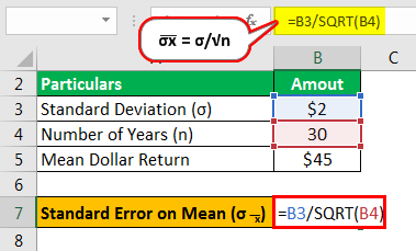
- σ͞x = σ/√n
- = $2/√30
- = $2/ 5.4773
The standard error is,

- σ͞x=$0.3651
Therefore, the investment offers a dollar standard error on the mean of $0.36515 to the investor when holding the stock ABC position for 30 years. However, if the stock held for a higher investment horizon, then the standard error on the dollar means would reduce significantly.
Example #2
Let us take the example of an investor who has received the following returns on stock XYZ: –
| Investment Year | Return Offered |
|---|---|
| 1 | 20% |
| 2 | 25% |
| 3 | 5% |
| 4 | 10% |
Help the investor calculate the overall standard error on the mean returns offered by the stock XYZ.
Solution:
First, determine the average mean of the returns as displayed below: –

- ͞X = (x1+x2+x3+x4)/number of years
- = (20+25+5+10)/4
- =15%
Now, determine the standard deviation of the returns as displayed below: –
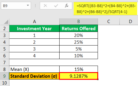
- σ = √ ((x1-͞X) 2 + (x2-͞X) 2 + (x3-͞X) 2 + (x4-͞X) 2 ) / √ (number of years -1)
- = √ ((20-15) 2 + (25-15) 2 + (5-15) 2 + (10-15) 2 ) / √ (4-1)
- = (√ (5) 2 + (10) 2 + (-10) 2 + (-5) 2 ) / √ (3)
- = (√25+100+100+25)/ √ (3)
- =√250 /√ 3
- =√83.3333
- = 9.1287%
Now, the calculation of standard error is as follows,

- σ͞x = σ/√n
- = 9.128709/√4
- = 9.128709/ 2
The standard Error is,

- σ͞x= 4.56%
Therefore, the investment offers a dollar standard error on the mean of 4.56% to the investor when holding the stock XYZ position for 4 years.
Standard Error Calculator
You can use the following calculator.
| σ |
| n |
| Standard Error Formula |
Relevance and Use
The standard error tends to be high if the sample size for the analysis is small. Therefore, a sample is always taken from a larger population, which comprises a larger size of variables. It always helps the statistician determine the sample mean’s credibility concerning the population mean.
A large standard error tells the statistician that the sample is not uniform concerning the population mean. There is a large variation in the sample concerning the population. Similarly, a small standard error tells the statistician that the sample is uniform concerning the population mean. There is no or small variation in the sample concerning the population.
Standard Error Formula in Excel
Now, let us take the excel example to illustrate the concept of the standard error formula in the Excel template below. Suppose the school administration wants to determine the standard error on mean on the height of the football players.
The sample comprises of following values: –

Help the administration assess standard error on mean.
Step 1: Determine the mean as displayed below: –

Step 2: Determine the standard deviation as displayed below: –

Step 3: Determine the standard error on mean as displayed below: –

Therefore, the standard error on the mean for football players is 1.846 inches. The management should observe that it is significantly large. Therefore, the sample data taken up for the analysis is not uniform and displays a large variance.
The management should either omit smaller players or add significantly taller players to balance the football team’s average height by replacing them with individuals with smaller heights compared to their peers.
Recommended Articles
This article has been a guide to Standard Error Formula. Here, we discuss the formula for calculating the mean, standard error, examples, and downloadable Excel sheet. You can learn more from the following articles: –
Источник
How to Calculate Standard Error in Excel (Step-by-Step)
Most people use spreadsheets software such as Microsoft Excel to process their data and carry out their analysis tasks.
When performing an analysis of data, a number of statistical metrics come into play. Some of these include the means, the medians, standard deviations, and standard errors. These metrics help in understanding the true nature of the data.
In this article, I will show you two ways to calculate the Standard Error in Excel.
One of the methods involves using a formula and the other involves using a Data Analytics Tool Pack that usually comes with every copy of Excel.
So let’s get started!
Table of Contents
What is Standard Error?
When working with real-world data, it is often not possible to work with data of the entire population. So we usually take random samples from the population and work with them.
The standard error of a sample tells how accurate its mean is in terms of the true population mean.
In other words, the standard error of a sample is its standard deviation from the population mean.
This helps analyze how accurately your sample’s mean represents the true population. It also helps analyze the amount of dispersion or variation between your different data samples.
How is Standard Error Calculated?
The Standard Error for a sample is usually calculated using the formula:
In this above formula:
- SE is Standard Error
- σ represents the Standard deviation of the sample
- n represents the sample size.
How to Find the Standard Error in Excel Using a Formula
Unfortunately, unlike the Standard Deviation, Excel does not have a built-in formula to calculate the Standard Error, at least not at the time of writing this tutorial.
However, you could use the above formula to easily and quickly calculate the standard error. Here are the steps you need to follow:
- Click on the cell where you want the Standard Error to appear and click on the formula bar next to the fx symbol just below your toolbar.
- Type the symbol ‘=’ in the formula bar. And type: =STDEV(
- Drag and select the range of cells that are part of your sample data. This will add the location of the range in your formula. So, if your sample data is in cells B2 to B14, you will see: =STDEV(B2:B14 in the formula bar.
- Close the bracket for the STDEV formula. So far, you have used the STDEV function to find the Standard deviation of your sample data.
- Next, we want to divide this Standard deviation by the square root of the sample size. So let’s continue with our formula. Click on the formula bar after the closing brackets of the STDEV formula and add a ‘/’ symbol to indicate that you want to divide the result of the STDEV function. So your formula so far is: =STDEV(B2:B14)/
- To find the square root of a number, we use the SQRT formula. So next, type SQRT(. Your formula bar will now have the formula: =STDEV(B2:B14)/SQRT(
- Finally, you want the sample size. For this, you need to use the COUNT function. So, type COUNT( after what you already have in your formula bar. Again, drag and select the range of cells that are part of your sample data and close the bracket for the COUNT formula. This will give you the number of cells in your selected range.
- Close the bracket for the SQRT function too. So your final formula should look like this: =STDEV(B2:B14)/SQRT(COUNT(B2:B14)) Notice there are two closing braces in the end. One is for the COUNT function, the other is for the SQRT function.
- That’s it! Press the return key on your keyboard and you got your sample’s Standard Error!
To find the Standard errors for the other samples, you can apply the same formula to these samples too.
If your samples are placed in columns adjacent to one another (as shown in the above image), you only need to drag the fill handle (located at the bottom left corner of your calculated cell) to the right.
This will copy the same formula to all the other cells on the right, and you will get standard errors for each of your samples!
How to Find the Standard Error in Excel Using the Data Analysis Toolpak
If you’re not in the mood to type complex formulae, there’s an easier way to find not just the Standard error, but practically all the statistical metrics you might need to analyze your sample data.
For this, you will need to install the Data Analysis Toolpak. This package gives you access to a variety of statistical functions, which include correlation functions, z-test, and t-test functions too.
Once you install the package, you can use the tool whenever you need to analyze data, without having to re-install it each time.
The Data Analysis Toolpak is free to use and comes along with your Excel package, but for simplicity, it does not appear in your standard toolbar. You need to activate it in order for it to be added to your toolbar.
The process of activating it is quite simple. Just follow these steps to install and activate your Data Analysis Toolpak:
- Click the File tab and click on Options. This will open the Options window for you.
- From here, click “Add-ins” from the left sidebar.
- From the list of Add-ins, select Analysis ToolPak.
- At the bottom of the window, click on the ‘Go’ button just next to Manage: Add-ins.
- Click the checkmark for Analysis ToolPak and click OK.
With this, your Data Analysis Toolpak will get added to your Excel Toolbar. When you click the Excel ‘Data’ tab, you should find a tool named “Data Analysis” at the far right of the Data toolbar (under the ‘Analysis’ group).
Now, to find out your Standard Error and other Statistical metrics, do the following:
- Click on the Data Analysis tool under the Data tab. This will open the Analysis Tools dialog box.
- Select “Descriptive Statistics” from the list on the left of the dialog box and click OK.
- Enter the location of the range of cells that contain your sample data into the “Input Range” box. You can also choose to drag and select the range of cells that you need too. If you have data for more than one sample arranged in adjacent columns, you can select the data in all the columns. You will get your results separately for each column.
- If your data has column headers, check the “Labels in first row” box.
- Select where you want your results to be displayed. It is safer to select “New Worksheet”. This will ensure that the details get displayed on a newly created worksheet, and will not disturb any data on your current worksheet.
- Select the checkbox next to “Summary Statistics” and click OK.
This will display all your analytical metrics in a new worksheet.
These metrics will also include the Standard Error for your selected sample data. If you had selected multiple data sets in multiple columns, you will get analytics for each column separately.
Conclusion
In this article, we discussed two ways in which you can find the Standard error for your sample data.
You can either create a formula to calculate it or use a data analytics tool, like the Data Analysis Toolpak that comes with Excel.
Either way, you will be able to use the Standard error information to analyze your sample data for further processing.
Hope you found this Excel tutorial useful!
Other Excel tutorials you may find useful:
Источник
Excel для Microsoft 365 Excel для Microsoft 365 для Mac Excel для Интернета Excel 2021 Excel 2021 for Mac Excel 2019 Excel 2019 для Mac Excel 2016 Excel 2016 для Mac Excel 2013 Excel 2010 Excel 2007 Excel для Mac 2011 Excel Starter 2010 Еще…Меньше
В этой статье описаны синтаксис формулы и использование функции СТОШYX в Microsoft Excel.
Описание
Возвращает стандартную ошибку предсказанных значений y для каждого значения x в регрессии. Стандартная ошибка — это мера ошибки предсказанного значения y для отдельного значения x.
Синтаксис
СТОШYX(известные_значения_y;известные_значения_x)
Аргументы функции СТОШYX описаны ниже.
-
Известные_значения_y Обязательный. Массив или диапазон зависимых точек данных.
-
Известные_значения_x Обязательный. Массив или диапазон независимых точек данных.
Замечания
-
Аргументы могут быть либо числами, либо содержащими числа именами, массивами или ссылками.
-
Учитываются логические значения и текстовые представления чисел, которые непосредственно введены в список аргументов.
-
Если аргумент, который является массивом или ссылкой, содержит текст, логические значения или пустые ячейки, то такие значения пропускаются; однако ячейки, которые содержат нулевые значения, учитываются.
-
Аргументы, которые представляют собой значения ошибок или текст, не преобразуемый в числа, вызывают ошибку.
-
Если аргументы «известные_значения_y» и «известные_значения_x» содержат различное количество точек данных, то функция СТОШYX возвращает значение ошибки #Н/Д.
-
Если known_y и known_x пустые или имеют менее трех точек данных, steYX возвращает #DIV/0! значение ошибки #ЗНАЧ!.
-
Уравнение для стандартной ошибки предсказанного y имеет следующий вид:
где x и y — выборочные средние значения СРЗНАЧ(известные_значения_x) и СРЗНАЧ(известные_значения_y), а n — размер выборки.
Пример
Скопируйте образец данных из следующей таблицы и вставьте их в ячейку A1 нового листа Excel. Чтобы отобразить результаты формул, выделите их и нажмите клавишу F2, а затем — клавишу ВВОД. При необходимости измените ширину столбцов, чтобы видеть все данные.
|
Данные |
||
|
Известные значения y |
Известные значения x |
|
|
2 |
6 |
|
|
3 |
5 |
|
|
9 |
11 |
|
|
1 |
7 |
|
|
8 |
5 |
|
|
7 |
4 |
|
|
5 |
4 |
|
|
Формула |
Описание (результат) |
Результат |
|
=СТОШYX(A3:A9;B3:B9) |
Стандартная ошибка предсказанных значений y для каждого значения x в регрессии (3,305719) |
3,305719 |
Нужна дополнительная помощь?
What is a Standard Error Formula?
The standard error is the error that arises in the sampling distribution while performing statistical analysis. It is a standard deviation variant as both concepts correspond to the spread measures. A high standard error corresponds to the higher spreading of data for the undertaken sample. Calculating the standard error formula is done for a sample. At the same time, the standard deviation determines the population.
Table of contents
- What is a Standard Error Formula?
- Explanation
- Example of Standard error formula
- Standard Error Calculator
- Relevance and Use
- Standard Error Formula in Excel
- Recommended Articles
Therefore, a standard error on mean one would express and determine as per the relationship described as follows: –
σ͞x = σ/√n
You are free to use this image on your website, templates, etc., Please provide us with an attribution linkArticle Link to be Hyperlinked
For eg:
Source: Standard Error Formula (wallstreetmojo.com)
Here,
- The standard error expressed as σ͞x.
- The standard deviation of the population is expressed as σ.
- The number of variables in the sample expressed as n.
In statistical analysis, mean, median, and mode are central tendencyCentral Tendency is a statistical measure that displays the centre point of the entire Data Distribution & you can find it using 3 different measures, i.e., Mean, Median, & Mode.read more measures. The standard deviation, variance, and standard error on mean classifies as the variability measures. The standard error on mean for sample data is directly related to the standard deviation of the larger population and inversely proportional or related to the square rootThe Square Root function is an arithmetic function built into Excel that is used to determine the square root of a given number. To use this function, type the term =SQRT and hit the tab key, which will bring up the SQRT function. Moreover, this function accepts a single argument.read more of several variables taken up for making a sample. Hence, if the sample sizeThe sample size formula depicts the relevant population range on which an experiment or survey is conducted. It is measured using the population size, the critical value of normal distribution at the required confidence level, sample proportion and margin of error.read more is small, then there could be an equal probability that the standard error would also be large.
Explanation
One can explain the formula for standard error on mean by using the following steps:
- Identify and organize the sample and determine the number of variables.
- Next, the average means of the sample corresponds to the number of variables present in the sample.
- Next, determine the standard deviation of the sample.
- Next, determine the square root of the number of variables taken up in the sample.
- Now, divide the standard deviation computed in step 3 by the resulting value in step 4 to arrive at the standard error.
Example of Standard error formula
Below are the formula examples for calculating standard error.
You can download this Standard Error Formula Excel Template here – Standard Error Formula Excel Template
Example #1
Let us take the example of stock ABC. For 30 years, the stock delivered a mean dollar return of $45. In addition, one observed that the stock delivered returns with a standard deviation of $2. Help the investor to calculate the overall standard error on the mean returns offered by the stock ABC.
Solution:
- Standard Deviation (σ) = $2
- Number of Years (n) = 30
- Mean Dollar Return = $45
The calculation of standard error is as follows:
- σ͞x = σ/√n
- = $2/√30
- = $2/ 5.4773
The standard error is,
- σ͞x =$0.3651
Therefore, the investment offers a dollar standard error on the mean of $0.36515 to the investor when holding the stock ABC position for 30 years. However, if the stock held for a higher investment horizon, then the standard error on the dollar means would reduce significantly.
Example #2
Let us take the example of an investor who has received the following returns on stock XYZ: –
| Investment Year | Return Offered |
|---|---|
| 1 | 20% |
| 2 | 25% |
| 3 | 5% |
| 4 | 10% |
Help the investor calculate the overall standard error on the mean returns offered by the stock XYZ.
Solution:
First, determine the average mean of the returns as displayed below: –
- ͞X = (x1+x2+x3+x4)/number of years
- = (20+25+5+10)/4
- =15%
Now, determine the standard deviation of the returns as displayed below: –
- σ = √ ((x1-͞X)2 + (x2-͞X)2 + (x3-͞X)2 + (x4-͞X)2) / √ (number of years -1)
- = √ ((20-15) 2 + (25-15) 2 + (5-15) 2 + (10-15) 2) / √ (4-1)
- = (√ (5) 2 + (10) 2 + (-10) 2 + (-5) 2 ) / √ (3)
- = (√25+100+100+25)/ √ (3)
- =√250 /√ 3
- =√83.3333
- = 9.1287%
Now, the calculation of standard error is as follows,
- σ͞x = σ/√n
- = 9.128709/√4
- = 9.128709/ 2
The standard Error is,
- σ͞x = 4.56%
Therefore, the investment offers a dollar standard error on the mean of 4.56% to the investor when holding the stock XYZ position for 4 years.
Standard Error Calculator
You can use the following calculator.
| σ | |
| n | |
| Standard Error Formula | |
Relevance and Use
The standard error tends to be high if the sample size for the analysis is small. Therefore, a sample is always taken from a larger population, which comprises a larger size of variables. It always helps the statistician determine the sample mean’s credibility concerning the population mean.
A large standard error tells the statistician that the sample is not uniform concerning the population mean. There is a large variation in the sample concerning the population. Similarly, a small standard error tells the statistician that the sample is uniform concerning the population mean. There is no or small variation in the sample concerning the population.
One should not mix it with the standard deviation. Instead, one should calculate the standard deviation for the entire population. The standard errorStandard Error (SE) is a metric that measures the accuracy of a sample distribution that signifies a population by using standard deviation. In other words, it is a measure to the dispersion of a sample mean concerned with the population mean and is not standard deviation.read more, on the other hand, is determined for the sample mean.
Standard Error Formula in Excel
Now, let us take the excel example to illustrate the concept of the standard error formula in the Excel template below. Suppose the school administration wants to determine the standard error on mean on the height of the football players.
The sample comprises of following values: –
Help the administration assess standard error on mean.
Step 1: Determine the mean as displayed below: –
Step 2: Determine the standard deviation as displayed below: –
Step 3: Determine the standard error on mean as displayed below: –
Therefore, the standard error on the mean for football players is 1.846 inches. The management should observe that it is significantly large. Therefore, the sample data taken up for the analysis is not uniform and displays a large variance.
The management should either omit smaller players or add significantly taller players to balance the football team’s average height by replacing them with individuals with smaller heights compared to their peers.
Recommended Articles
This article has been a guide to Standard Error Formula. Here, we discuss the formula for calculating the mean, standard error, examples, and downloadable Excel sheet. You can learn more from the following articles: –
- EBITDA Margin Formula
- Gross Margin Formula
- Formula of Relative Standard Deviation
- Formula of Margin of Error