How are the standard errors and confidence intervals computed for
relative-risk ratios (RRRs) by mlogit?
How are the standard errors and confidence intervals computed for
odds ratios (ORs) by logistic?
How are the standard errors and confidence intervals computed for
incidence-rate ratios (IRRs) by poisson
and nbreg?
How are the standard errors and confidence intervals computed for
hazard ratios (HRs) by stcox and
streg?
| Title | Standard errors, confidence intervals, and significance tests for ORs, HRs, IRRs, and RRRs | |
| Authors | William Sribney, StataCorp Vince Wiggins, StataCorp |
Question:
How does Stata get the standard errors of the odds ratios reported by
logistic and why do the reported confidence intervals not agree with a 95%
confidence bound on the reported odds ratio using these standard errors?
Likewise, why does the reported significance test of the odds ratio not
agree with either a test of the odds ratio against 0 or a test against 1
using the reported standard error?
Standard Errors
The odds ratios (ORs), hazard ratios (HRs), incidence-rate ratios (IRRs),
and relative-risk ratios (RRRs) are all just univariate transformations of
the estimated betas for the logistic, survival, and multinomial logistic
models. Using the odds ratio as an example, for any coefficient b we have
ORb = exp(b)
When ORs (or HRs, or IRRs, or RRRs) are reported, Stata uses the
delta rule to derive an estimate of the
standard error of ORb. For the simple expression of
ORb, the standard error by the delta rule is just
se(ORb) = exp(b)*se(b)
Confidence intervals—short answer
The confidence intervals reported by Stata for the odds ratios are the exp()
transformed endpoints of the confidence intervals in the natural parameter
space—the betas. They are
        CI(ORb) = [exp(bL), exp(bU)]

               where:
                     bL = lower limit of confidence interval for b
                     bU = upper limit of confidence interval for b
Here is an example with logistic. We show how to obtain the standard
errors and confidence intervals for odds ratios manually in Stata’s method
. webuse lbw, clear
 (Hosmer & Lemeshow data)

. logistic low age lwt i.race smoke, coef

Logistic regression                             Number of obs     =        189
                                                LR chi2(5)        =      20.08
                                                Prob > chi2       =     0.0012
Log likelihood = -107.29639                     Pseudo R2         =     0.0856
| low | Odds Ratio Std. Err. z P>|z| [95% Conf. Interval] | |
| age | -.0225071 .0341688 -0.66 0.510 -.0894766 .0444625 | |
| lwt | -.0125017 .0063843 -1.96 0.050 -.0250146 .0000113 | |
| race | ||
| black | 1.23121 .5171062 2.38 0.017 .2177006 2.244719 | |
| other | .9435946 .4162001 2.27 0.023 .1278573 1.759332 | |
| smoke | 1.054433 .3799787 2.77 0.006 .3096879 1.799177 | |
| _cons | .3301267 1.107607 0.30 0.766 -1.840743 2.500997 | |
| low | Odds Ratio Std. Err. z P>|z| [95% Conf. Interval] | |
| age | .9777443 .0334083 -0.66 0.510 .9144097 1.045466 | |
| lwt | .9875761 .006305 -1.96 0.050 .9752956 1.000011 | |
| race | ||
| black | 3.425372 1.771281 2.38 0.017 1.243215 9.437768 | |
| other | 2.5692 1.069301 2.27 0.023 1.136391 5.808555 | |
| smoke | 2.870346 1.09067 2.77 0.006 1.363 6.044672 | |
| _cons | 1.391144 1.540841 0.30 0.766 .1586994 12.19464 | |
Some people prefer confidence intervals computed from the odds-ratio
estimates and the delta rule SEs. Asymptotically, these two are equivalent,
but they will differ for real data.
In practice, the confidence intervals obtained by transforming the endpoints
have some intuitively desirable properties; e.g., they do not produce
negative odds ratios. In general, we also expect the estimates to be more
normally distributed in the natural space of the problem (the beta space);
see the long answer below.
Test of significance
The proper test of significance for ORs, HRs, IRRs, and RRRs is whether the
ratio is 1 not whether the ratio is 0. The test against 0 is a test that
the coefficient for the parameter in the fitted model is negative infinity
and has little meaning. Stata reports the test of whether the ratio (OR,
HR, IRR, RRR) differs from 1—e.g., H0: ORb = 1.
As with the confidence interval, there are two asymptotically equivalent
ways to form this test: (1) Test whether the parameter b differs from 0 in
the natural space of the model (H0: b = 0), or (2) test whether the
transformed parameter differs from 1 in the OR space (H0: exp(b) = 1). The
latter test would use the SE(ORb) from the delta rule. When
reporting ORs, HRs, or RRRs, Stata reports the statistic and significance
level from the test in the natural estimation space—H0: b = 0.
Asymptotic theory gives no clue as to which test should be preferred, but we
would expect the estimates to be more normally distributed in the natural
estimation space—see the discussion below.
Confidence intervals (CIs)—long answer
To continue with the point that confidence intervals can be computed in two
ways for transformed estimates (ORs, RRRs, IRRs, HRs, …), a user asked
Wouldn’t it be more appropriate to use the the standard errors for the
RR when calculating CI?
Asymptotically, both methods are equally valid, but it is better to
start with the CI in the metric in which the estimates are closer to normal
and then transform its endpoints. Since the estimate b is likely to be more
normal than exp(b) (since exp(b) is likely to be skewed), it is better to
transform the endpoints of the CI for b to produce a CI for exp(b).
First, when you transform a standard error of an ML estimate using the delta
method, you get the same standard error that you would have obtained had you
performed the maximization with the transformed parameter directly.
Consider a general transformation B = f(b) of b. Using the delta method,
Var(B) = f'(b)2 * Var(b) = f'(b)2 * (d2 lnL/db2)-1
where lnL is the log likelihood. Had we done the maximization in B,
     d ln L/dB = d lnL/db * db/dB

     d2 lnL/dB2 = d2 lnL/db2 * (db/dB)2 + d lnL/db * d2b/dB2
since d lnL/db = 0 at the maximum,
d2 lnL/dB2 = d2 lnL/db2 * (db/dB)2 = d2 lnL/db2 * f'(b)-2
hence,
Var(B) = (d2 lnL/dB2)-1 = (d2 lnL/db2)-1 * f'(b)2
So this fact might give someone more reason to say we should use the
standard error of B to produce its CI.
However, we could also use this as evidence to say we could use ANY
transformation to produce a confidence interval. That is, we could look at
further transformations g(B) of B. According to asymptotic theory,
[g(B) - z*se(g(B)), g(B) + z*se(g(B))] (1)
gives a valid CI for g(B) (where z is the normal quantile and se(g(B)) is
the standard error computed using the delta method).
This CI with endpoints transformed back to the B metric gives a CI
[g-1(g(B) - z*se(g(B))), g-1(g(B) + z*se(g(B)))]
The above CI must give an equally valid CI since it will yield the same
coverage probability as (1).
So, ideally, we should search for the best transformation g(B) of any
quantity B such that g(B) is roughly normal so that the CI given above gives
the best coverage probability.
The estimate B = exp(b) is likely to have a skewed distribution, so
it is certainly not likely to be as normal as the distribution of the
coefficient estimate b. It’s better to use g = exp−1
to produce the CI for B = exp(b).
Both CIs are equally valid according to asymptotic theory. But, in
practice, the CI produced from the more normal estimate (i.e., b rather than
exp(b)) will likely yield slightly better CIs for coverage probability.
Multiple linear regression is a method we can use to understand the relationship between several explanatory variables and a response variable.
Unfortunately, one problem that often occurs in regression is known as heteroscedasticity, in which there is a systematic change in the variance of residuals over a range of measured values.
This causes an increase in the variance of the regression coefficient estimates, but the regression model doesn’t pick up on this. This makes it much more likely for a regression model to declare that a term in the model is statistically significant, when in fact it is not.
One way to account for this problem is to use robust standard errors, which are more “robust” to the problem of heteroscedasticity and tend to provide a more accurate measure of the true standard error of a regression coefficient.
This tutorial explains how to use robust standard errors in regression analysis in Stata.
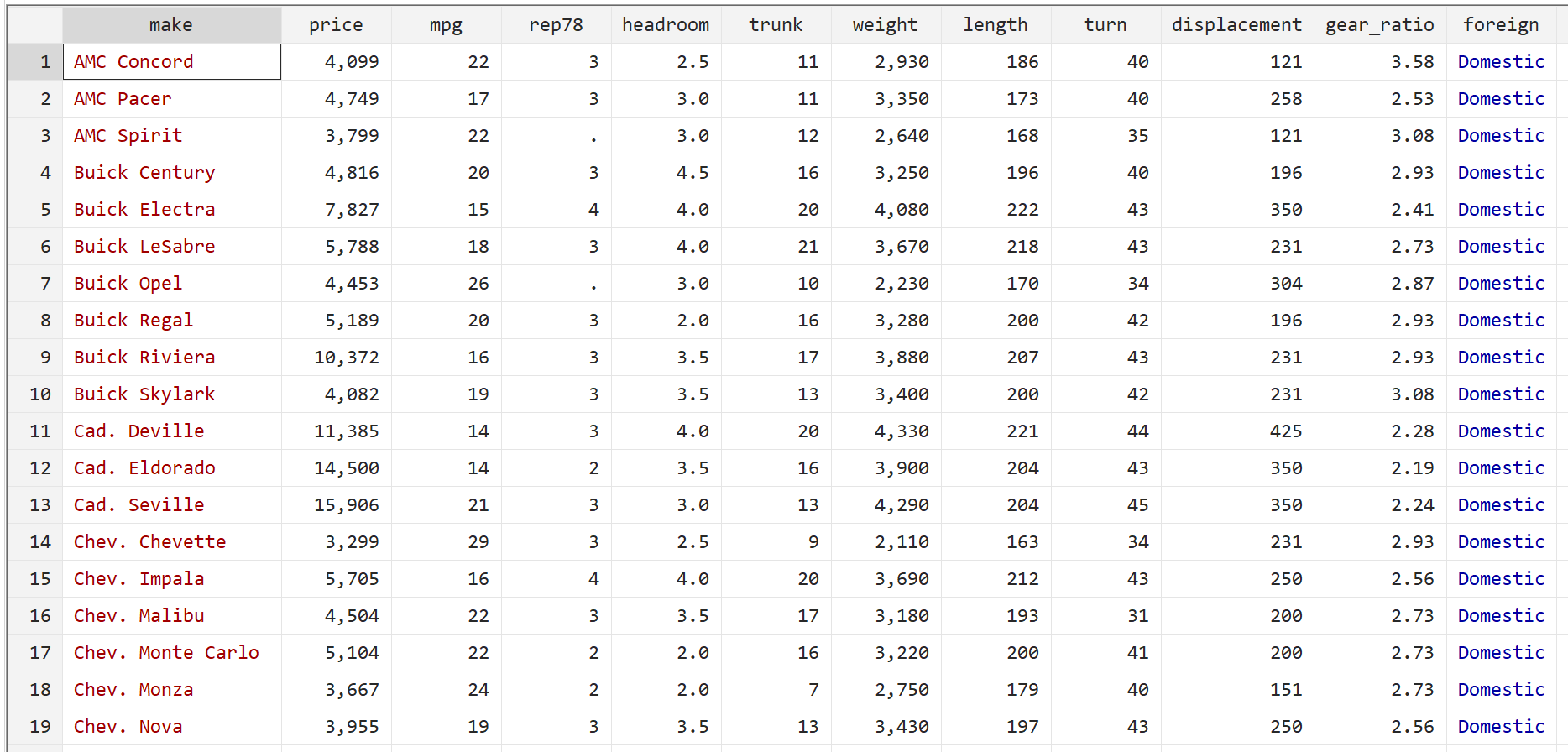
We will use the built-in Stata dataset auto to illustrate how to use robust standard errors in regression.
Step 1: Load and view the data.
First, use the following command to load the data:
sysuse auto
Then, view the raw data by using the following command:
br

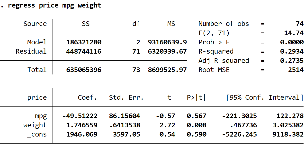
Step 2: Perform multiple linear regression without robust standard errors.
Next, we will type in the following command to perform a multiple linear regression using price as the response variable and mpg and weight as the explanatory variables:
regress price mpg weight

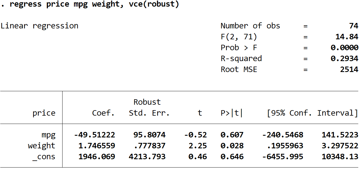
Step 3: Perform multiple linear regression using robust standard errors.
Now we will perform the exact same multiple linear regression, but this time we’ll use the vce(robust) command so Stata knows to use robust standard errors:
regress price mpg weight, vce(robust)

There are a few interesting things to note here:
1. The coefficient estimates remained the same. When we use robust standard errors, the coefficient estimates don’t change at all. Notice that the coefficient estimates for mpg, weight, and the constant are as follows for both regressions:
- mpg: -49.51222
- weight: 1.746559
- _cons: 1946.069
2. The standard errors changed. Notice that when we used robust standard errors, the standard errors for each of the coefficient estimates increased.
Note: In most cases, robust standard errors will be larger than the normal standard errors, but in rare cases it is possible for the robust standard errors to actually be smaller.
3. The test statistic of each coefficient changed. Notice that the absolute value of each test statistic, t, decreased. This is because the test statistic is calculated as the estimated coefficient divided by the standard error. Thus, the larger the standard error, the smaller the absolute value of the test statistic.
4. The p-values changed. Notice that the p-values for each variable also increased. This is because smaller test statistics are associated with larger p-values.
Although the p-values changed for our coefficients, the variable mpg is still not statistically significant at α = 0.05 and the variable weight is still statistically significant at α = 0.05.
What are robust standard errors? How do we calculate them? Why use them? Why not use them all the time if they’re so robust? Those are the kinds of questions this post intends to address.
To begin, let’s start with the relatively easy part: getting robust standard errors for basic linear models in Stata and R. In Stata, simply appending vce(robust) to the end of regression syntax returns robust standard errors. “vce” is short for “variance-covariance matrix of the estimators”. “robust” indicates which type of variance-covariance matrix to calculate. Here’s a quick example using the auto data set that comes with Stata 16:
. sysuse auto
(1978 Automobile Data)

. regress mpg turn trunk, vce(robust)

Linear regression                               Number of obs     =         74
                                                F(2, 71)          =      68.76
                                                Prob > F          =     0.0000
                                                R-squared         =     0.5521
                                                Root MSE          =      3.926

------------------------------------------------------------------------------
             |               Robust
         mpg |      Coef.   Std. Err.      t    P>|t|     [95% Conf. Interval]
-------------+----------------------------------------------------------------
        turn |  -.7610113   .1447766    -5.26   0.000    -1.049688    -.472335
       trunk |  -.3161825   .1229278    -2.57   0.012    -.5612936   -.0710714
       _cons |   55.82001   4.866346    11.47   0.000     46.11679    65.52323
Notice the third column indicates “Robust” Standard Errors.
To replicate the result in R takes a bit more work. First we load the haven package to use the read_dta function that allows us to import Stata data sets. Then we load two more packages: lmtest and sandwich. The lmtest package provides the coeftest function that allows us to re-calculate a coefficient table using a different variance-covariance matrix. The sandwich package provides the vcovHC function that allows us to calculate robust standard errors. The type argument allows us to specify what kind of robust standard errors to calculate. “HC1” is one of several types available in the sandwich package and happens to be the default type in Stata 16. (We talk more about the different types and why it’s called the “sandwich” package below.)
library(haven)
library(lmtest)
library(sandwich)

auto <- read_dta('http://www.stata-press.com/data/r16/auto.dta')
m <- lm(mpg ~ turn + trunk, data = auto)
coeftest(m, vcov. = vcovHC(m, type = 'HC1'))

##
## t test of coefficients:
##
##             Estimate Std. Error t value  Pr(>|t|)
## (Intercept) 55.82001    4.86635 11.4706 < 2.2e-16 ***
## turn        -0.76101    0.14478 -5.2565 1.477e-06 ***
## trunk       -0.31618    0.12293 -2.5721    0.0122 *
## ---
## Signif. codes:  0 '***' 0.001 '**' 0.01 '*' 0.05 '.' 0.1 ' ' 1
If you look carefully you’ll notice the standard errors in the R output match those in the Stata output.
If we want 95% confidence intervals like those produced in Stata, we need to use the coefci function:
coefci(m, vcov. = vcovHC(m, type = 'HC1'))

##                  2.5 %      97.5 %
## (Intercept) 46.1167933 65.52322937
## turn        -1.0496876 -0.47233499
## trunk       -0.5612936 -0.07107136
While not really the point of this post, we should note the results say that larger turn circles and bigger trunks are associated with lower gas mileage.
Now that we know the basics of getting robust standard errors out of Stata and R, let’s talk a little about why they’re robust by exploring how they’re calculated.
The usual method for estimating coefficient standard errors of a linear model can be expressed with this somewhat intimidating formula:
[text{Var}(hat{beta}) = (X^TX)^{-1} X^TOmega X (X^TX)^{-1}] where (X) is the model matrix (ie, the matrix of the predictor values) and (Omega = sigma^2 I_n), which is shorthand for a matrix with nothing but (sigma^2) on the diagonal and 0’s everywhere else. Two main things to notice about this equation:
- The (X^T Omega X) in the middle
- The ((X^TX)^{-1}) on each side
Some statisticians and econometricians refer to this formula as a “sandwich” because it’s like an equation sandwich: we have “meat” in the middle, (X^T Omega X), and “bread” on the outside, ((X^TX)^{-1}). Calculating robust standard errors means substituting a new kind of “meat”.
Before we do that, let’s use this formula by hand to see how it works when we calculate the usual standard errors. This will give us some insight to the meat of the sandwich. To make this easier to demonstrate, we’ll use a small toy data set.
set.seed(1)
x <- c(1:4, 7)
y <- c(5 + rnorm(4,sd = 1.2), 35)
plot(x, y)

Notice the way we generated y. It is simply the number 5 with some random noise from a N(0,1.2) distribution plus the number 35. There is no relationship between x and y. However, when we regress y on x using lm we get a slope coefficient of about 5.2 that appears to be “significant”.
m <- lm(y ~ x)
summary(m)

##
## Call:
## lm(formula = y ~ x)
##
## Residuals:
##      1      2      3      4      5
##  5.743  1.478 -4.984 -7.304  5.067
##
## Coefficients:
##             Estimate Std. Error t value Pr(>|t|)
## (Intercept)   -6.733      5.877  -1.146   0.3350
## x              5.238      1.479   3.543   0.0383 *
## ---
## Signif. codes:  0 '***' 0.001 '**' 0.01 '*' 0.05 '.' 0.1 ' ' 1
##
## Residual standard error: 6.808 on 3 degrees of freedom
## Multiple R-squared:  0.8071, Adjusted R-squared:  0.7428
## F-statistic: 12.55 on 1 and 3 DF,  p-value: 0.03829
Clearly the 5th data point is highly influential and driving the “statistical significance”, which might lead us to think we have specified a “correct” model. Of course we know that we specified a “wrong” model because we generated the data. y does not have a relationship with x! It would be nice if we could guard against this sort of thing from happening: specifying a wrong model but getting a statistically significant result. One way we could do that is modifying how the coefficient standard errors are calculated.
Let’s see how they were calculated in this case using the formula we specified above. Below s2 is (sigma^2), diag(5) is (I_n), and X is the model matrix. Notice we can use the base R function model.matrix to get the model matrix from a fitted model. We save the formula result into vce, which is the variance-covariance matrix. Finally we take square root of the diagonal elements to get the standard errors output in the model summary.
s2 <- sigma(m)^2
X <- model.matrix(m)
vce <- solve(t(X) %*% X) %*% (t(X) %*% (s2*diag(5)) %*% X) %*% solve(t(X) %*% X)
sqrt(diag(vce))

## (Intercept)           x
##    5.877150    1.478557
Now let’s take a closer look at the “meat” in this sandwich formula:
s2*diag(5)

##        [,1]   [,2]   [,3]   [,4]   [,5]
## [1,] 46.346  0.000  0.000  0.000  0.000
## [2,]  0.000 46.346  0.000  0.000  0.000
## [3,]  0.000  0.000 46.346  0.000  0.000
## [4,]  0.000  0.000  0.000 46.346  0.000
## [5,]  0.000  0.000  0.000  0.000 46.346
That is a matrix of constant variance. This is one of the assumptions of classic linear modeling: the errors (or residuals) are drawn from a single Normal distribution with mean 0 and a fixed variance. The s2 object above is the estimated variance of that Normal distribution. But what if we modified this matrix so that the variance was different for some observations? For example, it might make sense to assume the error of the 5th data point was drawn from a Normal distribution with a larger variance. This would result in a larger standard error for the slope coefficient, indicating greater uncertainty in our coefficient estimate.
This is the idea of “robust” standard errors: modifying the “meat” in the sandwich formula to allow for things like non-constant variance (and/or autocorrelation, a phenomenon we don’t address in this post).
So how do we automatically determine non-constant variance estimates? It might not surprise you there are several ways. The sandwich package provides seven different types at the time of this writing (version 2.5-1). The default version in Stata is identified in the sandwich package as “HC1”. The HC stands for Heteroskedasticity-Consistent. Heteroskedasticity is another word for non-constant. The formula for “HC1” is as follows:
[HC1: frac{n}{n-k}hat{mu}_i^2 ]
where (hat{mu}_i^2) refers to squared residuals, (n) is the number of observations, and (k) is the number of coefficients. In our simple model above, (k = 2), since we have an intercept and a slope. Let’s modify our formula above to substitute HC1 “meat” in our sandwich:
# HC1
hc1 <- (5/3)*resid(m)^2

# HC1 "meat"
hc1*diag(5)

##         [,1]     [,2]     [,3]     [,4]     [,5]
## [1,] 54.9775 0.000000  0.00000  0.00000  0.00000
## [2,]  0.0000 3.638417  0.00000  0.00000  0.00000
## [3,]  0.0000 0.000000 41.39379  0.00000  0.00000
## [4,]  0.0000 0.000000  0.00000 88.92616  0.00000
## [5,]  0.0000 0.000000  0.00000  0.00000 42.79414
Notice we no longer have constant variance for each observation. The estimated variance is instead the residual squared multiplied by (5/3). When we use this to estimate “robust” standard errors for our coefficients we get slightly different estimates.
vce_hc1 <- solve(t(X) %*% X) %*% (t(X) %*% (hc1*diag(5)) %*% X) %*% solve(t(X) %*% X)
sqrt(diag(vce_hc1))

## (Intercept)           x
##    5.422557    1.428436
Notice the slope standard error actually got smaller. It looks like the HC1 estimator may not be the best choice for such a small sample. The default estimator for the sandwich package is known as “HC3”
[HC3: frac{hat{mu}_i^2}{(1 – h_i)^2} ]
where (h_i) are the hat values from the hat matrix. A Google search or any textbook on linear modeling can tell you more about hat values and how they’re calculated. For our purposes it suffices to know that they range from 0 to 1, and that larger values are indicative of influential observations. We see then that H3 is a ratio that will be larger for values with high residuals and relatively high hat values. We can manually calculate the H3 estimator using the base R resid and hatvalues functions as follows:
# HC3
hc3 <- resid(m)^2/(1 - hatvalues(m))^2

# HC3 "meat"
hc3*diag(5)

##          [,1]     [,2]     [,3]     [,4]     [,5]
## [1,] 118.1876 0.000000  0.00000  0.00000   0.0000
## [2,]   0.0000 4.360667  0.00000  0.00000   0.0000
## [3,]   0.0000 0.000000 39.54938  0.00000   0.0000
## [4,]   0.0000 0.000000  0.00000 87.02346   0.0000
## [5,]   0.0000 0.000000  0.00000  0.00000 721.2525
Notice that the 5th observation has a huge estimated variance of about 721. When we calculate the robust standard errors for the model coefficients we get a much bigger standard error for the slope.
vce_hc3 <- solve(t(X) %*% X) %*% (t(X) %*% (hc3*diag(5)) %*% X) %*% solve(t(X) %*% X)
sqrt(diag(vce_hc3))

## (Intercept)           x
##   12.149991    4.734495
Of course we wouldn’t typically calculate robust standard errors by hand like this. We would use the vcovHC function in the sandwich package as we demonstrated at the beginning of this post along with the coeftest function from the lmtest package. (Or use vce(hc3) in Stata)
coeftest(m, vcovHC(m, "HC3"))

##
## t test of coefficients:
##
##             Estimate Std. Error t value Pr(>|t|)
## (Intercept)  -6.7331    12.1500 -0.5542   0.6181
## x             5.2380     4.7345  1.1063   0.3493
Now the slope coefficient estimate is no longer “significant” since the standard error is larger. This standard error estimate is robust to the influence of the outlying 5th observation.
So when should we use robust standard errors? One flag is seeing large residuals and high leverage (ie, hat values). For instance the following base R diagnostic plot graphs residuals versus hat values. A point in the upper or lower right corners is an observation exhibiting influence on the model. Our 5th observation has a corner all to itself.

But it’s important to remember large residuals (or evidence of non-constant variance) could be due to a misspecified model. We may be missing key predictors, interactions, or non-linear effects. Because of this it might be a good idea to think carefully about your model before reflexively deploying robust standard errors. Zeileis (2006), the author of the sandwich package, also gives two reasons for not using robust standard errors “for every model in every analysis”:
First, the use of sandwich estimators when the model is correctly specified leads to a loss of power. Second, if the model is not correctly specified, the sandwich estimators are only useful if the parameters estimates are still consistent, i.e., if the misspecification does not result in bias.
We can demonstrate each of these points via simulation.
In the first simulation, we generate data with an interaction, fit the correct model, and then calculate both the usual and robust standard errors. We then check how often we correctly reject the null hypothesis of no interaction between x and g. This is an estimation of power for this particular hypothesis test.
# function to generate data, fit correct model, and extract p-values of
# interaction
f1 <- function(n = 50){
  # generate data
  g <- gl(n = 2, k = n/2)
  x <- rnorm(n, mean = 10, sd = 2)
  y <- 1.2 + 0.8*(g == "2") + 0.6*x + -0.5*x*(g == "2") + rnorm(n, sd = 1.1)
  d <- data.frame(y, g, x)
  # fit correct model
  m1 <- lm(y ~ g + x + g:x, data = d)
  sm1 <- summary(m1)
  sm2 <- coeftest(m1, vcov. = vcovHC(m1))
  # get p-values using usual SE and robust ES
  c(usual = sm1$coefficients[4,4],
    robust = sm2[4,4])
}

# run the function 1000 times
r_out <- replicate(n = 1000, expr = f1())

# get proportion of times we correctly reject Null of no interaction at p < 0.05
# (ie, estimate power)
apply(r_out, 1, function(x)mean(x < 0.05))

##  usual robust
##  0.835  0.789
The proportion of times we reject the null of no interaction using robust standard errors is lower than simply using the usual standard errors, which means we have a loss of power. (Though admittedly, the loss of power in this simulation is rather small.)
The second simulation is much like the first, except now we fit the wrong model and get biased estimates.
# generate data
g <- gl(n = 2, k = 25)
x <- rnorm(50, mean = 10, sd = 2)
y <- 0.2 + 1.8*(g == "2") + 1.6*x + -2.5*x*(g == "2") + rnorm(50, sd = 1.1)
d <- data.frame(y, g, x)

# fit the wrong model: a polynomial in x without an interaction with g
m1 <- lm(y ~ poly(x, 2), data = d)

# use the wrong model to simulate 50 sets of data
sim1 <- simulate(m1, nsim = 50)

# plot a density curve of the original data
plot(density(d$y))

# overlay estimates from the wrong model
for(i in 1:50)lines(density(sim1[[i]]), col = "grey80")

We see the simulated data from the wrong model is severely biased and is consistently over- or under-estimating the response. In this case robust standard errors would not be useful because our model is wrong.
Related to this last point, Freedman (2006) expresses skepticism about even using robust standard errors:
If the model is nearly correct, so are the usual standard errors, and robustification is unlikely to help much. On the other hand, if the model is seriously in error, the sandwich may help on the variance side, but the parameters being estimated…are likely to be meaningless – except perhaps as descriptive statistics.
There is much to think about before using robust standard errors. But hopefully you now have a better understanding of what they are and how they’re calculated. Zeileis (2004) provides a deeper and accessible introduction to the sandwich package, including how to use robust standard errors for addressing suspected autocorrelation.
References
- Freedman DA (2006). “On the So-called ‘Huber Sandwich Estimator’ and ‘Robust Standard Errors’.” Lecture Notes. URL http://www.stat.berkeley.edu/~census/mlesan.pdf.
- R Core Team (2020). R: A language and environment for statistical computing. R Foundation for Statistical Computing, Vienna, Austria. URL https://www.R-project.org/.
- StataCorp. 2019. Stata Statistical Software: Release 16. College Station, TX: StataCorp LLC.
- StataCorp. 2019. Stata 16 Base Reference Manual. College Station, TX: Stata Press.
- Zeileis A, Hothorn T (2002). Diagnostic Checking in Regression Relationships. R News 2(3), 7-10. URL https://CRAN.R-project.org/doc/Rnews/
- Zeileis A (2004). “Econometric Computing with HC and HAC Covariance Matrix Estimators.” Journal of Statistical Software, 11(10), 1-17. doi: 10.18637/jss.v011.i10 (URL: https://doi.org/10.18637/jss.v011.i10).
- Zeileis A (2006). “Object-Oriented Computation of Sandwich Estimators.” Journal of Statistical Software, 16(9), 1-16. doi: 10.18637/jss.v016.i09 (URL: https://doi.org/10.18637/jss.v016.i09).
For questions or clarifications regarding this article, contact the UVA Library StatLab: statlab@virginia.edu
View the entire collection of UVA Library StatLab articles.
Clay FordStatistical Research Consultant
University of Virginia Library
September 27, 2020
17 авг. 2022 г.
читать 2 мин
Множественная линейная регрессия — это метод, который мы можем использовать для понимания взаимосвязи между несколькими независимыми переменными и переменной отклика.
К сожалению, одна проблема, которая часто возникает при регрессии, известна как гетероскедастичность , при которой происходит систематическое изменение дисперсии остатков в диапазоне измеренных значений.
Это приводит к увеличению дисперсии оценок коэффициента регрессии, но регрессионная модель этого не учитывает. Это повышает вероятность того, что регрессионная модель объявит термин в модели статистически значимым, хотя на самом деле это не так.
Одним из способов решения этой проблемы является использование надежных стандартных ошибок , которые более «устойчивы» к проблеме гетероскедастичности и, как правило, обеспечивают более точное измерение истинной стандартной ошибки коэффициента регрессии.
В этом руководстве объясняется, как использовать надежные стандартные ошибки в регрессионном анализе в Stata.
Пример: Надежные стандартные ошибки в Stata
Мы будем использовать встроенный автоматический набор данных Stata, чтобы проиллюстрировать, как использовать надежные стандартные ошибки в регрессии.
Шаг 1: Загрузите и просмотрите данные.
Сначала используйте следующую команду для загрузки данных:
сисус авто
Затем просмотрите необработанные данные с помощью следующей команды:
бр
Шаг 2. Выполните множественную линейную регрессию без надежных стандартных ошибок.
Затем мы введем следующую команду, чтобы выполнить множественную линейную регрессию, используя цену в качестве переменной ответа, а мили на галлон и вес в качестве независимых переменных:
регресс цена миль на галлон вес
Шаг 3: Выполните множественную линейную регрессию, используя надежные стандартные ошибки.
Теперь мы выполним точно такую же множественную линейную регрессию, но на этот раз мы будем использовать команду vce(робаст) , чтобы Stata знала, что нужно использовать надежные стандартные ошибки:
регресс цена миль на галлон вес, vce(надежный)
Здесь следует отметить несколько интересных вещей:
1. Оценки коэффициентов остались прежними.Когда мы используем надежные стандартные ошибки, оценки коэффициентов вообще не меняются. Обратите внимание, что оценки коэффициентов для миль на галлон, веса и константы для обеих регрессий следующие:
- миль на галлон: -49,51222
- вес: 1.746559
- _cons: 1946.069
2. Изменены стандартные ошибки.Обратите внимание, что когда мы использовали надежные стандартные ошибки, стандартные ошибки для каждой из оценок коэффициентов увеличивались.
Примечание. В большинстве случаев устойчивые стандартные ошибки будут больше, чем обычные стандартные ошибки, но в редких случаях устойчивые стандартные ошибки могут быть меньше.
3. Изменилась тестовая статистика каждого коэффициента. Обратите внимание, что абсолютное значение каждой тестовой статистики t уменьшилось. Это связано с тем, что статистика теста рассчитывается как оценочный коэффициент, деленный на стандартную ошибку. Таким образом, чем больше стандартная ошибка, тем меньше абсолютное значение тестовой статистики.
4. Изменились p-значения.Обратите внимание, что p-значения для каждой переменной также увеличились. Это связано с тем, что меньшая тестовая статистика связана с большими p-значениями.
Хотя p-значения для наших коэффициентов изменились, переменная mpg по-прежнему не является статистически значимой при α = 0,05, а вес переменной по-прежнему статистически значим при α = 0,05.
Last week, a colleague and I were having a conversation about standard errors. He had a new discovery for me — «Did you know that clustered standard errors and robust standard errors are the same thing with panel data?»
I argued that this couldn’t be right — but he said that he’d run -xtreg- in Stata with robust standard errors and with clustered standard errors and gotten the same result — and then sent me the relevant citations in the Stata help documentation. I’m highly skeptical — especially when it comes to standard errors — so I decided to dig into this a little further.
Turns out Andrew was wrong after all — but through very little fault of his own. Stata pulled the wool over his eyes a little bit here. It turns out that in panel data settings, «robust» — AKA heteroskedasticity-robust — standard errors aren’t consistent. Oops. This important insight comes from James Stock and Mark Watson’s 2008 Econometrica paper. So using -xtreg, fe robust- is bad news. In light of this result, StataCorp made an executive decision: when you specify -xtreg, fe robust-, Stata actually calculates standard errors as though you had written -xtreg, vce(cluster panelvar)- !
Standard errors: giving sandwiches a bad name since 1967.
On the one hand, it’s probably a good idea not to allow users to compute robust standard errors in panel settings anymore. On the other hand, computing something other than what users think is being computed, without an explicit warning that this is happening, is less good.
To be fair, Stata does tell you that «(Std. Err. adjusted for N clusters in panelvar)», but this is easy to miss — there’s no «Warning — Clustered standard errors computed in place of robust standard errors» label, or anything like that. The help documentation mentions (on p. 25) that specifying -vce(robust)- is equivalent to specifying -vce(cluster panelvar)-, but what’s actually going on is pretty hard to discern, I think. Especially because there’s a semantics issue here: a cluster-robust standard error and a heteroskedasticity-robust standard error are two different things. In the econometrics classes I’ve taken, «robust» is used to refer to heteroskedasticity- (but not cluster-) robust errors. In fact, StataCorp refers to errors this way in a very thorough and useful FAQ answer posted online — and clearly states that the Huber and White papers don’t deal with clustering in another.
All that to say: when you use canned routines, it’s very important to know what exactly they’re doing! I have a growing appreciation for Max’s requirement that his econometrics students build their own functions up from first principles. This is obviously impractical in the long run, but helps to instill a healthy mistrust of others’ code. So: caveat econometricus — let the econometrician beware!
6 minute read, more or less
Created: April 02, 2020
A common question when users of Stata switch to R is how to replicate the vce(robust) option when running linear models to correct for heteroskedasticity. In Stata, this is trivially easy: reg y x, vce(robust). To get heteroskadastic-robust standard errors in R–and to replicate the standard errors as they appear in Stata–is a bit more work. First, we estimate the model and then we use vcovHC() from the {sandwich} package, along with coeftest() from {lmtest} to calculate and display the robust standard errors.
A quick example:
library(tidyverse)
library(sandwich)
library(lmtest)

# Fit the model
fit <- lm(mpg ~ wt + cyl, data = mtcars)

# Summarize the model with reg SEs
summary(fit)
##
## Call:
## lm(formula = mpg ~ wt + cyl, data = mtcars)
##
## Residuals:
##     Min      1Q  Median      3Q     Max
## -4.2893 -1.5512 -0.4684  1.5743  6.1004
##
## Coefficients:
##             Estimate Std. Error t value Pr(>|t|)
## (Intercept)  39.6863     1.7150  23.141  < 2e-16 ***
## wt           -3.1910     0.7569  -4.216 0.000222 ***
## cyl          -1.5078     0.4147  -3.636 0.001064 **
## ---
## Signif. codes:  0 '***' 0.001 '**' 0.01 '*' 0.05 '.' 0.1 ' ' 1
##
## Residual standard error: 2.568 on 29 degrees of freedom
## Multiple R-squared:  0.8302,	Adjusted R-squared:  0.8185
## F-statistic: 70.91 on 2 and 29 DF,  p-value: 6.809e-12
# Summarize the model with robust SEs
coeftest(fit, vcov = vcovHC(fit))
##
## t test of coefficients:
##
##             Estimate Std. Error t value  Pr(>|t|)
## (Intercept) 39.68626    2.30442 17.2218 < 2.2e-16 ***
## wt          -3.19097    0.77830 -4.0999 0.0003048 ***
## cyl         -1.50779    0.38636 -3.9026 0.0005209 ***
## ---
## Signif. codes:  0 '***' 0.001 '**' 0.01 '*' 0.05 '.' 0.1 ' ' 1
Here are the results in Stata:
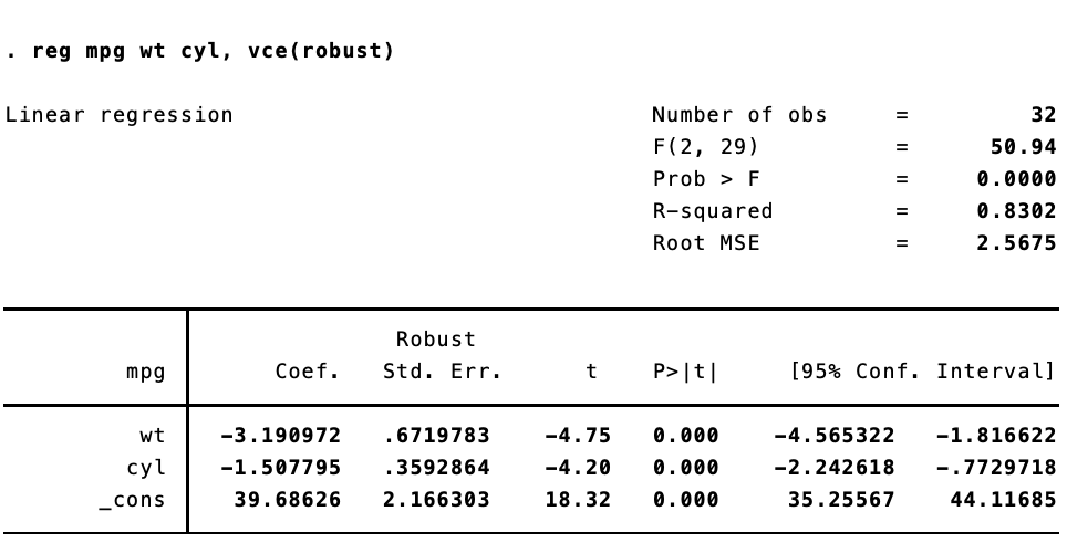
The standard errors are not quite the same. That’s because Stata implements a specific estimator. {sandwich} has a ton of options for calculating heteroskedastic- and autocorrelation-robust standard errors. To replicate the standard errors we see in Stata, we need to use type = HC1.
coeftest(fit, vcov = vcovHC(fit, type = "HC1"))
##
## t test of coefficients:
##
##             Estimate Std. Error t value  Pr(>|t|)
## (Intercept) 39.68626    2.16630 18.3198 < 2.2e-16 ***
## wt          -3.19097    0.67198 -4.7486   5.1e-05 ***
## cyl         -1.50779    0.35929 -4.1966  0.000234 ***
## ---
## Signif. codes:  0 '***' 0.001 '**' 0.01 '*' 0.05 '.' 0.1 ' ' 1
Beautiful.
Now, things get inteseting once we start to use generalized linear models. I was lead down this rabbithole by a (now deleted) post to Stack Overflow. Replicating Stata’s robust standard errors is not so simple now. Let’s say we estimate the same model, but using iteratively weight least squares estimation.
In Stata: 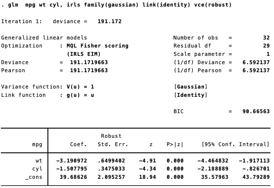
And in R:
fit <- glm(mpg ~ wt + cyl, data = mtcars, family = gaussian(link = "identity"))
coeftest(fit, vcov = vcovHC(fit, type = "HC1"))
##
## z test of coefficients:
##
##             Estimate Std. Error z value  Pr(>|z|)
## (Intercept) 39.68626    2.16630 18.3198 < 2.2e-16 ***
## wt          -3.19097    0.67198 -4.7486 2.048e-06 ***
## cyl         -1.50779    0.35929 -4.1966 2.709e-05 ***
## ---
## Signif. codes:  0 '***' 0.001 '**' 0.01 '*' 0.05 '.' 0.1 ' ' 1
They are different. Not too different, but different enough to make a difference. That’s because (as best I can figure), when calculating the robust standard errors for a glm fit, Stata is using $n / (n — 1)$ rather than $n / (n = k)$, where $n$ is the number of observations and k is the number of parameters.
I’m not getting in the weeds here, but according to this document, robust standard errors are calculated thus for linear models (see page 6):
[hat{V}(hat{beta}) = boldsymbol{D}left(frac{n}{n-k}sum_{j=1}^nhat{e}_j^2boldsymbol{x}_j^primeboldsymbol{x}_jright)boldsymbol{D}]
And for generalized linear models using maximum likelihood estimation (see page 16):
[hat{V}(hat{beta}) = boldsymbol{D}left(frac{n}{n-1}sum_{j=1}^nhat{e}_j^2boldsymbol{u}_j^primeboldsymbol{u}_jright)boldsymbol{D}]
If we make this adjustment in R, we get the same standard errors. So I have a little function to calculate Stata-like robust standard errors for glm:
robust <- function(model, stata = TRUE){

  x <- model.matrix(model)
  n <- nrow(x)
  k <- length(coef(model))

  if (stata) {
    df <- n / (n - 1)
  } else {
    df <- n / (n - k)
  }

  u <- model$residuals
  bread <- solve(crossprod(x))
  veggie_meat <- t(x) %*% (df * diag(u^2)) %*% x
  est <- bread %*% veggie_meat %*% bread

  return(est)
}
Let’s take it for a spin.
# As before
coeftest(fit, vcov = vcovHC(fit, type = "HC1"))
##
## z test of coefficients:
##
##             Estimate Std. Error z value  Pr(>|z|)
## (Intercept) 39.68626    2.16630 18.3198 < 2.2e-16 ***
## wt          -3.19097    0.67198 -4.7486 2.048e-06 ***
## cyl         -1.50779    0.35929 -4.1966 2.709e-05 ***
## ---
## Signif. codes:  0 '***' 0.001 '**' 0.01 '*' 0.05 '.' 0.1 ' ' 1
# This is the same
coeftest(fit, vcov = robust(fit, stata = FALSE))
##
## z test of coefficients:
##
##             Estimate Std. Error z value  Pr(>|z|)
## (Intercept) 39.68626    2.16630 18.3198 < 2.2e-16 ***
## wt          -3.19097    0.67198 -4.7486 2.048e-06 ***
## cyl         -1.50779    0.35929 -4.1966 2.709e-05 ***
## ---
## Signif. codes:  0 '***' 0.001 '**' 0.01 '*' 0.05 '.' 0.1 ' ' 1
# Now for the Stata-like version
coeftest(fit, vcov = robust(fit, stata = TRUE))
##
## z test of coefficients:
##
##             Estimate Std. Error z value  Pr(>|z|)
## (Intercept) 39.68626    2.09526 18.9410 < 2.2e-16 ***
## wt          -3.19097    0.64994 -4.9096 9.124e-07 ***
## cyl         -1.50779    0.34750 -4.3389 1.432e-05 ***
## ---
## Signif. codes:  0 '***' 0.001 '**' 0.01 '*' 0.05 '.' 0.1 ' ' 1
Let’s look at the Stata output again:
Success!
Of course this becomes trivial as $n$ gets larger.
Using the Ames Housing Prices data from Kaggle, we can see this. In R, estimating “non-Stata” robust standard errors:
options("scipen" = 10, "digits" = 5)

dat <- read.csv("train.csv") %>% janitor::clean_names() %>% mutate(log_price = log(sale_price))

fit <- glm(log_price ~ overall_qual + gr_liv_area, data = dat, family = gaussian(link = "identity"))
coeftest(fit, vcov = robust(fit, stata = FALSE))
##
## z test of coefficients:
##
##                Estimate Std. Error z value Pr(>|z|)
## (Intercept)  10.5486331  0.0330875  318.81   <2e-16 ***
## overall_qual  0.1788779  0.0054954   32.55   <2e-16 ***
## gr_liv_area   0.0002536  0.0000281    9.04   <2e-16 ***
## ---
## Signif. codes:  0 '***' 0.001 '**' 0.01 '*' 0.05 '.' 0.1 ' ' 1
The same model in Stata: 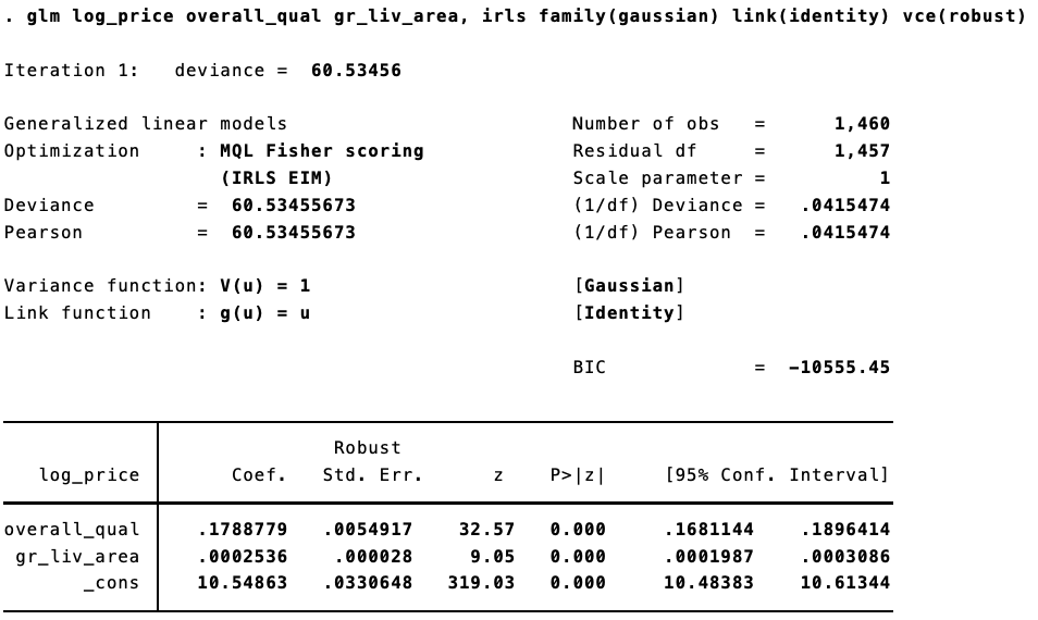
Trivial differences!