The standard error for the difference in two proportions can take different values and this depends on whether we are finding confidence interval (for the difference in proportions) or whether we are using hypothesis testing (for testing the significance of a difference in the two proportions). The following are three cases for the standard error.
Case 1: The standard error used for the confidence interval of the difference in two proportions is given by:

where  is the size of Sample 1,
  is the size of Sample 2,
  is the sample proportion of Sample 1 and
  is the sample proportion of Sample 2.
Case 2: The standard error used for hypothesis testing of difference in proportions with  is given by:
 is given by:
where  is the pooled sample proportion given by
  where
where  is the number of successes in Sample 1,
  is the number of successes in Sample 2, is the size of Sample 1 and is the size of Sample 2.
Case 3: The standard error used for hypothesis testing of difference in proportions with  is given by:
 is given by:
where is the size of Sample 1, is the size of Sample 2, is the sample proportion of Sample 1, is the sample proportion of Sample 2 and  .
.
Derivations
In the following we give a step-by-step derivation for the standard error for each case.
Suppose that we have two samples: Sample 1 of size and Sample 2 of size . Let Sample 1 consist of elements  . Each element
  (for
(for  ) could take the value 1 representing a success or the value 0 representing a fail. Let
  be the (true and unknown) population proportion for the elements found in Sample 1. That is, an element (for ) of Sample 1 has a probability
  of showing a value of 1 (i.e. of being a success). Similarly, Sample 2 is defined by the elements
  , and
, and  is the (true and unknown) population proportion for the elements found in Sample 2. Let us also define to be the number of successes in Sample 1, i.e.,
  and let be the number of successes in Sample 1, i.e.,
  .
.
We are after:
Case 1: A confidence interval for the difference in the (population) proportions, i.e.,  ,
,
Case 2: Testing the hypotheses whether or not the two (population) proportions are equal  , or,
, or,
Case 3: Testing the hypotheses whether or not the two (population) proportions differ by some particular number  .
.
However we do not known the true values of the population parameters and , and hence we rely on estimates. Let be the sample proportion of successes for Sample 1. Thus:

Let be the sample proportion of successes for Sample 1. Thus:

We are going to assume that the sampled elements are independent (that is, the fact that a sample element is 1 (or 0) has no effect on whether another element is 1 or 0). Note that each element in Sample 1 follows the Bernoulli distribution with parameter and each element in Sample 2 follows the Bernoulli distribution with parameter . Let us find the probability distributions of and . Let us first start with that for and the one for will follow in a similar fashion.
Since each is Bernoulli distributed with parameter , and assuming independence, then  follows the binomial distribution with mean
  and variance
  . Moreover, since the ‘s are i.i.d. (independently and identically distributed), then by the Central Limit Theorem, for sufficiently large , is normally distributed. Hence:

Thus:

Similarly, we can derive the probability distribution for , which is given by:

From the theory of probability, a well-known results states that the sum (or difference) of two normally-distributed random variable is normally-distributed. Thus the distribution of the difference in sample proportions  is normally distributed. The mean of is given by
  . Moreover and are independent. This follows from the fact that the sample elements are independent. Thus we have
  . The probability distribution of the difference in sample proportions is given by:

Case 1: We would like to find the confidence interval for the true difference in the two population proportions, that is,  .
.
Since: then:
 .
.
The variance of is unknown as must be estimated in order to derive the confidence interval. We use as an estimate for and as an estimate for . Thus we replace with and with in the standard deviation and obtain the following estimated standard error:
The  % confidence level for the difference in population proportions is given by:

where  is the stardardised score with a cumulative probability of
  .
.
Case 2: Here we would like to test whether there is a significant difference between the population proportion.
This is hypothesis testing using the following null and alternative hypotheses:
 :
:
 :
: 
We know that:
and thus:

Let us consider the  -statistics in the case of the null hypothesis, i.e., let us see what happens to the value of when we assume that
  . First of all we replace the in the numerator by 0. We need to replace the and the in the denominator by estimates. We are assuming that and are equal and so we just have to estimate one value. Every element in the sample, be it Sample 1 or Sample 2, has the same probability of being a success (since ). Hence
  (or pi_2) is estimated by , i.e., the number of successes in Sample 1 plus the number of successes in Sample 2, divided by the sample size. This is called the pooled sample proportion, because, since , we are combining Sample 1 with Sample 2, and thus we have just one pooled sample. So the -statistics becomes:

where .
Hence the (estimated) standard error used for hypothesis testing of a significant difference in proportions is:
Case 3: Here we would like to test whether the difference between the population proportion deviates by a certain value.
This is hypothesis testing using the following null and alternative hypotheses:
:
: 
for some pre-defined real number  .
.
We know that:
and thus:
Let us consider the -statistics in the case of the null hypothesis, i.e., let us see what happens to the value of when we assume that . First of all we replace the in the numerator by . We need to replace the and the in the denominator by estimates. We will replace by  . In Case 1, for the confidencce interval, we estimated by the sample proportion
  . However here we are going to use the information that
  . Thus we are going to estimate by a weighted average of
  and as follows:

The -statistic then becomes:

Hence the (estimated) standard error used for hypothesis testing of a difference in proportions by a certain value is:
where .
From Wikipedia, the free encyclopedia

For a value that is sampled with an unbiased normally distributed error, the above depicts the proportion of samples that would fall between 0, 1, 2, and 3 standard deviations above and below the actual value.
The standard error (SE)[1] of a statistic (usually an estimate of a parameter) is the standard deviation of its sampling distribution[2] or an estimate of that standard deviation. If the statistic is the sample mean, it is called the standard error of the mean (SEM).[1]
The sampling distribution of a mean is generated by repeated sampling from the same population and recording of the sample means obtained. This forms a distribution of different means, and this distribution has its own mean and variance. Mathematically, the variance of the sampling mean distribution obtained is equal to the variance of the population divided by the sample size. This is because as the sample size increases, sample means cluster more closely around the population mean.
Therefore, the relationship between the standard error of the mean and the standard deviation is such that, for a given sample size, the standard error of the mean equals the standard deviation divided by the square root of the sample size.[1] In other words, the standard error of the mean is a measure of the dispersion of sample means around the population mean.
In regression analysis, the term «standard error» refers either to the square root of the reduced chi-squared statistic or the standard error for a particular regression coefficient (as used in, say, confidence intervals).
Standard error of the sample mean[edit]
Exact value[edit]
Suppose a statistically independent sample of  observations
  is taken from a statistical population with a standard deviation of
  . The mean value calculated from the sample,
  , will have an associated standard error on the mean,
  , given by:[1]
 .
.

Practically this tells us that when trying to estimate the value of a population mean, due to the factor  , reducing the error on the estimate by a factor of two requires acquiring four times as many observations in the sample; reducing it by a factor of ten requires a hundred times as many observations.
Estimate[edit]
The standard deviation of the population being sampled is seldom known. Therefore, the standard error of the mean is usually estimated by replacing with the sample standard deviation  instead:
- .

As this is only an estimator for the true «standard error», it is common to see other notations here such as:
- or alternately .


A common source of confusion occurs when failing to distinguish clearly between:
Accuracy of the estimator[edit]
When the sample size is small, using the standard deviation of the sample instead of the true standard deviation of the population will tend to systematically underestimate the population standard deviation, and therefore also the standard error. With n = 2, the underestimate is about 25%, but for n = 6, the underestimate is only 5%. Gurland and Tripathi (1971) provide a correction and equation for this effect.[3] Sokal and Rohlf (1981) give an equation of the correction factor for small samples of n < 20.[4] See unbiased estimation of standard deviation for further discussion.
Derivation[edit]
The standard error on the mean may be derived from the variance of a sum of independent random variables,[5] given the definition of variance and some simple properties thereof. If are independent samples from a population with mean and standard deviation , then we can define the total

which due to the Bienaymé formula, will have variance

where we’ve approximated the standard deviations, i.e., the uncertainties, of the measurements themselves with the best value for the standard deviation of the population. The mean of these measurements is simply given by
- .

The variance of the mean is then

The standard error is, by definition, the standard deviation of which is simply the square root of the variance:
- .

For correlated random variables the sample variance needs to be computed according to the Markov chain central limit theorem.
Independent and identically distributed random variables with random sample size[edit]
There are cases when a sample is taken without knowing, in advance, how many observations will be acceptable according to some criterion. In such cases, the sample size  is a random variable whose variation adds to the variation of
  such that,
- [6]

If has a Poisson distribution, then  with estimator
  . Hence the estimator of
  becomes
  , leading the following formula for standard error:

(since the standard deviation is the square root of the variance)
Student approximation when σ value is unknown[edit]
In many practical applications, the true value of σ is unknown. As a result, we need to use a distribution that takes into account that spread of possible σ’s.
When the true underlying distribution is known to be Gaussian, although with unknown σ, then the resulting estimated distribution follows the Student t-distribution. The standard error is the standard deviation of the Student t-distribution. T-distributions are slightly different from Gaussian, and vary depending on the size of the sample. Small samples are somewhat more likely to underestimate the population standard deviation and have a mean that differs from the true population mean, and the Student t-distribution accounts for the probability of these events with somewhat heavier tails compared to a Gaussian. To estimate the standard error of a Student t-distribution it is sufficient to use the sample standard deviation «s» instead of σ, and we could use this value to calculate confidence intervals.
Note: The Student’s probability distribution is approximated well by the Gaussian distribution when the sample size is over 100. For such samples one can use the latter distribution, which is much simpler.
Assumptions and usage[edit]
An example of how  is used is to make confidence intervals of the unknown population mean. If the sampling distribution is normally distributed, the sample mean, the standard error, and the quantiles of the normal distribution can be used to calculate confidence intervals for the true population mean. The following expressions can be used to calculate the upper and lower 95% confidence limits, where is equal to the sample mean, is equal to the standard error for the sample mean, and 1.96 is the approximate value of the 97.5 percentile point of the normal distribution:
- Upper 95% limit and
- Lower 95% limit


In particular, the standard error of a sample statistic (such as sample mean) is the actual or estimated standard deviation of the sample mean in the process by which it was generated. In other words, it is the actual or estimated standard deviation of the sampling distribution of the sample statistic. The notation for standard error can be any one of SE, SEM (for standard error of measurement or mean), or SE.
Standard errors provide simple measures of uncertainty in a value and are often used because:
- in many cases, if the standard error of several individual quantities is known then the standard error of some function of the quantities can be easily calculated;
- when the probability distribution of the value is known, it can be used to calculate an exact confidence interval;
- when the probability distribution is unknown, Chebyshev’s or the Vysochanskiï–Petunin inequalities can be used to calculate a conservative confidence interval; and
- as the sample size tends to infinity the central limit theorem guarantees that the sampling distribution of the mean is asymptotically normal.
Standard error of mean versus standard deviation[edit]
In scientific and technical literature, experimental data are often summarized either using the mean and standard deviation of the sample data or the mean with the standard error. This often leads to confusion about their interchangeability. However, the mean and standard deviation are descriptive statistics, whereas the standard error of the mean is descriptive of the random sampling process. The standard deviation of the sample data is a description of the variation in measurements, while the standard error of the mean is a probabilistic statement about how the sample size will provide a better bound on estimates of the population mean, in light of the central limit theorem.[7]
Put simply, the standard error of the sample mean is an estimate of how far the sample mean is likely to be from the population mean, whereas the standard deviation of the sample is the degree to which individuals within the sample differ from the sample mean.[8] If the population standard deviation is finite, the standard error of the mean of the sample will tend to zero with increasing sample size, because the estimate of the population mean will improve, while the standard deviation of the sample will tend to approximate the population standard deviation as the sample size increases.
Extensions[edit]
Finite population correction (FPC)[edit]
The formula given above for the standard error assumes that the population is infinite. Nonetheless, it is often used for finite populations when people are interested in measuring the process that created the existing finite population (this is called an analytic study). Though the above formula is not exactly correct when the population is finite, the difference between the finite- and infinite-population versions will be small when sampling fraction is small (e.g. a small proportion of a finite population is studied). In this case people often do not correct for the finite population, essentially treating it as an «approximately infinite» population.
If one is interested in measuring an existing finite population that will not change over time, then it is necessary to adjust for the population size (called an enumerative study). When the sampling fraction (often termed f) is large (approximately at 5% or more) in an enumerative study, the estimate of the standard error must be corrected by multiplying by a »finite population correction» (a.k.a.: FPC):[9]
[10]

which, for large N:

to account for the added precision gained by sampling close to a larger percentage of the population. The effect of the FPC is that the error becomes zero when the sample size n is equal to the population size N.
This happens in survey methodology when sampling without replacement. If sampling with replacement, then FPC does not come into play.
Correction for correlation in the sample[edit]

Expected error in the mean of A for a sample of n data points with sample bias coefficient ρ. The unbiased standard error plots as the ρ = 0 diagonal line with log-log slope −½.
If values of the measured quantity A are not statistically independent but have been obtained from known locations in parameter space x, an unbiased estimate of the true standard error of the mean (actually a correction on the standard deviation part) may be obtained by multiplying the calculated standard error of the sample by the factor f:

where the sample bias coefficient ρ is the widely used Prais–Winsten estimate of the autocorrelation-coefficient (a quantity between −1 and +1) for all sample point pairs. This approximate formula is for moderate to large sample sizes; the reference gives the exact formulas for any sample size, and can be applied to heavily autocorrelated time series like Wall Street stock quotes. Moreover, this formula works for positive and negative ρ alike.[11] See also unbiased estimation of standard deviation for more discussion.
See also[edit]
- Illustration of the central limit theorem
- Margin of error
- Probable error
- Standard error of the weighted mean
- Sample mean and sample covariance
- Standard error of the median
- Variance
References[edit]
- ^ a b c d Altman, Douglas G; Bland, J Martin (2005-10-15). «Standard deviations and standard errors». BMJ: British Medical Journal. 331 (7521): 903. doi:10.1136/bmj.331.7521.903. ISSN 0959-8138. PMC 1255808. PMID 16223828.
- ^ Everitt, B. S. (2003). The Cambridge Dictionary of Statistics. CUP. ISBN 978-0-521-81099-9.
- ^ Gurland, J; Tripathi RC (1971). «A simple approximation for unbiased estimation of the standard deviation». American Statistician. 25 (4): 30–32. doi:10.2307/2682923. JSTOR 2682923.
- ^ Sokal; Rohlf (1981). Biometry: Principles and Practice of Statistics in Biological Research (2nd ed.). p. 53. ISBN 978-0-7167-1254-1.
- ^ Hutchinson, T. P. (1993). Essentials of Statistical Methods, in 41 pages. Adelaide: Rumsby. ISBN 978-0-646-12621-0.
- ^ Cornell, J R, and Benjamin, C A, Probability, Statistics, and Decisions for Civil Engineers, McGraw-Hill, NY, 1970, ISBN 0486796094, pp. 178–9.
- ^ Barde, M. (2012). «What to use to express the variability of data: Standard deviation or standard error of mean?». Perspect. Clin. Res. 3 (3): 113–116. doi:10.4103/2229-3485.100662. PMC 3487226. PMID 23125963.
- ^ Wassertheil-Smoller, Sylvia (1995). Biostatistics and Epidemiology : A Primer for Health Professionals (Second ed.). New York: Springer. pp. 40–43. ISBN 0-387-94388-9.
- ^ Isserlis, L. (1918). «On the value of a mean as calculated from a sample». Journal of the Royal Statistical Society. 81 (1): 75–81. doi:10.2307/2340569. JSTOR 2340569. (Equation 1)
- ^ Bondy, Warren; Zlot, William (1976). «The Standard Error of the Mean and the Difference Between Means for Finite Populations». The American Statistician. 30 (2): 96–97. doi:10.1080/00031305.1976.10479149. JSTOR 2683803. (Equation 2)
- ^ Bence, James R. (1995). «Analysis of Short Time Series: Correcting for Autocorrelation». Ecology. 76 (2): 628–639. doi:10.2307/1941218. JSTOR 1941218.
The standard error of a statistic is actually the standard deviation of the sampling distribution of that statistic. Standard errors reflect how much sampling fluctuation a statistic will show. The inferential statistics (deductive statistics) involved in the construction of confidence intervals and significance testing are based on standard errors. Increasing the sample size, the Standard Error decreases.
In practical applications, the true value of the standard deviation of the error is unknown. As a result, the term standard error is often used to refer to an estimate of this unknown quantity.
The size of the standard error is affected by two values.
- The Standard Deviation of the population which affects the standard error. Larger the population’s standard deviation (σ), larger is standard error i.e. $frac{sigma}{sqrt{n}}$. If the population is homogeneous (which results in small population standard deviation), the standard error will also be small.
- The standard error is affected by the number of observations in a sample. A large sample will result in a small standard error of estimate (indicates less variability in the sample means)
Application
Standard errors are used in different statistical tests such as
- to measure the distribution of the sample means
- to build confidence intervals for means, proportions, differences between means, etc., for cases when population standard deviation is known or unknown.
- to determine the sample size
- in control charts for control limits for means
- in comparisons test such as z-test, t-test, Analysis of Variance, Correlation and Regression Analysis (standard error of regression), etc.
(1) Standard Error of Means
The standard error for the mean or standard deviation of the sampling distribution of the mean measures the deviation/ variation in the sampling distribution of the sample mean, denoted by $sigma_{bar{x}}$ and calculated as the function of the standard deviation of the population and respective size of the sample i.e
$sigma_{bar{x}}=frac{sigma}{sqrt{n}}$ (used when population is finite)
If the population size is infinite then ${sigma_{bar{x}}=frac{sigma}{sqrt{n}} times sqrt{frac{N-n}{N}}}$ because $sqrt{frac{N-n}{N}}$ tends towards 1 as N tends to infinity.
When standard deviation (σ) of the population is unknown, we estimate it from the sample standard deviation. In this case standard error formula is $sigma_{bar{x}}=frac{S}{sqrt{n}}$
(2) Standard Error for Proportion
Standard error for proportion can also be calculated in same manner as we calculated standard error of mean, denoted by $sigma_p$ and calculated as $sigma_p=frac{sigma}{sqrt{n}}sqrt{frac{N-n}{N}}$.
In case of finite population $sigma_p=frac{sigma}{sqrt{n}}$
in case of infinite population $sigma=sqrt{p(1-p)}=sqrt{pq}$, where p is the probability that an element possesses the studied trait and q=1-p is the probability that it does not.
(3) Standard Error for Difference between Means
Standard error for difference between two independent quantities is the square root of the of the sum of the squared standard errors of the both quantities i.e $sigma_{bar{x}_1+bar{x}_2}=sqrt{frac{sigma_1^2}{n_1}+frac{sigma_2^2}{n_2}}$, where $sigma_1^2$ and $sigma_2^2$ are the respective variances of the two independent population to be compared and $n_1+n_2$ are the respective sizes of the two samples drawn from their respective populations.
Unknown Population Variances
If the variances of the two populations are unknown, we estimate them from the two samples i.e. $sigma_{bar{x}_1+bar{x}_2}=sqrt{frac{S_1^2}{n_1}+frac{S_2^2}{n_2}}$, where $S_1^2$ and $S_2^2$ are the respective variances of the two samples drawn from their respective population.
Equal Variances are assumed
In case when it is assumed that the variance of the two populations are equal, we can estimate the value of these variances with a pooled variance $S_p^2$ calculated as a function of $S_1^2$ and $S_2^2$ i.e
[S_p^2=frac{(n_1-1)S_1^2+(n_2-1)S_2^2}{n_1+n_2-2}]
[sigma_{bar{x}_1}+{bar{x}_2}=S_p sqrt{frac{1}{n_1}+frac{1}{n_2}}]
(4) Standard Error for Difference between Proportions
The standard error of the difference between two proportions is calculated in the same way as the standard error of the difference between means is calculated i.e.
begin{eqnarray*}
sigma_{p_1-p_2}&=&sqrt{sigma_{p_1}^2+sigma_{p_2}^2}\
&=& sqrt{frac{p_1(1-p_1)}{n_1}+frac{p_2(1-p_2)}{n_2}}
end{eqnarray*}
where $p_1$ and $p_2$ are the proportion for infinite population calculated for the two samples of sizes $n_1$ and $n_2$.

Muhammad Imdad Ullah
Currently working as Assistant Professor of Statistics in Ghazi University, Dera Ghazi Khan.
Completed my Ph.D. in Statistics from the Department of Statistics, Bahauddin Zakariya University, Multan, Pakistan.
l like Applied Statistics, Mathematics, and Statistical Computing.
Statistical and Mathematical software used is SAS, STATA, GRETL, EVIEWS, R, SPSS, VBA in MS-Excel.
Like to use type-setting LaTeX for composing Articles, thesis, etc.
After reading this article you will learn about the significance of the difference between means.
Suppose we desire to test whether 12 year – old boys and 12 year old girls of Public Schools differ in mechanical ability. As the populations of such boys and girls are too large we take a random sample of such boys and girls, administer a test and compute the means of boys and girls separately.
Suppose the mean score of such boys is 50 and that of such girls is 45. We mark a difference of 5 points between the means of boys and girls. It may be a fact that such a difference could have arisen due to sampling fluctuations.
If we draw two other samples, one from the population of 12 year old boys and other from the population of 12 year old girls we will find some difference between the means if we go on repeating it for a large number of time in drawing samples of 12 year old boys and 12 year-old girls we will find that the difference between two sets of means will vary.
Sometimes this difference will be positive, sometimes negative, and sometimes zero. The distribution of these differences will form a normal distribution around a difference of zero. The SD of this distribution is called the Standard error of difference between means.
For this following symbols are used:
SEM1 – M2 or SED or σDM
Two situations arise with respect to differences between mean:
(a) Those in which means are uncorrelated/independent, and
(b) Those in which the means are correlated.
(a) SE of the difference between two independent means:
Means are uncorrelated or independent when computed from different samples or from uncorrelated tests administered to the same sample.
In such case two situations may arise:
(i) When means are uncorrelated or independent and samples are large, and
(ii) When means are uncorrelated or independent and samples are small.
(i) SE of the difference (SED) when means are uncorrelated or independent and samples are large:
In this situation the SED can be calculated by using the formula:
![]()
in which SED = Standard error of the difference of means
SEm1 = Standard error of the mean of the first sample
SEm2 = Standard error of the mean of the second sample

Example 1:
Two groups, one made up of 114 men and the other of 175 women. The mean scores of men and women in a word building test were 19.7 and 21.0 respectively and SD’s of these two groups are 6.08 and 4.89 respectively. Test whether the observed difference of 1.3 in favour of women is significant at .05 and at .01 level.
Solution:
It is a Two-tailed Test → As direction is not clear.

To test the significance of an obtained difference between two sample means we can proceed through the following steps:
Step 1:
In first step we have to be clear whether we are to make two-tailed test or one-tailed test. Here we want to test whether the difference is significant. So it is a two-tailed test.
Step 2:
We set up a null hypothesis (H0) that there is no difference between the population means of men and women in word building. We assume the difference between the population means of two groups to be zero i.e., Ho: D = 0.
Step 3:
Then we have to decide the significance level of the test. In our example we are to test the difference at .05 and .01 level of significance.
Step 4:
In this step we have to calculate the Standard Error of the difference between means i.e. SED.
As our example is uncorrelated means and large samples we have to apply the following formula to calculate SED:

Step 5:
After computing the value of SED we have to express the difference of sample means in terms of SED. As our example is a ease of large samples we will have to calculate Z where,

Step 6:
With reference to the nature of the test in our example we are to find out the critical value for Z from Table A both at .05 and at .01 level of significance.
From Table A, Z.05 = 1.96 and Z.01 = 2.58. (This means that the value of Z to be significant at .05 level or less must be 1.96 or more).
Now 1.91 < 1.96, the marked difference is not significant at .05 level (i.e. H0 is accepted).
Interpretation:
Since the sample is large, we may assume a normal distribution of Z’s. The obtained Z just fails to reach the .05 level of significance, which for large samples is 1.96.
Consequently we would not reject the null hypothesis and we would say that the obtained difference is not significant. There may actually be some difference, but we do not have sufficient assurance of it.
A more practical conclusion would be that we have insufficient evidence of any sex difference in word-building ability, at least in the kind of population sampled.
Example 2:
Data on the performance of boys and girls are given as:

Test whether the boys or girls perform better and whether the difference of 1.0 in favour of boys is significant at .05 level. If we accept the difference to be significant what would be the Type 1 error.
Solution:


1.85 < 1.96 (Z .05 = 1.96). Hence H0 is accepted and the marked difference of 1.0 in favour of boys is not significant at .05 level.
If we accept the difference to be significant we commit Type 1 error. By reading Table A we find that ± 1.85 Z includes 93.56% of cases. Hence accepting the marked difference to be significant we are 6.44% (100 – 93.56) wrong so Type 1 error is 0644.

Example 3:
Class A was taught in an intensive coaching facility whereas Class B in a normal class teaching. At the end of a school year Class A and B averaged 48 and 43 with SD 6 and 7.40 respectively.
Test whether intensive coaching has fetched gain in mean score to Class A. Class A constitutes 60 and Class B 80 students.


... 4.42 is more than Z.01 or 2.33. So Ho is rejected. The marked difference is significant at .01 level.

Hence we conclude that intensive coaching fetched good mean scores of Class A.
(ii) The SE of the difference (SED) when means are uncorrelated or independent and samples are small:
When the N’s of two independent samples are small, the SE of the difference of two means can be calculated by using following two formulae:
When scores are given:

in which x1 = X1 – M1 (i.e. deviation of scores of the first sample from the mean of the first sample).
X2 = X2 – M2 (i.e. deviation of scores of the second sample from their mean)
When Means and SD’s of both the samples are given:

Example 4:
An Interest Test is administered to 6 boys in a Vocational Training class and to 10 boys in a Latin class. Is the mean difference between the two groups significant at .05 level?


Entering Table:
D we find that with df= 14 the critical value of t at .05 level is 2.14 and at .01 level is 2.98. The calculated value of 1.78 is less than 2.14 at .05 level of significance.
Hence H0 is accepted. We conclude that there is no significant difference between the mean scores of Interest Test of two groups of boys.
Example 5:
A personality inventory is administered in a private school to 8 boys whose conduct records are exemplar, and to 5 boys whose records are very poor.
Data are given below:
![]()
Is the difference between group means significant at the .05 level? at the 01 level?

Entering Table D we find that with df 11 the critical value of t at .05 level is 2.20 and at .01 level is 3.11. The calculated value of 2.28 is just more than 2.20 but less than 3.11.
We conclude that the difference between group means is significant at .05 level but not significant at .01 level.
Example 6:
On an arithmetic reasoning test 11 ten year-old boys and 6 ten year-old girls made the following scores:

Is the mean difference of 2.50 significant at the .05 level?
Solution:
By applying formula (43 b).

Entering Table D we find that with df 15 the critical value of t at .05 level is 2.13. The obtained value of 1.01 is less than 2.13. Hence the marked difference of 2.50 is not significant at .05 level.
(b) SE of the difference between two correlated means:
(i) The single group method:
We have already dealt with the problem of determining whether the difference between two independent means is significant.
Now we are concerned with the significance of the difference between correlated means. Correlated means are obtained from the same test administered to the same group upon two occasions.
Suppose that we have administered a test to a group of children and after two weeks we are to repeat the test. We wish to measure the effect of practice or of special training upon the second set of scores. In order to determine the significance of the difference between the means obtained in the initial and final testing.
We must use the formula:
![]()
in which σM1 and σM2 = SE’s of the initial and final test means
r12 = Coefficient of correlation between scores made on initial and final tests.
Example 7:
At the beginning of the academic year, the mean score of 81 students upon an educational achievement test in reading was 35 with an SD of 5.
At the end of the session, the mean score on an equivalent form of the same test was 38 with an SD of 4. The correlation between scores made on the initial and final testing was .53. Has the class made significant progress in reading during the year?
We may tabulate our data as follows:

(Test at .01 level of significance)
Solution:
Since we are concerned only with progress or gain, this is a one-tailed test.

By applying the formula:


Since there are 81 students, there are 81 pairs of scores and 81 differences, so that the df becomes 81 – 1 or 80. From Table D, the t for 80 df is 2.38 at the .02 level. (The table gives 2.38 for the two-tailed test which is .01 for the one-tailed test).
The obtained t of 6.12 is far greater than 2.38. Hence the difference is significant. It seems certain that the class made substantial progress in reading over the school year.
(ii) Difference method:
When groups are small, we use “difference method” for sake of easy and quick calculations.
Example 8:
Ten subjects are given 5 successive trials upon a digit-symbol test of which only the scores for trials 1 and 5 are shown. Is the mean gain from initial to final trial significant?
![]()

The column of difference is found from the difference between pairs of scores. The mean difference is found to be 4, and the SD around this mean (SDD)
![]()
Calculating SE of the mean difference:
![]()
In which SEMD = Standard error of the mean difference
SD = Standard deviation around the mean difference.

The obtained t of 5.26 > 2.82. Our t of 5.26 is much larger, than the .01 level of 2.82 and there is little doubt that the gain from Trial 1 to Trial 5 is significant.
(iii) The method of equivalent groups:
Matching by pairs:
Sometimes we may be required to compare the mean performance of two equivalent groups that are matched by pairs.
In the method of equivalent groups the matching is done initially by pairs so that each person in the first group has a match in the second group.
In such cases the number of persons in both the groups is the same i.e. n1 = n2.
Here we can compute SED by using formula:
![]()
in which SEM1 andSEM2 = Standard errors of the final scores of Group—I and Group—II respectively.
r 12 = Coefficient of correlation between final scores of group I and group II.
Example 9:
Two groups were formed on the basis of the scores obtained by students in an intelligence test. One of the groups (experimental group) was given some additional instruction for a month and the other group (controlled group) was given no such instruction.
After one month both the groups were given the same test and the data relating to the final scores are given below:


Interpretation:
Entering table of t (Table D) with df 71 the critical value of t at .05 level in case of one-tailed test is 1.67. The obtained t of 2.34 > 1.67. Hence the difference is significant at .05 level.
... The mean has increased due to additional instruction.
With df of 71the critical value of t at .01 level in case of one-tailed test is 2.38. Thus obtained t of 2.34 < 2.38. Hence the difference is not significant at .01 level.
Standard Error of the Difference between other Statistics:
(i) SE of the difference between uncorrected medians:
The significance of the difference between two medians obtained from independent samples may be found from the formula:
![]()
(ii) SE of the difference between standard deviations:

Standard error of difference between percentages or proportions
The surgical registrar who investigated appendicitis cases, referred to in Chapter 3 , wonders whether the percentages of men and women in the sample differ from the percentages of all the other men and women aged 65 and over admitted to the surgical wards during the same period. After excluding his sample of appendicitis cases, so that they are not counted twice, he makes a rough estimate of the number of patients admitted in those 10 years and finds it to be about 12-13 000. He selects a systematic random sample of 640 patients, of whom 363 (56.7%) were women and 277 (43.3%) men.
The percentage of women in the appendicitis sample was 60.8% and differs from the percentage of women in the general surgical sample by 60.8 – 56.7 = 4.1%. Is this difference of any significance? In other words, could this have arisen by chance?
There are two ways of calculating the standard error of the difference between two percentages: one is based on the null hypothesis that the two groups come from the same population; the other on the alternative hypothesis that they are different. For Normally distributed variables these two are the same if the standard deviations are assumed to be the same, but in the binomial case the standard deviations depend on the estimates of the proportions, and so if these are different so are the standard deviations. Usually both methods give almost the same result.
Confidence interval for a difference in proportions or percentages
The calculation of the standard error of a difference in proportions p1 – p2 follows the same logic as the calculation of the standard error of two means; sum the squares of the individual standard errors and then take the square root. It is based on the alternative hypothesis that there is a real difference in proportions (further discussion on this point is given in Common questions at the end of this chapter).
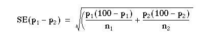
Note that this is an approximate formula; the exact one would use the population proportions rather than the sample estimates. With our appendicitis data we have:

Thus a 95% confidence interval for the difference in percentages is
4.1 – 1.96 x 4.87 to 4.1 + 1.96 x 4.87 = -5.4 to 13.6%.
Significance test for a difference in two proportions
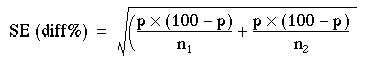
For a significance test we have to use a slightly different formula, based on the null hypothesis that both samples have a common population proportion, estimated by p.
To obtain p we must amalgamate the two samples and calculate the percentage of women in the two combined; 100 – p is then the percentage of men in the two combined. The numbers in each sample are ![]() and
and ![]() .
.
Number of women in the samples: 73 + 363 = 436
Number of people in the samples: 120 + 640 = 760
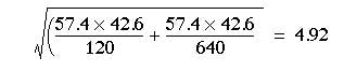
Percentage of women: (436 x 100)/760 = 57.4
Percentage of men: (324 x 100)/760 = 42.6
Putting these numbers in the formula, we find the standard error of the difference between the percentages is 4.1-1.96 x 4.87 to 4.1 + 1.96 x 4.87 = -5.4 to 13.6%
This is very close to the standard error estimated under the alternative hypothesis.
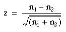
The difference between the percentage of women (and men) in the two samples was 4.1%. To find the probability attached to this difference we divide it by its standard error: z = 4.1/4.92 = 0.83. From Table A (Appendix table A.pdf) we find that P is about 0.4 and so the difference between the percentages in the two samples could have been due to chance alone, as might have been expected from the confidence interval. Note that this test gives results identical to those obtained by the ![]() test without continuity correction (described in Chapter 7).
test without continuity correction (described in Chapter 7).
Standard error of a total
The total number of deaths in a town from a particular disease varies from year to year. If the population of the town or area where they occur is fairly large, say, some thousands, and provided that the deaths are independent of one another, the standard error of the number of deaths from a specified cause is given approximately by its square root, ![]() Further, the standard error of the difference between two numbers of deaths,
Further, the standard error of the difference between two numbers of deaths, ![]()
![]() and
and ![]() , can be taken as
, can be taken as ![]() .
.
This can be used to estimate the significance of a difference between two totals by dividing the difference by its standard error:
 (6.1)
(6.1)
It is important to note that the deaths must be independently caused; for example, they must not be the result of an epidemic such as influenza. The reports of the deaths must likewise be independent; for example, the criteria for diagnosis must be consistent from year to year and not suddenly change in accordance with a new fashion or test, and the population at risk must be the same size over the period of study.
In spite of its limitations this method has its uses. For instance, in Carlisle the number of deaths from ischaemic heart disease in 1973 was 276. Is this significantly higher than the total for 1972, which was 246? The difference is 30. The standard error of the difference is ![]() . We then take z = 30/22.8 = 1.313. This is clearly much less than 1.96 times the standard error at the 5% level of probability. Reference to appendix-table.pdftable A shows that P = 0.2. The difference could therefore easily be a chance fluctuation.
. We then take z = 30/22.8 = 1.313. This is clearly much less than 1.96 times the standard error at the 5% level of probability. Reference to appendix-table.pdftable A shows that P = 0.2. The difference could therefore easily be a chance fluctuation.
This method should be regarded as giving no more than approximate but useful guidance, and is unlikely to be valid over a period of more than very few years owing to changes in diagnostic techniques. An extension of it to the study of paired alternatives follows.
Paired alternatives
Sometimes it is possible to record the results of treatment or some sort of test or investigation as one of two alternatives. For instance, two treatments or tests might be carried out on pairs obtained by matching individuals chosen by random sampling, or the pairs might consist of successive treatments of the same individual (see Chapter 7 for a comparison of pairs by the tt test). The result might then be recorded as “responded or did not respond”, “improved or did not improve”, “positive or negative”, and so on. This type of study yields results that can be set out as shown in table 6.1.
Table 6.1
| Member of pair receiving treatment A | Member of pair receiving treatment B |
|---|---|
| Responded | Responded (1) |
| Responded | Did not respond (2) |
| Did not respond | Responded (3) |
| Did not respond | Did not respond (2) |
The significance of the results can then be simply tested by McNemar’s test in the following way. Ignore rows (1) and (4), and examine rows (2) and (3). Let the larger number of pairs in either of rows (2) or (3) be called n1 and the smaller number of pairs in either of those two rows be n2. We may then use formula ( 6.1 ) to obtain the result, z. This is approximately Normally distributed under the null hypothesis, and its probability can be read from appendix-table.pdftable A.
However, in practice, the fairly small numbers that form the subject of this type of investigation make a correction advisable. We therefore diminish the difference between n1and n2 by using the following formula:
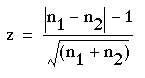
where the vertical lines mean “take the absolute value”.
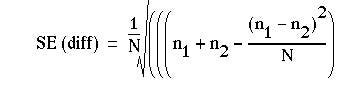
Again, the result is Normally distributed, and its probability can be read from. As for the unpaired case, there is a slightly different formula for the standard error used to calculate the confidence interval.(1) Suppose N is the total number of pairs, then
For example, a registrar in the gastroenterological unit of a large hospital in an industrial city sees a considerable number of patients with severe recurrent aphthous ulcer of the mouth. Claims have been made that a recently introduced preparation stops the pain of these ulcers and promotes quicker healing than existing preparations.
Over a period of 6 months the registrar selected every patient with this disorder and paired them off as far as possible by reference to age, sex, and frequency of ulceration. Finally she had 108 patients in 54 pairs. To one member of each pair, chosen by the toss of a coin, she gave treatment A, which she and her colleagues in the unit had hitherto regarded as the best; to the other member she gave the new treatment, B. Both forms of treatment are local applications, and they cannot be made to look alike. Consequently to avoid bias in the assessment of the results a colleague recorded the results of treatment without knowing which patient in each pair had which treatment. The results are shown in Table 6.2
| Member of pair receiving treatment A | Member of pair receiving treatment B | Pairs of patients |
|---|---|---|
| Responded | Responded | 16 |
| Responded | Did not respond | 23 |
| Did not respond | Responded | 10 |
| Did not respond | Did not respond | 5 |
| Total | 54 |
Here n1=23, n2=10. Entering these values in formula (6.1) we obtain
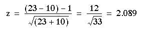
The probability value associated with 2.089 is about 0.04 Table A. Therefore we may conclude that treatment A gave significantly better results than treatment B. The standard error for the confidence interval is
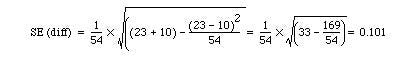
23/54 – 10/54 = 0.241
The 95% confidence interval for the difference in proportions is
0.241 – 1.96 x 0.101 to 0.241 + 1.96 x 0.10 that is, 0.043 to 0.439.
Although this does not include zero, the confidence interval is quite wide, reflecting uncertainty as to the true difference because the sample size is small. An exact method is also available.
Common questions
Why is the standard error used for calculating a confidence interval for the difference in two proportions different from the standard error used for calculating the significance?
For nominal variables the standard deviation is not independent of the mean. If we suppose that a nominal variable simply takes the value 0 or 1, then the mean is simply the proportion of is and the standard deviation is directly dependent on the mean, being largest when the mean is 0.5. The null and alternative hypotheses are hypotheses about means, either that they are the same (null) or different (alternative). Thus for nominal variables the standard deviations (and thus the standard errors) will also be different for the null and alternative hypotheses. For a confidence interval, the alternative hypothesis is assumed to be true, whereas for a significance test the null hypothesis is assumed to be true. In general the difference in the values of the two methods of calculating the standard errors is likely to be small, and use of either would lead to the same inferences. The reason this is mentioned here is that there is a close connection between the test of significance described in this chapter and the Chi square test described in Chapter 8. The difference in the arithmetic for the significance test, and that for calculating the confidence interval, could lead some readers to believe that they are unrelated, whereas in fact they are complementary. The problem does not arise with continuous variables, where the standard deviation is usually assumed independent of the mean, and is also assumed to be the same value under both the null and alternative hypotheses.
It is worth pointing out that the formula for calculating the standard error of an estimate is not necessarily unique: it depends on underlying assumptions, and so different assumptions or study designs will lead to different estimates for standard errors for data sets that might be numerically identical.
References
1. Gardner MJ, Altman DG, editors. Statistics with Confidence. London: BMJ Publishing, 1989:31.
Exercises
Exercise 6.1
In an obstetric hospital l7.8% of 320 women were delivered by forceps in 1975. What is the standard error of this percentage? In another hospital in the same region 21.2% of 185 women were delivered by forceps. What is the standard error of the difference between the percentages at this hospital and the first? What is the difference between these percentages of forceps delivery with a 95% confidence interval and what is its significance?
Exercise 6.2
A dermatologist tested a new topical application for the treatment of psoriasis on 47 patients. He applied it to the lesions on one part of the patient’s body and what he considered to be the best traditional remedy to the lesions on another but comparable part of the body, the choice of area being made by the toss of a coin. In three patients both areas of psoriasis responded; in 28 patients the disease responded to the traditional remedy but hardly or not at all to the new one; in 13 it responded to the new one but hardly or not at all to the traditional remedy; and in four cases neither remedy caused an appreciable response. Did either remedy cause a significantly better response than the other?
Errors are of various types and impact the research process in different ways. Here’s a deep exploration of the standard error, the types, implications, formula, and how to interpret the values
What is a Standard Error?
The standard error is a statistical measure that accounts for the extent to which a sample distribution represents the population of interest using standard deviation. You can also think of it as the standard deviation of your sample in relation to your target population.
The standard error allows you to compare two similar measures in your sample data and population. For example, the standard error of the mean measures how far the sample mean (average) of the data is likely to be from the true population mean—the same applies to other types of standard errors.
Explore: Survey Errors To Avoid: Types, Sources, Examples, Mitigation
Why is Standard Error Important?
First, the standard error of a sample accounts for statistical fluctuation.
Researchers depend on this statistical measure to know how much sampling fluctuation exists in their sample data. In other words, it shows the extent to which a statistical measure varies from sample to population.
In addition, standard error serves as a measure of accuracy. Using standard error, a researcher can estimate the efficiency and consistency of a sample to know precisely how a sampling distribution represents a population.
How Many Types of Standard Error Exist?
There are five types of standard error which are:
- Standard error of the mean
- Standard error of measurement
- Standard error of the proportion
- Standard error of estimate
- Residual Standard Error
1. Standard Error of the Mean (SEM)
The standard error of the mean accounts for the difference between the sample mean and the population mean. In other words, it quantifies how much variation is expected to be present in the sample mean that would be computed from every possible sample, of a given size, taken from the population.
How to Find SEM (With Formula)
SEM = Standard Deviation ÷ √n
Where;
n = sample size
Suppose that the standard deviation of observation is 15 with a sample size of 100. Using this formula, we can deduce the standard error of the mean as follows:
SEM = 15 ÷ √100
Standard Error of Mean in 1.5
2. Standard Error of Measurement
The standard error of measurement accounts for the consistency of scores within individual subjects in a test or examination.
This means it measures the extent to which estimated test or examination scores are spread around a true score.
A more formal way to look at it is through the 1985 lens of Aera, APA, and NCME. Here, they define a standard error as “the standard deviation of errors of measurement that is associated with the test scores for a specified group of test-takers….”
Read: 7 Types of Data Measurement Scales in Research
How to Find Standard Error of Measurement
Where;
rxx is the reliability of the test and is calculated as:
Rxx = S2T / S2X
Where;
S2T = variance of the true scores.
S2X = variance of the observed scores.
Suppose an organization has a reliability score of 0.4 and a standard deviation of 2.56. This means
SEm = 2.56 × √1–0.4 = 1.98
3. Standard Error of the Estimate
The standard error of the estimate measures the accuracy of predictions in sampling, research, and data collection. Specifically, it measures the distance that the observed values fall from the regression line which is the single line with the smallest overall distance from the line to the points.
How to Find Standard Error of the Estimate
The formula for standard error of the estimate is as follows:
Where;
σest is the standard error of the estimate;
Y is an actual score;
Y’ is a predicted score, and;
N is the number of pairs of scores.
The numerator is the sum of squared differences between the actual scores and the predicted scores.
4. Standard Error of Proportion
The standard of error of proportion in an observation is the difference between the sample proportion and the population proportion of your target audience. In more technical terms, this variable is the spread of the sample proportion about the population proportion.
How to Find Standard Error of the Proportion
The formula for calculating the standard error of the proportion is as follows:
Where;
P (hat) is equal to x ÷ n (with number of success x and the total number of observations of n)
5. Residual Standard Error
Residual standard error accounts for how well a linear regression model fits the observation in a systematic investigation. A linear regression model is simply a linear equation representing the relationship between two variables, and it helps you to predict similar variables.
How to Calculate Residual Standard Error
The formula for residual standard error is as follows:
Residual standard error = √Σ(y – ŷ)2/df
where:
y: The observed value
ŷ: The predicted value
df: The degrees of freedom, calculated as the total number of observations – total number of model parameters.
As you interpret your data, you should note that the smaller the residual standard error, the better a regression model fits a dataset, and vice versa.
How Do You Calculate Standard Error?
The formula for calculating standard error is as follows:
Where
σ – Standard deviation
n – Sample size, i.e., the number of observations in the sample
Here’s how this works in real-time.
Suppose the standard deviation of a sample is 1.5 with 4 as the sample size. This means:
Standard Error = 1.5 ÷ √4
That is; 1.5 ÷2 = 0.75
Alternatively, you can use a standard error calculator to speed up the process for larger data sets.
How to Interpret Standard Error Values
As stated earlier, researchers use the standard error to measure the reliability of observation. This means it allows you to compare how far a particular variable in the sample data is from the population of interest.
Calculating standard error is just one piece of the puzzle; you need to know how to interpret your data correctly and draw useful insights for your research. Generally, a small standard error is an indication that the sample mean is a more accurate reflection of the actual population mean, while a large standard error means the opposite.
Standard Error Example
Suppose you need to find the standard error of the mean of a data set using the following information:
Standard Deviation: 1.5
n = 13
Standard Error of the Mean = Standard Deviation ÷ √n
1.5 ÷ √13 = 0.42
How Should You Report the Standard Error?
After calculating the standard error of your observation, the next thing you should do is present this data as part of the numerous variables affecting your observation. Typically, researchers report the standard error alongside the mean or in a confidence interval to communicate the uncertainty around the mean.
Applications of Standard Error
The most common application of standard error are in statistics and economics. In statistics, standard error allows researchers to determine the confidence interval of their data sets, and in some cases, the margin of error. Researchers also use standard error in hypothesis testing and regression analysis.
FAQs About Standard Error
- What Is the Difference Between Standard Deviation and Standard Error of the Mean?
The major difference between standard deviation and standard error of the mean is how they account for the differences between the sample data and the population of interest.
Researchers use standard deviation to measure the variability or dispersion of a data set to its mean. On the other hand, the standard error of the mean accounts for the difference between the mean of the data sample and that of the target population.
Something else to note here is that the standard error of a sample is always smaller than the corresponding standard deviation.
- What Is The Symbol for Standard Error?
During calculation, the standard error is represented as σx̅.
- Is Standard Error the Same as Margin of Error?
No. Margin of Error and standard error are not the same. Researchers use the standard error to measure the preciseness of an estimate of a population, meanwhile margin of error accounts for the degree of error in results received from random sampling surveys.
The standard error is calculated as s / √n where;
s: Sample standard deviation
n: Sample size
On the other hand, margin of error = z*(s/√n) where:
z: Z value that corresponds to a given confidence level
s: Sample standard deviation
n: Sample size