Standard error of proportion - Исправление ошибок и поиск оптимальных решений проблем

Often in statistics we’re interested in estimating the proportion of individuals in a population with a certain characteristic.

For example, we might be interested in estimating the proportion of residents in a certain city who support a new law.

Instead of going around and asking every individual resident if they support the law, we would instead collect a simple random sample and find out how many residents in the sample support the law.

We would then calculate the sample proportion (p̂) as:

Sample Proportion Formula:

p̂ = x / n

where:

x: The count of individuals in the sample with a certain characteristic.
n: The total number of individuals in the sample.

We would then use this sample proportion to estimate the population proportion. For example, if 47 of the 300 residents in the sample supported the new law, the sample proportion would be calculated as 47 / 300 = 0.157.

This means our best estimate for the proportion of residents in the population who supported the law would be 0.157.

However, there’s no guarantee that this estimate will exactly match the true population proportion so we typically calculate the standard error of the proportion as well.

This is calculated as:

Standard Error of the Proportion Formula:

Standard Error = √p̂(1-p̂) / n

For example, if p̂ = 0.157 and n = 300, then we would calculate the standard error of the proportion as:

Standard error of the proportion = √.157(1-.157) / 300 = 0.021

We then typically use this standard error to calculate a confidence interval for the true proportion of residents who support the law.

This is calculated as:

Confidence Interval for a Population Proportion Formula:

Confidence Interval = p̂ +/- z*√p̂(1-p̂) / n

Looking at this formula, it’s easy to see that the larger the standard error of the proportion, the wider the confidence interval.

Note that the z in the formula is the z-value that corresponds to popular confidence level choices:

Confidence Level	z-value
0.90	1.645
0.95	1.96
0.99	2.58

For example, here’s how to calculate a 95% confidence interval for the true proportion of residents in the city who support the new law:

95% C.I. = p̂ +/- z*√p̂(1-p̂) / n
95% C.I. = .157 +/- 1.96*√.157(1-.157) / 300
95% C.I. = .157 +/- 1.96*(.021)
95% C.I. = [ .10884 , .19816]

Thus, we would say with 95% confidence that the true proportion of residents in the city who support the new law is between 10.884% and 19.816%.

Additional Resources

Standard Error of the Proportion Calculator
Confidence Interval for Proportion Calculator
What is a Population Proportion?

Источник

Errors are of various types and impact the research process in different ways. Here’s a deep exploration of the standard error, the types, implications, formula, and how to interpret the values

What is a Standard Error?

The standard error is a statistical measure that accounts for the extent to which a sample distribution represents the population of interest using standard deviation. You can also think of it as the standard deviation of your sample in relation to your target population.

The standard error allows you to compare two similar measures in your sample data and population. For example, the standard error of the mean measures how far the sample mean (average) of the data is likely to be from the true population mean—the same applies to other types of standard errors.

Explore: Survey Errors To Avoid: Types, Sources, Examples, Mitigation

Why is Standard Error Important?

First, the standard error of a sample accounts for statistical fluctuation.

Researchers depend on this statistical measure to know how much sampling fluctuation exists in their sample data. In other words, it shows the extent to which a statistical measure varies from sample to population.

In addition, standard error serves as a measure of accuracy. Using standard error, a researcher can estimate the efficiency and consistency of a sample to know precisely how a sampling distribution represents a population.

How Many Types of Standard Error Exist?

There are five types of standard error which are:

Standard error of the mean
Standard error of measurement
Standard error of the proportion
Standard error of estimate
Residual Standard Error

1. Standard Error of the Mean (SEM)

The standard error of the mean accounts for the difference between the sample mean and the population mean. In other words, it quantifies how much variation is expected to be present in the sample mean that would be computed from every possible sample, of a given size, taken from the population.

How to Find SEM (With Formula)

SEM = Standard Deviation ÷ √n

Where;

n = sample size

Suppose that the standard deviation of observation is 15 with a sample size of 100. Using this formula, we can deduce the standard error of the mean as follows:

SEM = 15 ÷ √100

Standard Error of Mean in 1.5

2. Standard Error of Measurement

The standard error of measurement accounts for the consistency of scores within individual subjects in a test or examination.

This means it measures the extent to which estimated test or examination scores are spread around a true score.

A more formal way to look at it is through the 1985 lens of Aera, APA, and NCME. Here, they define a standard error as “the standard deviation of errors of measurement that is associated with the test scores for a specified group of test-takers….”

Read: 7 Types of Data Measurement Scales in Research

How to Find Standard Error of Measurement

Where;

rxx is the reliability of the test and is calculated as:

Rxx = S2T / S2X

Where;

S2T = variance of the true scores.

S2X = variance of the observed scores.

Suppose an organization has a reliability score of 0.4 and a standard deviation of 2.56. This means

SEm = 2.56 × √1–0.4 = 1.98

3. Standard Error of the Estimate

The standard error of the estimate measures the accuracy of predictions in sampling, research, and data collection. Specifically, it measures the distance that the observed values fall from the regression line which is the single line with the smallest overall distance from the line to the points.

How to Find Standard Error of the Estimate

The formula for standard error of the estimate is as follows:

Where;

σest is the standard error of the estimate;

Y is an actual score;

Y’ is a predicted score, and;

N is the number of pairs of scores.

The numerator is the sum of squared differences between the actual scores and the predicted scores.

4. Standard Error of Proportion

The standard of error of proportion in an observation is the difference between the sample proportion and the population proportion of your target audience. In more technical terms, this variable is the spread of the sample proportion about the population proportion.

How to Find Standard Error of the Proportion

The formula for calculating the standard error of the proportion is as follows:

Where;

P (hat) is equal to x ÷ n (with number of success x and the total number of observations of n)

5. Residual Standard Error

Residual standard error accounts for how well a linear regression model fits the observation in a systematic investigation. A linear regression model is simply a linear equation representing the relationship between two variables, and it helps you to predict similar variables.

How to Calculate Residual Standard Error

The formula for residual standard error is as follows:

Residual standard error = √Σ(y – ŷ)2/df

where:

y: The observed value

ŷ: The predicted value

df: The degrees of freedom, calculated as the total number of observations – total number of model parameters.

As you interpret your data, you should note that the smaller the residual standard error, the better a regression model fits a dataset, and vice versa.

How Do You Calculate Standard Error?

The formula for calculating standard error is as follows:

Where

σ – Standard deviation

n – Sample size, i.e., the number of observations in the sample

Here’s how this works in real-time.

Suppose the standard deviation of a sample is 1.5 with 4 as the sample size. This means:

Standard Error = 1.5 ÷ √4

That is; 1.5 ÷2 = 0.75

Alternatively, you can use a standard error calculator to speed up the process for larger data sets.

How to Interpret Standard Error Values

As stated earlier, researchers use the standard error to measure the reliability of observation. This means it allows you to compare how far a particular variable in the sample data is from the population of interest.

Calculating standard error is just one piece of the puzzle; you need to know how to interpret your data correctly and draw useful insights for your research. Generally, a small standard error is an indication that the sample mean is a more accurate reflection of the actual population mean, while a large standard error means the opposite.

Standard Error Example

Suppose you need to find the standard error of the mean of a data set using the following information:

Standard Deviation: 1.5

n = 13

Standard Error of the Mean = Standard Deviation ÷ √n

1.5 ÷ √13 = 0.42

How Should You Report the Standard Error?

After calculating the standard error of your observation, the next thing you should do is present this data as part of the numerous variables affecting your observation. Typically, researchers report the standard error alongside the mean or in a confidence interval to communicate the uncertainty around the mean.

Applications of Standard Error

The most common application of standard error are in statistics and economics. In statistics, standard error allows researchers to determine the confidence interval of their data sets, and in some cases, the margin of error. Researchers also use standard error in hypothesis testing and regression analysis.

FAQs About Standard Error

What Is the Difference Between Standard Deviation and Standard Error of the Mean?

The major difference between standard deviation and standard error of the mean is how they account for the differences between the sample data and the population of interest.

Researchers use standard deviation to measure the variability or dispersion of a data set to its mean. On the other hand, the standard error of the mean accounts for the difference between the mean of the data sample and that of the target population.

Something else to note here is that the standard error of a sample is always smaller than the corresponding standard deviation.

What Is The Symbol for Standard Error?

During calculation, the standard error is represented as σx̅.

Is Standard Error the Same as Margin of Error?

No. Margin of Error and standard error are not the same. Researchers use the standard error to measure the preciseness of an estimate of a population, meanwhile margin of error accounts for the degree of error in results received from random sampling surveys.

The standard error is calculated as s / √n where;

s: Sample standard deviation

n: Sample size

On the other hand, margin of error = z*(s/√n) where:

z: Z value that corresponds to a given confidence level

s: Sample standard deviation

n: Sample size

Источник

From Wikipedia, the free encyclopedia

For a value that is sampled with an unbiased normally distributed error, the above depicts the proportion of samples that would fall between 0, 1, 2, and 3 standard deviations above and below the actual value.

The standard error (SE)^[1] of a statistic (usually an estimate of a parameter) is the standard deviation of its sampling distribution^[2] or an estimate of that standard deviation. If the statistic is the sample mean, it is called the standard error of the mean (SEM).^[1]

The sampling distribution of a mean is generated by repeated sampling from the same population and recording of the sample means obtained. This forms a distribution of different means, and this distribution has its own mean and variance. Mathematically, the variance of the sampling mean distribution obtained is equal to the variance of the population divided by the sample size. This is because as the sample size increases, sample means cluster more closely around the population mean.

Therefore, the relationship between the standard error of the mean and the standard deviation is such that, for a given sample size, the standard error of the mean equals the standard deviation divided by the square root of the sample size.^[1] In other words, the standard error of the mean is a measure of the dispersion of sample means around the population mean.

In regression analysis, the term «standard error» refers either to the square root of the reduced chi-squared statistic or the standard error for a particular regression coefficient (as used in, say, confidence intervals).

Standard error of the sample mean[edit]

Exact value[edit]

Suppose a statistically independent sample of observations ${displaystyle x_{1},x_{2},ldots ,x_{n}}$ is taken from a statistical population with a standard deviation of sigma . The mean value calculated from the sample, , will have an associated standard error on the mean, ${displaystyle {sigma }_{bar {x}}}$ , given by:^[1]

${displaystyle {sigma }_{bar {x}} ={frac {sigma }{sqrt {n}}}}$

Practically this tells us that when trying to estimate the value of a population mean, due to the factor , reducing the error on the estimate by a factor of two requires acquiring four times as many observations in the sample; reducing it by a factor of ten requires a hundred times as many observations.

Estimate[edit]

The standard deviation sigma of the population being sampled is seldom known. Therefore, the standard error of the mean is usually estimated by replacing sigma with the sample standard deviation $sigma _{x}$ instead:

${displaystyle {sigma }_{bar {x}} approx {frac {sigma _{x}}{sqrt {n}}}}$

As this is only an estimator for the true «standard error», it is common to see other notations here such as:

${displaystyle {widehat {sigma }}_{bar {x}}approx {frac {sigma _{x}}{sqrt {n}}}}$

or alternately ${displaystyle {s}_{bar {x}} approx {frac {s}{sqrt {n}}}}$

A common source of confusion occurs when failing to distinguish clearly between:

Accuracy of the estimator[edit]

When the sample size is small, using the standard deviation of the sample instead of the true standard deviation of the population will tend to systematically underestimate the population standard deviation, and therefore also the standard error. With n = 2, the underestimate is about 25%, but for n = 6, the underestimate is only 5%. Gurland and Tripathi (1971) provide a correction and equation for this effect.^[3] Sokal and Rohlf (1981) give an equation of the correction factor for small samples of n < 20.^[4] See unbiased estimation of standard deviation for further discussion.

Derivation[edit]

The standard error on the mean may be derived from the variance of a sum of independent random variables,^[5] given the definition of variance and some simple properties thereof. If ${displaystyle x_{1},x_{2},ldots ,x_{n}}$ are independent samples from a population with mean and standard deviation sigma , then we can define the total

${displaystyle T=(x_{1}+x_{2}+cdots +x_{n})}$

which due to the Bienaymé formula, will have variance

${displaystyle operatorname {Var} (T)approx {big (}operatorname {Var} (x_{1})+operatorname {Var} (x_{2})+cdots +operatorname {Var} (x_{n}){big )}=nsigma ^{2}.}$

where we’ve approximated the standard deviations, i.e., the uncertainties, of the measurements themselves with the best value for the standard deviation of the population. The mean of these measurements is simply given by

The variance of the mean is then

${displaystyle operatorname {Var} ({bar {x}})=operatorname {Var} left({frac {T}{n}}right)={frac {1}{n^{2}}}operatorname {Var} (T)={frac {1}{n^{2}}}nsigma ^{2}={frac {sigma ^{2}}{n}}.}$

The standard error is, by definition, the standard deviation of which is simply the square root of the variance:

${displaystyle sigma _{bar {x}}={sqrt {frac {sigma ^{2}}{n}}}={frac {sigma }{sqrt {n}}}}$

For correlated random variables the sample variance needs to be computed according to the Markov chain central limit theorem.

Independent and identically distributed random variables with random sample size[edit]

There are cases when a sample is taken without knowing, in advance, how many observations will be acceptable according to some criterion. In such cases, the sample size is a random variable whose variation adds to the variation of such that,

${displaystyle operatorname {Var} (T)=operatorname {E} (N)operatorname {Var} (X)+operatorname {Var} (N){big (}operatorname {E} (X){big )}^{2}}$

^[6]

If has a Poisson distribution, then with estimator . Hence the estimator of becomes ${displaystyle nS_{X}^{2}+n{bar {X}}^{2}}$ , leading the following formula for standard error:

${displaystyle operatorname {Standard~Error} ({bar {X}})={sqrt {frac {S_{X}^{2}+{bar {X}}^{2}}{n}}}}$

(since the standard deviation is the square root of the variance)

Student approximation when σ value is unknown[edit]

In many practical applications, the true value of σ is unknown. As a result, we need to use a distribution that takes into account that spread of possible σ’s.
When the true underlying distribution is known to be Gaussian, although with unknown σ, then the resulting estimated distribution follows the Student t-distribution. The standard error is the standard deviation of the Student t-distribution. T-distributions are slightly different from Gaussian, and vary depending on the size of the sample. Small samples are somewhat more likely to underestimate the population standard deviation and have a mean that differs from the true population mean, and the Student t-distribution accounts for the probability of these events with somewhat heavier tails compared to a Gaussian. To estimate the standard error of a Student t-distribution it is sufficient to use the sample standard deviation «s» instead of σ, and we could use this value to calculate confidence intervals.

Note: The Student’s probability distribution is approximated well by the Gaussian distribution when the sample size is over 100. For such samples one can use the latter distribution, which is much simpler.

Assumptions and usage[edit]

An example of how is used is to make confidence intervals of the unknown population mean. If the sampling distribution is normally distributed, the sample mean, the standard error, and the quantiles of the normal distribution can be used to calculate confidence intervals for the true population mean. The following expressions can be used to calculate the upper and lower 95% confidence limits, where is equal to the sample mean, is equal to the standard error for the sample mean, and 1.96 is the approximate value of the 97.5 percentile point of the normal distribution:

Upper 95% limit

{displaystyle ={bar {x}}+(operatorname {SE} times 1.96),}

and

Lower 95% limit

In particular, the standard error of a sample statistic (such as sample mean) is the actual or estimated standard deviation of the sample mean in the process by which it was generated. In other words, it is the actual or estimated standard deviation of the sampling distribution of the sample statistic. The notation for standard error can be any one of SE, SEM (for standard error of measurement or mean), or S_E.

Standard errors provide simple measures of uncertainty in a value and are often used because:

in many cases, if the standard error of several individual quantities is known then the standard error of some function of the quantities can be easily calculated;
when the probability distribution of the value is known, it can be used to calculate an exact confidence interval;
when the probability distribution is unknown, Chebyshev’s or the Vysochanskiï–Petunin inequalities can be used to calculate a conservative confidence interval; and
as the sample size tends to infinity the central limit theorem guarantees that the sampling distribution of the mean is asymptotically normal.

Standard error of mean versus standard deviation[edit]

In scientific and technical literature, experimental data are often summarized either using the mean and standard deviation of the sample data or the mean with the standard error. This often leads to confusion about their interchangeability. However, the mean and standard deviation are descriptive statistics, whereas the standard error of the mean is descriptive of the random sampling process. The standard deviation of the sample data is a description of the variation in measurements, while the standard error of the mean is a probabilistic statement about how the sample size will provide a better bound on estimates of the population mean, in light of the central limit theorem.^[7]

Put simply, the standard error of the sample mean is an estimate of how far the sample mean is likely to be from the population mean, whereas the standard deviation of the sample is the degree to which individuals within the sample differ from the sample mean.^[8] If the population standard deviation is finite, the standard error of the mean of the sample will tend to zero with increasing sample size, because the estimate of the population mean will improve, while the standard deviation of the sample will tend to approximate the population standard deviation as the sample size increases.

Extensions[edit]

Finite population correction (FPC)[edit]

The formula given above for the standard error assumes that the population is infinite. Nonetheless, it is often used for finite populations when people are interested in measuring the process that created the existing finite population (this is called an analytic study). Though the above formula is not exactly correct when the population is finite, the difference between the finite- and infinite-population versions will be small when sampling fraction is small (e.g. a small proportion of a finite population is studied). In this case people often do not correct for the finite population, essentially treating it as an «approximately infinite» population.

If one is interested in measuring an existing finite population that will not change over time, then it is necessary to adjust for the population size (called an enumerative study). When the sampling fraction (often termed f) is large (approximately at 5% or more) in an enumerative study, the estimate of the standard error must be corrected by multiplying by a »finite population correction» (a.k.a.: FPC):^[9]
^[10]

${displaystyle operatorname {FPC} ={sqrt {frac {N-n}{N-1}}}}$

which, for large N:

${displaystyle operatorname {FPC} approx {sqrt {1-{frac {n}{N}}}}={sqrt {1-f}}}$

to account for the added precision gained by sampling close to a larger percentage of the population. The effect of the FPC is that the error becomes zero when the sample size n is equal to the population size N.

This happens in survey methodology when sampling without replacement. If sampling with replacement, then FPC does not come into play.

Correction for correlation in the sample[edit]

Expected error in the mean of A for a sample of n data points with sample bias coefficient ρ. The unbiased standard error plots as the ρ = 0 diagonal line with log-log slope −½.

If values of the measured quantity A are not statistically independent but have been obtained from known locations in parameter space x, an unbiased estimate of the true standard error of the mean (actually a correction on the standard deviation part) may be obtained by multiplying the calculated standard error of the sample by the factor f:

$f={sqrt {frac {1+rho }{1-rho }}},$

where the sample bias coefficient ρ is the widely used Prais–Winsten estimate of the autocorrelation-coefficient (a quantity between −1 and +1) for all sample point pairs. This approximate formula is for moderate to large sample sizes; the reference gives the exact formulas for any sample size, and can be applied to heavily autocorrelated time series like Wall Street stock quotes. Moreover, this formula works for positive and negative ρ alike.^[11] See also unbiased estimation of standard deviation for more discussion.

References[edit]

^ ^a ^b ^c ^d Altman, Douglas G; Bland, J Martin (2005-10-15). «Standard deviations and standard errors». BMJ: British Medical Journal. 331 (7521): 903. doi:10.1136/bmj.331.7521.903. ISSN 0959-8138. PMC 1255808. PMID 16223828.
^ Everitt, B. S. (2003). The Cambridge Dictionary of Statistics. CUP. ISBN 978-0-521-81099-9.
^ Gurland, J; Tripathi RC (1971). «A simple approximation for unbiased estimation of the standard deviation». American Statistician. 25 (4): 30–32. doi:10.2307/2682923. JSTOR 2682923.
^ Sokal; Rohlf (1981). Biometry: Principles and Practice of Statistics in Biological Research (2nd ed.). p. 53. ISBN 978-0-7167-1254-1.
^ Hutchinson, T. P. (1993). Essentials of Statistical Methods, in 41 pages. Adelaide: Rumsby. ISBN 978-0-646-12621-0.
^ Cornell, J R, and Benjamin, C A, Probability, Statistics, and Decisions for Civil Engineers, McGraw-Hill, NY, 1970, ISBN 0486796094, pp. 178–9.
^ Barde, M. (2012). «What to use to express the variability of data: Standard deviation or standard error of mean?». Perspect. Clin. Res. 3 (3): 113–116. doi:10.4103/2229-3485.100662. PMC 3487226. PMID 23125963.
^ Wassertheil-Smoller, Sylvia (1995). Biostatistics and Epidemiology : A Primer for Health Professionals (Second ed.). New York: Springer. pp. 40–43. ISBN 0-387-94388-9.
^ Isserlis, L. (1918). «On the value of a mean as calculated from a sample». Journal of the Royal Statistical Society. 81 (1): 75–81. doi:10.2307/2340569. JSTOR 2340569. (Equation 1)
^ Bondy, Warren; Zlot, William (1976). «The Standard Error of the Mean and the Difference Between Means for Finite Populations». The American Statistician. 30 (2): 96–97. doi:10.1080/00031305.1976.10479149. JSTOR 2683803. (Equation 2)
^ Bence, James R. (1995). «Analysis of Short Time Series: Correcting for Autocorrelation». Ecology. 76 (2): 628–639. doi:10.2307/1941218. JSTOR 1941218.

Источник

The standard error of a statistic is actually the standard deviation of the sampling distribution of that statistic. Standard errors reflect how much sampling fluctuation a statistic will show. The inferential statistics (deductive statistics) involved in the construction of confidence intervals and significance testing are based on standard errors. Increasing the sample size, the Standard Error decreases.

In practical applications, the true value of the standard deviation of the error is unknown. As a result, the term standard error is often used to refer to an estimate of this unknown quantity.

The size of the standard error is affected by two values.

The Standard Deviation of the population which affects the standard error. Larger the population’s standard deviation (σ), larger is standard error i.e. $frac{sigma}{sqrt{n}}$. If the population is homogeneous (which results in small population standard deviation), the standard error will also be small.
The standard error is affected by the number of observations in a sample. A large sample will result in a small standard error of estimate (indicates less variability in the sample means)

Application

Standard errors are used in different statistical tests such as

to measure the distribution of the sample means
to build confidence intervals for means, proportions, differences between means, etc., for cases when population standard deviation is known or unknown.
to determine the sample size
in control charts for control limits for means
in comparisons test such as z-test, t-test, Analysis of Variance, Correlation and Regression Analysis (standard error of regression), etc.

(1) Standard Error of Means

The standard error for the mean or standard deviation of the sampling distribution of the mean measures the deviation/ variation in the sampling distribution of the sample mean, denoted by $sigma_{bar{x}}$ and calculated as the function of the standard deviation of the population and respective size of the sample i.e

$sigma_{bar{x}}=frac{sigma}{sqrt{n}}$ (used when population is finite)

If the population size is infinite then ${sigma_{bar{x}}=frac{sigma}{sqrt{n}} times sqrt{frac{N-n}{N}}}$ because $sqrt{frac{N-n}{N}}$ tends towards 1 as N tends to infinity.

When standard deviation (σ) of the population is unknown, we estimate it from the sample standard deviation. In this case standard error formula is $sigma_{bar{x}}=frac{S}{sqrt{n}}$

(2) Standard Error for Proportion

Standard error for proportion can also be calculated in same manner as we calculated standard error of mean, denoted by $sigma_p$ and calculated as $sigma_p=frac{sigma}{sqrt{n}}sqrt{frac{N-n}{N}}$.

In case of finite population $sigma_p=frac{sigma}{sqrt{n}}$
in case of infinite population $sigma=sqrt{p(1-p)}=sqrt{pq}$, where p is the probability that an element possesses the studied trait and q=1-p is the probability that it does not.

(3) Standard Error for Difference between Means

Standard error for difference between two independent quantities is the square root of the of the sum of the squared standard errors of the both quantities i.e $sigma_{bar{x}_1+bar{x}_2}=sqrt{frac{sigma_1^2}{n_1}+frac{sigma_2^2}{n_2}}$, where $sigma_1^2$ and $sigma_2^2$ are the respective variances of the two independent population to be compared and $n_1+n_2$ are the respective sizes of the two samples drawn from their respective populations.

Unknown Population Variances
If the variances of the two populations are unknown, we estimate them from the two samples i.e. $sigma_{bar{x}_1+bar{x}_2}=sqrt{frac{S_1^2}{n_1}+frac{S_2^2}{n_2}}$, where $S_1^2$ and $S_2^2$ are the respective variances of the two samples drawn from their respective population.

Equal Variances are assumed
In case when it is assumed that the variance of the two populations are equal, we can estimate the value of these variances with a pooled variance $S_p^2$ calculated as a function of $S_1^2$ and $S_2^2$ i.e

[S_p^2=frac{(n_1-1)S_1^2+(n_2-1)S_2^2}{n_1+n_2-2}]
[sigma_{bar{x}_1}+{bar{x}_2}=S_p sqrt{frac{1}{n_1}+frac{1}{n_2}}]

(4) Standard Error for Difference between Proportions

The standard error of the difference between two proportions is calculated in the same way as the standard error of the difference between means is calculated i.e.
begin{eqnarray*}
sigma_{p_1-p_2}&=&sqrt{sigma_{p_1}^2+sigma_{p_2}^2}\
&=& sqrt{frac{p_1(1-p_1)}{n_1}+frac{p_2(1-p_2)}{n_2}}
end{eqnarray*}
where $p_1$ and $p_2$ are the proportion for infinite population calculated for the two samples of sizes $n_1$ and $n_2$.

Muhammad Imdad Ullah

Currently working as Assistant Professor of Statistics in Ghazi University, Dera Ghazi Khan.
Completed my Ph.D. in Statistics from the Department of Statistics, Bahauddin Zakariya University, Multan, Pakistan.
l like Applied Statistics, Mathematics, and Statistical Computing.
Statistical and Mathematical software used is SAS, STATA, GRETL, EVIEWS, R, SPSS, VBA in MS-Excel.
Like to use type-setting LaTeX for composing Articles, thesis, etc.

Источник

Home
Statistics
Standard Error Calculator

getcalc.com’s Standard Error (SE) of mean or proportion calculator to estimate the standard deviation of mean x̄ or proportion p of sampling distribution, difference between two sample means or proportions (using either standard deviation or p value) in statistical surveys & experiments. This calculator featured to generate the step by step work for any corresponding input values to help grade school students to solve standard error worksheet problems online by using standard deviation or without using standard deviation (using p value).

Standard Error of Statistic & its Applications

In probability & statistics, the standard deviation of sampling distribution of a statistic is called as Standard Error often abbreviated as SE. It shows how effective the selected sample size n is in the statistical experiments or the reliability of experiment results with respect to the sample size. In other words, it’s a numerical value that represents standard deviation of the sampling distribution of a statistic for sample mean x̄ or proportion p, difference between two sample means (x̄₁ — x̄₂) or proportions (p₁ — p₂) (using either standard deviation or p value) in statistical surveys & experiments. It is one of an important & most frequently used functions in statistics & probability. Setup the test of significance or hypothesis for large & small sample size (student’s t & Z statistic) to measure the reliability of sample & population parameter and the estimation the confidence interval for population parameter are some of the major applications of standard error. It’s a statistic measure calculated from the sampling distributions where the large size samples or proportions reduces the SE of a statistic proportionally and vice versa. For quick calculations & reference, users may use this SE calculator to estimate or generate the complete work with steps for SE of sample mean (x̄), SE of sample proportion (p), difference between two sample means (x̄₁ — x̄₂) & difference between two sample proportions (p₁ — p₂).

Standard Error (SE) & Formulas

Work with Steps for Standard Error Calculation

Источник

The standard error for the difference in two proportions can take different values and this depends on whether we are finding confidence interval (for the difference in proportions) or whether we are using hypothesis testing (for testing the significance of a difference in the two proportions). The following are three cases for the standard error.

Case 1: The standard error used for the confidence interval of the difference in two proportions is given by:

$S.E.=sqrt{frac{p_1(1-p_1)}{n_1}+frac{p_2(1-p_2)}{n_2}}$

where is the size of Sample 1, is the size of Sample 2, is the sample proportion of Sample 1 and is the sample proportion of Sample 2.

Case 2: The standard error used for hypothesis testing of difference in proportions with is given by:

$S.E.=sqrt{P(1-P)(frac{1}{n_1}+frac{1}{n_2})}$

where is the pooled sample proportion given by $P=frac{r_1+r_2}{n_1+n_2}$ where is the number of successes in Sample 1, is the number of successes in Sample 2, is the size of Sample 1 and is the size of Sample 2.

Case 3: The standard error used for hypothesis testing of difference in proportions with is given by:

$S.E.=sqrt{frac{p_1(1-p_1)}{n_1}+frac{p'_2(1-p'_2)}{n_2}}$

where is the size of Sample 1, is the size of Sample 2, is the sample proportion of Sample 1, is the sample proportion of Sample 2 and $p'_2=frac{n_1(c-p_1)+n_2p_2}{n_1+n_2}$ .

Derivations

In the following we give a step-by-step derivation for the standard error for each case.

Suppose that we have two samples: Sample 1 of size and Sample 2 of size . Let Sample 1 consist of elements $X_{11},X_{12},cdots,X_{1n_1}$ . Each element $X_{1i}$ (for ) could take the value 1 representing a success or the value 0 representing a fail. Let be the (true and unknown) population proportion for the elements found in Sample 1. That is, an element $X_{1i}$ (for ) of Sample 1 has a probability of showing a value of 1 (i.e. of being a success). Similarly, Sample 2 is defined by the elements $X_{21}, X_{22}, cdots, X_{2n_2}$ , and is the (true and unknown) population proportion for the elements found in Sample 2. Let us also define to be the number of successes in Sample 1, i.e., $r_1=X_{11}+X_{12}+cdots+X_{1n_1}$ and let be the number of successes in Sample 1, i.e., $r_2=X_{21}+X_{22}+cdots+X_{2n_2}$ .

We are after:

Case 1: A confidence interval for the difference in the (population) proportions, i.e., ,

Case 2: Testing the hypotheses whether or not the two (population) proportions are equal , or,

Case 3: Testing the hypotheses whether or not the two (population) proportions differ by some particular number .

However we do not known the true values of the population parameters and , and hence we rely on estimates. Let be the sample proportion of successes for Sample 1. Thus:

$p_1=frac{X_{11}+X_{12}+cdots+X_{1n_1}}{n_1}=frac{r_1}{n_1}$

Let be the sample proportion of successes for Sample 1. Thus:

$p_2=frac{X_{21}+X_{22}+cdots+X_{2n_2}}{n_2}=frac{r_2}{n_2}$

We are going to assume that the sampled elements are independent (that is, the fact that a sample element is 1 (or 0) has no effect on whether another element is 1 or 0). Note that each element in Sample 1 follows the Bernoulli distribution with parameter and each element in Sample 2 follows the Bernoulli distribution with parameter . Let us find the probability distributions of and . Let us first start with that for and the one for will follow in a similar fashion.

Since each $X_{1i}$ is Bernoulli distributed with parameter , and assuming independence, then $r_1=frac{X_{11}+X_{12}+cdots+X_{1n_1}}{n_1}$ follows the binomial distribution with mean and variance . Moreover, since the $X_{1i}$ ‘s are i.i.d. (independently and identically distributed), then by the Central Limit Theorem, for sufficiently large , is normally distributed. Hence:

$r_1sim mathcall{N}(n_1pi_1,n_1pi_1(1-pi_1))$

Thus:

$p_1=frac{r_1}{n_1}sim mathcall{N}(pi_1,frac{pi_1(1-pi_1)}{n_1})$

Similarly, we can derive the probability distribution for , which is given by:

$p_2sim mathcall{N}(pi_2,frac{pi_2(1-pi_2)}{n_2})$

From the theory of probability, a well-known results states that the sum (or difference) of two normally-distributed random variable is normally-distributed. Thus the distribution of the difference in sample proportions is normally distributed. The mean of is given by $mathbb{E}(p_1-p_2)=mathbb{E}(p_1)-mathbb{E}(p_2)=pi_1-pi_2$ . Moreover and are independent. This follows from the fact that the sample elements are independent. Thus we have $Var(p_1-p_1)=Var(p_1)+Var(p_2)=frac{pi_1(1-pi_1)}{n_1}+frac{pi_2(1-pi_2)}{n_2}$ . The probability distribution of the difference in sample proportions is given by:

$p_1-p_2sim mathcall{N}(pi_1-pi_2,frac{pi_1(1-pi_1)}{n_1}+frac{pi_2(1-pi_2)}{n_2})$

Case 1: We would like to find the confidence interval for the true difference in the two population proportions, that is, .

Since: $p_1-p_2sim mathcall{N}(pi_1-pi_2,frac{pi_1(1-pi_1)}{n_1}+frac{pi_2(1-pi_2)}{n_2})$ then:

$Z=frac{p_1-p_2-(pi_1-pi_2)}{sqrt{frac{pi_1(1-pi_1)}{n_1}+frac{pi_2(1-pi_2)}{n_2}}}sim mathcal{N}(0,1)$ .

The variance of is unknown as must be estimated in order to derive the confidence interval. We use as an estimate for and as an estimate for . Thus we replace with and with in the standard deviation and obtain the following estimated standard error:

$S.E.=sqrt{frac{p_1(1-p_1)}{n_1}+frac{p_2(1-p_2)}{n_2}}$

The % confidence level for the difference in population proportions is given by:

$p_1-p_2-z_frac{alpha}{2} S.E.leq pi_1-pi_2 leq p_1-p_2+z_frac{alpha}{2} S.E.$

where $z_frac{alpha}{2}$ is the stardardised score with a cumulative probability of $1-frac{alpha}{2}$ .

Case 2: Here we would like to test whether there is a significant difference between the population proportion.

This is hypothesis testing using the following null and alternative hypotheses:

We know that:

$p_1-p_2sim mathcall{N}(pi_1-pi_2,frac{pi_1(1-pi_1)}{n_1}+frac{pi_2(1-pi_2)}{n_2})$

and thus:

$Z=frac{p_1-p_2-(pi_1-pi_2)}{sqrt{frac{pi_1(1-pi_1)}{n_1}+frac{pi_2(1-pi_2)}{n_2}}}$

Let us consider the -statistics in the case of the null hypothesis, i.e., let us see what happens to the value of when we assume that . First of all we replace the in the numerator by 0. We need to replace the and the in the denominator by estimates. We are assuming that and are equal and so we just have to estimate one value. Every element in the sample, be it Sample 1 or Sample 2, has the same probability of being a success (since ). Hence (or pi_2) is estimated by $P=frac{r_1+r_2}{n_1+n_2}$ , i.e., the number of successes in Sample 1 plus the number of successes in Sample 2, divided by the sample size. This is called the pooled sample proportion, because, since , we are combining Sample 1 with Sample 2, and thus we have just one pooled sample. So the -statistics becomes:

$begin{equation*} begin{split} Z&=frac{p_1-p_2-0}{sqrt{frac{P(1-P)}{n_1}+frac{P(1-P)}{n_2}}}\ &=frac{p_1-p_2}{sqrt{P(1-P)(frac{1}{n_1}+frac{1}{n_2})}} end{split} end{equation*}$

where $P=frac{r_1+r_2}{n_1+n_2}$ .

Hence the (estimated) standard error used for hypothesis testing of a significant difference in proportions is:

$S.E.=sqrt{P(1-P)(frac{1}{n_1}+frac{1}{n_2})}$

Case 3: Here we would like to test whether the difference between the population proportion deviates by a certain value.

This is hypothesis testing using the following null and alternative hypotheses:

for some pre-defined real number .

We know that:

$p_1-p_2sim mathcall{N}(pi_1-pi_2,frac{pi_1(1-pi_1)}{n_1}+frac{pi_2(1-pi_2)}{n_2})$

and thus:

$Z=frac{p_1-p_2-(pi_1-pi_2)}{sqrt{frac{pi_1(1-pi_1)}{n_1}+frac{pi_2(1-pi_2)}{n_2}}}$

Let us consider the -statistics in the case of the null hypothesis, i.e., let us see what happens to the value of when we assume that . First of all we replace the in the numerator by . We need to replace the and the in the denominator by estimates. We will replace by $p_1=frac{r_1}{n_1}$ . In Case 1, for the confidencce interval, we estimated by the sample proportion $p_2=frac{r_2}{n_2}$ . However here we are going to use the information that . Thus we are going to estimate by a weighted average of and as follows:

$begin{equation*} begin{split} p'_2&=frac{n_1}{n_1+n_2}(c-p_1)+frac{n_2}{n_1+n_2}p_2\ &=frac{n_1(c-p_1)+n_2p_2}{n_1+n_2} end{split} end{equation*}$

The -statistic then becomes:

$Z=frac{p_1-p_2-c}{sqrt{frac{p_1(1-p_1)}{n_1}+frac{p'_2(1-p'_2)}{n_2}}}$

Hence the (estimated) standard error used for hypothesis testing of a difference in proportions by a certain value is:

$S.E.=sqrt{frac{p_1(1-p_1)}{n_1}+frac{p'_2(1-p'_2)}{n_2}}$

where $p'_2=frac{n_1(c-p_1)+n_2p_2}{n_1+n_2}$ .

Источник

This tutorial will explain how to calculate standard error for a sample proportion, for cases when the population standard deviation is known, and when it is unknown. Our discussion breaks down as follows:

Standard Error for Sample Proportions (Population Standard Deviation Is Unknown)
Standard Error for Sample Proportions (Population Standard Deviation Is Known)

1. Standard Error for Sample Proportions (Population Standard Deviation Is Unknown)

A survey is conducted at the local high schools to find out about underage drinking. Of the 523 students who replied to the survey, 188 replied that they have drank some amount of alcohol.

What is the standard error of the sample proportion?

These students are either answering yes or no on the survey: «Yes, I’ve drank some amount of alcohol» or «No, I have not drank some amount of alcohol». That is qualitative data, also known as categorical data. Therefore, we’re dealing with a sample proportion.

Whenever we’re dealing with a sample proportion, the next question we need to ask ourselves is, «Do I know the population standard deviation?» In this case, we do not have any of that information. Therefore, the formula to calculate the standard error is p-hat times q-hat, divided by n, all under the square root.

Standard Error for Sample Proportions (Population Standard Deviation Unknown)

$table attributes columnalign left end attributes row cell square root of fraction numerator p with hat on top space q with hat on top over denominator n end fraction end root end cell row cell p with hat on top equals s a m p l e space p r o p o r t i o n space o f space s u c c e s s end cell row cell q with hat on top equals c o m p l e m e n t space o f space p with hat on top end cell row cell n equals s a m p l e space s i z e end cell end table$

We’re actually going to use the data that was given to us, which are estimates—that’s what the hat indicates—in order to calculate the standard error.

The first thing we need to do is to figure out what p-hat is, based off of the information given to us. In this case, the p-hat is what we’re interested in, and that is how many have answered yes to participating in underage drinking. That would be 188 out of 523 students, or 188/523, which is about 36% of the students.

Now, we also need the complement, which would be q-hat. This is also written as 1 minus p-hat. One minus the 188 out of 523, or 1 — 0.36, tells us that 0.64, or 64%, of the students have not participated in underage drinking. To always make sure our math is correct, remember that our p-hat and q-hat should add up to 1, because they’re complements of each other.

Now, we can plug in those values into the formula.

$square root of fraction numerator p with hat on top space q with hat on top over denominator n end fraction end root equals square root of fraction numerator left parenthesis 0.36 right parenthesis left parenthesis 0.64 right parenthesis over denominator 523 end fraction end root equals square root of fraction numerator 0.2304 over denominator 523 end fraction end root equals square root of 0.00044 end root equals 0.021$

We have 0.36 for p-hat, 0.64 for q-hat, and the total sample, n, was 523 students. This calculates to a standard error that is 0.021.

2. Standard Error for Sample Proportions (Population Standard Deviation Is Known)

Revisiting our prior example, a survey is conducted at the local high schools to find out about underage drinking. Of the 523 students who replied to the survey, 188 replied that they have drank some amount of alcohol. The proportion of underage drinkers nationally is 39%

What is the standard error of the sample proportion?

We are still looking at the students who were surveyed about underage drinking, but notice how this scenario added on that the proportion of underage drinkers nationally is 39%. We’re still calculating the standard error of the sample proportion, but in this case, we know the population standard deviation, which is 39%. We’re going to use the formula of the square root of pq over n.

Standard Error for Sample Proportions (Population Standard Deviation Is Known)

$table attributes columnalign left end attributes row cell square root of fraction numerator p q over denominator n end fraction end root end cell row cell p equals p o p u l a t i o n space p r o p o r t i o n space o f space s u c c e s s end cell row cell q equals c o m p l e m e n t space o f space p end cell row cell n equals s a m p l e space s i z e end cell end table$

We do not need to use p-hat, which is the 188 out of 523, to make the estimate for the standard error. We actually know p, which is 39%, or 0.39.

In this case, we’re going to use 0.39 for p. This is another way of indicating population proportion. We can then use this to find q, which is the complement of p. The complement of 0.39 is calculated by 1 minus 0.39, which equals 0.61, or 61%. Sometimes we’ll see this written as p subscript 0 and q subscript 0.

The sample size, n, is still 523 students who were surveyed.

$square root of fraction numerator p q over denominator n end fraction end root equals square root of fraction numerator left parenthesis 0.39 right parenthesis left parenthesis 0.61 right parenthesis over denominator 523 end fraction end root equals square root of fraction numerator 0.2379 over denominator 523 end fraction end root equals square root of 0.000455 end root equals 0.021$

The standard error is 0.021.

Today we learned how to calculate standard error of a sample proportion, and practiced identifying which formula to use, based on the whether the population standard deviation is unknown or known.

Источник

The UK Faculty of Public Health has recently taken ownership of the Health Knowledge resource. This new, advert-free website is still under development and there may be some issues accessing content. Additionally, the content has not been audited or verified by the Faculty of Public Health as part of an ongoing quality assurance process and as such certain material included maybe out of date. If you have any concerns regarding content you should seek to independently verify this.

Introduction

Learning objectives: You will learn about standard error of a mean, standard error of a proportion, reference ranges, and confidence intervals. The earlier sections covered estimation of statistics. This section considers how precise these estimates may be. Please now read the resource text below.

Resource text

Standard error of the mean

A series of samples drawn from one population will not be identical. They will show chance variations from one to another, and the variation may be slight or considerable. For example, a series of samples of the body temperature of healthy people would show very little variation from one to another, but the variation between samples of the systolic blood pressure would be considerable. Thus the variation between samples depends partly on the amount of variation in the population from which they are drawn. Furthermore, it is a matter of common observation that a small sample is a much less certain guide to the population from which it was drawn than a large sample. In other words, the more people that are included in a sample, the greater chance that the sample will accurately represent the population, provided that a random process is used to construct the sample. A consequence of this is that if two or more samples are drawn from a population, then the larger they are, the more likely they are to resemble each other — again, provided that the random sampling technique is followed. Thus the variation between samples depends partly also on the size of the sample. If we draw a series of samples and calculate the mean of the observations in each, we have a series of means.

These means generally follow a normal distribution, and they often do so even if the observations from which they were obtained do not. This can be proven mathematically and is known as the «Central Limit Theorem». The series of means, like the series of observations in each sample, has a standard deviation. The standard error of the mean of one sample is an estimate of the standard deviation that would be obtained from the means of a large number of samples drawn from that population.

As noted above, if random samples are drawn from a population, their means will vary from one to another. The variation depends on the variation of the population and the size of the sample. We do not know the variation in the population so we use the variation in the sample as an estimate of it. This is expressed in the standard deviation. If we now divide the standard deviation by the square root of the number of observations in the sample we have an estimate of the standard error of the mean. It is important to realise that we do not have to take repeated samples in order to estimate the standard error; there is sufficient information within a single sample. However, the concept is that if we were to take repeated random samples from the population, this is how we would expect the mean to vary, purely by chance.

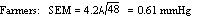
Example 1 A general practitioner has been investigating whether the diastolic blood pressure of men aged 20-44 differs between printers and farm workers. For this purpose, she has obtained a random sample of 72 printers and 48 farm workers and calculated the mean and standard deviations, as shown in table 1. Table 1: Mean diastolic blood pressures of printers and farmers

	Number	Mean diastolic blood pressure (mmHg)	Standard deviation (mmHg)
Printers	72	88	4.5
Farmers	48	79	4.2

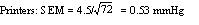
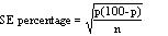
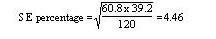
To calculate the standard errors of the two mean blood pressures, the standard deviation of each sample is divided by the square root of the number of the observations in the sample. These standard errors may be used to study the significance of the difference between the two means. Standard error of a proportion or a percentage Just as we can calculate a standard error associated with a mean so we can also calculate a standard error associated with a percentage or a proportion. Here the size of the sample will affect the size of the standard error but the amount of variation is determined by the value of the percentage or proportion in the population itself, and so we do not need an estimate of the standard deviation. Example 2 A senior surgical registrar in a large hospital is investigating acute appendicitis in people aged 65 and over. As a preliminary study he examines the hospital case notes over the previous 10 years and finds that of 120 patients in this age group with a diagnosis confirmed at operation, 73 (60.8%) were women and 47 (39.2%) were men. If p represents one percentage, 100-p represents the other. Then the standard error of each of these percentages is obtained by (1) multiplying them together, (2) dividing the product by the number in the sample, and (3) taking the square root:

which for the appendicitis data given above is as follows:

Reference ranges

Swinscow and Campbell (2002) describe 140 children who had a mean urinary lead concentration of 2.18 mmol /24h, with standard deviation 0.87. The points that include 95% of the observations are 2.18 (1.96 x 0.87), giving an interval of 0.48 to 3.89. One of the children had a urinary lead concentration of just over 4.0 mmol /24h. This observation is greater than 3.89 and so falls in the 5% of observations beyond the 95% probability limits. We can say that the probability of each of these observations occurring is 5%. Another way of looking at this is to see that if you chose one child at random out of the 140, the chance that the child’s urinary lead concentration will exceed 3.89, or is less than 0.48, is 5%. This probability is usually used expressed as a fraction of 1 rather than of 100, and written as p<0.05. Standard deviations thus set limits about which probability statements can be made. Some of these are set out in table 2. Table 2: Probabilities of multiples of standard deviation for a normal distribution

Number of standard deviations (z)	Probability of getting an observation at least as far from the mean (two sided P)
0	1.00
0.5	0.62
1.0	0.31
1.5	0.13
2.0	0.045
2.5	0.012
3.0	0.0027

To estimate the probability of finding an observed value, say a urinary lead concentration of 4.8 mmol /24h, in sampling from the same population of observations as the 140 children provided, we proceed as follows. The distance of the new observation from the mean is 4.8 — 2.18 = 2.62. How many standard deviations does this represent? Dividing the difference by the standard deviation gives 2.62/0.87 = 3.01. Table 2 shows that the probability is very close to 0.0027. This probability is small, so the observation probably did not come from the same population as the 140 other children. To take another example, the mean diastolic blood pressure of printers was found to be 88 mmHg and the standard deviation 4.5 mmHg. One of the printers had a diastolic blood pressure of 100 mmHg. The mean plus or minus 1.96 times its standard deviation gives the following two figures:

We can say therefore that only 1 in 20 (or 5%) of printers in the population from which the sample is drawn would be expected to have a diastolic blood pressure below 79 or above about 97 mmHg. These are the 95% limits. The 99.73% limits lie three standard deviations below and three above the mean. The blood pressure of 100 mmHg noted in one printer thus lies beyond the 95% limit of 97 but within the 99.73% limit of 101.5 (= 88 + (3 x 4.5)). The 95% limits are often referred to as a «reference range». For many biological variables, they define what is regarded as the normal (meaning standard or typical) range. Anything outside the range is regarded as abnormal. Given a sample of disease free subjects, an alternative method of defining a normal range would be simply to define points that exclude 2.5% of subjects at the top end and 2.5% of subjects at the lower end. This would give an empirical normal range . Thus in the 140 children we might choose to exclude the three highest and three lowest values. However, it is much more efficient to use the mean +/- 2SD, unless the dataset is quite large (say >400).

Confidence intervals

The means and their standard errors can be treated in a similar fashion. If a series of samples are drawn and the mean of each calculated, 95% of the means would be expected to fall within the range of two standard errors above and two below the mean of these means. This common mean would be expected to lie very close to the mean of the population. So the standard error of a mean provides a statement of probability about the difference between the mean of the population and the mean of the sample. In our sample of 72 printers, the standard error of the mean was 0.53 mmHg. The sample mean plus or minus 1.96 times its standard error gives the following two figures:

This is called the 95% confidence interval , and we can say that there is only a 5% chance that the range 86.96 to 89.04 mmHg excludes the mean of the population. If we take the mean plus or minus three times its standard error, the interval would be 86.41 to 89.59. This is the 99.73% confidence interval, and the chance of this interval excluding the population mean is 1 in 370. Confidence intervals provide the key to a useful device for arguing from a sample back to the population from which it came. With small samples — say under 30 observations — larger multiples of the standard error are needed to set confidence limits. These come from a distribution known as the t distribution, for which the reader is referred to Swinscow and Campbell (2002). Confidence interval for a proportion In a survey of 120 people operated on for appendicitis 37 were men. The standard error for the percentage of male patients with appendicitis is given by:

In this case this is 0.0446 or 4.46%. This is also the standard error of the percentage of female patients with appendicitis, since the formula remains the same if p is replaced by 100-p. With this standard error we can get 95% confidence intervals on the two percentages:

These confidence intervals exclude 50%. We can conclude that males are more likely to get appendicitis than females. This formula is only approximate, and works best if n is large and p between 0.1 and 0.9. A better method would be to use a chi-squared test, which is to be discussed in a later module. There is much confusion over the interpretation of the probability attached to confidence intervals. To understand it, we have to resort to the concept of repeated sampling. Imagine taking repeated samples of the same size from the same population. For each sample, calculate a 95% confidence interval. Since the samples are different, so are the confidence intervals. We know that 95% of these intervals will include the population parameter. However, without any additional information we cannot say which ones. Thus with only one sample, and no other information about the population parameter, we can say there is a 95% chance of including the parameter in our interval. Note that this does not mean that we would expect, with 95% probability, that the mean from another sample is in this interval.

Video 1: A video summarising confidence intervals. (This video footage is taken from an external site. The content is optional and not necessary to answer the questions.)

References

Altman DG, Bland JM. BMJ 2005, Statistics Note Standard deviations and standard errors. Swinscow TDV, and Campbell MJ. BMJ Books 2009, Statistics at Square One, 10 th ed. Chapter 4.

Additional Resources

What is a Standard Error?

Why is Standard Error Important?

How Many Types of Standard Error Exist?

1. Standard Error of the Mean (SEM)

2. Standard Error of Measurement

3. Standard Error of the Estimate

4. Standard Error of Proportion

5. Residual Standard Error

How Do You Calculate Standard Error?

How to Interpret Standard Error Values

Standard Error Example

How Should You Report the Standard Error?

Applications of Standard Error

FAQs About Standard Error

Standard error of the sample mean[edit]

Exact value[edit]

Estimate[edit]

Accuracy of the estimator[edit]

Derivation[edit]

Independent and identically distributed random variables with random sample size[edit]

Student approximation when σ value is unknown[edit]

Assumptions and usage[edit]

Standard error of mean versus standard deviation[edit]

Extensions[edit]

Finite population correction (FPC)[edit]

Correction for correlation in the sample[edit]

See also[edit]

References[edit]

Application

(1) Standard Error of Means

(2) Standard Error for Proportion

(3) Standard Error for Difference between Means

(4) Standard Error for Difference between Proportions

Standard Error of Statistic & its Applications

Standard Error (SE) & Formulas

Work with Steps for Standard Error Calculation

Case 1: The standard error used for the confidence interval of the difference in two proportions is given by:

Derivations

Case 2: Here we would like to test whether there is a significant difference between the population proportion.

Case 3: Here we would like to test whether the difference between the population proportion deviates by a certain value.

1. Standard Error for Sample Proportions (Population Standard Deviation Is Unknown)

2. Standard Error for Sample Proportions (Population Standard Deviation Is Known)

Introduction

Resource text

Standard error of the mean

Reference ranges

Confidence intervals

References

Related links