Standard error of regression python - Исправление ошибок и поиск оптимальных решений проблем

A residual is the difference between an observed value and a predicted value in a regression model.

It is calculated as:

Residual = Observed value – Predicted value

If we plot the observed values and overlay the fitted regression line, the residuals for each observation would be the vertical distance between the observation and the regression line:

One type of residual we often use to identify outliers in a regression model is known as a standardized residual.

It is calculated as:

r_i = e_i / s(e_i) = e_i / RSE√1-h_ii

where:

e_i: The i^th residual
RSE: The residual standard error of the model
h_ii: The leverage of the i^th observation

In practice, we often consider any standardized residual with an absolute value greater than 3 to be an outlier.

This tutorial provides a step-by-step example of how to calculate standardized residuals in Python.

Step 1: Enter the Data

First, we’ll create a small dataset to work with in Python:

import pandas as pd

#create dataset
df = pd.DataFrame({'x': [8, 12, 12, 13, 14, 16, 17, 22, 24, 26, 29, 30],
                   'y': [41, 42, 39, 37, 35, 39, 45, 46, 39, 49, 55, 57]})

Step 2: Fit the Regression Model

Next, we’ll fit a simple linear regression model:

import statsmodels.api as sm

#define response variable
y = df['y']

#define explanatory variable
x = df['x']

#add constant to predictor variables
x = sm.add_constant(x)

#fit linear regression model
model = sm.OLS(y, x).fit()

Step 3: Calculate the Standardized Residuals

Next, we’ll calculate the standardized residuals of the model:

#create instance of influence
influence = model.get_influence()

#obtain standardized residuals
standardized_residuals = influence.resid_studentized_internal

#display standardized residuals
print(standardized_residuals)

[ 1.40517322  0.81017562  0.07491009 -0.59323342 -1.2482053  -0.64248883
  0.59610905 -0.05876884 -2.11711982 -0.066556    0.91057211  1.26973888]

From the results we can see that none of the standardized residuals exceed an absolute value of 3. Thus, none of the observations appear to be outliers.

Step 4: Visualize the Standardized Residuals

Lastly, we can create a scatterplot to visualize the values for the predictor variable vs. the standardized residuals:

import matplotlib.pyplot as plt

plt.scatter(df.x, standardized_residuals)
plt.xlabel('x')
plt.ylabel('Standardized Residuals')
plt.axhline(y=0, color='black', linestyle='--', linewidth=1)
plt.show()

Additional Resources

What Are Residuals?
What Are Standardized Residuals?
How to Calculate Standardized Residuals in R
How to Calculate Standardized Residuals in Excel

Источник

This article is to tell you the whole interpretation of the regression summary table. There are many statistical softwares that are used for regression analysis like Matlab, Minitab, spss, R etc. but this article uses python. The Interpretation is the same for other tools as well. This article needs the basics of statistics including basic knowledge of regression, degrees of freedom, standard deviation, Residual Sum Of Squares(RSS), ESS, t statistics etc.

In regression there are two types of variables i.e. dependent variable (also called explained variable) and independent variable (explanatory variable).

The regression line used here is,

$hat{Y}_{i}=-3.2002+0.7529 X_{i}$

The summary table of the regression is given below.

                                    OLS Regression Results                            
        ==============================================================================
        Dep. Variable:                      y   R-squared:                       0.669
        Model:                            OLS   Adj. R-squared:                  0.667
        Method:                 Least Squares   F-statistic:                     299.2
        Date:                Mon, 01 Mar 2021   Prob (F-statistic):           2.33e-37
        Time:                        16:19:34   Log-Likelihood:                -88.686
        No. Observations:                 150   AIC:                             181.4
        Df Residuals:                     148   BIC:                             187.4
        Df Model:                           1                                         
        Covariance Type:            nonrobust                                         
        ==============================================================================
                         coef    std err          t      P>|t|      [0.025      0.975]
        ------------------------------------------------------------------------------
        const         -3.2002      0.257    -12.458      0.000      -3.708      -2.693
        x1             0.7529      0.044     17.296      0.000       0.667       0.839
        ==============================================================================
        Omnibus:                        3.538   Durbin-Watson:                   1.279
        Prob(Omnibus):                  0.171   Jarque-Bera (JB):                3.589
        Skew:                           0.357   Prob(JB):                        0.166
        Kurtosis:                       2.744   Cond. No.                         43.4
        ==============================================================================

Dependent variable: Dependent variable is one that is going to depend on other variables. In this regression analysis Y is our dependent variable because we want to analyse the effect of X on Y.

Model: The method of Ordinary Least Squares(OLS) is most widely used model due to its efficiency. This model gives best approximate of true population regression line. The principle of OLS is to minimize the square of errors ( ∑e_i² ).

Number of observations: The number of observation is the size of our sample, i.e. N = 150.

Degree of freedom(df) of residuals:

Degree of freedom is the number of independent observations on the basis of which the sum of squares is calculated.

D.f Residuals = 150 – (1+1) = 148

Degree of freedom(D.f) is calculated as,

Degrees of freedom, D . f = N – K

Where, N = sample size(no. of observations) and K = number of variables + 1

Df of model:

Df of model = K – 1 = 2 – 1 = 1 ,

Where, K = number of variables + 1

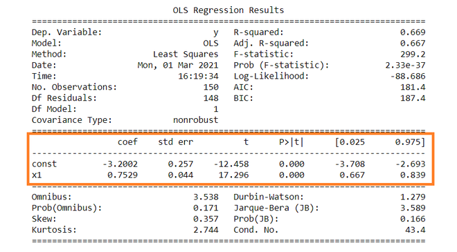
Constant term: The constant terms is the intercept of the regression line. From regression line (eq…1) the intercept is -3.002. In regression we omits some independent variables that do not have much impact on the dependent variable, the intercept tells the average value of these omitted variables and noise present in model.

Coefficient term: The coefficient term tells the change in Y for a unit change in X i.e if X rises by 1 unit then Y rises by 0.7529. If you are familiar with derivatives then you can relate it as the rate of change of Y with respect to X .

Standard error of parameters: Standard error is also called the standard deviation. Standard error shows the sampling variability of these parameters. Standard error is calculated by as –

Standard error of intercept term (b1):

$s eleft(b_{1}right)=sqrt{left(frac{sum x_{i}^{2}}{n sumleft(x_{i}-bar{x}right)^{2}}right) sigma^{2}}$

Standard error of coefficient term(b2):

$s eleft(b_{2}right)=sqrt{frac{sigma^{2}}{sumleft(x_{i}-bar{x}right)}}$

Here, σ²is the Standard error of regression (SER) . And σ² is equal to RSS( Residual Sum Of Square i.e ∑e_i² ).

t – statistics:

In theory, we assume that error term follows the normal distribution and because of this the parameters b₁and b₂ also have normal distributions with variance calculated in above section.

That is ,

b₁ ∼ N(B₁, σ_b1²)
b₂∼ N(B_{2 ,}σ_b2²)

Here B₁and B₂ are true means of b1 and b2.

t – statistics are calculated by assuming following hypothesis –

H₀ : B₂ = 0 ( variable X has no influence on Y)
H_a : B₂ ≠ 0 (X has significant impact on Y)

Calculations for t – statistics :

t = ( b₁– B₁) / s.e (b₁)

From summary table , b₁= -3.2002 and se(b₁) = 0.257, So,

t = (-3.2002 – 0) / 0.257 = -12.458

Similarly, b₂= 0.7529 , se(b₂) = 0.044

t = (0.7529 – 0) / 0.044 = 17.296

p – values:

In theory, we read that p-value is the probability of obtaining the t statistics at least as contradictory to H₀ as calculated from assuming that the null hypothesis is true. In the summary table, we can see that P-value for both parameters is equal to 0. This is not exactly 0, but since we have very larger statistics (-12.458 and 17.296) p-value will be approximately 0.

If you know about significance levels then you can see that we can reject the null hypothesis at almost every significance level.

Confidence intervals:

There are many approaches to test the hypothesis, including the p-value approach mentioned above. The confidence interval approach is one of them. 5% is the standard significance level (∝) at which C.I’s are made.

C.I for B₁is ( b₁– t_∝/2 s.e(b₁) , b₁+ t_∝/2 s.e(b₁) )

Since ∝ = 5 %, b₁= -3.2002, s.e(b₁)=0.257 , from t table , t_0.025,148= 1.655,

After putting values the C.I for B₁is approx. ( -3.708 , -2.693 ). Same can be done for b₂as well.

While calculating p values we rejected the null hypothesis we can see same in C.I as well. Since 0 does not lie in any of the intervals so we will reject the null hypothesis.

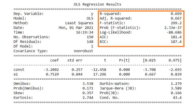
R – squared value:

R²is the coefficient of determination that tells us that how much percentage variation independent variable can be explained by independent variable. Here, 66.9 % variation in Y can be explained by X. The maximum possible value of R²can be 1, means the larger the R² value better the regression.

F – statistic:

F test tells the goodness of fit of a regression. The test is similar to the t-test or other tests we do for the hypothesis. The F – statistic is calculated as below –

$F=frac{R^{2} /(k-1)}{left(1-R^{2}right) /(n-k)}$

Inserting the values of R², n and k, F = (0.669/1) / (0.331/148) = 229.12.

You can calculate the probability of F >229.1 for 1 and 148 df, which comes to approx. 0. From this, we again reject the null hypothesis stated above.

The remaining terms are not often used. Terms like Skewness and Kurtosis tells about the distribution of data. Skewness and kurtosis for the normal distribution are 0 and 3 respectively. Jarque-Bera test is used for checking whether an error has normal distribution or not.

Источник

Linear Regression using Python

In the previous article, we studied Data Science. One thing that I believe is that if we can correlate anything with us or our life, there are greater chances of understanding the concept. So I will try to explain everything by relating it to humans.

What is Regression and Why is it called so?

Regression is an ML algorithm that can be trained to predict real numbered outputs; like temperature, stock price, etc. Regression is based on a hypothesis that can be linear, quadratic, polynomial, non-linear, etc. The hypothesis is a function based on some hidden parameters and input values. In the training phase, the hidden parameters are optimized w.r.t. the input values presented in the training. The process that does the optimization is the gradient descent algorithm. You also need a Back-propagation algorithm that can be used to compute the gradient at each layer, If you are using neural networks. Once the hypothesis parameters got trained (when they gave the least error during the training), then the same hypothesis with the trained parameters is used with new input values to predict outcomes that will be again real values.

Advantages/Features of Linear Regression

Linear regression is an extremely simple method.
It is very easy and intuitive to use and understand.
A person with only the knowledge of high school mathematics can understand and use it.
In addition, it works in most cases. Even when it doesn’t fit the data exactly, we can use it to find the nature of the relationship between the two variables.

Disadvantages/Shortcomings of Linear Regression

By its definition, linear regression only models relationships between dependent and independent variables that are linear. It assumes there is a straight-line relationship between them which is incorrect sometimes. Linear regression is very sensitive to the anomalies in the data (or outliers).
Take for example most of your data lies in the range 0-10. If due to any reason only one of the data items comes out of the range, say for example 15, this significantly influences the regression coefficients.
Another disadvantage is that if we have a number of parameters than the number of samples available then the model starts to model the noise rather than the relationship between the variables.

Types of Regression

1. Linear regression is used for predictive analysis. Linear regression is a linear approach for modeling the relationship between the criterion or the scalar response and the multiple predictors or explanatory variables. Linear regression focuses on the conditional probability distribution of the response given the values of the predictors. For linear regression, there is a danger of overfitting. The formula for linear regression is Y’ = bX + A.

2. Logistic regression is used when the dependent variable is dichotomous. Logistic regression estimates the parameters of a logistic model and is a form of binomial regression. Logistic regression is used to deal with data that has two possible criteria and the relationship between the criteria and the predictors. The equation for logistic regression is l = $beta_{0}+beta_{1}x_{1}+beta_{2}x_{2}$ .

3. Polynomial regression is used for curvilinear data. Polynomial regression is fit with the method of least squares. The goal of regression analysis to model the expected value of a dependent variable y in regards to the independent variable x. The equation for polynomial regression is l = $beta_{0}+beta_{0}x_{1}+epsilon$

4. Stepwise regression is used for fitting regression models with predictive models. It is carried out automatically. With each step, the variable is added or subtracted from the set of explanatory variables. The approaches for stepwise regression are forward selection, backward elimination, and bidirectional elimination. The formula for stepwise regression is $b_{j.std} = b_{j}(s_{x} * s_{y}^{-1})$

5. Ridge regression is a technique for analyzing multiple regression data. When multicollinearity occurs, least squares estimates are unbiased. A degree of bias is added to the regression estimates, and a result, ridge regression reduces the standard errors. The formula for ridge regression is $beta = (X^{T}X + lambda * I)^{-1}X^{T}y$

6. Lasso regression is a regression analysis method that performs both variable selection and regularization. Lasso regression uses soft thresholding. Lasso regression selects only a subset of the provided covariates for use in the final model. Lasso regression is: $N^{-1}sum^{N}_{i=1}f(x_{i}, y_{I}, alpha, beta)$ .

7. ElasticNet regression is a regularized regression method that linearly combines the penalties of the lasso and ridge methods. ElasticNet regression is used to support vector machines, metric learning, and portfolio optimization. The penalty function is given by: $|| beta ||_1=sum^{p}_{j=1}|beta_j|$

8. Support Vector regression is a regression method where we identify a hyperplane with maximum margin such that the maximum number of data points are within that margin. SVRs are almost similar to the SVM classification algorithm. Instead of minimizing the error rate as in simple linear regression, we try to fit the error within a certain threshold. Our objective in SVR is to basically consider the points that are within the margin. Our best fit line is the hyperplane that has the maximum number of points.

9. Decision Tree regression is a regression where the ID3 algorithm can be used to identify the splitting node by reducing the standard deviation (in classification information gain is used).
A decision tree is built by partitioning the data into subsets containing instances with similar values (homogenous). Standard deviation is used to calculate the homogeneity of a numerical sample. If the numerical sample is completely homogeneous, its standard deviation is zero.

10. Random Forest regression is an ensemble approach where we take into account the predictions of several decision regression trees.

Select K random points
Identify n where n is the number of decision tree regressors to be created. Repeat steps 1 and 2 to create several regression trees.
The average of each branch is assigned to the leaf node in each decision tree.
To predict output for a variable, the average of all the predictions of all decision trees are taken into consideration.

Random Forest prevents overfitting (which is common in decision trees) by creating random subsets of the features and building smaller trees using these subsets.

Key Terms

1. Estimator

A formula or algorithm for generating estimates of parameters, given relevant data.

2. Bias

An estimate is unbiased if its expectation equals the value of the parameter being estimated; otherwise, it is biased.

3.Efficiency

An estimator A is more efficient than an estimator B if A has a smaller sampling variance — that is, if the particular values generated by A are more tightly clustered around their expectation.

4. Consistency

An estimator is consistent if the estimates it produces converge on the true parameter value as the sample size increases without limit. Consider an estimator that produces estimates θ^ of some parameter θ, and let ^ denote a small number. If the estimator is consistent, we can make the probability as close to 1.0 as we like or as small as we like by drawing a sufficiently large sample. Note that a biased estimator may nonetheless be consistent if the bias tends to zero in the limit. Conversely, an unbiased estimator may be inconsistent if its sampling variance fails to shrink appropriately as the sample size increases.

5. Standard error of the Regression (SER)

An estimate of the standard deviation of the error term in a regression model.

6. R-squared

A standardized measure of the goodness of fit for a regression model.

7. Standard error of regression coefficient

An estimate of the standard deviation of the sampling distribution for the coefficient in question.

8. P-value

The probability, supposing the null hypothesis to be true, of drawing sample data that are as adverse to the null as the data are actually drawn, or more so. When a small p-value is found, the two possibilities are that we happened to draw a low-probability unrepresentative sample or that the null hypothesis is in fact false.

9. Significance level

For a hypothesis test, this is the smallest p-value for which we will not reject the null hypothesis. If we choose a significance level of 1%, we’re saying that we’ll reject the null if and only if the p-value for the test is less than 0.01. The significance level is also the probability of making a type 1 error (that is, rejecting a true null hypothesis).

10. T-test

The t-test (or z-test, which is the same thing asymptotically) is a common test for the null hypothesis that a particular regression parameter, βi, has some specific value (commonly zero, but generically βH0).

11. F-test

A common procedure for jointly testing a set of linear restrictions on a regression model.

12. Multicollinearity

A situation where there is a high degree of correlation among the independent variables in a regression model — or, more generally, where some of the Xs are close to being linear combinations of other Xs. Symptoms include large standard errors and the inability to produce precise parameter estimates. This is not a serious problem if one is primarily interested in forecasting; it is a problem is one is trying to estimate causal influences.

13. Omitted variable bias

Bias in the estimation of regression parameters that arises when a relevant independent variable is omitted from a model and the omitted variable is correlated with one or more of the included variables.

14. Log variables

A common transformation permits the estimation of a nonlinear model using OLS to substitute the natural log of a variable for the level of that variable. This can be done for the dependent variable and/or one or more independent variables. A key point to remember about logs is that for small changes, the change in the log of a variable is a good approximation to the proportional change in the variable itself. For example, if log(y) changes by 0.04, y changes by about 4%.

15. Quadratic terms

Another common transformation. When both xi and x^2_i are included as regressors, it is important to remember that the estimated effect of xi on y is given by the derivative of the regression equation with respect to xi. If the coefficient on xi is β and the coefficient on x 2 i is γ, the derivative is β + 2γ xi.

16. Interaction terms

Pairwise products of the «original» independent variables. The inclusion of interaction terms in a regression allows for the possibility that the degree to which xi affects y depends on the value of some other variable x j. In other words, x j modulates the effect of xi on y. For example, the effect of experience on wages (xi) might depend on the gender (x j) of the worker.

17. Independent Variable

An independent variable is a variable that is changed or controlled in a scientific experiment to test the effects on the dependent variable.

18. Dependent Variable

A dependent variable is a variable being tested and measured in a scientific experiment. The dependent variable is ‘dependent’ on the independent variable. As the experimenter changes the independent variable, the effect on the dependent variable is observed and recorded.

19. Regularization

There are extensions of the training of the linear model called regularization methods. These seek to both minimize the sum of the squared error of the model on the training data (using ordinary least squares) but also to reduce the complexity of the model (like the number or absolute size of the sum of all coefficients in the model).

Gradient Descent

Gradient descent is an optimization algorithm used to minimize some function by iteratively moving in the direction of steepest descent as defined by the negative of the gradient. In machine learning, we use gradient descent to update the parameters of our model. Parameters refer to coefficients in Linear Regression and weights in neural networks.

1. Learning Rate

The size of these steps is called the learning rate. With a high learning rate, we can cover more ground each step, but we risk overshooting the lowest point since the slope of the hill is constantly changing. With a very low learning rate, we can confidently move in the direction of the negative gradient since we are recalculating it so frequently. A low learning rate is more precise, but calculating the gradient is time-consuming, so it will take us a very long time to get to the bottom.

2. Cost Function

A Loss Function or Cost Function tells us “how good” our model is at making predictions for a given set of parameters. The cost function has its own curve and its own gradients. The slope of this curve tells us how to update our parameters to make the model more accurate.

Python Implementation of Gradient Descent

def update_weights(m, b, X, Y, learning_rate):
m_deriv = 0
b_deriv = 0
N = len(X)
for i in range(N):
m_deriv += —2*X[i] * (Y[i] — (m*X[i] + b))
b_deriv += —2*(Y[i] — (m*X[i] + b))
m -= (m_deriv / float(N)) * learning_rate
b -= (b_deriv / float(N)) * learning_rate
return m, b

Remembering Variables With DRYMIX

When results are plotted in graphs, the convention is to use the independent variable as the x-axis and the dependent variable as the y-axis. The DRY MIX acronym can help keep the variables straight:

D is the dependent variable
R is the responding variable
Y is the axis on which the dependent or responding variable is graphed (the vertical axis)
M is the manipulated variable or the one that is changed in an experiment
I is the independent variable
X is the axis on which the independent or manipulated variable is graphed (the horizontal axis)

Simple Linear Regression Model

The simple linear regression model is represented like this: y = (β0 +β1 + Ε)

By mathematical convention, the two factors that are involved in simple linear regression analysis are designated x and y. The equation that describes how y is related to x is known as the regression model. The linear regression model also contains an error term that is represented by Ε, or the Greek letter epsilon. The error term is used to account for the variability in y that cannot be explained by the linear relationship between x and y. There also parameters that represent the population being studied. These parameters of the model are represented by (β0+β1x).

The simple linear regression equation is graphed as a straight line.

The simple linear regression equation is represented like this: Ε(y) = (β0 +β1*x)

β0 is the y-intercept of the regression line.
β1 is the slope.
Ε(y) is the mean or expected value of y for a given value of x.

A regression line can show a positive linear relationship, a negative linear relationship, or no relationship.

If the graphed line in a simple linear regression is flat (not sloped), there is no relationship between the two variables.
If the regression line slopes upward with the lower end of the line at the y-intercept (axis) of the graph, and the upper end of the line extending upward into the graph field, away from the x-intercept (axis) a positive linear relationship exists.
If the regression line slopes downward with the upper end of the line at the y-intercept (axis) of the graph, and the lower end of the line extending downward into the graph field, toward the x-intercept (axis) a negative linear relationship exists.

ŷ = β0 +β1*x

Important Note

1. Regression analysis is not used to interpret cause-and-effect relationships( a mechanism where one event makes another event happen, i.e each event is dependent on one-another) between variables. Regression analysis can, however, indicate how variables are related or to what extent variables are associated with each other.

2. It is also known as bivariate regression or regression analysis

Sum of Square Errors

This is the sum of differences between the points and the regression line. It can serve as a measure of how well the line fits the data.

Standard Estimate of Errors

The mean error is equal to zero. If se(sigma_epsilon) is small the errors tend to be close to zero (close to the mean error). Then, the model fits the data well. Therefore, we can use se as a measure of the suitability of using a linear model. An estimator of se is given by se(sigma_epsilon)

Coefficient of Determination

To measure the strength of the linear relationship we use the coefficient of determination. R^2 takes on any value between zero and one.

R^2 = 1: Perfect match between the line and the data points.
R^2 = 0: There is no linear relationship between x and y.

Image result for coefficient of determination formula

Simple Linear Regression Example

Let’s take the example of Housing Price Prediction, the data that I am using is KC House Prices, you can download it from the article. Feel free to use any dataset, there some very good datasets available on kaggle and with Google Colab.

Output

dataset

From the above data, we can see that we have a lot of tables, but simple linear regression can only process two columns, so we select the «price» and «sqrt_living». Here we will take the first 100 rows for our demonstration.

Before fitting the data let’s analyze the data:

import seaborn as sns
df = pd.read_csv(«kc_house_data.csv»)
sns.distplot(df[‘price’][1:100])

Output

import seaborn as sns
df = pd.read_csv(«kc_house_data.csv»)
sns.distplot(df[‘sqrt_living’][1:100])

Output

1. Demo using Numpy

In the below code, we will just use numpy to perform linear regression.

import pandas as pd
import numpy as np
import matplotlib.pyplot as plt
%matplotlib inline
def estimate_coef(x, y):
n = np.size(x)
m_x, m_y = np.mean(x), np.mean(y)
SS_xy = np.sum(y*x) — n*m_y*m_x
SS_xx = np.sum(x*x) — n*m_x*m_x
b_1 = SS_xy / SS_xx
b_0 = m_y — b_1*m_x
return(b_0, b_1)
def plot_regression_line(x, y, b):
plt.scatter(x, y, color = «m»,
marker = «o», s = 30)
y_pred = b[0] + b[1]*x
plt.plot(x, y_pred, color = «g»)
plt.xlabel(‘x’)
plt.ylabel(‘y’)
plt.show()
def main():
df = pd.read_csv(«kc_house_data.csv»)
y= df[‘price’][1:100]
x= df[‘sqft_living’][1:100]
plt.scatter(x, y)
plt.xlabel(‘x’)
plt.ylabel(‘y’)
plt.show()
b = estimate_coef(x, y)
print(«Estimated coefficients:nb_0 = {} nb_1 = {}».format(b[0], b[1]))
plot_regression_line(x, y, b)
if __name__ == «__main__»:
main()

Output

The input data can be visualized as:

After, executing the code we get the following output

Estimated coefficients: b_0 = 41517.979725295736 b_1 = 229.10249314945074

So the Linear Regression equation becomes :

[price] = 41517.979725795736+ 229.10249374945074*[sqrt_living]

i.e y = b[0] + b[1]*x

Let’s see the final plot with the Regression Line

To predict the values we run the following command:

print(«For x =100», «the predicted value would be»,(b[1]*100+b[0]))

So the predicted value that we get is 64428.22904024081

Since the machine has to learn, hence would be doing some errors in predicting, so the let’s see what percentage of error it is performing at each given point

y_diff = y -(b[1]+b[0]*x)
sns.distplot(y_diff)

2. Demo using Sklearn

In the below code, we will learn how to code linear regression using SkLearn

import pandas as pd
import numpy as np
import matplotlib.pyplot as plt
import seaborn as sns
df = pd.read_csv(«kc_house_data.csv»)
y= df[‘price’][1:100]
x= df[‘sqft_living’][1:100]
from sklearn.model_selection import train_test_split
x_train, x_test, y_train, y_test = train_test_split(x, y, test_size=0.2, random_state=101)
from sklearn.linear_model import LinearRegression
lr = LinearRegression()
x_train = x_train.values.reshape(-1,1)
lr.fit(x_train, y_train)
print(«b[0] = «,lr.intercept_)
print(«b[1] = «,lr.coef_)
x_test = x_test.values.reshape(-1,1)
pred = lr.predict(x_test)
plt.scatter(x_train,y_train)
y_pred = lr.intercept_ + lr.coef_*x_train
plt.plot(x_train, y_pred, color = «g»)
plt.xlabel(‘x’)
plt.ylabel(‘y’)
plt.show()

Output

After, executing the code we get the following output

b[0] = 21803.55365770642 b[1] = [232.07541739]

So the Linear Regression equation becomes :

[price] = 21803.55365770642+ 232.07541739*[sqrt_living]

i.e y = b[0] + b[1]*x

Let’s now see a graphical representation between the predicted value wrt test set

lr_test

Since the machine has to learn, hence would be doing some errors in predicting, so the let’s see what percentage of error it is performing at each given point

sns.distplot((y_test-pred))

3. Demo using TensorFlow

In this, I will not be using «kc_house_data.csv». To make it as simple as possible, I used some dummy data and then I will explain each and everything

np.random.seed(101)
tf.set_random_seed(101)

We first set the seed value for both NumPy and TensorFlow. The seed value is used for random number generation.

x = np.linspace(0, 50, 50)
y = np.linspace(0, 50, 50)

We now generate dummy data using the NumPy’s linspace function, which generated 50 equally distributed points between 0 and 50

x += np.random.uniform(-4, 4, 50)
y += np.random.uniform(-4, 4, 50)

Since the data so generated is too perfect, so we add a liitle bit of uniformaly distributed white noise.

n = len(x)
plt.scatter(x, y)
plt.xlabel(‘x’)
plt.xlabel(‘y’)
plt.title(«Training Data»)
plt.show()

Here, we thus plot the graphical representation of the dummy data.

X = tf.placeholder(«float»)
Y = tf.placeholder(«float»)
W = tf.Variable(np.random.randn(), name = «W»)
b = tf.Variable(np.random.randn(), name = «b»)

Here we are setting X and Y as the actual training data and the W and b as the trainable data, where:

W means Weight
b means bais
X means the dependent variable
Y means the independent variable

We have to give initial weights and bias to the model. So, we initialize them with some random values.

learning_rate = 0.01
training_epochs = 1000

Here, we assume the learning rate to be 0.01 i.e. the gradient descent value would increase/decrease by 0.01 and we will train the model 1000 times or for 1000 epochs

y_pred = tf.add(tf.multiply(X, W), b)
cost = tf.reduce_sum(tf.pow(y_pred-Y, 2)) / (2 * n)
optimizer = tf.train.GradientDescentOptimizer(learning_rate).minimize(cost)
init = tf.global_variables_initializer()

Next thing, we have to set the hypothesis, cost function, the optimizer (which will make sure that the model is learning on every epoch), and the global variable initializer.

Since we are using simple linear regression hence the hypothesis is set as:

Depedent_Variable*Weight+Bias or Depedent_Variable*b[1]+b[0]

We choose the cost function to be mean squared error cost function
We choose the optimizer as Gradient Descent with the motive of minimizing the cost with a given learning rate
We use TensorFlow’s global variable initialize the global variable so that we can re-use the value of variables

with tf.Session() as sess:
sess.run(init)
for epoch in range(training_epochs):
for (_x, _y) in zip(x, y):
sess.run(optimizer, feed_dict = {X : _x, Y : _y})
if (epoch + 1) % 50 == 0:
c = sess.run(cost, feed_dict = {X : x, Y : y})
print(«Epoch», (epoch + 1), «: cost =», c, «W =», sess.run(W), «b =», sess.run(b))

tf.Session()
we start the TensorFlow session and name the Session as sess. We then initialize all the required variable using the
sess.run(init)
initialize all the required variable using the
for epoch in range(training_epochs)
create a for loop that runs till epoch becomes equal to training_epocs
for (_x, _y) in zip (x,y)
this is used to form a set of values from the given data and then parse through the so formed sets
sess.run(optimizer, feed_dict = {X: _x, Y: _y})
used to run the first optimizer iteration on each the data points
if(epoch+1)%50==0
to break the given iterations into a batch of 50 each
c= sess.run(cost, feed_dict= {X: x, Y: y})
performs the training on the given data points
print(«Epoch»,(epoch+1),»: cost», c, «W =», sess.run(W), «b =», sess.run(b)
print the values after each 50 epochs

training_cost = sess.run(cost, feed_dict ={X: x, Y: y})
weight = sess.run(W)
bias = sess.run(b)

the above code is used to store the values for the next session

predictions = weight * x + bias
print(«Training cost =», training_cost, «Weight =», weight, «bias =», bias, ‘n’)
plt.plot(x, y, ‘ro’, label =‘Original data’)
plt.plot(x, predictions, label =‘Fitted line’)
plt.title(‘Linear Regression Result’)
plt.legend()
plt.show()

The above code demonstrates how we can use the trained model to predict values

LR_TensorFlow.py

import numpy as np
import tensorflow as tf
import matplotlib.pyplot as plt
np.random.seed(101)
tf.set_random_seed(101)
x = np.linspace(0, 50, 50)
y = np.linspace(0, 50, 50)
x += np.random.uniform(-4, 4, 50)
y += np.random.uniform(-4, 4, 50)
n = len(x)
plt.scatter(x, y)
plt.xlabel(‘x’)
plt.xlabel(‘y’)
plt.title(«Training Data»)
plt.show()
X = tf.placeholder(«float»)
Y = tf.placeholder(«float»)
W = tf.Variable(np.random.randn(), name = «W»)
b = tf.Variable(np.random.randn(), name = «b»)
learning_rate = 0.01
training_epochs = 1000
y_pred = tf.add(tf.multiply(X, W), b)
cost = tf.reduce_sum(tf.pow(y_pred-Y, 2)) / (2 * n)
optimizer = tf.train.GradientDescentOptimizer(learning_rate).minimize(cost)
init = tf.global_variables_initializer()
with tf.Session() as sess:
sess.run(init)
for epoch in range(training_epochs):
for (_x, _y) in zip(x, y):
sess.run(optimizer, feed_dict = {X : _x, Y : _y})
if (epoch + 1) % 50 == 0:
c = sess.run(cost, feed_dict = {X : x, Y : y})
print(«Epoch», (epoch + 1), «: cost =», c, «W =», sess.run(W), «b =», sess.run(b))
training_cost = sess.run(cost, feed_dict ={X: x, Y: y})
weight = sess.run(W)
bias = sess.run(b)
predictions = weight * x + bias
print(«Training cost =», training_cost, «Weight =», weight, «bias =», bias, ‘n’)
plt.plot(x, y, ‘ro’, label =‘Original data’)
plt.plot(x, predictions, label =‘Fitted line’)
plt.title(‘Linear Regression Result’)
plt.legend()
plt.show()

Output

After, executing the code we get the following output

b[0] = 1.0199214 b[1] = 0.02561676

So the Linear Regression equation becomes :

[y] = 1.0199214+ 1.0199214*[x]

i.e y = b[0] + b[1]*x

Conclusion

In this article, we studied what is regression and what is it called so, advantages of linear regression, disadvantages of linear regression types of regression, key terms, gradient descent, remembering variables with DRYMIX, simple linear regression model, the sum of square errors, standard error of estimate, coefficient of determination, simple linear regression example and python implementation of simple linear regression using numpy, sklearn, and TensorFlow. Hope you were able to understand each and everything. For any doubts, please comment on your query.

In the next article, we will learn about Logistic Regression.

Congratulations!!! you have climbed your next step in becoming a successful ML Engineer.

Источник

# CREATE LISTS
year=[2000,2001,2002,2003,2004,2005,2006, 2007, 2008, 2009, 2010, 2011, 2012, 2013, 2014, 2015, 2016, 2017]
boat_deaths=[78,81,95,73,69,79,92,73,90,97,83,88,82,73,69,86,106,111]
manatee_deaths=[272, 325, 305, 380, 276, 396, 417, 317, 337, 429, 766, 453, 392, 830, 371, 405, 520, 538]

#Number of vessels by class
#Only vessels equipped with an EPIRB (Emergency Position, Indicationg Radio Becon) considered by class
#p indicates pleasure and c indicates commercial

classA1_p=[137301,148860,151175, 153777,154673, 159064,163463, 165424, 159055, 157214, 149968,144134,138975,136879,136860,139957,143490,146747]
classA1_c=[1243, 1384, 1432, 1435,1360,1263,1231,1215, 1268, 1105, 1093, 1066, 1081,1141,1214,1235,1286,1304]
classA2_p=[231836,243178,240799,237163,230638,228821,225801, 221348, 228829, 209058,198589, 191071, 184530,180914,178379,178092,176956,174154]
classA2_c=[5178,5518,5256, 5016,4789, 4554, 4411, 4346, 4555, 4122, 4113, 4166, 4077,4035,4075,4084,3964,3854]
class1_p=[397101,428404,443393, 457661,466122,485192, 495592, 499110, 485168, 480232,460579, 455430, 447638,446920,450335,460125,470587,480158]
class1_c=[13906, 14697,14468, 14355,13974,13967,13757, 13690, 13990, 13598,13930, 14064,14103, 14158,14324,14526,14458,14274]
class2_p=[59103, 64710,67816, 70944,73395,78028,80300, 81824, 78040, 78823, 76840, 75571, 74877,75271,76299,78510,80750,83108]
class2_c=[4892, 5175, 5132, 5077, 4885,4945, 4803, 4718, 4929, 4552, 4569, 4596, 4557,4567,4539,4573,4533,4562]
class3_p=[10430,10874,11810, 12086,12472,13293,13569, 13669, 13290, 13015, 12845, 12898, 12928,13265,13763,14349,15003,15566]
class3_c=[2218,2194,2154, 2099,2015, 1943,1890, 1817, 1945,1667, 1658, 1641, 1548,1539,1524,1513,1492,1492]
class4_p=[499,553,601, 638, 666,744,776, 783, 742, 758, 807, 926, 1032,1153,1287,1444,1561,1670]
class4_c=[494,514, 507, 483, 463,455,417, 386,  454, 349, 329, 299, 290,271,270,263,250,255]
class5_p=[43,40,43, 42,58,68,75, 91, 67, 58, 59,58,63,75,92,117,115,131]
class5_c=[25, 31, 35, 32,29,27,33, 33, 27, 30,27,81, 77,77,84,84,82,82]

# CREATE A LIST OF LISTS
manatee_data=[year, boat_deaths, manatee_deaths, classA1_p, classA1_c, classA2_p, classA2_c, class1_p, class1_c, class2_p, class2_c, class3_p, class3_c, class4_p, class4_c, class5_p, class5_c]
print(manatee_data)

# Create a data rame using Pandas
# FIRST IMPORT PANDAS
import pandas as pd
manatee_data_df = pd.DataFrame(manatee_data) 
#TRANSPOSE DATAFRAME
manatee_data_df = manatee_data_df.T
#NAME COLUMNS
manatee_data_df.columns = ['year', 'boat_deaths', 'manatee_deaths', 'classA1_p', 'classA1_c', 'classA2_p', 
                     'classA2_c', 'class1_p', 'class1_c', 'class2_p', 'class2_c', 'class3_p', 'class3_c', 
                     'class4_p', 'class4_c', 'class5_p', 'class5_c']
manatee_data_df

#ADD ALL BOAT TYPES AND CREATE A SINGLE VALUE
manatee_data_df['all_boats']=manatee_data_df['classA1_p']+manatee_data_df['classA1_c']+manatee_data_df['classA2_p']+manatee_data_df['classA2_c']+manatee_data_df['class1_p']+manatee_data_df['class1_c']+manatee_data_df['class2_p']+manatee_data_df['class2_c']+manatee_data_df['class3_p']+manatee_data_df['class3_c']+manatee_data_df['class4_p']+manatee_data_df['class4_c']+manatee_data_df['class5_p']+manatee_data_df['class5_c']
manatee_data_df.head(5)

# VISUALIZE THE DATA
import matplotlib.pyplot as plt
from matplotlib import style
style.use('ggplot')
plt.scatter(manatee_data_df.all_boats, manatee_data_df.boat_deaths, color='#003F72')
plt.title('Number of Boats vs. Manatee Deaths by Year')
plt.xlabel('Number of Boats Registered')
plt.ylabel('Number of Manatee Deaths')
plt.show()

#CALCULATE X*Yfor each observation
#CALCULATE Y Squared for each observation
#Caluclate X Squared for each observation
manatee_data_df['X*Y']=manatee_data_df['boat_deaths']*manatee_data_df['all_boats']
manatee_data_df['Xsquared']=manatee_data_df['all_boats']**2
manatee_data_df['Ysquared']=manatee_data_df['boat_deaths']**2

# CALCULATE THE SUM OF Y (MANATEE DEATHS) OBSERVATIONS
# CALCULATE THE SUM OF X (ALL BOATS) OBSERVATIONS
# CALCULATE THE SUM OF X*Y
# CALCULATE THE SUM OF Y SQUARED
# CALCULATE THE SUM OF X SQURED
sum_Y=manatee_data_df.boat_deaths.sum()
sum_X=manatee_data_df.all_boats.sum()
sum_xy=manatee_data_df['X*Y'].sum()
sum_xsquared=manatee_data_df['Xsquared'].sum()
sum_ysquared=manatee_data_df['Ysquared'].sum()
n=len(manatee_data_df.year)
print(sum_Y, sum_X, sum_xy, sum_xsquared, sum_ysquared, n)

1525 16846494 1427922614 15802409544614 131703 18

#CALCULATE THE SLOPE
#SSxy
SSxy=sum_xy-(sum_X*sum_Y)/n
#SSxx
SSxx=sum_xsquared-(sum_X)**2/n
slope=SSxy/SSxx
# CALCULATE THE INTERCEPT
y_intercept=sum_Y/n-slope*sum_X/n
y_intercept
print(SSxx, SSxy, slope, y_intercept)

35500650612.0 650205.6666667461 1.8315316915543016e-05 67.58061797078923

#ANALYSIS OF RESIDUALS
#DEPLOY MODEL ON HISTORIC X OBSERVATIONS
print(slope, y_intercept)
manatee_data_df['Predicted']=y_intercept+slope*manatee_data_df['all_boats']

# COMPUTE FRESIDUALS
manatee_data_df['residuals']=manatee_data_df['boat_deaths']-manatee_data_df['Predicted']
# RESIDUAL PLOT
plt.axhline(y=0, color='k', linestyle=':') #draw a black horizontal line when residuals equal 0
plt.scatter(manatee_data_df.all_boats, manatee_data_df.residuals, color='#003F72')
plt.title('Residual Plot')
plt.xlabel('Number of Boats Registered')
plt.ylabel('Residuals')
plt.show()

1.8315316915543016e-05 67.58061797078923

#RESIDUALS VS. FITS
plt.axhline(y=0, color='k', linestyle=':') #draw a black horizontal line when residuals equal 0

plt.scatter(manatee_data_df.Predicted, manatee_data_df.residuals, color='#003F72')
plt.title('Versus Fits')
plt.xlabel('Predicted Values')
plt.ylabel('Residuals')
plt.show()

import numpy as np
import numpy.random as random
import pandas as pd
import matplotlib.pyplot as plt
%matplotlib inline

data=manatee_data_df['residuals'].values.flatten()
data.sort()
norm=random.normal(0,2,len(data))
norm.sort()
plt.figure(figsize=(12,8),facecolor='1.0')
plt.plot(norm,data,"o")

#generate a trend line as in http://widu.tumblr.com/post/43624347354/matplotlib-trendline
z = np.polyfit(norm,data, 1)
p = np.poly1d(z)
plt.plot(norm,p(norm),"k--", linewidth=2)
plt.title("Normal Q-Q plot", size=16)
plt.xlabel("Theoretical quantiles", size=12)
plt.ylabel("Expreimental quantiles", size=12)
plt.tick_params(labelsize=12)
plt.show()

#HISTOGRAM OF RESIDUALS

import matplotlib.pyplot as plt
import numpy as np
import pandas as pd
x = manatee_data_df['residuals']

plt.title('Histogram of Residuals')
plt.hist(x, bins=10)
plt.ylabel('Frequency')
plt.xlabel('Residuals')
plt.show()

## STANDARD ERROR OF ESTIMATE
#COMPUTE SUM OF SQUARES ERROR
manatee_data_df['Y-YHAT']=manatee_data_df['boat_deaths']-manatee_data_df['Predicted']
manatee_data_df['Y-YHAT**2']=(manatee_data_df['Y-YHAT'])**2
SSE=manatee_data_df['Y-YHAT**2'].sum()
SSE

# STANDARD ERROR OF ESTIMATE
import math
num=SSE/(n-2)
Se=math.sqrt(num)
print(Se, manatee_data_df['residuals'])

12.474229405723403 0     -5.409979
1     -3.543019
2     10.118349
3    -12.178121
4    -16.264771
5     -6.756079
6      5.992012
7    -13.050773
8      4.244012
9     11.752775
10    -1.529722
11     3.825687
12    -1.803886
13   -10.702950
14   -14.753867
15     1.956256
16    21.669530
17    26.434545
Name: residuals, dtype: float64

# COEFFICIENT OF DETERMINATION
print(SSE,sum_ysquared,sum_Y,n)
r2=1-(SSE/(sum_ysquared-sum_Y**2/n))
r2

2489.702388265831 131703 1525 18
0.004760421311044372

# TEST THE SLOPE
print(Se,SSxx, slope)
Sb=Se/SSxx**0.5
t=slope/Sb
print(t)

#Go to significance table
#assume two-tailed test and alpha/2=0.25 (95% confidence interval)
#The number is significantly larger therefore we reach statistical sigificance

12.474229405723403 35500650612.0 1.8315316915543016e-05
0.2766424787895347

#VISUALIZE 
import numpy as np
import matplotlib.pyplot as plt
from scipy.stats import norm
%matplotlib inline

#define constraints
mu=0
sigma=1
x1=-2.228
x2=2.228

#calculate z-transform
z1=(x1-mu)/sigma
z2=(x2-mu)/sigma
x=np.arange(z1,z2, 0.001)  #range of x
x_all=np.arange(-10,10,0.001)
y=norm.pdf(x,0,1)
y2=norm.pdf(x_all,0,1)

#Create plot
fig, ax=plt.subplots(figsize=(9,6))
plt.style.use('fivethirtyeight')
ax.plot(x_all,y2)
ax.fill_between(x,y,0, alpha=0.3, color='b')
ax.fill_between(x_all,y2,0, alpha=0.1, color='b')
ax.set_xlim(-4,4)
ax.set_xlabel('-2.28<=tc<=2.28')
ax.set_yticklabels([])
ax.set_title('Normal Curve')
plt

# TEST MODEL SIGNIFICANCE
print(t)
F=t**2
F
#Go to ANOVA table

0.2766424787895347
0.07653106107081815

Источник