Standard error of the estimate - Исправление ошибок и поиск оптимальных решений проблем

From Wikipedia, the free encyclopedia

For a value that is sampled with an unbiased normally distributed error, the above depicts the proportion of samples that would fall between 0, 1, 2, and 3 standard deviations above and below the actual value.

The standard error (SE)^[1] of a statistic (usually an estimate of a parameter) is the standard deviation of its sampling distribution^[2] or an estimate of that standard deviation. If the statistic is the sample mean, it is called the standard error of the mean (SEM).^[1]

The sampling distribution of a mean is generated by repeated sampling from the same population and recording of the sample means obtained. This forms a distribution of different means, and this distribution has its own mean and variance. Mathematically, the variance of the sampling mean distribution obtained is equal to the variance of the population divided by the sample size. This is because as the sample size increases, sample means cluster more closely around the population mean.

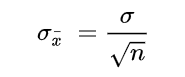
Therefore, the relationship between the standard error of the mean and the standard deviation is such that, for a given sample size, the standard error of the mean equals the standard deviation divided by the square root of the sample size.^[1] In other words, the standard error of the mean is a measure of the dispersion of sample means around the population mean.

In regression analysis, the term «standard error» refers either to the square root of the reduced chi-squared statistic or the standard error for a particular regression coefficient (as used in, say, confidence intervals).

Standard error of the sample mean[edit]

Exact value[edit]

Suppose a statistically independent sample of observations ${displaystyle x_{1},x_{2},ldots ,x_{n}}$ is taken from a statistical population with a standard deviation of sigma . The mean value calculated from the sample, , will have an associated standard error on the mean, ${displaystyle {sigma }_{bar {x}}}$ , given by:^[1]

${displaystyle {sigma }_{bar {x}} ={frac {sigma }{sqrt {n}}}}$

Practically this tells us that when trying to estimate the value of a population mean, due to the factor , reducing the error on the estimate by a factor of two requires acquiring four times as many observations in the sample; reducing it by a factor of ten requires a hundred times as many observations.

Estimate[edit]

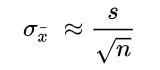
The standard deviation sigma of the population being sampled is seldom known. Therefore, the standard error of the mean is usually estimated by replacing sigma with the sample standard deviation $sigma _{x}$ instead:

${displaystyle {sigma }_{bar {x}} approx {frac {sigma _{x}}{sqrt {n}}}}$

As this is only an estimator for the true «standard error», it is common to see other notations here such as:

${displaystyle {widehat {sigma }}_{bar {x}}approx {frac {sigma _{x}}{sqrt {n}}}}$

or alternately ${displaystyle {s}_{bar {x}} approx {frac {s}{sqrt {n}}}}$

A common source of confusion occurs when failing to distinguish clearly between:

Accuracy of the estimator[edit]

When the sample size is small, using the standard deviation of the sample instead of the true standard deviation of the population will tend to systematically underestimate the population standard deviation, and therefore also the standard error. With n = 2, the underestimate is about 25%, but for n = 6, the underestimate is only 5%. Gurland and Tripathi (1971) provide a correction and equation for this effect.^[3] Sokal and Rohlf (1981) give an equation of the correction factor for small samples of n < 20.^[4] See unbiased estimation of standard deviation for further discussion.

Derivation[edit]

The standard error on the mean may be derived from the variance of a sum of independent random variables,^[5] given the definition of variance and some simple properties thereof. If ${displaystyle x_{1},x_{2},ldots ,x_{n}}$ are independent samples from a population with mean and standard deviation sigma , then we can define the total

${displaystyle T=(x_{1}+x_{2}+cdots +x_{n})}$

which due to the Bienaymé formula, will have variance

${displaystyle operatorname {Var} (T)approx {big (}operatorname {Var} (x_{1})+operatorname {Var} (x_{2})+cdots +operatorname {Var} (x_{n}){big )}=nsigma ^{2}.}$

where we’ve approximated the standard deviations, i.e., the uncertainties, of the measurements themselves with the best value for the standard deviation of the population. The mean of these measurements is simply given by

The variance of the mean is then

${displaystyle operatorname {Var} ({bar {x}})=operatorname {Var} left({frac {T}{n}}right)={frac {1}{n^{2}}}operatorname {Var} (T)={frac {1}{n^{2}}}nsigma ^{2}={frac {sigma ^{2}}{n}}.}$

The standard error is, by definition, the standard deviation of which is simply the square root of the variance:

${displaystyle sigma _{bar {x}}={sqrt {frac {sigma ^{2}}{n}}}={frac {sigma }{sqrt {n}}}}$

For correlated random variables the sample variance needs to be computed according to the Markov chain central limit theorem.

Independent and identically distributed random variables with random sample size[edit]

There are cases when a sample is taken without knowing, in advance, how many observations will be acceptable according to some criterion. In such cases, the sample size is a random variable whose variation adds to the variation of such that,

${displaystyle operatorname {Var} (T)=operatorname {E} (N)operatorname {Var} (X)+operatorname {Var} (N){big (}operatorname {E} (X){big )}^{2}}$

^[6]

If has a Poisson distribution, then with estimator . Hence the estimator of becomes ${displaystyle nS_{X}^{2}+n{bar {X}}^{2}}$ , leading the following formula for standard error:

${displaystyle operatorname {Standard~Error} ({bar {X}})={sqrt {frac {S_{X}^{2}+{bar {X}}^{2}}{n}}}}$

(since the standard deviation is the square root of the variance)

Student approximation when σ value is unknown[edit]

In many practical applications, the true value of σ is unknown. As a result, we need to use a distribution that takes into account that spread of possible σ’s.
When the true underlying distribution is known to be Gaussian, although with unknown σ, then the resulting estimated distribution follows the Student t-distribution. The standard error is the standard deviation of the Student t-distribution. T-distributions are slightly different from Gaussian, and vary depending on the size of the sample. Small samples are somewhat more likely to underestimate the population standard deviation and have a mean that differs from the true population mean, and the Student t-distribution accounts for the probability of these events with somewhat heavier tails compared to a Gaussian. To estimate the standard error of a Student t-distribution it is sufficient to use the sample standard deviation «s» instead of σ, and we could use this value to calculate confidence intervals.

Note: The Student’s probability distribution is approximated well by the Gaussian distribution when the sample size is over 100. For such samples one can use the latter distribution, which is much simpler.

Assumptions and usage[edit]

An example of how is used is to make confidence intervals of the unknown population mean. If the sampling distribution is normally distributed, the sample mean, the standard error, and the quantiles of the normal distribution can be used to calculate confidence intervals for the true population mean. The following expressions can be used to calculate the upper and lower 95% confidence limits, where is equal to the sample mean, is equal to the standard error for the sample mean, and 1.96 is the approximate value of the 97.5 percentile point of the normal distribution:

Upper 95% limit

{displaystyle ={bar {x}}+(operatorname {SE} times 1.96),}

and

Lower 95% limit

In particular, the standard error of a sample statistic (such as sample mean) is the actual or estimated standard deviation of the sample mean in the process by which it was generated. In other words, it is the actual or estimated standard deviation of the sampling distribution of the sample statistic. The notation for standard error can be any one of SE, SEM (for standard error of measurement or mean), or S_E.

Standard errors provide simple measures of uncertainty in a value and are often used because:

in many cases, if the standard error of several individual quantities is known then the standard error of some function of the quantities can be easily calculated;
when the probability distribution of the value is known, it can be used to calculate an exact confidence interval;
when the probability distribution is unknown, Chebyshev’s or the Vysochanskiï–Petunin inequalities can be used to calculate a conservative confidence interval; and
as the sample size tends to infinity the central limit theorem guarantees that the sampling distribution of the mean is asymptotically normal.

Standard error of mean versus standard deviation[edit]

In scientific and technical literature, experimental data are often summarized either using the mean and standard deviation of the sample data or the mean with the standard error. This often leads to confusion about their interchangeability. However, the mean and standard deviation are descriptive statistics, whereas the standard error of the mean is descriptive of the random sampling process. The standard deviation of the sample data is a description of the variation in measurements, while the standard error of the mean is a probabilistic statement about how the sample size will provide a better bound on estimates of the population mean, in light of the central limit theorem.^[7]

Put simply, the standard error of the sample mean is an estimate of how far the sample mean is likely to be from the population mean, whereas the standard deviation of the sample is the degree to which individuals within the sample differ from the sample mean.^[8] If the population standard deviation is finite, the standard error of the mean of the sample will tend to zero with increasing sample size, because the estimate of the population mean will improve, while the standard deviation of the sample will tend to approximate the population standard deviation as the sample size increases.

Extensions[edit]

Finite population correction (FPC)[edit]

The formula given above for the standard error assumes that the population is infinite. Nonetheless, it is often used for finite populations when people are interested in measuring the process that created the existing finite population (this is called an analytic study). Though the above formula is not exactly correct when the population is finite, the difference between the finite- and infinite-population versions will be small when sampling fraction is small (e.g. a small proportion of a finite population is studied). In this case people often do not correct for the finite population, essentially treating it as an «approximately infinite» population.

If one is interested in measuring an existing finite population that will not change over time, then it is necessary to adjust for the population size (called an enumerative study). When the sampling fraction (often termed f) is large (approximately at 5% or more) in an enumerative study, the estimate of the standard error must be corrected by multiplying by a »finite population correction» (a.k.a.: FPC):^[9]
^[10]

${displaystyle operatorname {FPC} ={sqrt {frac {N-n}{N-1}}}}$

which, for large N:

${displaystyle operatorname {FPC} approx {sqrt {1-{frac {n}{N}}}}={sqrt {1-f}}}$

to account for the added precision gained by sampling close to a larger percentage of the population. The effect of the FPC is that the error becomes zero when the sample size n is equal to the population size N.

This happens in survey methodology when sampling without replacement. If sampling with replacement, then FPC does not come into play.

Correction for correlation in the sample[edit]

Expected error in the mean of A for a sample of n data points with sample bias coefficient ρ. The unbiased standard error plots as the ρ = 0 diagonal line with log-log slope −½.

If values of the measured quantity A are not statistically independent but have been obtained from known locations in parameter space x, an unbiased estimate of the true standard error of the mean (actually a correction on the standard deviation part) may be obtained by multiplying the calculated standard error of the sample by the factor f:

$f={sqrt {frac {1+rho }{1-rho }}},$

where the sample bias coefficient ρ is the widely used Prais–Winsten estimate of the autocorrelation-coefficient (a quantity between −1 and +1) for all sample point pairs. This approximate formula is for moderate to large sample sizes; the reference gives the exact formulas for any sample size, and can be applied to heavily autocorrelated time series like Wall Street stock quotes. Moreover, this formula works for positive and negative ρ alike.^[11] See also unbiased estimation of standard deviation for more discussion.

References[edit]

^ ^a ^b ^c ^d Altman, Douglas G; Bland, J Martin (2005-10-15). «Standard deviations and standard errors». BMJ: British Medical Journal. 331 (7521): 903. doi:10.1136/bmj.331.7521.903. ISSN 0959-8138. PMC 1255808. PMID 16223828.
^ Everitt, B. S. (2003). The Cambridge Dictionary of Statistics. CUP. ISBN 978-0-521-81099-9.
^ Gurland, J; Tripathi RC (1971). «A simple approximation for unbiased estimation of the standard deviation». American Statistician. 25 (4): 30–32. doi:10.2307/2682923. JSTOR 2682923.
^ Sokal; Rohlf (1981). Biometry: Principles and Practice of Statistics in Biological Research (2nd ed.). p. 53. ISBN 978-0-7167-1254-1.
^ Hutchinson, T. P. (1993). Essentials of Statistical Methods, in 41 pages. Adelaide: Rumsby. ISBN 978-0-646-12621-0.
^ Cornell, J R, and Benjamin, C A, Probability, Statistics, and Decisions for Civil Engineers, McGraw-Hill, NY, 1970, ISBN 0486796094, pp. 178–9.
^ Barde, M. (2012). «What to use to express the variability of data: Standard deviation or standard error of mean?». Perspect. Clin. Res. 3 (3): 113–116. doi:10.4103/2229-3485.100662. PMC 3487226. PMID 23125963.
^ Wassertheil-Smoller, Sylvia (1995). Biostatistics and Epidemiology : A Primer for Health Professionals (Second ed.). New York: Springer. pp. 40–43. ISBN 0-387-94388-9.
^ Isserlis, L. (1918). «On the value of a mean as calculated from a sample». Journal of the Royal Statistical Society. 81 (1): 75–81. doi:10.2307/2340569. JSTOR 2340569. (Equation 1)
^ Bondy, Warren; Zlot, William (1976). «The Standard Error of the Mean and the Difference Between Means for Finite Populations». The American Statistician. 30 (2): 96–97. doi:10.1080/00031305.1976.10479149. JSTOR 2683803. (Equation 2)
^ Bence, James R. (1995). «Analysis of Short Time Series: Correcting for Autocorrelation». Ecology. 76 (2): 628–639. doi:10.2307/1941218. JSTOR 1941218.

Источник

The standard error of the estimate is a way to measure the accuracy of the predictions made by a regression model.

Often denoted σ_est, it is calculated as:

σ_est = √Σ(y – ŷ)²/n

where:

y: The observed value
ŷ: The predicted value
n: The total number of observations

The standard error of the estimate gives us an idea of how well a regression model fits a dataset. In particular:

The smaller the value, the better the fit.
The larger the value, the worse the fit.

For a regression model that has a small standard error of the estimate, the data points will be closely packed around the estimated regression line:

Conversely, for a regression model that has a large standard error of the estimate, the data points will be more loosely scattered around the regression line:

The following example shows how to calculate and interpret the standard error of the estimate for a regression model in Excel.

Example: Standard Error of the Estimate in Excel

Use the following steps to calculate the standard error of the estimate for a regression model in Excel.

Step 1: Enter the Data

First, enter the values for the dataset:

Step 2: Perform Linear Regression

Next, click the Data tab along the top ribbon. Then click the Data Analysis option within the Analyze group.

If you don’t see this option, you need to first load the Analysis ToolPak.

In the new window that appears, click Regression and then click OK.

In the new window that appears, fill in the following information:

Once you click OK, the regression output will appear:

We can use the coefficients from the regression table to construct the estimated regression equation:

ŷ = 13.367 + 1.693(x)

And we can see that the standard error of the estimate for this regression model turns out to be 6.006. In simple terms, this tells us that the average data point falls 6.006 units from the regression line.

We can use the estimated regression equation and the standard error of the estimate to construct a 95% confidence interval for the predicted value of a certain data point.

For example, suppose x is equal to 10. Using the estimated regression equation, we would predict that y would be equal to:

ŷ = 13.367 + 1.693*(10) = 30.297

And we can obtain the 95% confidence interval for this estimate by using the following formula:

95% C.I. = [ŷ – 1.96*σ_est, ŷ + 1.96*σ_est]

For our example, the 95% confidence interval would be calculated as:

95% C.I. = [ŷ – 1.96*σ_est, ŷ + 1.96*σ_est]
95% C.I. = [30.297 – 1.96*6.006, 30.297 + 1.96*6.006]
95% C.I. = [18.525, 42.069]

Additional Resources

How to Perform Simple Linear Regression in Excel
How to Perform Multiple Linear Regression in Excel
How to Create a Residual Plot in Excel

Источник

Download Article

The standard error of estimate is used to determine how well a straight line can describe values of a data set. When you have a collection of data from some measurement, experiment, survey or other source, you can create a line of regression to estimate additional data. With the standard error of estimate, you get a score that describes how good the regression line is.

1

Create a five column data table. Any statistical work is generally made easier by having your data in a concise format. A simple table serves this purpose very well. To calculate the standard error of estimate, you will be using five different measurements or calculations. Therefore, creating a five-column table is helpful. Label the five columns as follows:^[1]
2
Enter the data values for your measured data. After collecting your data, you will have pairs of data values. For these statistical calculations, the independent variable is labeled and the dependent, or resulting, variable is . Enter these values into the first two columns of your data table.^[2]
- The order of the data and the pairing is important for these calculations. You need to be careful to keep your paired data points together in order.
- For the sample calculations shown above, the data pairs are as follows:
  - (1,2)
  - (2,4)
  - (3,5)
  - (4,4)
  - (5,5)
Advertisement
3
Calculate a regression line. Using your data results, you will be able to calculate a regression line. This is also called a line of best fit or the least squares line. The calculation is tedious but can be done by hand. Alternatively, you can use a handheld graphing calculator or some online programs that will quickly calculate a best fit line using your data.^[3]
- For this article, it is assumed that you will have the regression line equation available or that it has been predicted by some prior means.
- For the sample data set in the image above, the regression line is $y^{{prime }}=0.6x+2.2$ .
4

Calculate predicted values from the regression line. Using the equation of that line, you can calculate predicted y-values for each x-value in your study, or for other theoretical x-values that you did not measure.^[4]

1
Calculate the error of each predicted value. In the fourth column of your data table, you will calculate and record the error of each predicted value. Specifically, subtract the predicted value ( $y^{{prime }}$ ) from the actual observed value ().^[5]
- For the data in the sample set, these calculations are as follows:
2
Calculate the squares of the errors. Take each value in the fourth column and square it by multiplying it by itself. Fill in these results in the final column of your data table.
- For the sample data set, these calculations are as follows:
3
Find the sum of the squared errors (SSE). The statistical value known as the sum of squared errors (SSE) is a useful step in finding standard deviation, variance and other measurements. To find the SSE from your data table, add the values in the fifth column of your data table.^[6]
- For this sample data set, this calculation is as follows:
4
Finalize your calculations. The Standard Error of the Estimate is the square root of the average of the SSE. It is generally represented with the Greek letter . Therefore, the first calculation is to divide the SSE score by the number of measured data points. Then, find the square root of that result.^[7]
- If the measured data represents an entire population, then you will find the average by dividing by N, the number of data points. However, if you are working with a smaller sample set of the population, then substitute N-2 in the denominator.
- For the sample data set in this article, we can assume that it is a sample set and not a population, just because there are only 5 data values. Therefore, calculate the Standard Error of the Estimate as follows:
5
Interpret your result. The Standard Error of the Estimate is a statistical figure that tells you how well your measured data relates to a theoretical straight line, the line of regression. A score of 0 would mean a perfect match, that every measured data point fell directly on the line. Widely scattered data will have a much higher score.^[8]
- With this small sample set, the standard error score of 0.894 is quite low and represents well organized data results.

Ask a Question

200 characters left

Include your email address to get a message when this question is answered.

Submit

Video

Thanks for submitting a tip for review!

References

About This Article

Article SummaryX

To calculate the standard error of estimate, create a five-column data table. In the first two columns, enter the values for your measured data, and enter the values from the regression line in the third column. In the fourth column, calculate the predicted values from the regression line using the equation from that line. These are the errors. Fill in the fifth column by multiplying each error by itself. Add together all of the values in column 5, then take the square root of that number to get the standard error of estimate. To learn how to organize the data pairs, keep reading!

Did this summary help you?

Thanks to all authors for creating a page that has been read 186,557 times.

Did this article help you?

Источник

Errors are of various types and impact the research process in different ways. Here’s a deep exploration of the standard error, the types, implications, formula, and how to interpret the values

What is a Standard Error?

The standard error is a statistical measure that accounts for the extent to which a sample distribution represents the population of interest using standard deviation. You can also think of it as the standard deviation of your sample in relation to your target population.

The standard error allows you to compare two similar measures in your sample data and population. For example, the standard error of the mean measures how far the sample mean (average) of the data is likely to be from the true population mean—the same applies to other types of standard errors.

Explore: Survey Errors To Avoid: Types, Sources, Examples, Mitigation

Why is Standard Error Important?

First, the standard error of a sample accounts for statistical fluctuation.

Researchers depend on this statistical measure to know how much sampling fluctuation exists in their sample data. In other words, it shows the extent to which a statistical measure varies from sample to population.

In addition, standard error serves as a measure of accuracy. Using standard error, a researcher can estimate the efficiency and consistency of a sample to know precisely how a sampling distribution represents a population.

How Many Types of Standard Error Exist?

There are five types of standard error which are:

Standard error of the mean
Standard error of measurement
Standard error of the proportion
Standard error of estimate
Residual Standard Error

1. Standard Error of the Mean (SEM)

The standard error of the mean accounts for the difference between the sample mean and the population mean. In other words, it quantifies how much variation is expected to be present in the sample mean that would be computed from every possible sample, of a given size, taken from the population.

How to Find SEM (With Formula)

SEM = Standard Deviation ÷ √n

Where;

n = sample size

Suppose that the standard deviation of observation is 15 with a sample size of 100. Using this formula, we can deduce the standard error of the mean as follows:

SEM = 15 ÷ √100

Standard Error of Mean in 1.5

2. Standard Error of Measurement

The standard error of measurement accounts for the consistency of scores within individual subjects in a test or examination.

This means it measures the extent to which estimated test or examination scores are spread around a true score.

A more formal way to look at it is through the 1985 lens of Aera, APA, and NCME. Here, they define a standard error as “the standard deviation of errors of measurement that is associated with the test scores for a specified group of test-takers….”

Read: 7 Types of Data Measurement Scales in Research

How to Find Standard Error of Measurement

Where;

rxx is the reliability of the test and is calculated as:

Rxx = S2T / S2X

Where;

S2T = variance of the true scores.

S2X = variance of the observed scores.

Suppose an organization has a reliability score of 0.4 and a standard deviation of 2.56. This means

SEm = 2.56 × √1–0.4 = 1.98

3. Standard Error of the Estimate

The standard error of the estimate measures the accuracy of predictions in sampling, research, and data collection. Specifically, it measures the distance that the observed values fall from the regression line which is the single line with the smallest overall distance from the line to the points.

How to Find Standard Error of the Estimate

The formula for standard error of the estimate is as follows:

Where;

σest is the standard error of the estimate;

Y is an actual score;

Y’ is a predicted score, and;

N is the number of pairs of scores.

The numerator is the sum of squared differences between the actual scores and the predicted scores.

4. Standard Error of Proportion

The standard of error of proportion in an observation is the difference between the sample proportion and the population proportion of your target audience. In more technical terms, this variable is the spread of the sample proportion about the population proportion.

How to Find Standard Error of the Proportion

The formula for calculating the standard error of the proportion is as follows:

Where;

P (hat) is equal to x ÷ n (with number of success x and the total number of observations of n)

5. Residual Standard Error

Residual standard error accounts for how well a linear regression model fits the observation in a systematic investigation. A linear regression model is simply a linear equation representing the relationship between two variables, and it helps you to predict similar variables.

How to Calculate Residual Standard Error

The formula for residual standard error is as follows:

Residual standard error = √Σ(y – ŷ)2/df

where:

y: The observed value

ŷ: The predicted value

df: The degrees of freedom, calculated as the total number of observations – total number of model parameters.

As you interpret your data, you should note that the smaller the residual standard error, the better a regression model fits a dataset, and vice versa.

How Do You Calculate Standard Error?

The formula for calculating standard error is as follows:

Where

σ – Standard deviation

n – Sample size, i.e., the number of observations in the sample

Here’s how this works in real-time.

Suppose the standard deviation of a sample is 1.5 with 4 as the sample size. This means:

Standard Error = 1.5 ÷ √4

That is; 1.5 ÷2 = 0.75

Alternatively, you can use a standard error calculator to speed up the process for larger data sets.

How to Interpret Standard Error Values

As stated earlier, researchers use the standard error to measure the reliability of observation. This means it allows you to compare how far a particular variable in the sample data is from the population of interest.

Calculating standard error is just one piece of the puzzle; you need to know how to interpret your data correctly and draw useful insights for your research. Generally, a small standard error is an indication that the sample mean is a more accurate reflection of the actual population mean, while a large standard error means the opposite.

Standard Error Example

Suppose you need to find the standard error of the mean of a data set using the following information:

Standard Deviation: 1.5

n = 13

Standard Error of the Mean = Standard Deviation ÷ √n

1.5 ÷ √13 = 0.42

How Should You Report the Standard Error?

After calculating the standard error of your observation, the next thing you should do is present this data as part of the numerous variables affecting your observation. Typically, researchers report the standard error alongside the mean or in a confidence interval to communicate the uncertainty around the mean.

Applications of Standard Error

The most common application of standard error are in statistics and economics. In statistics, standard error allows researchers to determine the confidence interval of their data sets, and in some cases, the margin of error. Researchers also use standard error in hypothesis testing and regression analysis.

FAQs About Standard Error

What Is the Difference Between Standard Deviation and Standard Error of the Mean?

The major difference between standard deviation and standard error of the mean is how they account for the differences between the sample data and the population of interest.

Researchers use standard deviation to measure the variability or dispersion of a data set to its mean. On the other hand, the standard error of the mean accounts for the difference between the mean of the data sample and that of the target population.

Something else to note here is that the standard error of a sample is always smaller than the corresponding standard deviation.

What Is The Symbol for Standard Error?

During calculation, the standard error is represented as σx̅.

Is Standard Error the Same as Margin of Error?

No. Margin of Error and standard error are not the same. Researchers use the standard error to measure the preciseness of an estimate of a population, meanwhile margin of error accounts for the degree of error in results received from random sampling surveys.

The standard error is calculated as s / √n where;

s: Sample standard deviation

n: Sample size

On the other hand, margin of error = z*(s/√n) where:

z: Z value that corresponds to a given confidence level

s: Sample standard deviation

n: Sample size

Источник

Correlation and Regression

Andrew F. Siegel, Michael R. Wagner, in Practical Business Statistics (Eighth Edition), 2022

The Standard Error of Estimate: How Large Are the Prediction Errors?

The standard error of estimate, denoted S_e here (but often denoted S in computer printouts), tells you approximately how large the prediction errors (residuals) are for your data set in the same units as Y. How well can you predict Y? The answer is to within about S_e above or below.¹⁶ Because you usually want your forecasts and predictions to be as accurate as possible, you would be glad to find a small value for S_e. You can interpret S_e as a standard deviation in the sense that if you have a normal distribution for the prediction errors, then you will expect about two-thirds of the data points to fall within a distance S_e either above or below the regression line. Also, about 95% of the data values should fall within 2S_e, and so forth. This is illustrated in Fig. 11.2.10 for the production cost example.

Fig. 11.2.10. The standard error of estimate, S_e, indicates approximately how much error you make when you use the predicted value for Y (on the least-squares line) instead of the actual value of Y. You may expect about two-thirds of the data points to be within S_e above or below the least-squares line for a data set with a normal linear relationship, such as this one.

The standard error of estimate may be found using the following formulas:

Standard Error of Estimate

Se=SY(1−r2)n−1n−2(forcomputation)=1n−2∑i=1n[Yi−(a+bXi)]2(forinterpretation)

The first formula shows how S_e is computed by reducing S_Y according to the correlation and sample size. Indeed, S_e will usually be smaller than S_Y because the line a + bX summarizes the relationship and therefore comes closer to the Y values than does the simpler summary, Y¯. The second formula shows how S_e can be interpreted as the estimated standard deviation of the residuals: The squared prediction errors are averaged by dividing by n − 2 (the appropriate number of degrees of freedom when two numbers, a and b, have been estimated), and the square root undoes the earlier squaring, giving you an answer in the same measurement units as Y.

For the production cost data, the correlation was found to be r = 0.869193, the variability in the individual cost numbers is S_Y = $389.6131, and the sample size is n = 18. The standard error of estimate is therefore

Se=SY(1−r2)n−1n−2=389.6131(1−0.8691932)18−118−2=389.6131(0.0244503)1716=389.61310.259785=$198.58

This tells you that, for a typical week, the actual cost was different from the predicted cost (on the least-squares line) by about $198.58. Although the least-squares prediction line takes full advantage of the relationship between cost and number produced, the predictions are far from perfect.

Read full chapter

URL:

https://www.sciencedirect.com/science/article/pii/B9780128200254000117

Detection of a Trend in Population Estimates

William L. Thompson, … Charles Gowan, in Monitoring Vertebrate Populations, 1998

5.2 VARIANCE COMPONENTS

In this section, we discuss sources of variation that must be considered to make inferences from data when trying to detect trends. Three sources of variation must be considered: sampling variation, temporal variation in the population dynamics process, and spatial variation in the dynamics of the population across space. The latter two sources often are referred to as process variation, i.e., variation in the population dynamics process associated with environmental variation (such as rainfall, temperature, community succession, fires, or elevation). Methods to separate process variation from sampling variation will be presented.

Detection of a trend in a population’s size requires at least two abundance estimates. For example, if the population size of Mexican spotted owls in Mesa Verde National Park is determined as 50 pairs in 1990, and as only 10 pairs in 1995, we would be concerned that a significant negative trend in the population exists during this time period, and that action must be taken to alleviate the trend. However, if the 1995 estimate was 40 pairs, we might still be concerned, but would be less confident that immediate action is required. Two sources of variation must be assessed before we are confident of our inference from these estimates.

The first source of variation is the uncertainty we have in our population estimates. We want to be sure that the two estimates are different, i.e., the difference between the two estimates is greater than would be expected from chance alone because of the sampling errors associated with each estimate. Typically, we present our uncertainty in our estimate as its variance, and use this variance to generate a confidence interval for our estimate. Suppose that the 1990 estimate of Nˆ90 = 50 pairs has a sampling variance of Vaˆr(Nˆ90)=25. Then, under the assumption of the estimate being normally distributed with a large sample size (i.e., large degrees of freedom), we would compute a 95% confidence interval as 50 ± 1.96 25, or 40.2–59.8. If the 1995 estimate was Nˆ95 = 40 with a sampling variance of Vâr(Nˆ95) = 20, then the 95% confidence interval for this estimate is 40 ± 1.96 20, or 31.2–48.8. Based on the overlap of the two confidence intervals (Fig. 5.2), we would conclude that by chance alone, these two estimates are probably not different. We also could compute a simple test as

Figure 5.2. The 95% confidence intervals plotted with the 1990 and 1995 population estimates.

(5.3)z=Nˆ90−Nˆ95Vaˆr(Nˆ90)+Vaˆr(Nˆ95),

which for this example results in z = 1.491, with a probability of observing a z statistic this large or larger of P = 0.136. Although we might be alarmed, the chances are that 13.6 times out of 100 we would observe this large of a change just by random chance.

A variation of the previous test is commonly conducted for several reasons: (1) we often are interested in the ratio of two population estimates (rather than the difference) because a ratio represents the rate of change of the population, (2) the variance of Nˆ is usually linked to its estimate by Vaˆr(Nˆ)=NˆC (e.g., Skalski and Robson, 1992, pp. 28–29), and (3) ln(Nˆ) is more likely to be normally distributed than Nˆ. Fortuitously, a log transformation provides some correction to all three of the above reasons and results in a more efficient statistical procedure. Because

(5.4)Var[ln(Nˆ)]=Var(Nˆ)Nˆ2,

we construct the z test as

(5.5)z=ln(Nˆ90)−ln(Nˆ95)Vaˆr[ln(Nˆ90)]+Vaˆr[ln(Nˆ95)]

to provide a more efficient (i.e., more powerful) test.

Suppose we had made a much more intensive effort in sampling the owl population, so that the sampling variances were one-half of the values observed (which would generally take about 4 times the effort). Thus, Vâr(Nˆ90) = 12.5 and Vâr(Nˆ95) = 10, giving a z statistic of 2.108 with probability value of P = 0.035. Now, we would conclude that the owl population was lower in 1995 than in 1990, and that this difference is unlikely due to variation in our samples, i.e., that an actual reduction in population size has taken place.

This leads us to the second variance component associated with determining whether a trend in the population is important. We would expect the size of the owl population (and any other population, for that matter) to fluctuate through time. How can we determine if this reduction is important? The answer lies in determining what the variation in the owl population has been for some period of time in the past, and then if the observed reduction is outside the range expected from this past fluctuation. Consider the example in Fig. 5.3, where the true population size (no sampling variation) is plotted. The population fluctuates around a mean of 50, but values more extreme than the range 40 to 60 are common. Note that a decline from 76 to 29 pairs occurred from 1984 to 1985, and that declines from over 50 pairs to under 40 pairs are fairly common occurrences. Thus, based on our previous example, a decline from 50 to 40 is not at all unreasonable given the past population dynamics of this hypothetical population.

Figure 5.3. Actual number of pairs of owls that exist each year. In reality, we never know these values, and can only estimate them.

To determine the level of change in population size that should receive our attention and suggest management action, we need to know something about the temporal variation in the population. The only way to estimate this variance component is to observe the population across a number of years. The exact number of years will depend on the magnitude of the temporal variation. Thus, if the population does not change much from year to year, a few observations will show this consistency. On the other hand, if the population fluctuates a lot, as in Fig. 5.3, many years of observations are needed to estimate the temporal variance. For the example in Fig. 5.3, we could compute the temporal variance as the variance of the 15 years. We find a variance of 265.7, or a standard deviation of 16.3 (Example 5.1). With a SD of 16.3, we would expect roughly 95% of the population values to be in the range of ±2 SD of the mean population size. This inference is based on the population being stable, i.e., not having an upward or downward trend, and being roughly normally distributed. For a normal distribution, 95% of the values lie in the interval ±2 SD of the mean. Therefore, a change of 2 SD, or 32.6, is not a particularly big change given the temporal variation observed over the 15-year period. Such a change should occur with probability greater than 1/20, or 0.05.

A complicating problem with estimating the temporal variance of a population’s size is that we are seldom allowed to observe the true value of the population size. Rather, we are required to sample the population, and hence only obtain an estimate of the population size each year, with its associated sampling variance. Thus, we would need to include the 95% confidence bars on the annual estimates. As a result of this uncertainty from our sampling procedure, we would conclude that many of the year-to-year changes were not really changes because the estimates were not different. This complication leads to a further problem. If we compute the variance with the usual formula when estimates of population size replace the actual population size shown in Fig. 5.3, we obtain a variance estimate larger than the true temporal variance because our sampling uncertainty is included in the variance. For low levels of sampling effort each year, we would have a high sampling variance associated with each estimate, and as a result, we would have a high variance across years. The noise associated with our low sampling intensity would suggest that the population is fluctuating widely, when in fact the population could be constant (i.e., temporal variance is zero), and the estimated changes in the population are just due to sampling variance.

This mixture of sampling and temporal variation becomes particularly important in population viability analysis (PVA). The objective of a PVA is to estimate the probability of extinction for a population, given current size, and some idea of the variation in the population dynamics (i.e., temporal variation). If our estimate of temporal variation includes sampling variation, and the level of effort to obtain the estimates is relatively low, the high sampling variation causes our naive estimate of temporal variation to be much too large. When we apply our PVA analysis with this inflated estimate of temporal variance, we conclude that the population is much more likely to go extinct than it really is, and hence the importance of separating sampling variation from process variation.

Typically, we estimate variance components with analysis of variance (ANOVA) procedures. For the example considered here, we would have to have at least two estimates of population size for a series of years to obtain valid estimates of sampling and temporal variation. Further, typical ANOVA techniques assume that the sampling variation is constant, and so do not account for differences in levels of effort, or the fact that sampling variance is usually a function of population size. For our example, we have an estimate of sampling variance for each of our estimates, obtained from the population estimation methods considered in this manual. That is, capture–recapture, mark–resight, line transects, removal methods, and quadrat counts all produce estimates of sampling variation. Thus, we do not want to estimate sampling variation by obtaining replicate estimates, but want to use the available estimate. Therefore, we present a method of moments estimator developed in Burnham et al. (1987, Part 5). Skalski and Robson (1992, Chapter 2) also present a similar procedure, but do not develop the weighted estimator presented here.

Example 5.1 Population Size, Estimates, Standard Error of the Estimates, and Confidence Intervals for Owl Pairs in Fig. 5.3

			Standard
Year	Population	Estimate	error	Lower 95% CI	Upper 95% CI
1980	44	40.04	5.926	28.42	51.66
1981	48	50.51	11.004	28.94	72.08
1982	61	61.36	15.278	31.42	91.31
1983	48	47.6	11.062	25.92	69.28
1984	76	95.51	18.988	58.3	132.72
1985	29	33.81	8.803	16.56	51.06
1986	60	34.39	5.804	23.01	45.76
1987	59	38.52	11.168	16.63	60.41
1988	76	84.57	21.312	42.8	126.34
1989	42	30.04	6.918	16.48	43.6
1990	29	20.29	7.529	5.54	35.05
1991	68	68.42	17.969	33.2	103.64
1992	42	45.51	13.225	19.6	71.44
1993	27	27.01	6.137	14.98	39.04
1994	72	71.12	14.511	42.67	99.56
1995	54	51.45	8.054	35.66	67.24

The variance of the n = 16 populations is 265.628, whereas the variance of the 16 estimates is 450.376. Sampling variation causes the estimates to have a larger variance than the actual population. The difference of these two variances is an estimate of the sampling variation, i.e., 450.376 – 265.628 = 184.748. The square root of 184.748 is 13.592, and is the approximate mean of the 16 reported standard errors.

To obtain an unbiased estimate of the temporal variance, we must remove the sampling variation from the estimate of the total variance. Define σtotal2 as the total variance, estimated for n = 16 estimates of owl pairs (Nˆi, i = 1980, …, 1995) as

(5.6)σˆtotal2=Σi=19801995(Nˆi−N¯)2(n−1)=Σi=19801995Nˆi2(Σi−19801985Nˆi)2n(n−1),

where the symbol indicates the estimate of the parameter. Thus, Nˆi are the estimates of the actual populations, N_i, and σˆtotal2 is an estimate of the total variance σˆi2 For each estimate, Nˆi, we also have an associated sampling variance, σˆi2. Then, a simple estimator of the temporal variance, σ²_time, is given by

(5.7)σˆtime2=σˆtotal2−Σi=19801995σˆi2n,

when we can assume that all of the sampling variances, σˆi2, are equal. The above equation corresponds to Eq. (2.6) of Skalski and Robson (1992). When the σˆi2 cannot all be assumed to be equal, a more complex calculation is required (Burnham et al., 1987, Section 4.3) because each estimate must be weighted by its sampling variance. We take as the weight of each estimate the reciprocal of the sum of temporal variance plus the sampling variance, 1/(σˆtime2+σˆi2). That is, Var(Nˆi)=σˆtime2+σˆi2, so wi=1/Var(Nˆi)=1/(σˆtime2+σˆi2). Then, the weighted total variance is computed as

(5.8)σˆtotal2=Σi=19801995wi(Nˆi−N¯)2(n−1)Σi=19801995wi

with the mean of the estimates now computed as a weighted mean,

(5.9)N¯=Σi=19801995wiNˆiΣi=19801995wi.

We now know that the theoretical variance N¯ is

(5.10)Var(N¯)=Var(Σi=19801995wiNˆiΣi=19801995wi)=1Σi=19801995wi

and the empirical variance estimator is Eq. (5.8). Setting these two equations equal,

(5.11)1Σi=19801995wi=Σi=19801995wi(Nˆi−N¯)2(n−1)Σi=19801995wi

(5.12)1=Σi=19801995wi(Nˆi−N¯)2(n−1).

Because we cannot solve for σˆtime2 directly, we have to use an iterative numerical approach to estimate σˆtime2 This procedure involves substituting values of σˆtime2 into Eq. (5.12) via the w_i until the two sides are equal. When both sides are the same, we have our estimate of σˆtime2. Using this estimate of σˆtime2, we can now decide what level of change in Nˆi to Nˆi+1 is important and deserves attention. If the change from a series of estimates is greater than 2σˆtime2, we may want to take action.

Typically, we do not have the luxury of enough background data to estimate σˆtime2, so we end up trying to evaluate whether a series of estimated population sizes is in fact signaling a decline in the population when both sampling and process variance are present. Note that just because we see a decline of the estimates for 3–4 consecutive years, we cannot be sure that the population is actually in a serious decline without knowledge of the mean population size and the temporal variation prior to the decline. Usually, however, we do not have good knowledge of the population size prior to some observed decline, and make a decision to act based on biological perceptions. Keep in mind the kinds of trends displayed in Fig. 5.1. Is the suggested trend part of a cycle, or are we observing a real change in population size? In this discussion, we have only considered temporal variation. A similar procedure can be used to separate spatial variation from sampling variation.

Read full chapter

URL:

https://www.sciencedirect.com/science/article/pii/B9780126889604500058

Multiple Regression

Andrew F. Siegel, Michael R. Wagner, in Practical Business Statistics (Eighth Edition), 2022

Typical Prediction Error: Standard Error of Estimate

Just as for simple regression, with only one X, the standard error of estimate indicates the approximate size of the prediction errors. For the magazine ads example, S_e = $106,072. This tells you that actual page costs for these magazines are typically within about $106,072 from the predicted page costs, in the sense of a standard deviation. That is, if the error distribution is normal, then you would expect about two-thirds of the actual page costs to be within S_e of the predicted page costs, about 95% to be within 2S_e, and so forth.

The standard error of estimate, S_e = $106,072, indicates the remaining variation in page costs after you have used the X variables (audience, percent male, and median income) in the regression equation to predict page costs for each magazine. Compare this to the ordinary univariate standard deviation, S_Y = $163,549, for the page costs, computed by ignoring all the other variables. This standard deviation, S_Y, indicates the remaining variation in page costs after you have used only Y¯ to predict the page costs for each magazine. Note that S_e = $106,072 is smaller than S_Y = $163,549; your errors are typically smaller if you use the regression equation instead of just Y¯ to predict page costs. This suggests that the X variables are helpful in explaining page costs.

Think of the situation this way. If you knew nothing of the X variables, you would use the average page costs (Y¯=$187,628) as your best guess, and you would be wrong by about S_Y = $163,549. But if you knew the audience, percent male readership, and median reader income, you could use the regression equation to find a prediction for page costs that would be wrong by only S_e = $106,072. This reduction in prediction error (from $163,549 to $106,072) is one of the helpful payoffs from running a regression analysis.

Read full chapter

URL:

https://www.sciencedirect.com/science/article/pii/B9780128200254000129

Multiple Regression

Gary Smith, in Essential Statistics, Regression, and Econometrics, 2012

Confidence Intervals for the Coefficients

If the error term is normally distributed and satisfies the four assumptions detailed in the simple regression chapter, the estimators are normally distributed with expected values equal to the parameters they estimate:

a∼N[α, standard deviation of a]bi∼N[βi, standard deviation of bi]

To compute the standard errors (the estimated standard deviations) of these estimators, we need to use the standard error of estimate (SEE) to estimate the standard deviation of the error term:

(10.3)SEE=∑(Y−Y^)2n−(k+1)

Because n observations are used to estimate k + 1 parameters, we have n − (k + 1) degrees of freedom. After choosing a confidence level, such as 95 percent, we use the t distribution with n − (k + 1) degrees of freedom to determine the value t* that corresponds to this probability. The confidence interval for each coefficient is equal to the estimate plus or minus the requisite number of standard errors:

(10.4)a±t*(standard error ofa)bi±t*(standard error ofbi)

For our consumption function, statistical software calculates SEE = 59.193 and these standard errors:

standard error ofa=27.327standard error ofb1=0.019standard error ofb2=0.003

With 49 observations and 2 explanatory variables, we have 49 − (2 + 1) = 46 degrees of freedom. Table A.2 gives t* = 2.013 for a 95 percent confidence interval, so that 95 percent confidence intervals are

α:a±t*(standard error ofa)=−110.126±2.013(27.327)=−110.126±55.010β1:b1±t*(standard error ofb1)=0.798±2.013(0.019)=0.798±0.039β2:b2±t*(standard error ofb2)=0.026±2.013(0.003)=0.026±0.006

Read full chapter

URL:

https://www.sciencedirect.com/science/article/pii/B9780123822215000106

Multiple Regression

Gary Smith, in Essential Statistics, Regression, and Econometrics (Second Edition), 2015

Confidence Intervals for the Coefficients

a∼N[α,standarddeviationofa]bi∼N[βistandarddeviationofbi]

To compute the standard errors (the estimated standard deviations) of these estimators, we need to use the standard error of estimate (SEE) to estimate the standard deviation of the error term:

(10.5)SEE=∑(y−yˆ)2n−(k+1)

Because n observations are used to estimate k + 1 parameters, we have n − (k + 1) degrees of freedom. After choosing a confidence level, such as 95 percent, we use the t distribution with n − (k + 1) degrees of freedom to determine the value t^∗ that corresponds to this probability. The confidence interval for each coefficient is equal to the estimate plus or minus the requisite number of standard errors:

(10.6)a±t∗(standarderrorofa)bi±t∗(standarderrorofbi)

For our consumption function, statistical software calculates SEE = 59.193 and these standard errors:

standarderrorofa=27.327standarderrorofb1=0.019standarderrorofb2=0.003

With 49 observations and two explanatory variables, we have 49 − (2 + 1) = 46 degrees of freedom. Table A.2 gives t^∗ = 2.013 for a 95 percent confidence interval, so that 95 percent confidence intervals are:

α:a±t∗(standarderrorofa)=−110.126±2.013(27.327)=−110.126±55.010β1:b1±t∗(standarderrorofb1)=0.798±2.013(0.019)=0.798±0.039β2:b2±t∗(standarderrorofb2)=0.026±2.013(0.003)=0.026±0.006

Read full chapter

URL:

https://www.sciencedirect.com/science/article/pii/B9780128034590000108

Simple Regression

Gary Smith, in Essential Statistics, Regression, and Econometrics (Second Edition), 2015

Abstract

The simple regression model assumes a linear relationship, Y = α + βX + ε, between a dependent variable Y and an explanatory variable X, with the error term ε encompassing omitted factors. The least squares estimates a and b minimize the sum of squared errors when the fitted line is used to predict the observed values of Y. The standard error of estimate (SEE) is our estimate of the standard deviation of the error term. The standard errors of the estimates a and b can be used to construct confidence intervals for α and β and test null hypotheses, most often that the value of β is zero (Y and X are not linearly related). The coefficient of determination R² compares the model’s sum of the squared prediction errors to the sum of the squared deviations of Y about its mean, and can be interpreted as the fraction of the variation in the dependent variable that is explained by the regression model. The correlation coefficient is equal to the square root of R².

Read full chapter

URL:

https://www.sciencedirect.com/science/article/pii/B978012803459000008X

Bootstrap Method

K. Singh, M. Xie, in International Encyclopedia of Education (Third Edition), 2010

Approximating Standard Error of a Sample Estimate

Let us suppose, information is sought about a population parameter θ. Suppose θˆ is a sample estimator of θ based on a random sample of size n, that is, θˆ is a function of the data (X₁, X₂, …,X_n). In order to estimate standard error of θˆ, as the sample varies over the class of all possible samples, one has the following simple bootstrap approach.

Computeθ1*,θ2*,…,θN*, using the same computing formula as the one used for θˆ, but now base it on N different bootstrap samples (each of size n). A crude recommendation for the size N could be N = n² (in our judgment), unless n² is too large. In that case, it could be reduced to an acceptable size, say nlogen. One defines

SEB(θˆ)=[(1/N)∑i=1N(θi*−θˆ)2]1/2

following the philosophy of bootstrap: replace the population by the empirical population.

An older resampling technique used for this purpose is Jackknife, though bootstrap is more widely applicable. The famous example where Jackknife fails while bootstrap is still useful is that of θˆ = the sample median.

Read full chapter

URL:

https://www.sciencedirect.com/science/article/pii/B9780080448947013099

Pearson, Karl

M. Eileen Magnello, in Encyclopedia of Social Measurement, 2005

The Biometric School

Although Pearson’s success in attracting such large audiences in his Gresham lectures may have played a role in encouraging him to further develop his work in biometry, he resigned from the Gresham Lectureship due to his doctor’s recommendation. Following the success of his Gresham lectures, Pearson began to teach statistics to students at UCL in October 1894. Not only did Galton’s work on his law of ancestral heredity enable Pearson to devise the mathematical properties of the product– moment correlation coefficient (which measures the relationship between two continuous variables) and simple regression (used for the linear prediction between two continuous variables) but also Galton’s ideas led to Pearson’s introduction of multiple correlation and part correlation coefficients, multiple regression and the standard error of estimate (for regression), and the coefficient of variation. By then, Galton had determined graphically the idea of correlation and regression for the normal distribution only. Because Galton’s procedure for measuring correlation involved measuring the slope of the regression line (which was a measure of regression instead), Pearson kept Galton’s “r” to symbolize correlation. Pearson later used the letter b (from the equation for a straight line) to symbolize regression. After Weldon had seen a copy of Pearson’s 1896 paper on correlation, he suggested to Pearson that he should extend the range for correlation from 0 to +1 (as used by Galton) so that it would include all values from −1 to +1.

Pearson achieved a mathematical resolution of multiple correlation and multiple regression, adumbrated in Galton’s law of ancestral heredity in 1885, in his seminal paper Regression, Heredity, and Panmixia in 1896, when he introduced matrix algebra into statistical theory. (Arthur Cayley, who taught at Cambridge when Pearson was a student, created matrix algebra by his discovery of the theory of invariants during the mid-19th century.) Pearson’s theory of multiple regression became important to his work on Mendel in 1904 when he advocated a synthesis of Mendelism and biometry. In the same paper, Pearson also introduced the following statistical methods: eta (η) as a measure for a curvilinear relationship, the standard error of estimate, multiple regression, and multiple and part correlation. He also devised the coefficient of variation as a measure of the ratio of a standard deviation to the corresponding mean expressed as a percentage.

By the end of the 19th century, he began to consider the relationship between two discrete variables, and from 1896 to 1911 Pearson devised more than 18 methods of correlation. In 1900, he devised the tetrachoric correlation and the phi coefficient for dichotomous variables. The tetrachoric correlation requires that both X and Y represent continuous, normally distributed, and linearly related variables, whereas the phi coefficient was designed for so-called point distributions, which implies that the two classes have two point values or merely represent some qualitative attribute. Nine years later, he devised the biserial correlation, where one variable is continuous and the other is discontinuous. With his son Egon, he devised the polychoric correlation in 1922 (which is very similar to canonical correlation today). Although not all of Pearson’s correlational methods have survived him, a number of these methods are still the principal tools used by psychometricians for test construction. Following the publication of his first three statistical papers in Philosophical Transactions of the Royal Society, Pearson was elected a fellow of the Royal Society in 1896. He was awarded the Darwin Medal from the Royal Society in 1898.

Read full chapter

URL:

https://www.sciencedirect.com/science/article/pii/B0123693985002280

Источник

What Is the Standard Error?

The standard error (SE) of a statistic is the approximate standard deviation of a statistical sample population.

The standard error is a statistical term that measures the accuracy with which a sample distribution represents a population by using standard deviation. In statistics, a sample mean deviates from the actual mean of a population; this deviation is the standard error of the mean.

Key Takeaways

The standard error (SE) is the approximate standard deviation of a statistical sample population.
The standard error describes the variation between the calculated mean of the population and one which is considered known, or accepted as accurate.
The more data points involved in the calculations of the mean, the smaller the standard error tends to be.

Standard Error

Understanding Standard Error

The term «standard error» is used to refer to the standard deviation of various sample statistics, such as the mean or median. For example, the «standard error of the mean» refers to the standard deviation of the distribution of sample means taken from a population. The smaller the standard error, the more representative the sample will be of the overall population.

The relationship between the standard error and the standard deviation is such that, for a given sample size, the standard error equals the standard deviation divided by the square root of the sample size. The standard error is also inversely proportional to the sample size; the larger the sample size, the smaller the standard error because the statistic will approach the actual value.

The standard error is considered part of inferential statistics. It represents the standard deviation of the mean within a dataset. This serves as a measure of variation for random variables, providing a measurement for the spread. The smaller the spread, the more accurate the dataset.

Standard error and standard deviation are measures of variability, while central tendency measures include mean, median, etc.

Formula and Calculation of Standard Error

The standard error of an estimate can be calculated as the standard deviation divided by the square root of the sample size:

SE = σ / √n

where

σ = the population standard deviation
√n = the square root of the sample size

If the population standard deviation is not known, you can substitute the sample standard deviation, s, in the numerator to approximate the standard error.

Requirements for Standard Error

When a population is sampled, the mean, or average, is generally calculated. The standard error can include the variation between the calculated mean of the population and one which is considered known, or accepted as accurate. This helps compensate for any incidental inaccuracies related to the gathering of the sample.

In cases where multiple samples are collected, the mean of each sample may vary slightly from the others, creating a spread among the variables. This spread is most often measured as the standard error, accounting for the differences between the means across the datasets.

The more data points involved in the calculations of the mean, the smaller the standard error tends to be. When the standard error is small, the data is said to be more representative of the true mean. In cases where the standard error is large, the data may have some notable irregularities.

The standard deviation is a representation of the spread of each of the data points. The standard deviation is used to help determine the validity of the data based on the number of data points displayed at each level of standard deviation. Standard errors function more as a way to determine the accuracy of the sample or the accuracy of multiple samples by analyzing deviation within the means.

Standard Error vs. Standard Deviation

The standard error normalizes the standard deviation relative to the sample size used in an analysis. Standard deviation measures the amount of variance or dispersion of the data spread around the mean. The standard error can be thought of as the dispersion of the sample mean estimations around the true population mean. As the sample size becomes larger, the standard error will become smaller, indicating that the estimated sample mean value better approximates the population mean.

Example of Standard Error

Say that an analyst has looked at a random sample of 50 companies in the S&P 500 to understand the association between a stock’s P/E ratio and subsequent 12-month performance in the market. Assume that the resulting estimate is -0.20, indicating that for every 1.0 point in the P/E ratio, stocks return 0.2% poorer relative performance. In the sample of 50, the standard deviation was found to be 1.0.

The standard error is thus:

SE = 1.0/√50 = 1/7.07 = 0.141

Therefore, we would report the estimate as -0.20% ± 0.14, giving us a confidence interval of (-0.34 — -0.06). The true mean value of the association of the P/E on returns of the S&P 500 would therefore fall within that range with a high degree of probability.

Say now that we increase the sample of stocks to 100 and find that the estimate changes slightly from -0.20 to -0.25, and the standard deviation falls to 0.90. The new standard error would thus be:

SE = 0.90/√100 = 0.90/10 = 0.09.

The resulting confidence interval becomes -0.25 ± 0.09 = (-0.34 — -0.16), which is a tighter range of values.

What Is Meant by Standard Error?

Standard error is intuitively the standard deviation of the sampling distribution. In other words, it depicts how much disparity there is likely to be in a point estimate obtained from a sample relative to the true population mean.

What Is a Good Standard Error?

Standard error measures the amount of discrepancy that can be expected in a sample estimate compared to the true value in the population. Therefore, the smaller the standard error the better. In fact, a standard error of zero (or close to it) would indicate that the estimated value is exactly the true value.

How Do You Find the Standard Error?

The standard error takes the standard deviation and divides it by the square root of the sample size. Many statistical software packages automatically compute standard errors.

The Bottom Line

The standard error (SE) measures the dispersion of estimated values obtained from a sample around the true value to be found in the population. Statistical analysis and inference often involves drawing samples and running statistical tests to determine associations and correlations between variables. The standard error thus tells us with what degree of confidence we can expect the estimated value to approximate the population value.

Источник

A mathematical tool used in statistics to measure variability

What is Standard Error?

Standard error is a mathematical tool used in statistics to measure variability. It enables one to arrive at an estimation of what the standard deviation of a given sample is. It is commonly known by its abbreviated form – SE.

Standard error is used to estimate the efficiency, accuracy, and consistency of a sample. In other words, it measures how precisely a sampling distribution represents a population.

It can be applied in statistics and economics. It is especially useful in the field of econometrics, where researchers use it in performing regression analyses and hypothesis testing. It is also used in inferential statistics, where it forms the basis for the construction of the confidence intervals.

Some commonly used measures in the field of statistics include:

Standard error of the mean (SEM)
Standard error of the variance
Standard error of the median
Standard error of a regression coefficient

Calculating Standard Error of the Mean (SEM)

The SEM is calculated using the following formula:

Where:

σ – Population standard deviation
n – Sample size, i.e., the number of observations in the sample

In a situation where statisticians are ignorant of the population standard deviation, they use the sample standard deviation as the closest replacement. SEM can then be calculated using the following formula. One of the primary assumptions here is that observations in the sample are statistically independent.

Where:

s – Sample standard deviation
n – Sample size, i.e., the number of observations in the sample

Importance of Standard Error

When a sample of observations is extracted from a population and the sample mean is calculated, it serves as an estimate of the population mean. Almost certainly, the sample mean will vary from the actual population mean. It will aid the statistician’s research to identify the extent of the variation. It is where the standard error of the mean comes into play.

When several random samples are extracted from a population, the standard error of the mean is essentially the standard deviation of different sample means from the population mean.

However, multiple samples may not always be available to the statistician. Fortunately, the standard error of the mean can be calculated from a single sample itself. It is calculated by dividing the standard deviation of the observations in the sample by the square root of the sample size.

Relationship between SEM and the Sample Size

Intuitively, as the sample size increases, the sample becomes more representative of the population.

For example, consider the marks of 50 students in a class in a mathematics test. Two samples A and B of 10 and 40 observations, respectively, are extracted from the population. It is logical to assert that the average marks in sample B will be closer to the average marks of the whole class than the average marks in sample A.

Thus, the standard error of the mean in sample B will be smaller than that in sample A. The standard error of the mean will approach zero with the increasing number of observations in the sample, as the sample becomes more and more representative of the population, and the sample mean approaches the actual population mean.

It is evident from the mathematical formula of the standard error of the mean that it is inversely proportional to the sample size. It can be verified using the SEM formula that if the sample size increases from 10 to 40 (becomes four times), the standard error will be half as big (reduces by a factor of 2).

Standard Deviation vs. Standard Error of the Mean

Standard deviation and standard error of the mean are both statistical measures of variability. While the standard deviation of a sample depicts the spread of observations within the given sample regardless of the population mean, the standard error of the mean measures the degree of dispersion of sample means around the population mean.

Standard error of the sample mean[edit]

Exact value[edit]

Estimate[edit]

Accuracy of the estimator[edit]

Derivation[edit]

Independent and identically distributed random variables with random sample size[edit]

Student approximation when σ value is unknown[edit]

Assumptions and usage[edit]

Standard error of mean versus standard deviation[edit]

Extensions[edit]

Finite population correction (FPC)[edit]

Correction for correlation in the sample[edit]

See also[edit]

References[edit]

Example: Standard Error of the Estimate in Excel

Additional Resources

Video

References

About This Article

Did this article help you?

What is a Standard Error?

Why is Standard Error Important?

How Many Types of Standard Error Exist?

1. Standard Error of the Mean (SEM)

2. Standard Error of Measurement

3. Standard Error of the Estimate

4. Standard Error of Proportion

5. Residual Standard Error

How Do You Calculate Standard Error?

How to Interpret Standard Error Values

Standard Error Example

How Should You Report the Standard Error?

Applications of Standard Error

FAQs About Standard Error

Correlation and Regression

The Standard Error of Estimate: How Large Are the Prediction Errors?

Standard Error of Estimate

Detection of a Trend in Population Estimates

5.2 VARIANCE COMPONENTS

Example 5.1 Population Size, Estimates, Standard Error of the Estimates, and Confidence Intervals for Owl Pairs in Fig. 5.3

Multiple Regression

Typical Prediction Error: Standard Error of Estimate

Multiple Regression

Confidence Intervals for the Coefficients

Multiple Regression

Confidence Intervals for the Coefficients

Simple Regression

Abstract

Bootstrap Method

Approximating Standard Error of a Sample Estimate

Pearson, Karl

The Biometric School

What Is the Standard Error?

Key Takeaways

Standard Error

Understanding Standard Error

Formula and Calculation of Standard Error

Requirements for Standard Error

Standard Error vs. Standard Deviation

Example of Standard Error

What Is Meant by Standard Error?

What Is a Good Standard Error?

How Do You Find the Standard Error?

The Bottom Line

What is Standard Error?

Calculating Standard Error of the Mean (SEM)

<img decoding="async" onError="javascript: wp_broken_images = window.wp_broken_images || function(){}; wp_broken_images(this);" loading="lazy" src="https://cdn.corporatefinanceinstitute.com/assets/standard-error1.png" alt="Standard Error - Formula" width="200" height="83" />

Importance of Standard Error

Relationship between SEM and the Sample Size

Standard Deviation vs. Standard Error of the Mean

Related Readings