Standard error statistics

From Wikipedia, the free encyclopedia

The standard error (SE)^[1] of a statistic (usually an estimate of a parameter) is the standard deviation of its sampling distribution^[2] or an estimate of that standard deviation. If the statistic is the sample mean, it is called the standard error of the mean (SEM).^[1]

The sampling distribution of a mean is generated by repeated sampling from the same population and recording of the sample means obtained. This forms a distribution of different means, and this distribution has its own mean and variance. Mathematically, the variance of the sampling mean distribution obtained is equal to the variance of the population divided by the sample size. This is because as the sample size increases, sample means cluster more closely around the population mean.

Therefore, the relationship between the standard error of the mean and the standard deviation is such that, for a given sample size, the standard error of the mean equals the standard deviation divided by the square root of the sample size.^[1] In other words, the standard error of the mean is a measure of the dispersion of sample means around the population mean.

In regression analysis, the term «standard error» refers either to the square root of the reduced chi-squared statistic or the standard error for a particular regression coefficient (as used in, say, confidence intervals).

Standard error of the sample mean[edit]

Exact value[edit]

Suppose a statistically independent sample of observations is taken from a statistical population with a standard deviation of . The mean value calculated from the sample, , will have an associated standard error on the mean, , given by:^[1]

.

Practically this tells us that when trying to estimate the value of a population mean, due to the factor , reducing the error on the estimate by a factor of two requires acquiring four times as many observations in the sample; reducing it by a factor of ten requires a hundred times as many observations.

Estimate[edit]

The standard deviation of the population being sampled is seldom known. Therefore, the standard error of the mean is usually estimated by replacing with the sample standard deviation instead:

.

As this is only an estimator for the true «standard error», it is common to see other notations here such as:

  or alternately   .

A common source of confusion occurs when failing to distinguish clearly between:

Accuracy of the estimator[edit]

When the sample size is small, using the standard deviation of the sample instead of the true standard deviation of the population will tend to systematically underestimate the population standard deviation, and therefore also the standard error. With n = 2, the underestimate is about 25%, but for n = 6, the underestimate is only 5%. Gurland and Tripathi (1971) provide a correction and equation for this effect.^[3] Sokal and Rohlf (1981) give an equation of the correction factor for small samples of n < 20.^[4] See unbiased estimation of standard deviation for further discussion.

Derivation[edit]

The standard error on the mean may be derived from the variance of a sum of independent random variables,^[5] given the definition of variance and some simple properties thereof. If are independent samples from a population with mean and standard deviation , then we can define the total

which due to the Bienaymé formula, will have variance

where we’ve approximated the standard deviations, i.e., the uncertainties, of the measurements themselves with the best value for the standard deviation of the population. The mean of these measurements is simply given by

.

The variance of the mean is then

The standard error is, by definition, the standard deviation of which is simply the square root of the variance:

.

For correlated random variables the sample variance needs to be computed according to the Markov chain central limit theorem.

Independent and identically distributed random variables with random sample size[edit]

There are cases when a sample is taken without knowing, in advance, how many observations will be acceptable according to some criterion. In such cases, the sample size is a random variable whose variation adds to the variation of such that,

^[6]

If has a Poisson distribution, then with estimator . Hence the estimator of becomes , leading the following formula for standard error:

(since the standard deviation is the square root of the variance)

Student approximation when σ value is unknown[edit]

In many practical applications, the true value of σ is unknown. As a result, we need to use a distribution that takes into account that spread of possible σ’s.
When the true underlying distribution is known to be Gaussian, although with unknown σ, then the resulting estimated distribution follows the Student t-distribution. The standard error is the standard deviation of the Student t-distribution. T-distributions are slightly different from Gaussian, and vary depending on the size of the sample. Small samples are somewhat more likely to underestimate the population standard deviation and have a mean that differs from the true population mean, and the Student t-distribution accounts for the probability of these events with somewhat heavier tails compared to a Gaussian. To estimate the standard error of a Student t-distribution it is sufficient to use the sample standard deviation «s» instead of σ, and we could use this value to calculate confidence intervals.

Note: The Student’s probability distribution is approximated well by the Gaussian distribution when the sample size is over 100. For such samples one can use the latter distribution, which is much simpler.

Assumptions and usage[edit]

An example of how is used is to make confidence intervals of the unknown population mean. If the sampling distribution is normally distributed, the sample mean, the standard error, and the quantiles of the normal distribution can be used to calculate confidence intervals for the true population mean. The following expressions can be used to calculate the upper and lower 95% confidence limits, where is equal to the sample mean, is equal to the standard error for the sample mean, and 1.96 is the approximate value of the 97.5 percentile point of the normal distribution:

Upper 95% limit and

Lower 95% limit

In particular, the standard error of a sample statistic (such as sample mean) is the actual or estimated standard deviation of the sample mean in the process by which it was generated. In other words, it is the actual or estimated standard deviation of the sampling distribution of the sample statistic. The notation for standard error can be any one of SE, SEM (for standard error of measurement or mean), or S_E.

Standard errors provide simple measures of uncertainty in a value and are often used because:

• in many cases, if the standard error of several individual quantities is known then the standard error of some function of the quantities can be easily calculated;
• when the probability distribution of the value is known, it can be used to calculate an exact confidence interval;
• when the probability distribution is unknown, Chebyshev’s or the Vysochanskiï–Petunin inequalities can be used to calculate a conservative confidence interval; and
• as the sample size tends to infinity the central limit theorem guarantees that the sampling distribution of the mean is asymptotically normal.

Standard error of mean versus standard deviation[edit]

In scientific and technical literature, experimental data are often summarized either using the mean and standard deviation of the sample data or the mean with the standard error. This often leads to confusion about their interchangeability. However, the mean and standard deviation are descriptive statistics, whereas the standard error of the mean is descriptive of the random sampling process. The standard deviation of the sample data is a description of the variation in measurements, while the standard error of the mean is a probabilistic statement about how the sample size will provide a better bound on estimates of the population mean, in light of the central limit theorem.^[7]

Put simply, the standard error of the sample mean is an estimate of how far the sample mean is likely to be from the population mean, whereas the standard deviation of the sample is the degree to which individuals within the sample differ from the sample mean.^[8] If the population standard deviation is finite, the standard error of the mean of the sample will tend to zero with increasing sample size, because the estimate of the population mean will improve, while the standard deviation of the sample will tend to approximate the population standard deviation as the sample size increases.

Extensions[edit]

Finite population correction (FPC)[edit]

The formula given above for the standard error assumes that the population is infinite. Nonetheless, it is often used for finite populations when people are interested in measuring the process that created the existing finite population (this is called an analytic study). Though the above formula is not exactly correct when the population is finite, the difference between the finite- and infinite-population versions will be small when sampling fraction is small (e.g. a small proportion of a finite population is studied). In this case people often do not correct for the finite population, essentially treating it as an «approximately infinite» population.

If one is interested in measuring an existing finite population that will not change over time, then it is necessary to adjust for the population size (called an enumerative study). When the sampling fraction (often termed f) is large (approximately at 5% or more) in an enumerative study, the estimate of the standard error must be corrected by multiplying by a »finite population correction» (a.k.a.: FPC):^[9]
[10]

which, for large N:

to account for the added precision gained by sampling close to a larger percentage of the population. The effect of the FPC is that the error becomes zero when the sample size n is equal to the population size N.

This happens in survey methodology when sampling without replacement. If sampling with replacement, then FPC does not come into play.

Correction for correlation in the sample[edit]

If values of the measured quantity A are not statistically independent but have been obtained from known locations in parameter space x, an unbiased estimate of the true standard error of the mean (actually a correction on the standard deviation part) may be obtained by multiplying the calculated standard error of the sample by the factor f:

where the sample bias coefficient ρ is the widely used Prais–Winsten estimate of the autocorrelation-coefficient (a quantity between −1 and +1) for all sample point pairs. This approximate formula is for moderate to large sample sizes; the reference gives the exact formulas for any sample size, and can be applied to heavily autocorrelated time series like Wall Street stock quotes. Moreover, this formula works for positive and negative ρ alike.^[11] See also unbiased estimation of standard deviation for more discussion.

See also[edit]

• Illustration of the central limit theorem
• Margin of error
• Probable error
• Standard error of the weighted mean
• Sample mean and sample covariance
• Standard error of the median
• Variance

References[edit]

What Is the Standard Error?

The standard error (SE) of a statistic is the approximate standard deviation of a statistical sample population.

The standard error is a statistical term that measures the accuracy with which a sample distribution represents a population by using standard deviation. In statistics, a sample mean deviates from the actual mean of a population; this deviation is the standard error of the mean.

Understanding Standard Error

The term «standard error» is used to refer to the standard deviation of various sample statistics, such as the mean or median. For example, the «standard error of the mean» refers to the standard deviation of the distribution of sample means taken from a population. The smaller the standard error, the more representative the sample will be of the overall population.

The relationship between the standard error and the standard deviation is such that, for a given sample size, the standard error equals the standard deviation divided by the square root of the sample size. The standard error is also inversely proportional to the sample size; the larger the sample size, the smaller the standard error because the statistic will approach the actual value.

The standard error is considered part of inferential statistics. It represents the standard deviation of the mean within a dataset. This serves as a measure of variation for random variables, providing a measurement for the spread. The smaller the spread, the more accurate the dataset.

Formula and Calculation of Standard Error

The standard error of an estimate can be calculated as the standard deviation divided by the square root of the sample size:

SE = σ / √n

where

• σ = the population standard deviation
• √n = the square root of the sample size

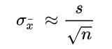
If the population standard deviation is not known, you can substitute the sample standard deviation, s, in the numerator to approximate the standard error.

Requirements for Standard Error 

When a population is sampled, the mean, or average, is generally calculated. The standard error can include the variation between the calculated mean of the population and one which is considered known, or accepted as accurate. This helps compensate for any incidental inaccuracies related to the gathering of the sample.

In cases where multiple samples are collected, the mean of each sample may vary slightly from the others, creating a spread among the variables. This spread is most often measured as the standard error, accounting for the differences between the means across the datasets.

The more data points involved in the calculations of the mean, the smaller the standard error tends to be. When the standard error is small, the data is said to be more representative of the true mean. In cases where the standard error is large, the data may have some notable irregularities.

The standard deviation is a representation of the spread of each of the data points. The standard deviation is used to help determine the validity of the data based on the number of data points displayed at each level of standard deviation. Standard errors function more as a way to determine the accuracy of the sample or the accuracy of multiple samples by analyzing deviation within the means.

Standard Error vs. Standard Deviation

The standard error normalizes the standard deviation relative to the sample size used in an analysis. Standard deviation measures the amount of variance or dispersion of the data spread around the mean. The standard error can be thought of as the dispersion of the sample mean estimations around the true population mean. As the sample size becomes larger, the standard error will become smaller, indicating that the estimated sample mean value better approximates the population mean.

Example of Standard Error

Say that an analyst has looked at a random sample of 50 companies in the S&P 500 to understand the association between a stock’s P/E ratio and subsequent 12-month performance in the market. Assume that the resulting estimate is -0.20, indicating that for every 1.0 point in the P/E ratio, stocks return 0.2% poorer relative performance. In the sample of 50, the standard deviation was found to be 1.0.

The standard error is thus:

SE = 1.0/√50 = 1/7.07 = 0.141

Therefore, we would report the estimate as -0.20% ± 0.14, giving us a confidence interval of (-0.34 — -0.06). The true mean value of the association of the P/E on returns of the S&P 500 would therefore fall within that range with a high degree of probability.

Say now that we increase the sample of stocks to 100 and find that the estimate changes slightly from -0.20 to -0.25, and the standard deviation falls to 0.90. The new standard error would thus be:

SE = 0.90/√100 = 0.90/10 = 0.09.

The resulting confidence interval becomes -0.25 ± 0.09 = (-0.34 — -0.16), which is a tighter range of values.

The Bottom Line

The standard error (SE) measures the dispersion of estimated values obtained from a sample around the true value to be found in the population. Statistical analysis and inference often involves drawing samples and running statistical tests to determine associations and correlations between variables. The standard error thus tells us with what degree of confidence we can expect the estimated value to approximate the population value.

Standard error of the mean measures how spread out the means of the sample can be from the actual population mean. Standard error allows you to build a relationship between a sample statistic (computed from a smaller sample of the population) and the population’s actual parameter.

Standard Error – A practical guide with examples. Photo by Sergio.

What is Standard Error?

The sample error serves as a means to understand the actual population parameter (like population mean) without actually estimating it.

Consider the following scenario:

A researcher ‘X’ is collecting data from a large population of voters. For practical reasons he can’t reach out to each and every voter. So, only a small randomized sample (of voters) is selected for data collection.

Once the data for the sample is collected, you calculate the mean (or any statistic) of that sample. But then, this mean you just computed is only the sample mean. It cannot be considered the entire population’s mean. You can however expect it to be somewhere close to population’s mean.

So how can you know the actual population mean?

While its not possible to compute the exactly value, you can use standard error to estimate how far the sample mean may spread from the actual population mean.

To be more precise,

The Standard Error of the Mean describes how far a sample mean may vary from the population mean.

In this post, you will understand clearly:

1. What Standard Error Tells Us?
2. What is the Sample Error Formula?
3. How to calculate Standard Error?
4. How to use standard error to compute confidence interval?
5. Example Problem and solution

How to understand Standard Error?

Let’s first clearly understand the intuition behind and the need for standard error.

Now, let’s suppose you are working in agriculture domain and you want to know the annual yield of a particular variety of coconut trees. While the entire population of coconut trees has a certain mean (and standard deviation) of annual yield, it is not practical to take measurements of each and every tree out there.

So, what do you do?

To estimate this you collect samples of coconut yield (number of nuts per tree per year) from different trees. And to keep your findings unbiased, you collect samples across different places.

Let’s say, you collected data from approx ~5 trees per sample from different places and the numbers are shown below.

# Annual yield of coconut
sample1 = [400, 420, 470, 510, 590]

sample2 = [430, 500, 570, 620, 710, 800, 900]

sample3 = [360, 410, 490, 550, 640]

In above data, the variables sample1, sample2 and sample3 contain the samples of annual yield values collected, where each number represents the yield of one individual tree.

Observe that the yield varies not just across the trees, but also across the different samples.

Although we compute means of the samples, we are actually not interested in the means of the sample, but the overall mean annual yield of coconut of this variety.

Now, you may ask: ‘Why can’t we just put the values from all these samples in one bucket and simply compute the mean and standard deviation and consider that as the population’s parameter?‘

Well, the problem is, if you do that practically what happens is, as you receive few more samples, the real population’s parameter begins to come out which is likely to be (slightly) different from the parameter you computed earlier.

Below is a code demo.

from statistics import mean, stdev

# Overall mean from the first two samples
sample1 = [400, 420, 470, 510, 590]
sample2 = [430, 500, 570, 620, 710, 800, 900]
print("Mean of first two samples: ", mean(sample1 + sample2))

# Overall mean after introducing 3rd sample
sample3 = [360, 410, 490, 550, 640]
print("Mean after including 3rd sample: ", mean(sample1 + sample2 + sample3))

Output:

Mean of first two samples:  576.6666666666666
Mean after including 3rd sample:  551.1764705882352

As you add more and more samples, the computed parameters keep changing.

So how to tackle this?

If you notice, each sample has its own mean that varies between a particular range. This mean (of the sample) has its own standard deviation. This measure of standard deviation of the mean is called the standard error of the mean.

Its important to note, it is different from the standard deviation of the data. The difference is, while standard deviation tells you how the overall data is distributed around the mean, the standard error tells you how the mean itself is distributed.

This way, it can be used to generalize the sample mean so it can be used as an estimate of the whole population.

In fact, standard error can be generalized to any statistic like standard deviation, median etc. For example, if you compute the standard deviation of the standard deviations (of the samples), it is called, standard error of the standard deviation. Feels like a tongue twister. But most commonly, when someone mention ‘Standard error’ it typically refers to the ‘Standard error of of the mean’.

What is the Formula?

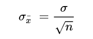
To calculate standard error, you simply divide the standard deviation of a given sample by the square root of the total number of items in the sample.

$$SE_{bar{x}} = frac{sigma}{sqrt{n}}$$

where, $SE_{bar{x}}$ is the standard error of the mean, $sigma$ is the standard deviation of the sample and n is the number of items in sample.

Do not confuse this with standard deviation. Because standard error of the sample statistic (like mean) is typically much smaller than the population standard deviation.

Notice few things here:

1. The Standard error depends on the number of items in the sample. As you increase the number of items in the sample, lower will be the standard error and more certain you will be about the estimates.
2. It uses statistics (standard deviation and number of items) computed from the sample itself, and not of the population. That is, you don’t need to know the population parameters beforehand to compute standard error. This makes it pretty convenient.
3. Standard error can also be used as an estimate of how representative a given sample is of a population. The smaller the value, more representative is the sample of the whole population.

Below is a computation for the standard error of the mean:

# Compute Standard Error
sample1 = [400, 420, 470, 510, 590]
se = stdev(sample1)/len(sample1)
print('Standard Error: ', round(se, 2))

Standard Error:  15.19

How to calculate standard error?

Problem Statement

A school aptitude test for 15 year old students studying in a particular territory’s curriculum, is designed to have a mean score of 80 units and a standard deviation of 10 units. A sample of 15 answer papers has a mean score of 85. Can we assume that these 15 scores come from the designated population?

Solution

Our task is to determine if this sample comes from the above mentioned population.

How to solve this?

We approach this problem by computing the standard error of the sample means and use it to compute the confidence interval between which the sample means are expected to fall.

If the given sample mean falls inside this interval, then its safe to assume that the sample comes from the given population.

Time to get into the math.

Using standard error to compute confidence interval

Standard error is often used to compute confidence intervals

We know, n = 15, x_bar = 85, σ = 10

$$SE_bar{x} = frac{sigma}{sqrt{n}} = frac{10}{sqrt{15}} = 2.581$$

From a property of normal distribution, we can say with 95% confidence level that the sample means are expected to lie within a confidence interval of plus or minus two standard errors of the sample statistic from the population parameter.

But where did ‘normal distribution’ come from? You may wonder how we can directly assume a normal distribution is followed in this case. Or rather shouldn’t we test if the sample follows a normal distribution first before computing the confidence intervals.

Well, that’s NOT required. Because, the Central Limit Theorem tells us that even if a population is not normally distributed, a collection of sample means from that population will infact follow a normal distribution. So, its a valid assumption.

Back to the problem, let’s compute the confidence intervals for 95% Confidence Level.

• Lower Limit : 80 - (2*2.581) = 74.838
• Upper Limit : 80 + (2*2.581) = 85.162

So, 95% of our 15 item sample means are expected to fall between 74.838 and 85.162.

Since the sample mean of 85.0 lies within the computed range, there is no reason to believe that the sample does not belong to the population.

Conclusion

Standard error is a commonly used term that we sometimes ignore to fully understand its significance. I hope the concept is clear and you can now relate how you can use standard error in appropriate situations.

Next topic: Confidence Interval

Errors are of various types and impact the research process in different ways. Here’s a deep exploration of the standard error, the types, implications, formula, and how to interpret the values

What is a Standard Error? 

The standard error is a statistical measure that accounts for the extent to which a sample distribution represents the population of interest using standard deviation. You can also think of it as the standard deviation of your sample in relation to your target population. 

The standard error allows you to compare two similar measures in your sample data and population. For example, the standard error of the mean measures how far the sample mean (average) of the data is likely to be from the true population mean—the same applies to other types of standard errors. 

Explore: Survey Errors To Avoid: Types, Sources, Examples, Mitigation

Why is Standard Error Important? 

First, the standard error of a sample accounts for statistical fluctuation.

Researchers depend on this statistical measure to know how much sampling fluctuation exists in their sample data. In other words, it shows the extent to which a statistical measure varies from sample to population. 

In addition, standard error serves as a measure of accuracy. Using standard error, a researcher can estimate the efficiency and consistency of a sample to know precisely how a sampling distribution represents a population. 

How Many Types of Standard Error Exist?

There are five types of standard error which are:

1. Standard error of the mean
2. Standard error of measurement
3. Standard error of the proportion
4. Standard error of estimate
5. Residual Standard Error

1. Standard Error of the Mean (SEM) 

The standard error of the mean accounts for the difference between the sample mean and the population mean. In other words, it quantifies how much variation is expected to be present in the sample mean that would be computed from every possible sample, of a given size, taken from the population. 

How to Find SEM (With Formula)

SEM = Standard Deviation ÷ √n 

Where; 

n = sample size 

Suppose that the standard deviation of observation is 15 with a sample size of 100. Using this formula, we can deduce the standard error of the mean as follows: 

SEM = 15 ÷ √100 

Standard Error of Mean in 1.5 

2. Standard Error of Measurement

The standard error of measurement accounts for the consistency of scores within individual subjects in a test or examination.

This means it measures the extent to which estimated test or examination scores are spread around a true score. 

A more formal way to look at it is through the 1985 lens of Aera, APA, and NCME. Here, they define a standard error as “the standard deviation of errors of measurement that is associated with the test scores for a specified group of test-takers….” 

Read: 7 Types of Data Measurement Scales in Research

How to Find Standard Error of Measurement

Where; 

rxx is the reliability of the test and is calculated as: 

Rxx = S2T / S2X

Where; 

S2T = variance of the true scores.

S2X = variance of the observed scores.

Suppose an organization has a reliability score of 0.4 and a standard deviation of 2.56. This means

SEm = 2.56 × √1–0.4 = 1.98 

3. Standard Error of the Estimate 

The standard error of the estimate measures the accuracy of predictions in sampling, research, and data collection. Specifically, it measures the distance that the observed values fall from the regression line which is the single line with the smallest overall distance from the line to the points. 

How to Find Standard Error of the Estimate

The formula for standard error of the estimate is as follows: 

Where;

σest is the standard error of the estimate;

Y is an actual score;

Y’ is a predicted score, and; 

N is the number of pairs of scores. 

The numerator is the sum of squared differences between the actual scores and the predicted scores.

4. Standard Error of Proportion 

The standard of error of proportion in an observation is the difference between the sample proportion and the population proportion of your target audience. In more technical terms, this variable is the spread of the sample proportion about the population proportion. 

How to Find Standard Error of the Proportion 

The formula for calculating the standard error of the proportion is as follows: 

Where; 

P (hat) is equal to x ÷ n (with number of success x and the total number of observations of n) 

5. Residual Standard Error 

Residual standard error accounts for how well a linear regression model fits the observation in a systematic investigation. A linear regression model is simply a linear equation representing the relationship between two variables, and it helps you to predict similar variables. 

How to Calculate Residual Standard Error 

The formula for residual standard error is as follows: 

Residual standard error = √Σ(y – ŷ)2/df 

where:

y: The observed value

ŷ: The predicted value

df: The degrees of freedom, calculated as the total number of observations – total number of model parameters.

As you interpret your data, you should note that the smaller the residual standard error, the better a regression model fits a dataset, and vice versa. 

How Do You Calculate Standard Error? 

The formula for calculating standard error is as follows: 

Where

σ – Standard deviation

n – Sample size, i.e., the number of observations in the sample 

Here’s how this works in real-time. 

Suppose the standard deviation of a sample is 1.5 with 4 as the sample size. This means:

Standard Error = 1.5 ÷ √4 

That is; 1.5 ÷2 = 0.75 

Alternatively, you can use a standard error calculator to speed up the process for larger data sets. 

How to Interpret Standard Error Values

As stated earlier, researchers use the standard error to measure the reliability of observation. This means it allows you to compare how far a particular variable in the sample data is from the population of interest. 

Calculating standard error is just one piece of the puzzle; you need to know how to interpret your data correctly and draw useful insights for your research. Generally, a small standard error is an indication that the sample mean is a more accurate reflection of the actual population mean, while a large standard error means the opposite. 

Standard Error Example

Suppose you need to find the standard error of the mean of a data set using the following information: 

Standard Deviation: 1.5 

n = 13 

Standard Error of the Mean =  Standard Deviation ÷ √n 

1.5 ÷ √13 = 0.42

How Should You Report the Standard Error?

After calculating the standard error of your observation, the next thing you should do is present this data as part of the numerous variables affecting your observation. Typically, researchers report the standard error alongside the mean or in a confidence interval to communicate the uncertainty around the mean. 

Applications of Standard Error

The most common application of standard error are in statistics and economics. In statistics, standard error allows researchers to determine the confidence interval of their data sets, and in some cases, the margin of error. Researchers also use standard error in hypothesis testing and regression analysis. 

FAQs About Standard Error

• What Is the Difference Between Standard Deviation and Standard Error of the Mean? 

The major difference between standard deviation and standard error of the mean is how they account for the differences between the sample data and the population of interest. 

Researchers use standard deviation to measure the variability or dispersion of a data set to its mean. On the other hand, the standard error of the mean accounts for the difference between the mean of the data sample and that of the target population. 

Something else to note here is that the standard error of a sample is always smaller than the corresponding standard deviation. 

• What Is The Symbol for Standard Error?

During calculation, the standard error is represented as σx̅. 

• Is Standard Error the Same as Margin of Error?

No. Margin of Error and standard error are not the same. Researchers use the standard error to measure the preciseness of an estimate of a population, meanwhile margin of error accounts for the degree of error in results received from random sampling surveys.

The standard error is calculated as s / √n where; 

s: Sample standard deviation

n: Sample size

On the other hand, margin of error = z*(s/√n) where:

z: Z value that corresponds to a given confidence level

s: Sample standard deviation

n: Sample size

Published on
December 11, 2020
by

Pritha Bhandari.

Revised on
December 19, 2022.

The standard error of the mean, or simply standard error, indicates how different the population mean is likely to be from a sample mean. It tells you how much the sample mean would vary if you were to repeat a study using new samples from within a single population.

The standard error of the mean (SE or SEM) is the most commonly reported type of standard error. But you can also find the standard error for other statistics, like medians or proportions. The standard error is a common measure of sampling error—the difference between a population parameter and a sample statistic.

Table of contents

1. Why standard error matters
2. Standard error vs standard deviation
3. Standard error formula
4. How should you report the standard error?
5. Other standard errors
6. Frequently asked questions about standard error

Why standard error matters

In statistics, data from samples is used to understand larger populations. Standard error matters because it helps you estimate how well your sample data represents the whole population.

With probability sampling, where elements of a sample are randomly selected, you can collect data that is likely to be representative of the population. However, even with probability samples, some sampling error will remain. That’s because a sample will never perfectly match the population it comes from in terms of measures like means and standard deviations.

By calculating standard error, you can estimate how representative your sample is of your population and make valid conclusions.

A high standard error shows that sample means are widely spread around the population mean—your sample may not closely represent your population. A low standard error shows that sample means are closely distributed around the population mean—your sample is representative of your population.

You can decrease standard error by increasing sample size. Using a large, random sample is the best way to minimize sampling bias.

Standard error vs standard deviation

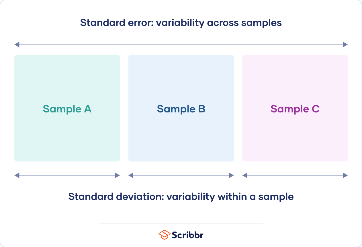
Standard error and standard deviation are both measures of variability:

• The standard deviation describes variability within a single sample.
• The standard error estimates the variability across multiple samples of a population.

The standard deviation is a descriptive statistic that can be calculated from sample data. In contrast, the standard error is an inferential statistic that can only be estimated (unless the real population parameter is known).

In a random sample of 200 students, the mean math SAT score is 550. In this case, the sample is the 200 students, while the population is all test takers in the region.

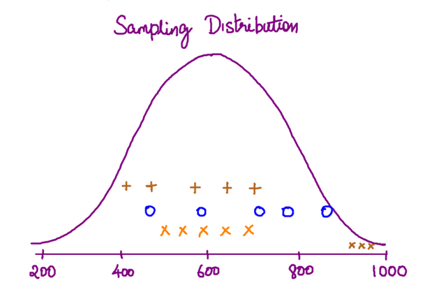
The standard deviation of the math scores is 180. This number reflects on average how much each score differs from the sample mean score of 550.

The standard error of the math scores, on the other hand, tells you how much the sample mean score of 550 differs from other sample mean scores, in samples of equal size, in the population of all test takers in the region.

What can proofreading do for your paper?

Scribbr editors not only correct grammar and spelling mistakes, but also strengthen your writing by making sure your paper is free of vague language, redundant words, and awkward phrasing.

See editing example

Standard error formula

The standard error of the mean is calculated using the standard deviation and the sample size.

From the formula, you’ll see that the sample size is inversely proportional to the standard error. This means that the larger the sample, the smaller the standard error, because the sample statistic will be closer to approaching the population parameter.

Different formulas are used depending on whether the population standard deviation is known. These formulas work for samples with more than 20 elements (n > 20).

When population parameters are known

When the population standard deviation is known, you can use it in the below formula to calculate standard error precisely.

Formula	Explanation
	is standard error is population standard deviation is the number of elements in the sample

When population parameters are unknown

When the population standard deviation is unknown, you can use the below formula to only estimate standard error. This formula takes the sample standard deviation as a point estimate for the population standard deviation.

Formula	Explanation
	is standard error is sample standard deviation is the number of elements in the sample

To estimate the standard error for math SAT scores, you follow two steps.

First, find the square root of your sample size (n).

Formula	Calculation

Next, divide the sample standard deviation by the number you found in step one.

Formula	Calculation

The standard error of math SAT scores is 12.8.

How should you report the standard error?

You can report the standard error alongside the mean or in a confidence interval to communicate the uncertainty around the mean.

The mean math SAT score of a random sample of test takers is 550 ± 12.8 (SE).

The best way to report the standard error is in a confidence interval because readers won’t have to do any additional math to come up with a meaningful interval.

A confidence interval is a range of values where an unknown population parameter is expected to lie most of the time, if you were to repeat your study with new random samples.

With a 95% confidence level, 95% of all sample means will be expected to lie within a confidence interval of ± 1.96 standard errors of the sample mean.

Based on random sampling, the true population parameter is also estimated to lie within this range with 95% confidence.

You construct a 95% confidence interval (CI) to estimate the population mean math SAT score.

For a normally distributed characteristic, like SAT scores, 95% of all sample means fall within roughly 4 standard errors of the sample mean.

Confidence interval formula
CI = x̄ ± (1.96 × SE) x̄ = sample mean = 550 SE = standard error = 12.8
Lower limit	Upper limit
x̄ − (1.96 × SE) 550 − (1.96 × 12.8) = 525	x̄ + (1.96 × SE) 550 + (1.96 × 12.8) = 575

With random sampling, a 95% CI [525 575] tells you that there is a 0.95 probability that the population mean math SAT score is between 525 and 575.

Other standard errors

Aside from the standard error of the mean (and other statistics), there are two other standard errors you might come across: the standard error of the estimate and the standard error of measurement.

The standard error of the estimate is related to regression analysis. This reflects the variability around the estimated regression line and the accuracy of the regression model. Using the standard error of the estimate, you can construct a confidence interval for the true regression coefficient.

The standard error of measurement is about the reliability of a measure. It indicates how variable the measurement error of a test is, and it’s often reported in standardized testing. The standard error of measurement can be used to create a confidence interval for the true score of an element or an individual.

Frequently asked questions about standard error

What is standard error?

The standard error of the mean, or simply standard error, indicates how different the population mean is likely to be from a sample mean. It tells you how much the sample mean would vary if you were to repeat a study using new samples from within a single population.

Cite this Scribbr article

If you want to cite this source, you can copy and paste the citation or click the “Cite this Scribbr article” button to automatically add the citation to our free Citation Generator.

Bhandari, P.
(2022, December 19). What Is Standard Error? | How to Calculate (Guide with Examples). Scribbr.
Retrieved February 9, 2023,
from https://www.scribbr.com/statistics/standard-error/

Is this article helpful?

You have already voted. Thanks
Your vote is saved
Processing your vote…

Стандартная ошибка ( SE ) ^[1] статистического показателя ( обычно оценка параметра ) — это стандартное отклонение его выборочного распределения ^[2] или оценка этого стандартного отклонения. Если статистика является выборочным средним, она называется стандартной ошибкой среднего ( SEM ). ^[1]

Выборочное распределение среднего создается путем повторной выборки из одной и той же совокупности и регистрации полученных выборочных средних. Это формирует распределение различных средних значений, и это распределение имеет свое собственное среднее значение и дисперсию . Математически дисперсия полученного выборочного распределения равна дисперсии генеральной совокупности, деленной на размер выборки. Это связано с тем, что по мере увеличения размера выборки средние значения выборки теснее группируются вокруг среднего значения генеральной совокупности.

Таким образом, соотношение между стандартной ошибкой среднего и стандартным отклонением таково, что для данного размера выборки стандартная ошибка среднего равна стандартному отклонению, деленному на квадратный корень из размера выборки. ^[1] Другими словами, стандартная ошибка среднего является мерой дисперсии выборочных средних значений относительно среднего значения генеральной совокупности.

В регрессионном анализе термин «стандартная ошибка» относится либо к квадратному корню из приведенной статистики хи-квадрат , либо к стандартной ошибке для конкретного коэффициента регрессии (как используется, скажем, в доверительных интервалах ).

Стандартная ошибка среднего

Точное значение

Если статистически независимая выборканаблюденияберется из статистической совокупности со стандартным отклонением, то среднее значение, рассчитанное по выборкебудет иметь соответствующую стандартную ошибку в среднем дано: ^[1]

.

Практически это говорит нам о том, что при попытке оценить значение среднего значения совокупности из-за фактора, уменьшение ошибки оценки в два раза требует получения в четыре раза большего количества наблюдений в выборке; уменьшение его в десять раз требует в сто раз больше наблюдений.

Оценить

Стандартное отклонениео выборке населения редко известно. Поэтому стандартная ошибка среднего обычно оценивается путем заменысо стандартным отклонением выборки вместо:

.

Поскольку это только оценка истинной «стандартной ошибки», здесь часто встречаются другие обозначения, такие как:

 или попеременно  .

Обычный источник путаницы возникает, когда не удается четко разграничить стандартное отклонение совокупности (), стандартное отклонение выборки (), стандартное отклонение самого среднего (, что является стандартной ошибкой), и оценка стандартного отклонения среднего (, которая является наиболее часто вычисляемой величиной, а также часто в просторечии называется стандартной ошибкой ).

Точность оценки

Когда размер выборки мал, использование стандартного отклонения выборки вместо истинного стандартного отклонения генеральной совокупности приведет к систематической недооценке стандартного отклонения генеральной совокупности и, следовательно, стандартной ошибки. При n = 2 недооценка составляет около 25%, а при n = 6 недооценка составляет всего 5%. Гурланд и Трипати (1971) предлагают поправку и уравнение для этого эффекта. ^[3] Sokal and Rohlf (1981) дают уравнение поправочного коэффициента для небольших выборок n < 20. ^[4] Для дальнейшего обсуждения
см . объективную оценку стандартного отклонения .

Происхождение

Стандартная ошибка среднего может быть получена из дисперсии суммы независимых случайных величин ^[5] с учетом определения дисперсии и некоторых ее простых свойств . Еслиявляютсянезависимые наблюдения за популяцией со средними стандартное отклонение, то мы можем определить общее

который в силу формулы Бьенеме будет иметь дисперсию

Среднее значение этих измеренийпросто дается

.

Тогда дисперсия среднего

Стандартная ошибка – это, по определению, стандартное отклонениекоторый представляет собой просто квадратный корень из дисперсии:

.

Для коррелированных случайных величин выборочная дисперсия должна быть рассчитана в соответствии с центральной предельной теоремой цепи Маркова .

Независимые и одинаково распределенные случайные величины со случайным размером выборки

Бывают случаи, когда выборку берут, не зная заранее, сколько наблюдений будет приемлемо по тому или иному критерию. В таких случаях размер выборкиявляется случайной величиной, вариация которой добавляется к вариациитакой, что

^[6]

Еслиимеет распределение Пуассона , тос оценщиком. Следовательно, оценкастановится, приводя следующую формулу для стандартной ошибки:

(поскольку стандартное отклонение представляет собой квадратный корень из дисперсии)

Аппроксимация Стьюдента, когда значение σ неизвестно

Во многих практических приложениях истинное значение σ неизвестно. В результате нам нужно использовать распределение, учитывающее этот разброс возможных σ’с. Когда известно, что истинное базовое распределение является гауссовым, хотя и с неизвестным σ, то результирующее оценочное распределение соответствует t-распределению Стьюдента. Стандартная ошибка представляет собой стандартное отклонение t-распределения Стьюдента. T-распределения немного отличаются от гауссовых и меняются в зависимости от размера выборки. Небольшие выборки с несколько большей вероятностью недооценивают стандартное отклонение совокупности и имеют среднее значение, которое отличается от истинного среднего значения совокупности, а t-распределение Стьюдента объясняет вероятность этих событий с несколько более тяжелыми хвостами по сравнению с гауссовским. Для оценки стандартной ошибки t-распределения Стьюдента достаточно использовать выборочное стандартное отклонение «s» вместо σ , и мы могли бы использовать это значение для расчета доверительных интервалов.

Примечание. Распределение вероятностей Стьюдента хорошо аппроксимируется распределением Гаусса, когда размер выборки превышает 100. Для таких выборок можно использовать последнее распределение, которое намного проще.

Предположения и использование

Пример того, какиспользуется для того, чтобы сделать доверительные интервалы неизвестной генеральной совокупности средними. Если распределение выборки имеет нормальное распределение , то выборочное среднее, стандартная ошибка и квантили нормального распределения могут использоваться для расчета доверительных интервалов для истинного среднего значения генеральной совокупности. Следующие выражения можно использовать для расчета верхнего и нижнего 95%-го доверительного интервала, гдеравно выборочному среднему,равно стандартной ошибке выборочного среднего, а 1,96 — это приблизительное значение точки 97,5 процентиля нормального распределения :

Верхний предел 95%а также

Нижний предел 95%

В частности, стандартная ошибка выборочной статистики (такой как выборочное среднее ) — это фактическое или оценочное стандартное отклонение выборочного среднего в процессе, с помощью которого оно было получено. Другими словами, это фактическое или оценочное стандартное отклонение выборочного распределения выборочной статистики. Обозначение стандартной ошибки может быть любым из SE, SEM (стандартная ошибка измерения или среднего значения ) или _SE .

Стандартные ошибки обеспечивают простые меры неопределенности значения и часто используются, потому что:

• во многих случаях, если известна стандартная ошибка нескольких отдельных величин, то можно легко вычислить стандартную ошибку некоторой функции этих величин;
• когда известно распределение вероятностей значения, его можно использовать для расчета точного доверительного интервала ;
• когда распределение вероятностей неизвестно, для расчета консервативного доверительного интервала можно использовать неравенства Чебышева или Высочанского–Петунина ; а также
• поскольку размер выборки стремится к бесконечности, центральная предельная теорема гарантирует, что выборочное распределение среднего является асимптотически нормальным .

Стандартная ошибка среднего по сравнению со стандартным отклонением

В научно-технической литературе экспериментальные данные часто обобщаются либо с использованием среднего значения и стандартного отклонения выборочных данных, либо среднего значения со стандартной ошибкой. Это часто приводит к путанице в отношении их взаимозаменяемости. Однако среднее значение и стандартное отклонение являются описательной статистикой , тогда как стандартная ошибка среднего значения описывает процесс случайной выборки. Стандартное отклонение выборочных данных — это описание вариаций в измерениях, а стандартная ошибка среднего — вероятностное утверждение о том, как размер выборки обеспечит лучшую оценку среднего значения генеральной совокупности в свете центрального предела. теорема. ^[7]

Проще говоря, стандартная ошибка среднего значения выборки — это оценка того, насколько вероятно среднее значение выборки будет отличаться от среднего значения генеральной совокупности, тогда как стандартное отклонение выборки — это степень, в которой отдельные лица в выборке отличаются от среднего значения выборки. ^[8] Если стандартное отклонение совокупности конечно, стандартная ошибка среднего значения выборки будет стремиться к нулю с увеличением размера выборки, потому что оценка среднего значения совокупности будет улучшаться, в то время как стандартное отклонение выборки будет приближаться к стандартное отклонение генеральной совокупности по мере увеличения размера выборки.

Расширения

Коррекция конечной популяции (FPC)

Приведенная выше формула для стандартной ошибки предполагает, что размер выборки намного меньше, чем размер совокупности, так что совокупность можно считать фактически бесконечной по размеру. Обычно это происходит даже с конечными популяциями, потому что большую часть времени люди в первую очередь заинтересованы в управлении процессами, которые создали существующую конечную популяцию; это называется аналитическим исследованием вслед за У. Эдвардсом Демингом . Если люди заинтересованы в управлении существующей конечной популяцией, которая не изменится с течением времени, необходимо сделать поправку на размер популяции; это называется перечислительным исследованием .

Когда доля выборки (часто называемая f ) велика (приблизительно 5% или более) в перечислительном исследовании , оценка стандартной ошибки должна быть скорректирована путем умножения на «поправку на конечную совокупность» (она же: fpc ): ^[9]
[10]

что для больших N :

для учета дополнительной точности, полученной за счет выборки, близкой к большему проценту населения. Эффект FPC заключается в том, что ошибка становится равной нулю ,
когда размер выборки n равен размеру совокупности N.

Это происходит в методологии обследования при выборке без возмещения . Если выборка с заменой, то ФПК не играет роли.

Поправка на корреляцию в выборке

Если значения измеренной величины A не являются статистически независимыми, а были получены из известных местоположений в пространстве параметров  x , несмещенная оценка истинной стандартной ошибки среднего (фактически поправка на часть стандартного отклонения) может быть получена путем умножения рассчитанная стандартная ошибка выборки по фактору  f :

где коэффициент смещения выборки ρ — это широко используемая оценка Прайса – Винстена коэффициента автокорреляции (величина от -1 до +1) для всех пар точек выборки. Эта приблизительная формула предназначена для средних и больших размеров выборки; ссылка дает точные формулы для любого размера выборки и может применяться к сильно автокоррелированным временным рядам, таким как котировки акций Уолл-стрит. Более того, эта формула работает как для положительных, так и для отрицательных ρ. ^[11] См. также несмещенную оценку стандартного отклонения для дальнейшего обсуждения.

Смотрите также

• Иллюстрация центральной предельной теоремы
• Погрешность
• Вероятная ошибка
• Стандартная ошибка взвешенного среднего
• Выборочное среднее и выборочная ковариация
• Стандартная ошибка медианы
• Дисперсия

Ссылки

Об этой статье

Была ли эта статья полезной?