A t-test is any statistical hypothesis test in which the test statistic follows a Student’s t-distribution under the null hypothesis. It is most commonly applied when the test statistic would follow a normal distribution if the value of a scaling term in the test statistic were known (typically, the scaling term is unknown and therefore a nuisance parameter). When the scaling term is estimated based on the data, the test statistic—under certain conditions—follows a Student’s t distribution. The t-test’s most common application is to test whether the means of two populations are different.
History[edit]

The term «t-statistic» is abbreviated from «hypothesis test statistic».[1] In statistics, the t-distribution was first derived as a posterior distribution in 1876 by Helmert[2][3][4] and Lüroth.[5][6][7] The t-distribution also appeared in a more general form as Pearson Type IV distribution in Karl Pearson’s 1895 paper.[8] However, the T-Distribution, also known as Student’s t-distribution, gets its name from William Sealy Gosset who first published it in English in 1908 in the scientific journal Biometrika using the pseudonym «Student»[9][10] because his employer preferred staff to use pen names when publishing scientific papers.[11] Gosset worked at the Guinness Brewery in Dublin, Ireland, and was interested in the problems of small samples – for example, the chemical properties of barley with small sample sizes. Hence a second version of the etymology of the term Student is that Guinness did not want their competitors to know that they were using the t-test to determine the quality of raw material (see Student’s t-distribution for a detailed history of this pseudonym, which is not to be confused with the literal term student). Although it was William Gosset after whom the term «Student» is penned, it was actually through the work of Ronald Fisher that the distribution became well known as «Student’s distribution»[12] and «Student’s t-test».
Gosset had been hired owing to Claude Guinness’s policy of recruiting the best graduates from Oxford and Cambridge to apply biochemistry and statistics to Guinness’s industrial processes.[13] Gosset devised the t-test as an economical way to monitor the quality of stout. The t-test work was submitted to and accepted in the journal Biometrika and published in 1908.[14]
Guinness had a policy of allowing technical staff leave for study (so-called «study leave»), which Gosset used during the first two terms of the 1906–1907 academic year in Professor Karl Pearson’s Biometric Laboratory at University College London.[15] Gosset’s identity was then known to fellow statisticians and to editor-in-chief Karl Pearson.[16]
Uses[edit]
The most frequently used t-tests are one-sample and two-sample tests:
- A one-sample location test of whether the mean of a population has a value specified in a null hypothesis.
- A two-sample location test of the null hypothesis such that the means of two populations are equal. All such tests are usually called Student’s t-tests, though strictly speaking that name should only be used if the variances of the two populations are also assumed to be equal; the form of the test used when this assumption is dropped is sometimes called Welch’s t-test. These tests are often referred to as unpaired or independent samples t-tests, as they are typically applied when the statistical units underlying the two samples being compared are non-overlapping.[17]
Assumptions[edit]
[dubious – discuss]
Most test statistics have the form t = Z/s, where Z and s are functions of the data.
Z may be sensitive to the alternative hypothesis (i.e., its magnitude tends to be larger when the alternative hypothesis is true), whereas s is a scaling parameter that allows the distribution of t to be determined.
As an example, in the one-sample t-test

where X is the sample mean from a sample X1, X2, …, Xn, of size n, s is the standard error of the mean,  is the estimate of the standard deviation of the population, and μ is the population mean.
The assumptions underlying a t-test in the simplest form above are that:
- X follows a normal distribution with mean μ and variance σ2/n
- s2(n − 1)/σ2 follows a χ2 distribution with n − 1 degrees of freedom. This assumption is met when the observations used for estimating s2 come from a normal distribution (and i.i.d for each group).
- Z and s are independent.
In the t-test comparing the means of two independent samples, the following assumptions should be met:
- The means of the two populations being compared should follow normal distributions. Under weak assumptions, this follows in large samples from the central limit theorem, even when the distribution of observations in each group is non-normal.[18]
- If using Student’s original definition of the t-test, the two populations being compared should have the same variance (testable using F-test, Levene’s test, Bartlett’s test, or the Brown–Forsythe test; or assessable graphically using a Q–Q plot). If the sample sizes in the two groups being compared are equal, Student’s original t-test is highly robust to the presence of unequal variances.[19] Welch’s t-test is insensitive to equality of the variances regardless of whether the sample sizes are similar.
- The data used to carry out the test should either be sampled independently from the two populations being compared or be fully paired. This is in general not testable from the data, but if the data are known to be dependent (e.g. paired by test design), a dependent test has to be applied. For partially paired data, the classical independent t-tests may give invalid results as the test statistic might not follow a t distribution, while the dependent t-test is sub-optimal as it discards the unpaired data.[20]
Most two-sample t-tests are robust to all but large deviations from the assumptions.[21]
For exactness, the t-test and Z-test require normality of the sample means, and the t-test additionally requires that the sample variance follows a scaled χ2 distribution, and that the sample mean and sample variance be statistically independent. Normality of the individual data values is not required if these conditions are met. By the central limit theorem, sample means of moderately large samples are often well-approximated by a normal distribution even if the data are not normally distributed. For non-normal data, the distribution of the sample variance may deviate substantially from a χ2 distribution.
However, if the sample size is large, Slutsky’s theorem implies that the distribution of the sample variance has little effect on the distribution of the test statistic. That is as sample size  increases:
Unpaired and paired two-sample t-tests[edit]
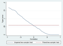
Type I error of unpaired and paired two-sample t-tests as a function of the correlation. The simulated random numbers originate from a bivariate normal distribution with a variance of 1. The significance level is 5% and the number of cases is 60.

Power of unpaired and paired two-sample t-tests as a function of the correlation. The simulated random numbers originate from a bivariate normal distribution with a variance of 1 and a deviation of the expected value of 0.4. The significance level is 5% and the number of cases is 60.
Two-sample t-tests for a difference in means involve independent samples (unpaired samples) or paired samples. Paired t-tests are a form of blocking, and have greater power (probability of avoiding a type II error, also known as a false negative) than unpaired tests when the paired units are similar with respect to «noise factors» that are independent of membership in the two groups being compared.[22] In a different context, paired t-tests can be used to reduce the effects of confounding factors in an observational study.
Independent (unpaired) samples[edit]
The independent samples t-test is used when two separate sets of independent and identically distributed samples are obtained, and one variable from each of the two populations is compared. For example, suppose we are evaluating the effect of a medical treatment, and we enroll 100 subjects into our study, then randomly assign 50 subjects to the treatment group and 50 subjects to the control group. In this case, we have two independent samples and would use the unpaired form of the t-test.
Paired samples[edit]
Paired samples t-tests typically consist of a sample of matched pairs of similar units, or one group of units that has been tested twice (a «repeated measures» t-test).
A typical example of the repeated measures t-test would be where subjects are tested prior to a treatment, say for high blood pressure, and the same subjects are tested again after treatment with a blood-pressure-lowering medication. By comparing the same patient’s numbers before and after treatment, we are effectively using each patient as their own control. That way the correct rejection of the null hypothesis (here: of no difference made by the treatment) can become much more likely, with statistical power increasing simply because the random interpatient variation has now been eliminated. However, an increase of statistical power comes at a price: more tests are required, each subject having to be tested twice. Because half of the sample now depends on the other half, the paired version of Student’s t-test has only n/2 − 1 degrees of freedom (with n being the total number of observations). Pairs become individual test units, and the sample has to be doubled to achieve the same number of degrees of freedom. Normally, there are n − 1 degrees of freedom (with n being the total number of observations).[23]
A paired samples t-test based on a «matched-pairs sample» results from an unpaired sample that is subsequently used to form a paired sample, by using additional variables that were measured along with the variable of interest.[24] The matching is carried out by identifying pairs of values consisting of one observation from each of the two samples, where the pair is similar in terms of other measured variables. This approach is sometimes used in observational studies to reduce or eliminate the effects of confounding factors.
Paired samples t-tests are often referred to as «dependent samples t-tests».
Calculations[edit]
Explicit expressions that can be used to carry out various t-tests are given below. In each case, the formula for a test statistic that either exactly follows or closely approximates a t-distribution under the null hypothesis is given. Also, the appropriate degrees of freedom are given in each case. Each of these statistics can be used to carry out either a one-tailed or two-tailed test.
Once the t value and degrees of freedom are determined, a p-value can be found using a table of values from Student’s t-distribution. If the calculated p-value is below the threshold chosen for statistical significance (usually the 0.10, the 0.05, or 0.01 level), then the null hypothesis is rejected in favor of the alternative hypothesis.
One-sample t-test[edit]
In testing the null hypothesis that the population mean is equal to a specified value μ0, one uses the statistic

where  is the sample mean, s is the sample standard deviation and n is the sample size. The degrees of freedom used in this test are n − 1.
Although the parent population does not need to be normally distributed, the distribution of the population of sample means is assumed to be normal.
By the central limit theorem, if the observations are independent and the second moment exists, then  will be approximately normal N(0;1).
Slope of a regression line[edit]
Suppose one is fitting the model

where x is known, α and β are unknown, ε is a normally distributed random variable with mean 0 and unknown variance σ2, and Y is the outcome of interest. We want to test the null hypothesis that the slope β is equal to some specified value β0 (often taken to be 0, in which case the null hypothesis is that x and y are uncorrelated).
Let

Then

has a t-distribution with n − 2 degrees of freedom if the null hypothesis is true. The standard error of the slope coefficient:

can be written in terms of the residuals. Let

Then tscore is given by:

Another way to determine the tscore is:

where r is the Pearson correlation coefficient.
The tscore, intercept can be determined from the tscore, slope:

where sx2 is the sample variance.
Independent two-sample t-test[edit]
Equal sample sizes and variance[edit]
Given two groups (1, 2), this test is only applicable when:
- the two sample sizes are equal;
- it can be assumed that the two distributions have the same variance;
Violations of these assumptions are discussed below.
The t statistic to test whether the means are different can be calculated as follows:

where

Here sp is the pooled standard deviation for n = n1 = n2 and s 2
X1 and s 2
X2 are the unbiased estimators of the population variance. The denominator of t is the standard error of the difference between two means.
For significance testing, the degrees of freedom for this test is 2n − 2 where n is sample size.
Equal or unequal sample sizes, similar variances (1/2 < sX1/sX2 < 2)[edit]
This test is used only when it can be assumed that the two distributions have the same variance. (When this assumption is violated, see below.)
The previous formulae are a special case of the formulae below, one recovers them when both samples are equal in size: n = n1 = n2.
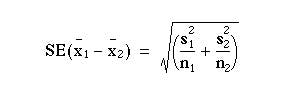
The t statistic to test whether the means are different can be calculated as follows:

where

is the pooled standard deviation of the two samples: it is defined in this way so that its square is an unbiased estimator of the common variance whether or not the population means are the same. In these formulae, ni − 1 is the number of degrees of freedom for each group, and the total sample size minus two (that is, n1 + n2 − 2) is the total number of degrees of freedom, which is used in significance testing.
Equal or unequal sample sizes, unequal variances (sX1 > 2sX2 or sX2 > 2sX1)[edit]
This test, also known as Welch’s t-test, is used only when the two population variances are not assumed to be equal (the two sample sizes may or may not be equal) and hence must be estimated separately. The t statistic to test whether the population means are different is calculated as:

where

Here si2 is the unbiased estimator of the variance of each of the two samples with ni = number of participants in group i (i = 1 or 2). In this case

is not a pooled variance. For use in significance testing, the distribution of the test statistic is approximated as an ordinary Student’s t-distribution with the degrees of freedom calculated using

This is known as the Welch–Satterthwaite equation. The true distribution of the test statistic actually depends (slightly) on the two unknown population variances (see Behrens–Fisher problem).
Exact method for unequal variances and sample sizes[edit]
The test[25] deals with the famous Behrens–Fisher problem, i.e., comparing the difference between the means of two normally distributed populations when the variances of the two populations are not assumed to be equal, based on two independent samples.
The test is developed as an exact test that allows for unequal sample sizes and unequal variances of two populations. The exact property still holds even with small extremely small and unbalanced sample sizes (e.g.  ).
).
The statistic to test whether the means are different can be calculated as follows:
Let ![{displaystyle X=[X_{1},X_{2},ldots ,X_{m}]^{T}}](https://wikimedia.org/api/rest_v1/media/math/render/svg/a0f37f25b326e4b6229a7f0be5283ace07d1a97f) and
and ![{displaystyle Y=[Y_{1},Y_{2},ldots ,Y_{n}]^{T}}](https://wikimedia.org/api/rest_v1/media/math/render/svg/a81b49d1f74f1a3c22759407966c63524eac1d2e) be the i.i.d. sample vectors (
be the i.i.d. sample vectors ( ) from
  and
and  separately.
Let  be an
be an  orthogonal matrix whose elements of the first row are all
  , similarly, let
  be the first n rows of an
  orthogonal matrix (whose elements of the first row are all
  ).
).
Then  is an n-dimensional normal random vector.

From the above distribution we see that


Dependent t-test for paired samples[edit]
This test is used when the samples are dependent; that is, when there is only one sample that has been tested twice (repeated measures) or when there are two samples that have been matched or «paired». This is an example of a paired difference test. The t statistic is calculated as

where  and
and  are the average and standard deviation of the differences between all pairs. The pairs are e.g. either one person’s pre-test and post-test scores or between-pairs of persons matched into meaningful groups (for instance drawn from the same family or age group: see table). The constant μ0 is zero if we want to test whether the average of the difference is significantly different. The degree of freedom used is n − 1, where n represents the number of pairs.
-
Example of repeated measures
Number Name Test 1 Test 2 1 Mike 35% 67% 2 Melanie 50% 46% 3 Melissa 90% 86% 4 Mitchell 78% 91%
-
Example of matched pairs
Pair Name Age Test 1 John 35 250 1 Jane 36 340 2 Jimmy 22 460 2 Jessy 21 200
Worked examples[edit]
Let A1 denote a set obtained by drawing a random sample of six measurements:

and let A2 denote a second set obtained similarly:

These could be, for example, the weights of screws that were chosen out of a bucket.
We will carry out tests of the null hypothesis that the means of the populations from which the two samples were taken are equal.
The difference between the two sample means, each denoted by Xi, which appears in the numerator for all the two-sample testing approaches discussed above, is

The sample standard deviations for the two samples are approximately 0.05 and 0.11, respectively. For such small samples, a test of equality between the two population variances would not be very powerful. Since the sample sizes are equal, the two forms of the two-sample t-test will perform similarly in this example.
Unequal variances[edit]
If the approach for unequal variances (discussed above) is followed, the results are

and the degrees of freedom

The test statistic is approximately 1.959, which gives a two-tailed test p-value of 0.09077.
Equal variances[edit]
If the approach for equal variances (discussed above) is followed, the results are

and the degrees of freedom

The test statistic is approximately equal to 1.959, which gives a two-tailed p-value of 0.07857.
[edit]
Alternatives to the t-test for location problems[edit]
The t-test provides an exact test for the equality of the means of two i.i.d. normal populations with unknown, but equal, variances. (Welch’s t-test is a nearly exact test for the case where the data are normal but the variances may differ.) For moderately large samples and a one tailed test, the t-test is relatively robust to moderate violations of the normality assumption.[26] In large enough samples, the t-test asymptotically approaches the z-test, and becomes robust even to large deviations from normality.[18]
If the data are substantially non-normal and the sample size is small, the t-test can give misleading results. See Location test for Gaussian scale mixture distributions for some theory related to one particular family of non-normal distributions.
When the normality assumption does not hold, a non-parametric alternative to the t-test may have better statistical power. However, when data are non-normal with differing variances between groups, a t-test may have better type-1 error control than some non-parametric alternatives.[27] Furthermore, non-parametric methods, such as the Mann-Whitney U test discussed below, typically do not test for a difference of means, so should be used carefully if a difference of means is of primary scientific interest.[18] For example, Mann-Whitney U test will keep the type 1 error at the desired level alpha if both groups have the same distribution. It will also have power in detecting an alternative by which group B has the same distribution as A but after some shift by a constant (in which case there would indeed be a difference in the means of the two groups). However, there could be cases where group A and B will have different distributions but with the same means (such as two distributions, one with positive skewness and the other with a negative one, but shifted so to have the same means). In such cases, MW could have more than alpha level power in rejecting the Null hypothesis but attributing the interpretation of difference in means to such a result would be incorrect.
In the presence of an outlier, the t-test is not robust. For example, for two independent samples when the data distributions are asymmetric (that is, the distributions are skewed) or the distributions have large tails, then the Wilcoxon rank-sum test (also known as the Mann–Whitney U test) can have three to four times higher power than the t-test.[26][28][29] The nonparametric counterpart to the paired samples t-test is the Wilcoxon signed-rank test for paired samples. For a discussion on choosing between the t-test and nonparametric alternatives, see Lumley, et al. (2002).[18]
One-way analysis of variance (ANOVA) generalizes the two-sample t-test when the data belong to more than two groups.
A design which includes both paired observations and independent observations[edit]
When both paired observations and independent observations are present in the two sample design, assuming data are missing completely at random (MCAR), the paired observations or independent observations may be discarded in order to proceed with the standard tests above. Alternatively making use of all of the available data, assuming normality and MCAR, the generalized partially overlapping samples t-test could be used.[30]
Multivariate testing[edit]
A generalization of Student’s t statistic, called Hotelling’s t-squared statistic, allows for the testing of hypotheses on multiple (often correlated) measures within the same sample. For instance, a researcher might submit a number of subjects to a personality test consisting of multiple personality scales (e.g. the Minnesota Multiphasic Personality Inventory). Because measures of this type are usually positively correlated, it is not advisable to conduct separate univariate t-tests to test hypotheses, as these would neglect the covariance among measures and inflate the chance of falsely rejecting at least one hypothesis (Type I error). In this case a single multivariate test is preferable for hypothesis testing. Fisher’s Method for combining multiple tests with alpha reduced for positive correlation among tests is one. Another is Hotelling’s T2 statistic follows a T2 distribution. However, in practice the distribution is rarely used, since tabulated values for T2 are hard to find. Usually, T2 is converted instead to an F statistic.
For a one-sample multivariate test, the hypothesis is that the mean vector (μ) is equal to a given vector (μ0). The test statistic is Hotelling’s t2:

where n is the sample size, x is the vector of column means and S is an m × m sample covariance matrix.
For a two-sample multivariate test, the hypothesis is that the mean vectors (μ1, μ2) of two samples are equal. The test statistic is Hotelling’s two-sample t2:

Software implementations[edit]
Many spreadsheet programs and statistics packages, such as QtiPlot, LibreOffice Calc, Microsoft Excel, SAS, SPSS, Stata, DAP, gretl, R, Python, PSPP, MATLAB and Minitab, include implementations of Student’s t-test.
| Language/Program | Function | Notes |
|---|---|---|
| Microsoft Excel pre 2010 | TTEST(array1, array2, tails, type) |
See [1] |
| Microsoft Excel 2010 and later | T.TEST(array1, array2, tails, type) |
See [2] |
| Apple Numbers | TTEST(sample-1-values, sample-2-values, tails, test-type) |
See [3] |
| LibreOffice Calc | TTEST(Data1; Data2; Mode; Type) |
See [4] |
| Google Sheets | TTEST(range1, range2, tails, type) |
See [5] |
| Python | scipy.stats.ttest_ind(a, b, equal_var=True) |
See [6] |
| MATLAB | ttest(data1, data2) |
See [7] |
| Mathematica | TTest[{data1,data2}] |
See [8] |
| R | t.test(data1, data2, var.equal=TRUE) |
See [9] |
| SAS | PROC TTEST |
See [10] |
| Java | tTest(sample1, sample2) |
See [11] |
| Julia | EqualVarianceTTest(sample1, sample2) |
See [12] |
| Stata | ttest data1 == data2 |
See [13] |
See also[edit]
- Conditional change model
- F-test
- Noncentral t-distribution in power analysis
- Student’s t-statistic
- Z-test
- Mann–Whitney U test
- Šidák correction for t-test
- Welch’s t-test
- Analysis of variance (ANOVA)
References[edit]
Citations[edit]
- ^ The Microbiome in Health and Disease. Academic Press. 2020-05-29. p. 397. ISBN 978-0-12-820001-8.
- ^ Szabó, István (2003), «Systeme aus einer endlichen Anzahl starrer Körper», Einführung in die Technische Mechanik, Springer Berlin Heidelberg, pp. 196–199, doi:10.1007/978-3-642-61925-0_16, ISBN 978-3-540-13293-6
- ^ Schlyvitch, B. (October 1937). «Untersuchungen über den anastomotischen Kanal zwischen der Arteria coeliaca und mesenterica superior und damit in Zusammenhang stehende Fragen». Zeitschrift für Anatomie und Entwicklungsgeschichte. 107 (6): 709–737. doi:10.1007/bf02118337. ISSN 0340-2061. S2CID 27311567.
- ^ Helmert (1876). «Die Genauigkeit der Formel von Peters zur Berechnung des wahrscheinlichen Beobachtungsfehlers directer Beobachtungen gleicher Genauigkeit». Astronomische Nachrichten (in German). 88 (8–9): 113–131. Bibcode:1876AN…..88..113H. doi:10.1002/asna.18760880802.
- ^ Lüroth, J. (1876). «Vergleichung von zwei Werthen des wahrscheinlichen Fehlers». Astronomische Nachrichten (in German). 87 (14): 209–220. Bibcode:1876AN…..87..209L. doi:10.1002/asna.18760871402.
- ^ Pfanzagl J, Sheynin O (1996). «Studies in the history of probability and statistics. XLIV. A forerunner of the t-distribution». Biometrika. 83 (4): 891–898. doi:10.1093/biomet/83.4.891. MR 1766040.
- ^ Sheynin, Oscar (1995). «Helmert’s work in the theory of errors». Archive for History of Exact Sciences. 49 (1): 73–104. doi:10.1007/BF00374700. ISSN 0003-9519. S2CID 121241599.
- ^ Pearson, K. (1895-01-01). «Contributions to the Mathematical Theory of Evolution. II. Skew Variation in Homogeneous Material». Philosophical Transactions of the Royal Society A: Mathematical, Physical and Engineering Sciences. 186: 343–414 (374). doi:10.1098/rsta.1895.0010. ISSN 1364-503X
- ^ «Student» William Sealy Gosset (1908). «The probable error of a mean» (PDF). Biometrika. 6 (1): 1–25. doi:10.1093/biomet/6.1.1. hdl:10338.dmlcz/143545. JSTOR 2331554
- ^ «T Table».
- ^ Wendl MC (2016). «Pseudonymous fame». Science. 351 (6280): 1406. doi:10.1126/science.351.6280.1406. PMID 27013722
- ^ Walpole, Ronald E. (2006). Probability & statistics for engineers & scientists. Myers, H. Raymond. (7th ed.). New Delhi: Pearson. ISBN 81-7758-404-9. OCLC 818811849.
- ^ O’Connor, John J.; Robertson, Edmund F., «William Sealy Gosset», MacTutor History of Mathematics archive, University of St Andrews
- ^ «The Probable Error of a Mean» (PDF). Biometrika. 6 (1): 1–25. 1908. doi:10.1093/biomet/6.1.1. hdl:10338.dmlcz/143545. Retrieved 24 July 2016.
- ^ Raju, T. N. (2005). «William Sealy Gosset and William A. Silverman: Two ‘Students’ of Science». Pediatrics. 116 (3): 732–5. doi:10.1542/peds.2005-1134. PMID 16140715. S2CID 32745754.
- ^ Dodge, Yadolah (2008). The Concise Encyclopedia of Statistics. Springer Science & Business Media. pp. 234–235. ISBN 978-0-387-31742-7.
- ^ Fadem, Barbara (2008). High-Yield Behavioral Science. High-Yield Series. Hagerstown, MD: Lippincott Williams & Wilkins. ISBN 9781451130300.
- ^ a b c d Lumley, Thomas; Diehr, Paula; Emerson, Scott; Chen, Lu (May 2002). «The Importance of the Normality Assumption in Large Public Health Data Sets». Annual Review of Public Health. 23 (1): 151–169. doi:10.1146/annurev.publhealth.23.100901.140546. ISSN 0163-7525. PMID 11910059.
- ^ Markowski, Carol A.; Markowski, Edward P. (1990). «Conditions for the Effectiveness of a Preliminary Test of Variance». The American Statistician. 44 (4): 322–326. doi:10.2307/2684360. JSTOR 2684360.
- ^ Guo, Beibei; Yuan, Ying (2017). «A comparative review of methods for comparing means using partially paired data». Statistical Methods in Medical Research. 26 (3): 1323–1340. doi:10.1177/0962280215577111. PMID 25834090. S2CID 46598415.
- ^ Bland, Martin (1995). An Introduction to Medical Statistics. Oxford University Press. p. 168. ISBN 978-0-19-262428-4.
- ^ Rice, John A. (2006). Mathematical Statistics and Data Analysis (3rd ed.). Duxbury Advanced.[ISBN missing]
- ^ Weisstein, Eric. «Student’s t-Distribution». mathworld.wolfram.com.
- ^ David, H. A.; Gunnink, Jason L. (1997). «The Paired t Test Under Artificial Pairing». The American Statistician. 51 (1): 9–12. doi:10.2307/2684684. JSTOR 2684684.
- ^ Chang Wang, Jinzhu Jia. «A New Non-asymptotic t-test for Behrens-Fisher Problems».https://arxiv.org/abs/2210.16473
- ^ a b Sawilowsky, Shlomo S.; Blair, R. Clifford (1992). «A More Realistic Look at the Robustness and Type II Error Properties of the t Test to Departures From Population Normality». Psychological Bulletin. 111 (2): 352–360. doi:10.1037/0033-2909.111.2.352.
- ^ Zimmerman, Donald W. (January 1998). «Invalidation of Parametric and Nonparametric Statistical Tests by Concurrent Violation of Two Assumptions». The Journal of Experimental Education. 67 (1): 55–68. doi:10.1080/00220979809598344. ISSN 0022-0973.
- ^ Blair, R. Clifford; Higgins, James J. (1980). «A Comparison of the Power of Wilcoxon’s Rank-Sum Statistic to That of Student’s t Statistic Under Various Nonnormal Distributions». Journal of Educational Statistics. 5 (4): 309–335. doi:10.2307/1164905. JSTOR 1164905.
- ^ Fay, Michael P.; Proschan, Michael A. (2010). «Wilcoxon–Mann–Whitney or t-test? On assumptions for hypothesis tests and multiple interpretations of decision rules». Statistics Surveys. 4: 1–39. doi:10.1214/09-SS051. PMC 2857732. PMID 20414472.
- ^ Derrick, B; Toher, D; White, P (2017). «How to compare the means of two samples that include paired observations and independent observations: A companion to Derrick, Russ, Toher and White (2017)» (PDF). The Quantitative Methods for Psychology. 13 (2): 120–126. doi:10.20982/tqmp.13.2.p120.
Sources[edit]
- O’Mahony, Michael (1986). Sensory Evaluation of Food: Statistical Methods and Procedures. CRC Press. p. 487. ISBN 0-82477337-3.
- Press, William H.; Teukolsky, Saul A.; Vetterling, William T.; Flannery, Brian P. (1992). Numerical Recipes in C: The Art of Scientific Computing. Cambridge University Press. p. 616. ISBN 0-521-43108-5.
Further reading[edit]
- Boneau, C. Alan (1960). «The effects of violations of assumptions underlying the t test». Psychological Bulletin. 57 (1): 49–64. doi:10.1037/h0041412. PMID 13802482.
- Edgell, Stephen E.; Noon, Sheila M. (1984). «Effect of violation of normality on the t test of the correlation coefficient». Psychological Bulletin. 95 (3): 576–583. doi:10.1037/0033-2909.95.3.576.
External links[edit]
![]()
Wikiversity has learning resources about t-test
- «Student test», Encyclopedia of Mathematics, EMS Press, 2001 [1994]
- Trochim, William M.K. «The T-Test», Research Methods Knowledge Base, conjoint.ly
- Econometrics lecture (topic: hypothesis testing) on YouTube by Mark Thoma
Previously we have considered how to test the null hypothesis that there is no difference between the mean of a sample and the population mean, and no difference between the means of two samples. We obtained the difference between the means by subtraction, and then divided this difference by the standard error of the difference. If the difference is 196 times its standard error, or more, it is likely to occur by chance with a frequency of only 1 in 20, or less.
With small samples, where more chance variation must be allowed for, these ratios are not entirely accurate because the uncertainty in estimating the standard error has been ignored. Some modification of the procedure of dividing the difference by its standard error is needed, and the technique to use is the t test. Its foundations were laid by WS Gosset, writing under the pseudonym “Student” so that it is sometimes known as Student’s t test. The procedure does not differ greatly from the one used for large samples, but is preferable when the number of observations is less than 60, and certainly when they amount to 30 or less.
The application of the t distribution to the following four types of problem will now be considered.
- The calculation of a confidence interval for a sample mean.
- The mean and standard deviation of a sample are calculated and a value is postulated for the mean of the population. How significantly does the sample mean differ from the postulated population mean?
- The means and standard deviations of two samples are calculated. Could both samples have been taken from the same population?
- Paired observations are made on two samples (or in succession on one sample). What is the significance of the difference between the means of the two sets of observations?
In each case the problem is essentially the same – namely, to establish multiples of standard errors to which probabilities can be attached. These multiples are the number of times a difference can be divided by its standard error. We have seen that with large samples 1.96 times the standard error has a probability of 5% or less, and 2.576 times the standard error a probability of 1% or less (Appendix table A ). With small samples these multiples are larger, and the smaller the sample the larger they become.
Confidence interval for the mean from a small sample
A rare congenital disease, Everley’s syndrome, generally causes a reduction in concentration of blood sodium. This is thought to provide a useful diagnostic sign as well as a clue to the efficacy of treatment. Little is known about the subject, but the director of a dermatological department in a London teaching hospital is known to be interested in the disease and has seen more cases than anyone else. Even so, he has seen only 18. The patients were all aged between 20 and 44.
The mean blood sodium concentration of these 18 cases was 115 mmol/l, with standard deviation of 12 mmol/l. Assuming that blood sodium concentration is Normally distributed what is the 95% confidence interval within which the mean of the total population of such cases may be expected to lie?
The data are set out as follows:
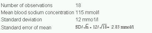
To find the 95% confidence interval above and below the mean we now have to find a multiple of the standard error. In large samples we have seen that the multiple is 1.96 (Chapter 4). For small samples we use the table of t given in Appendix Table B.pdf. As the sample becomes smaller t becomes larger for any particular level of probability. Conversely, as the sample becomes larger t becomes smaller and approaches the values given in table A, reaching them for infinitely large samples.
Since the size of the sample influences the value of t, the size of the sample is taken into account in relating the value of t to probabilities in the table. Some useful parts of the full t table appear in . The left hand column is headed d.f. for “degrees of freedom”. The use of these was noted in the calculation of the standard deviation (Chapter 2). In practice the degrees of freedom amount in these circumstances to one less than the number of observations in the sample. With these data we have 18 – 1 = 17 d.f. This is because only 17 observations plus the total number of observations are needed to specify the sample, the 18th being determined by subtraction.
To find the number by which we must multiply the standard error to give the 95% confidence interval we enter table B at 17 in the left hand column and read across to the column headed 0.05 to discover the number 2.110. The 95% confidence intervals of the mean are now set as follows:
Mean + 2.110 SE to Mean – 2.110 SE
which gives us:
115 – (2.110 x 283) to 115 + 2.110 x 2.83 or 109.03 to 120.97 mmol/l.
We may then say, with a 95% chance of being correct, that the range 109.03 to 120.97 mmol/l includes the population mean.
Likewise from Appendix Table B.pdf the 99% confidence interval of the mean is as follows:
Mean + 2.898 SE to Mean – 2.898 SE
which gives:
115 – (2.898 x 2.83) to 115 + (2.898 x 2.83) or 106.80 to 123.20 mmol/l.
Difference of sample mean from population mean (one sample t test)
Estimations of plasma calcium concentration in the 18 patients with Everley’s syndrome gave a mean of 3.2 mmol/l, with standard deviation 1.1. Previous experience from a number of investigations and published reports had shown that the mean was commonly close to 2.5 mmol/l in healthy people aged 20-44, the age range of the patients. Is the mean in these patients abnormally high?
We set the figures out as follows:
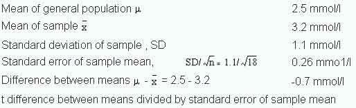
t difference between means divided by standard error of sample mean. Ignoring the sign of the t value, and entering table B at 17 degrees of freedom, we find that 2.69 comes between probability values of 0.02 and 0.01, in other words between 2% and 1% and so It is therefore unlikely that the sample with mean 3.2 came from the population with mean 2.5, and we may conclude that the sample mean is, at least statistically, unusually high. Whether it should be regarded clinically as abnormally high is something that needs to be considered separately by the physician in charge of that case.

Difference between means of two samples
Here we apply a modified procedure for finding the standard error of the difference between two means and testing the size of the difference by this standard error (see Chapter 5 for large samples). For large samples we used the standard deviation of each sample, computed separately, to calculate the standard error of the difference between the means. For small samples we calculate a combined standard deviation for the two samples.
The assumptions are:
- that the data are quantitative and plausibly Normal
- that the two samples come from distributions that may differ in their mean value, but not in the standard deviation
- that the observations are independent of each other.
- The third assumption is the most important. In general, repeated measurements on the same individual are not independent. If we had 20 leg ulcers on 15 patients, then we have only 15 independent observations.
The following example illustrates the procedure.
The addition of bran to the diet has been reported to benefit patients with diverticulosis. Several different bran preparations are available, and a clinician wants to test the efficacy of two of them on patients, since favourable claims have been made for each. Among the consequences of administering bran that requires testing is the transit time through the alimentary canal. Does it differ in the two groups of patients taking these two preparations?
The null hypothesis is that the two groups come from the same population. By random allocation the clinician selects two groups of patients aged 40-64 with diverticulosis of comparable severity. Sample 1 contains 15 patients who are given treatment A, and sample 2 contains 12 patients who are given treatment B. The transit times of food through the gut are measured by a standard technique with marked pellets and the results are recorded, in order of increasing time, in Table 7.1 .
Table 7.1
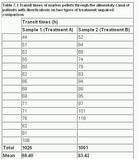
These data are shown in figure 7.1 . The assumption of approximate Normality and equality of variance are satisfied. The design suggests that the observations are indeed independent. Since it is possible for the difference in mean transit times for A-B to be positive or negative, we will employ a two sided test.
Figure 7.1
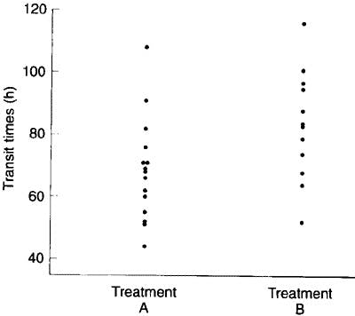
With treatment A the mean transit time was 68.40 h and with treatment B 83.42 h. What is the significance of the difference, 15.02h?
The procedure is as follows:
Obtain the standard deviation in sample 1: ![]()
Obtain the standard deviation in sample 2: ![]()
Multiply the square of the standard deviation of sample 1 by the degrees of freedom, which is the number of subjects minus one:
![]()
Repeat for sample 2
![]()
Add the two together and divide by the total degrees of freedom
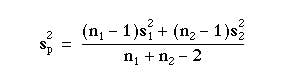
The standard error of the difference between the means is
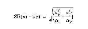
which can be written
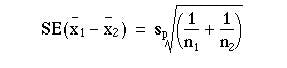
When the difference between the means is divided by this standard error the result is t. Thus, 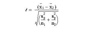
The table of the tdistribution Table B (appendix) which gives two sided P values is entered at degrees of freedom.
For the transit times of table 7.1,
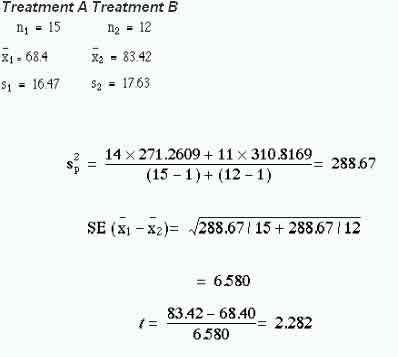 shows that at 25 degrees of freedom (that is (15 – 1) + (12 – 1)), t= 2.282 lies between 2.060 and 2.485. Consequently, this degree of probability is smaller than the conventional level of 5%. The null hypothesis that there is no difference between the means is therefore somewhat unlikely.
A 95% confidence interval is given by ![]() This becomes
This becomes
83.42 – 68.40 2.06 x 6.582
15.02 – 13.56 to 15.02 + 13.56 or 1.46 to 18.58 h.
Unequal standard deviations
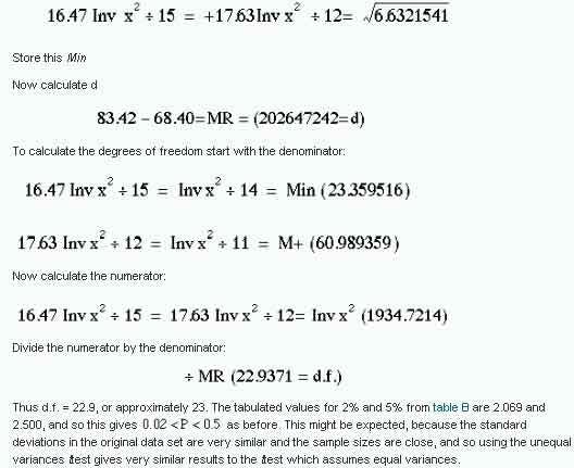
If the standard deviations in the two groups are markedly different, for example if the ratio of the larger to the smaller is greater than two, then one of the assumptions of the ttest (that the two samples come from populations with the same standard deviation) is unlikely to hold. An approximate test, due to Sattherwaite, and described by Armitage and Berry, (1)which allows for unequal standard deviations, is as follows.
Rather than use the pooled estimate of variance, compute
 This is analogous to calculating the standard error of the difference in two proportions under the alternative hypothesis as described in Chapter 6
We now compute  We then test this using a t statistic, in which the degrees of freedom are:
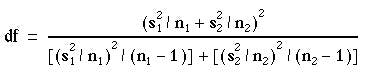
Although this may look very complicated, it can be evaluated very easily on a calculator without having to write down intermediate steps (see below). It can produce a degree of freedom which is not an integer, and so not available in the tables. In this case one should round to the nearest integer. Many statistical packages now carry out this test as the default, and to get the equal variances I statistic one has to specifically ask for it. The unequal variance t test tends to be less powerful than the usual t test if the variances are in fact the same, since it uses fewer assumptions. However, it should not be used indiscriminantly because, if the standard deviations are different, how can we interpret a nonsignificant difference in means, for example? Often a better strategy is to try a data transformation, such as taking logarithms as described in Chapter 2. Transformations that render distributions closer to Normality often also make the standard deviations similar. If a log transformation is successful use the usual t test on the logged data. Applying this method to the data of Table 7.1 , the calculator method (using a Casio fx-350) for calculating the standard error is:
Difference between means of paired samples (paired t test).
When the effects of two alternative treatments or experiments are compared, for example in cross over trials, randomised trials in which randomisation is between matched pairs, or matched case control studies (see Chapter 13 ), it is sometimes possible to make comparisons in pairs. Matching controls for the matched variables, so can lead to a more powerful study.
The test is derived from the single sample t test, using the following assumptions.
- The data are quantitative
- The distribution of the differences (not the original data), is plausibly Normal.
- The differences are independent of each other.
The first case to consider is when each member of the sample acts as his own control. Whether treatment A or treatment B is given first or second to each member of the sample should be determined by the use of the table of random numbers Table F (Appendix). In this way any effect of one treatment on the other, even indirectly through the patient’s attitude to treatment, for instance, can be minimised. Occasionally it is possible to give both treatments simultaneously, as in the treatment of a skin disease by applying a remedy to the skin on opposite sides of the body.
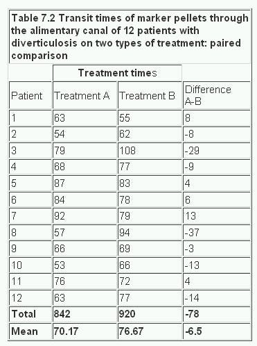
Let us use as an example the studies of bran in the treatment of diverticulosis discussed earlier. The clinician wonders whether transit time would be shorter if bran is given in the same dosage in three meals during the day (treatment A) or in one meal (treatment B). A random sample of patients with disease of comparable severity and aged 20-44 is chosen and the two treatments administered on two successive occasions, the order of the treatments also being determined from the table of random numbers. The alimentary transit times and the differences for each pair of treatments are set out in Table 7.2
Table 7.2
In calculating t on the paired observations we work with the difference, d, between the members of each pair. Our first task is to find the mean of the differences between the observations and then the standard error of the mean, proceeding as follows:
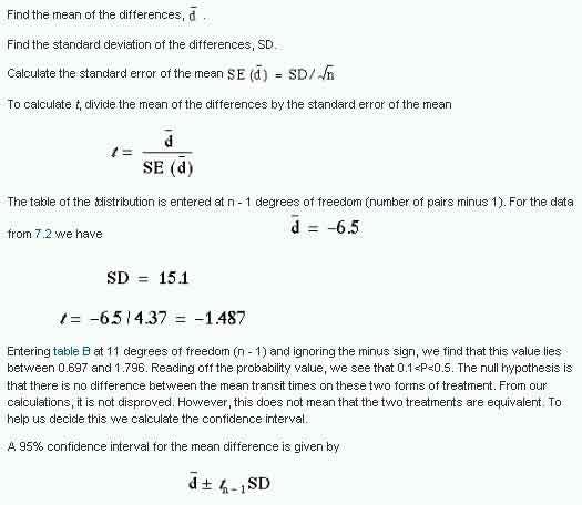
Entering Appendix Table B.pdf at 11 degrees of freedom (n – 1) and ignoring the minus sign, we find that this value lies between 0.697 and 1.796. Reading off the probability value, we see that 0.1
A 95% confidence interval for the mean difference is given by
![]()
In this case t 11 at P = 0.05 is 2.201 (table B) and so the 95% confidence interval is:
-6.5 – 2.201 x 4.37 to -6.5 + 2.201 x 4.37 h. or -16.1 to 3.1h.
This is quite wide, so we cannot really conclude that the two preparations are equivalent, and should look to a larger study.
The second case of a paired comparison to consider is when two samples are chosen and each member of sample 1 is paired with one member of sample 2, as in a matched case control study. As the aim is to test the difference, if any, between two types of treatment, the choice of members for each pair is designed to make them as alike as possible. The more alike they are, the more apparent will be any differences due to treatment, because they will not be confused with differences in the results caused by disparities between members of the pair. The likeness within the pairs applies to attributes relating to the study in question. For instance, in a test for a drug reducing blood pressure the colour of the patients’ eyes would probably be irrelevant, but their resting diastolic blood pressure could well provide a basis for selecting the pairs. Another (perhaps related) basis is the prognosis for the disease in patients: in general, patients with a similar prognosis are best paired. Whatever criteria are chosen, it is essential that the pairs are constructed before the treatment is given, for the pairing must be uninfluenced by knowledge of the effects of treatment.
Further methods
Suppose we had a clinical trial with more than two treatments. It is not valid to compare each treatment with each other treatment using t tests because the overall type I error rate will be bigger than the conventional level set for each individual test. A method of controlling for this to use a one way analysis of variance .(2)
Common questions
Should I test my data for Normality before using the t test?
It would seem logical that, because the t test assumes Normality, one should test for Normality first. The problem is that the test for Normality is dependent on the sample size. With a small sample a non-significant result does not mean that the data come from a Normal distribution. On the other hand, with a large sample, a significant result does not mean that we could not use the t test, because the t test is robust to moderate departures from Normality – that is, the P value obtained can be validly interpreted. There is something illogical about using one significance test conditional on the results of another significance test. In general it is a matter of knowing and looking at the data. One can “eyeball” the data and if the distributions are not extremely skewed, and particularly if (for the two sample t test) the numbers of observations are similar in the two groups, then the t test will be valid. The main problem is often that outliers will inflate the standard deviations and render the test less sensitive. Also, it is not generally appreciated that if the data originate from a randomised controlled trial, then the process of randomisation will ensure the validity of the I test, irrespective of the original distribution of the data.
Should I test for equality of the standard deviations before using the usual t test?
The same argument prevails here as for the previous question about Normality. The test for equality of variances is dependent on the sample size. A rule of thumb is that if the ratio of the larger to smaller standard deviation is greater than two, then the unequal variance test should be used. With a computer one can easily do both the equal and unequal variance t test and see if the answers differ.
Why should I use a paired test if my data are paired? What happens if I don’t?
Pairing provides information about an experiment, and the more information that can be provided in the analysis the more sensitive the test. One of the major sources of variability is between subjects variability. By repeating measures within subjects, each subject acts as its own control, and the between subjects variability is removed. In general this means that if there is a true difference between the pairs the paired test is more likely to pick it up: it is more powerful. When the pairs are generated by matching the matching criteria may not be important. In this case, the paired and unpaired tests should give similar results.
References
- Armitage P, Berry G. Statistical Methods in Medical Research. 3rd ed. Oxford: Blackwell Scientific Publications, 1994:112-13.
- Armitage P, Berry G. Statistical Methods in Medical Research. 3rd ed. Oxford: Blackwell Scientific Publications, 1994:207-14.
Exercises
7.1 In 22 patients with an unusual liver disease the plasma alkaline phosphatase was found by a certain laboratory to have a mean value of 39 King-Armstrong units, standard deviation 3.4 units. What is the 95% confidence interval within which the mean of the population of such cases whose specimens come to the same laboratory may be expected to lie?
7.2 In the 18 patients with Everley’s syndrome the mean level of plasma phosphate was 1.7 mmol/l, standard deviation 0.8. If the mean level in the general population is taken as 1.2 mmol/l, what is the significance of the difference between that mean and the mean of these 18 patients?
7.3 In two wards for elderly women in a geriatric hospital the following levels of haemoglobin were found:
Ward A: 12.2, 11.1, 14.0, 11.3, 10.8, 12.5, 12.2, 11.9, 13.6, 12.7, 13.4, 13.7 g/dl;
Ward B: 11.9, 10.7, 12.3, 13.9, 11.1, 11.2, 13.3, 11.4, 12.0, 11.1 g/dl.
What is the difference between the mean levels in the two wards, and what is its significance? What is the 95% confidence interval for the difference in treatments?
7.4 A new treatment for varicose ulcer is compared with a standard treatment on ten matched pairs of patients, where treatment between pairs is decided using random numbers. The outcome is the number of days from start of treatment to healing of ulcer. One doctor is responsible for treatment and a second doctor assesses healing without knowing which treatment each patient had. The following treatment times were recorded.
Standard treatment: 35, 104, 27, 53, 72, 64, 97, 121, 86, 41 days;
New treatment: 27, 52, 46, 33, 37, 82, 51, 92, 68, 62 days.
What are the mean difference in the healing time, the value of t, the number of degrees of freedom, and the probability? What is the 95% confidence interval for the difference?
When do we use one-sample t-test?
The one-sample t-test is a very simple statistical test. It is used when we have a sample of numeric variable, and we want to compare its population mean to a particular value. The one-sample t-test evaluates whether the population mean is likely to be different from this value. The expected value could be any value we are interested in. Here are a couple of specific examples:
-
We have developed a theoretical model of foraging behaviour that predicts an animal should leave a food patch after 10 minutes. If we have data on the actual time spent by 25 animals observed foraging in the patch, we could test whether the mean foraging time is ‘significantly different’ from the prediction using a one-sample t-test.
-
We are monitoring sea pollution and have collected a series of water samples from a beach. We wish to test whether the mean density of faecal coliforms—bacteria indicative of sewage discharge—can be regarded as greater than the legislated limit. A one-sample t-test will test whether the mean value for the beach as a whole exceeds this limit.
Let’s see if we can get sense of how these tests would work.
How does the one-sample t-test work?
Imagine we have taken a sample of some variable and we want to evaluate whether its mean is different from some number (the ‘expected value’).
Here’s an example of what these data might look like if we had used a sample size of 50:
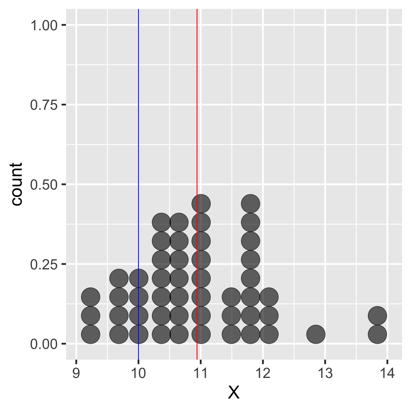
Figure 12.1: Example of data used in a one-sample t-test
We’re calling the variable ‘X’ in this example. It needs a label and ‘X’ is as good as any other. The red line shows the sample mean. This is a bit less than 11. The blue line shows the expected value. This is 10, so this example could correspond to the foraging study mentioned above.
The observed sample mean is about one unit larger than the expected value. The question is, how do we decide whether the population mean is really different from the expected value? Perhaps the difference between the observed and expected value is due to sampling variation. Here’s how a frequentist tackles this kind of question:
-
Set up an appropriate null hypothesis, i.e. an hypothesis of ‘no effect’ or ‘no difference.’ The null hypothesis in this type of question is that the population mean is equal to the expected value.
-
Work out what the sampling distribution of a sample mean looks like under the null hypothesis. This is the null distribution. Because we’re now using a parametric approach, we will assume this has a particular form.
-
Finally, we use the null distribution to assess how likely the observed result is under the null hypothesis. This is the p-value calculation that we use to summarise our test.
This chain of reasoning is no different from that developed in the bootstrapping example from earlier. We’re just going to make an extra assumption this time to allow us to use a one-sample t-test. This extra assumption is that the variable (‘X’) is normally distributed in the population. When we make this normality assumption the whole process of carrying out the statistical test is actually very simple because the null distribution will have a known mathematical form—it ends up being a t-distribution.
We can use this knowledge to construct the test of statistical significance. Instead of using the whole sample, as we did with the bootstrap, now we only need three simple pieces of information to construct the test: the sample size, the sample variance, and the sample mean. The one-sample t-test is then carried out as follows:
Step 1. Calculate the sample mean. This happens to be our ‘best guess’ of the unknown population mean. However, its role in the one-sample t-test is to allow us to construct a test statistic in the next step.
Step 2. Estimate the standard error of the sample mean. This gives us an idea of how much sampling variation we expect to observe. The standard error doesn’t depend on the true value of the mean, so the standard error of the sample mean is also the standard error of any mean under any particular null hypothesis.
This second step boils down to applying a simple formula involving the sample size and the standard deviation of the sample:
[text{Standard Error of the Mean} = sqrt{frac{s^2}{n}}]
…where (s^2) is the square of the standard deviation (the sample variance) and (n) is for the sample size. This is the formula introduced in the parametric statistics chapter. The standard error of the mean gets smaller as the sample sizes grows or the sample variance shrinks.
Step 3. Calculate a ‘test statistic’ from the sample mean and standard error. We calculate this by dividing the sample mean (step 1) by its estimated standard error (step 2):
[text{t} = frac{text{Sample Mean}}{text{Standard Error of the Mean}}]
If our normality assumption is reasonable this test-statistic follows a t-distribution. This is guaranteed by the normality assumption. So this particular test statistic is also a t-statistic. That’s why we label it t. This knowledge leads to the final step…
Step 4. Compare the t-statistic to the theoretical predictions of the t-distribution to assess the statistical significance of the difference between observed and expected value. We calculate the probability that we would have observed a difference with a magnitude as large as, or larger than, the observed difference, if the null hypothesis were true. That’s the p-value for the test.
We could step through the actual calculations involved in these steps in detail, using R to help us, but there’s no need to do this. We can let R handle everything for us. But first, we should review the assumptions of the one-sample t-test.
Assumptions of the one-sample t-test
There are a number of assumptions that need to be met in order for a one-sample t-test to be valid. Some of these are more important than others. We’ll start with the most important and work down the list in reverse order of importance:
- Independence. In rough terms, independence means each observation in the sample does not ‘depend on’ the others. We’ll discuss this more carefully when we consider the principles of experimental design. The key thing to know now is why this assumption matters: if the data are not independent the p-values generated by the one-sample t-test will be unreliable.
(In fact, the p-values will be too small when the non-independence assumption is broken. That means we risk the false conclusion that a difference is statistically significant, when in reality, it is not)
-
Measurement scale. The variable being analysed should be measured on an interval or ratio scale, i.e. it should be a numeric variable of some kind. It doesn’t make much sense to apply a one-sample t-test to a variable that isn’t measured on one of these scales.
-
Normality. The one-sample t-test will only produce completely reliable p-values when the variable is normally distributed in the population. However, this assumption is less important than many people think. The t-test is robust to mild departures from normality when the sample size is small, and when the sample size is large the normality assumption hardly matters at all.
We don’t have the time to explain why the normality assumption is not too important for large samples, but we can at least state the reason: it is a consequence of that central limit theorem we mentioned in the last chapter.
Evaluating the assumptions
The first two assumptions—independence and measurement scale—are really aspects of experimental design. We can only evaluate these by thinking carefully about how the data were gathered and what was measured. It’s too late to do anything about these after we have collected our data.
What about that 3rd assumption—normality? One way to evaluate this is by visualising the sample distribution. For small samples, if the sample distribution looks approximately normal then it’s probably fine to use the t-test. For large samples, we don’t even need to worry about a moderate departures from normality3.
Carrying out a one-sample t-test in R
You should work through the example in this section if you have time. Carry on developing the script you began in the last chapter, or if you prefer, set up a script. Everything below assumes you have read the data in MORPH_DATA.CSV into an R data frame called morph_data.
We’ll use the plant morph example again to learn how to carry out a one-sample t-test in R. Remember, the data were ‘collected’ to 1) compare the frequency of purple morphs to a prediction and 2) compare the mean dry weight of purple and green morphs. Neither of these questions can be tackled with a one-sample t-test.
Instead, let’s pretend that we unearthed a report from 30 years ago that found the mean size of purple morphs to be 710 grams. We want to evaluate whether the mean size of purple plants in the contemporary population is different from this expectation, because we think they may have adapted to local conditions.
We only need the purple morph data for this example so we should first filter the data to get hold of only the purple plants:
# get just the purple morphs
purple_morphs <- filter(morph_data, Colour == "Purple")
The purple_morphs data set has two columns: Weight contains the dry weight biomass of purple plants and Colour indicates which sample (plant morph) an observation belongs to. We don’t need the Colour column any more because we’ve just removed all the green plants but there’s no harm in leaving it in.
Visualising the data and checking the assumptions
We start by calculating a few summary statistics and visualising the sample distribution of purple morph dry weights. That’s right… always check the data before carrying out any kind of statistical analysis! We already looked over these data in the Statistical comparisons chapter. We’ll proceed as though this is the first time we’ve seen them though to demonstrate the complete work flow.
Here is the dplyr code to produce the descriptive statistics:
purple_morphs %>%
  summarise(mean = mean(Weight),
            sd = sd(Weight),
            samp_size = n())
## # A tibble: 1 x 3
## mean sd samp_size
## <dbl> <dbl> <int>
## 1 767. 156. 77We have 77 purple plants in the sample. Not bad but we should keep an eye on the normality assumption. Let’s check this by making a histogram with the sample of purple plant dry weights:
ggplot(purple_morphs, aes(x = Weight)) +
  geom_histogram(binwidth = 50)
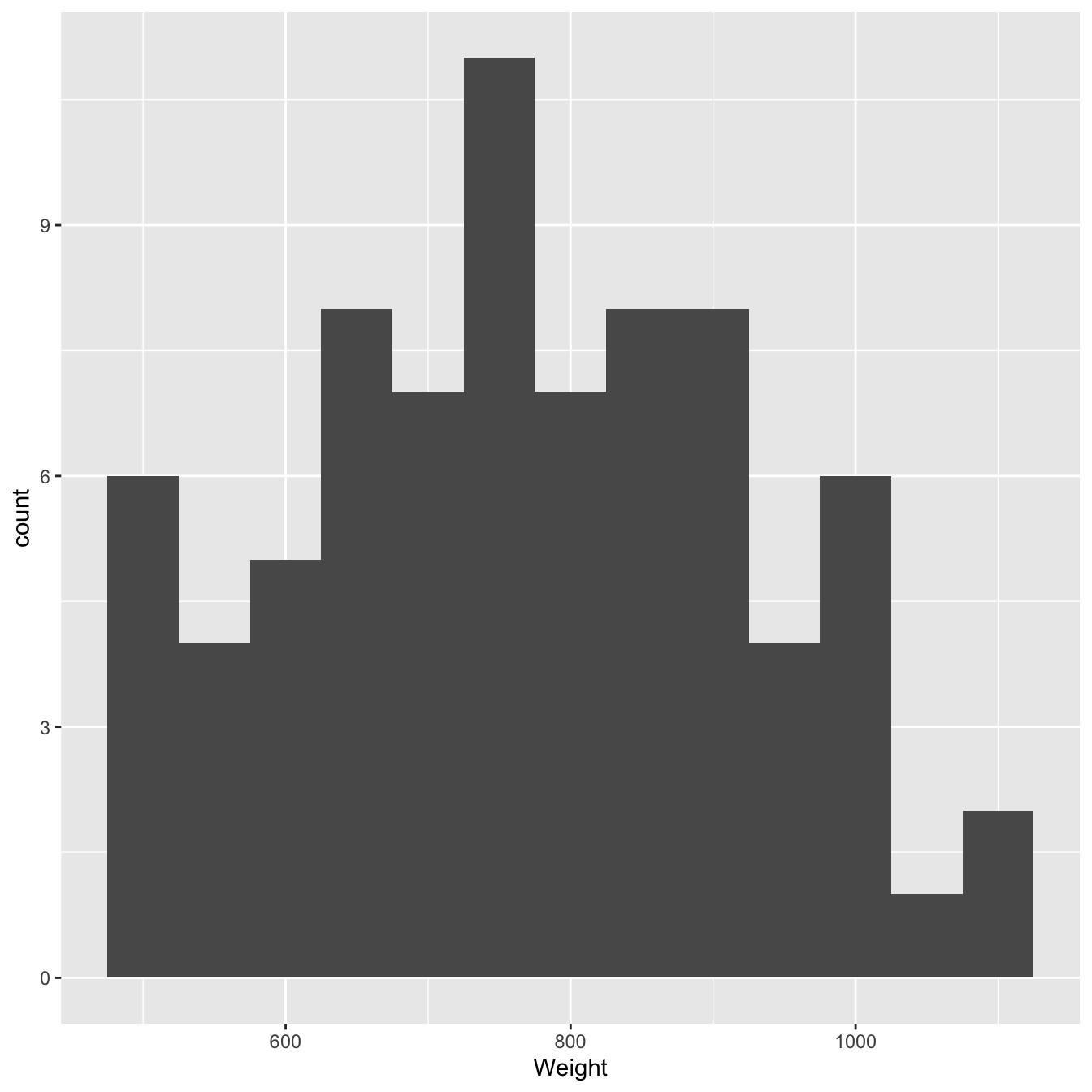
Figure 12.2: Size distributions of purple morph dry weight sample
These is nothing too ‘non-normal’ about this sample distribution—it’s roughly bell-shaped—so it seems reasonable to assume it came from normally distributed population.
Carrying out the test
It’s easy to carry out a one-sample t-test in R. The function we use is called t.test (no surprises there). Remember, Weight contains the dry weight biomass of purple plants. Here’s the R code to carry out a one-sample t-test:
t.test(purple_morphs$Weight, mu = 710)We have suppressed the output because we want to initially focus on how to use the t.test function. We have to assign two arguments to control what the function does:
-
The first argument (
purple_morphs$Weight) is simply a numeric vector containing the sample values. Sadly we can’t givet.testa data frame when doing a one-sample test. Instead, we have to pull out the column we’re interested in using the$operator. -
The second argument (called
mu) sets the expected value we want to compare the sample mean to. Somu = 710tells the function to compare the sample mean to a value of 710. This can be any value we like and the correct value depends on the question we’re asking.
That’s it for setting up the test. Here is the R code for the test again, this time with the output included:
t.test(purple_morphs$Weight, mu = 710)##
## One Sample t-test
##
## data: purple_morphs$Weight
## t = 3.1811, df = 76, p-value = 0.002125
## alternative hypothesis: true mean is not equal to 710
## 95 percent confidence interval:
## 731.1490 801.9787
## sample estimates:
## mean of x
## 766.5638The first line tells us what kind of t-test we used. This says: One Sample t-test. OK, now we know that we used the one-sample t-test (there are other kinds). The next line reminds us about the data. This says: data: purple_morphs$Weight, which is R-speak for ’we compared the mean of the Weight variable to an expected value. Which value? This is given later.
The third line of text is the most important. This says: t = 3.1811, df = 76, p-value = 0.002125. The first part of this, t = 3.1811, is the test statistic, i.e. the value of the t-statistic. The second part, df = 76, summarise the ‘degrees of freedom.’ This is required to work out the p-value. It also tells us something about how much ‘power’ our statistical test has (see the box below). The third part, p-value = 0.002125, is the all-important p-value.
That p-value indicates that there is a statistically significant difference between the mean dry weight biomass and the expected value of 710 g (p is less than 0.05). Because the p-value is less than 0.01 but greater than 0.001, we report this as ‘p < 0.01.’ Read through the Presenting p-values section again if this logic is confusing.
The fourth line of text (alternative hypothesis: true mean is not equal to 710) tells us what the alternative to the null hypothesis is (H1). More importantly, this serves to remind us which expected value was used to formulate the null hypothesis (mean = 710).
The next two lines show us the ‘95% confidence interval’ for the difference between the means. We don’t really need this information now, but we can think of this interval as a rough summary of the likely values of the ‘true’ mean4.
The last few lines summarise the sample mean. This might be useful if we had not already calculated.
A bit more about degrees of freedom
Degrees of freedom (abbreviated d.f. or df) are closely related to the idea of sample size. The greater the degrees of freedom associated with a test, the more likely it is to detect an effect if it’s present. To calculate the degrees of freedom, we start with the sample size and then we reduce this number by one for every quantity (e.g. a mean) we had to calculate to construct the test.
Calculating degrees of freedom for a one-sample t-test is easy. The degrees of freedom are just n-1, where n is the number of observations in the sample. We lose one degree of freedom because we have to calculate one sample mean to construct the test.
Summarising the result
Having obtained the result we now need to write our conclusion. We are testing a scientific hypothesis, so we must always return to the original question to write the conclusion. In this case the appropriate conclusion is:
The mean dry weight biomass of purple plants is significantly different from the expectation of 710 grams (t = 3.18, d.f. = 76, p < 0.01).
This is a concise and unambiguous statement in response to our initial question. The statement indicates not just the result of the statistical test, but also which value was used in the comparison. It is sometimes appropriate to give the values of the sample mean in the conclusion:
The mean dry weight biomass of purple plants (767 grams) is significantly different from the expectation of 710 grams (t = 3.18, d.f. = 76, p < 0.01).
Notice that we include details of the test in the conclusion. However, keep in mind that when writing scientific reports, the end result of any statistical test should be a conclusion like the one above. Simply writing t = 3.18 or p < 0.01 is not an adequate conclusion.
There are a number of common questions that arise when presenting t-test results:
-
What do I do if t is negative? Don’t worry. A t-statistic can come out negative or positive, it simply depends on which order the two samples are entered into the analysis. Since it is just the absolute value of t that determines the p-value, when presenting the results, just ignore the minus sign and always give t as a positive number.
-
How many significant figures for t? The t-statistic is conventionally given to 3 significant figures. This is because, in terms of the p-value generated, there is almost no difference between, say, t = 3.1811 and t = 3.18.
-
Upper or lower case The t statistic should always be written as lower case when writing it in a report (as in the conclusions above). Similarly, d.f. and p are always best as lower case. Some statistics we encounter later are written in upper case but, even with these, d.f. and p should be lower case.
-
How should I present p? There are various conventions in use for presenting p-values. We discussed these in the Hypotheses and p-values chapter. Learn them! It’s not possible to understand scientific papers or prepare reports properly without knowing these conventions.
p = 0.00? It’s impossible! p = 1e-16? What’s that?
Some statistics packages will sometimes give a probability of p = 0.00. This does not mean the probability was actually zero. A probability of zero would mean an outcome was impossible, even though it happened! When a computer package reports p = 0.00 it just means that the probability was ‘very small’ and ended up being rounded down to 0.
R typically uses a slightly different convention for presenting small probabilities. A very small probability is given as p-value < 2.2e-16. What does 2.2e-16 mean? This is R-speak for scientific notation, i.e. (2.2e^{-16}) is equivalent to (2.2 times 10^{-16}).
Keep in mind that we should report a result like this as p < 0.001; do not write something like p = 2.2e-16.
The t-test procedure performs t-tests for one sample, two samples and
paired observations. The single-sample t-test compares the mean of the sample
to a given number (which you supply). The independent samples t-test compares
the difference in the means from the two groups to a given value (usually 0).
In other words, it tests whether the difference in the means is 0. The
dependent-sample or paired t-test compares the difference in the means from the
two variables measured on the same set of subjects to a given number (usually
0), while taking into account the fact that the scores are not independent. In
our examples, we will use the hsb2
data set.
Single sample t-test
The single sample t-test tests the null hypothesis that the population mean
is equal to the number specified by the user. SPSS calculates the t-statistic
and its p-value under the assumption that the sample comes from an approximately
normal distribution. If the p-value associated with the t-test is small (0.05 is
often used as the threshold), there is evidence that the mean is different from
the hypothesized value. If the p-value associated with the t-test is not small
(p > 0.05), then the null hypothesis is not rejected and you can conclude that
the mean is not different from the hypothesized value.
In this example, the t-statistic is 4.140 with 199 degrees of freedom. The
corresponding two-tailed p-value is .000, which is less than 0.05. We conclude
that the mean of variable write is different from 50.
get file "C:datahsb2.sav".
t-test
/testval=50
variables=write.
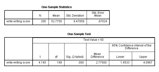
One-Sample Statistics
a. – This is the list of variables. Each variable
that was listed on the variables= statement in the above code will have its own line in this part
of the output.
b. N – This is the number of valid (i.e., non-missing)
observations used in calculating the t-test.
c. Mean – This is the mean of the variable.
d. Std. Deviation – This is the standard deviation of the variable.
e. Std. Error Mean – This is the estimated standard deviation of
the sample mean. If we drew repeated samples of size 200, we would expect the
standard deviation of the sample means to be close to the standard error. The
standard deviation of the distribution of sample mean is estimated as the
standard deviation of the sample divided by the square root of sample size:
9.47859/(sqrt(200)) = .67024.
Test statistics
f. – This identifies the variables. Each variable
that was listed on the variables= statement will have its own line in this part
of the output. If a variables= statement is not specified, t-test will
conduct a t-test on all numerical variables in the dataset.
g. t – This is the Student t-statistic. It is the ratio of the
difference between the sample mean and the given number to the standard error of
the mean: (52.775 – 50) / .6702372 = 4.1403. Since the standard error of the
mean measures the variability of the sample mean, the smaller the standard error
of the mean, the more likely that our sample mean is close to the true
population mean. This is illustrated by the following three figures.
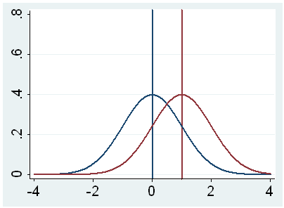
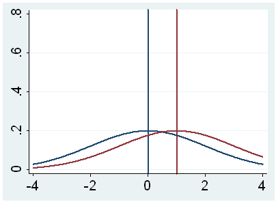
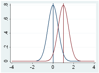
In all three cases, the difference between the population means is the same.
But with large variability of sample means, second graph, two populations
overlap a great deal. Therefore, the difference may well come by chance. On
the other hand, with small variability, the difference is more clear as in the
third graph. The smaller the standard error of the mean, the larger the
magnitude of the t-value and therefore, the smaller the p-value.
h. df – The degrees of freedom for the single sample t-test is simply
the number of valid observations minus 1. We loose one degree of freedom
because we have estimated the mean from the sample. We have used some of the
information from the data to estimate the mean, therefore it is not available to
use for the test and the degrees of freedom accounts for this.
i. Sig (2-tailed)– This is the two-tailed p-value
evaluating the null against an alternative that the mean is not equal to 50.
It is equal to the probability of observing a greater absolute value of t under
the null hypothesis. If the p-value is less than the pre-specified alpha
level (usually .05 or .01) we will conclude that mean is statistically
significantly different from zero. For example, the p-value is smaller than 0.05.
So we conclude that the mean for write is different from 50.
j. Mean Difference – This is the difference between the sample
mean and the test value.
k. 95% Confidence Interval of the Difference – These are the
lower and upper bound of the confidence interval for the mean. A confidence
interval for the mean specifies a range of values within which the unknown
population parameter, in this case the mean, may lie. It is given by
![]()
where s is the sample deviation of the observations and N is the number of valid
observations. The t-value in the formula can be computed or found in any
statistics book with the degrees of freedom being N-1 and the p-value being 1-alpha/2,
where alpha is the confidence level and by default is .95.
Paired t-test
A paired (or “dependent”) t-test is used when the observations are not
independent of one another. In the example below, the same students took both
the writing and the reading test. Hence, you would expect there to be a
relationship between the scores provided by each student. The paired t-test
accounts for this. For each student, we are essentially looking at the
differences in the values of the two variables and testing if the mean of these
differences is equal to zero.
In this example, the t-statistic is 0.8673 with 199 degrees of freedom. The
corresponding two-tailed p-value is 0.3868, which is greater than 0.05. We
conclude that the mean difference of write and read is not
different from 0.
t-test
pairs=write with read (paired).
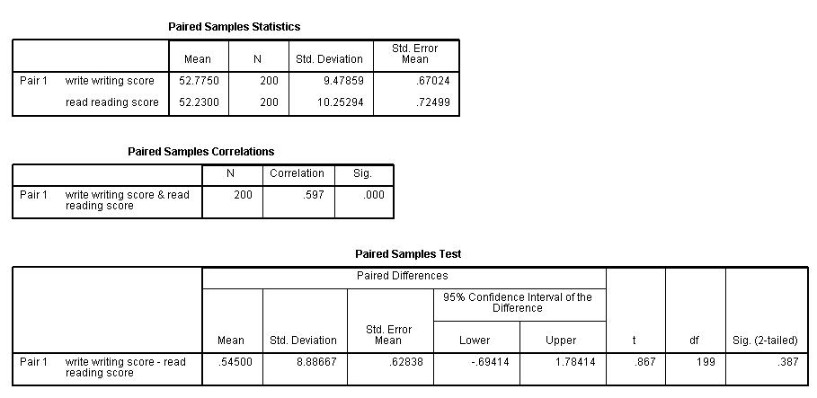
Summary statistics
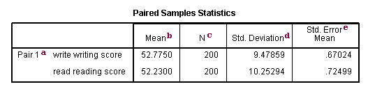
a. – This is the list of variables.
b. Mean – These are the
respective means of the variables.
c. N – This is the number of valid (i.e., non-missing)
observations used in calculating the t-test.
d. Std. Deviation – This is the standard deviations of the variables.
e. Std Error Mean – Standard Error Mean is the estimated standard deviation of the
sample mean. This value is estimated as the standard deviation of one sample divided by
the square root of sample size: 9.47859/sqrt(200) = .67024, 10.25294/sqrt(200) = .72499.
This provides a measure of the variability of the sample mean.
f. Correlation – This is the correlation coefficient of the pair of
variables indicated. This is a measure of the strength and direction
of the linear relationship between the two variables. The correlation
coefficient can range from -1 to +1, with -1 indicating a perfect negative
correlation, +1 indicating a perfect positive correlation, and 0 indicating no
correlation at all. (A variable correlated with itself will always have a
correlation coefficient of 1.) You can think of the correlation
coefficient as telling you the extent to which you can guess the value of one
variable given a value of the other variable. The .597 is the numerical description of how
tightly around the imaginary line the points lie. If the correlation was higher, the points would
tend to be closer to the line; if it was smaller, they would tend to be further
away from the line.
g. Sig – This is the p-value associated with the correlation.
Here, correlation is significant at the .05 level.
Test statistics
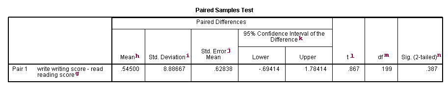
g. writing score-reading score – This is the value measured
within each subject: the difference between the writing and reading scores. The
paired t-test forms a single random sample of the paired difference. The mean of
these values among all subjects is compared to 0 in a paired t-test.
h. Mean – This is the mean within-subject difference between the two variables.
i. Std. Deviation – This is the standard deviation of the
mean paired difference.
j. Std Error Mean – This is the estimated standard deviation of the
sample mean. This value is estimated as the standard deviation of one sample divided
by the square root of sample size: 8.88667/sqrt(200) = .62838. This provides a measure
of the variability of the sample mean.
k. 95% Confidence Interval of the Difference – These are the
lower and upper bound of the confidence interval for the mean difference. A
confidence interval for the mean specifies a range of values within which the
unknown population parameter, in this case the mean, may lie. It is given
by
![]()
where s is the sample deviation of the observations and N is the number of valid
observations. The t-value in the formula can be computed or found in any
statistics book with the degrees of freedom being N-1 and the p-value being 1-alpha/2,
where alpha is the confidence level and by default is .95.
l. t – This is the t-statistic. It is the ratio of
the mean of the difference to the standard error of the difference: (.545/.62838).
m. degrees of freedom – The degrees of freedom for the paired observations is
simply the number of observations minus 1. This is because the test is conducted
on the one sample of the paired differences.
n. Sig. (2-tailed) –
This is the two-tailed p-value computed using the t distribution. It is
the probability of observing a greater absolute value of t under the null
hypothesis. If the p-value is less than the pre-specified alpha level
(usually .05 or .01, here the former) we will conclude that mean difference
between writing score and reading score is statistically significantly different from
zero. For example, the p-value for the difference between the two
variables
is greater than 0.05 so we conclude that the mean difference is not
statistically significantly different from 0.
Independent group t-test
This t-test is designed to compare means of same variable between two groups.
In our example, we compare the mean writing score between the group of
female students and the group of male students. Ideally, these subjects are
randomly selected from a larger population of subjects. The test assumes that
variances for the two populations are the same. The interpretation for p-value is the same as
in other type of t-tests.
In this example, the t-statistic is -3.7341 with 198 degrees of freedom. The corresponding
two-tailed p-value is 0.0002, which is less than 0.05. We conclude that
the difference of means in write between males and females is different
from 0.
t-test groups=female(0 1)
/variables=write.
Summary statistics
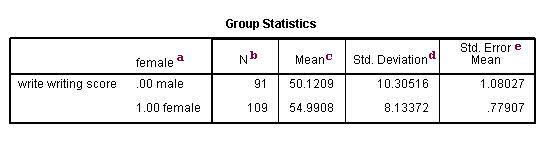
a. female – This column gives categories of
the independent variable female. This variable is necessary for
doing the independent group t-test and is specified by the t-test groups= statement.
b. N – This is the number of valid (i.e., non-missing) observations in each group.
c. Mean – This is the mean of the dependent variable for each
level of the independent variable.
d. Std. Deviation – This is the standard deviation of the
dependent variable for each of the levels of the independent variable.
e. Std. Error Mean – This is the standard error of the mean, the
ratio of the standard deviation to the square root of the respective number of
observations.
Test statistics
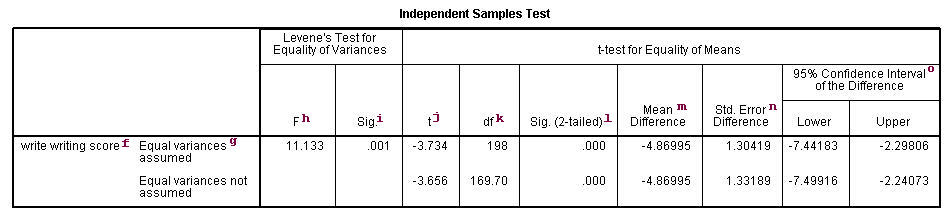
f. – This column lists the dependent variable(s). In
our example, the dependent variable is write (labeled “writing score”).
g. – This column specifies the method for computing the
standard error of the difference of the means. The method of computing
this value is based on the assumption regarding the
variances of the two groups. If we assume that the two populations have the same variance,
then the first method, called pooled variance estimator, is used. Otherwise, when
the variances are not assumed to be equal, the Satterthwaite’s method is used.
h. F– This column lists Levene’s test statistic. Assume (k) is the number of groups, (N) is the total number of observations, and (N_i) is the number of observations in each (i)-th group for dependent variable (Y_{ij}). Then Levene’s test statistic is defined as
begin{equation}
W = frac{(N-k)}{(k-1)} frac{sum_{i=1}^{k} N_i (bar{Z}_{i.}-bar{Z}_{..})^2}{sum_{i=1}^{k}sum_{j=1}^{N_i}(Z_{ij}-bar{Z}_{i.})^2}
end{equation}
begin{equation}
Z_{ij} = |Y_{ij}-bar{Y}_{i.}|
end{equation}
where (bar{Y}_{i.}) is the mean of the dependent variable and (bar{Z}_{i.}) is the mean of (Z_{ij}) for each (i)-th group respectively, and (bar{Z}_{..}) is the grand mean of (Z_{ij}).
i. Sig. – This is the two-tailed p-value associated with the null
that the two groups have the same variance. In our example, the probability is less
than 0.05. So there is evidence that the variances for the two groups, female
students and male students, are different. Therefore, we may want to use the
second method (Satterthwaite variance estimator) for our t-test.
j. t – These are the t-statistics under the two different
assumptions: equal variances and unequal variances. These are the ratios
of the mean of the differences to the standard errors of the difference under
the two different assumptions:
(-4.86995 / 1.30419) = -3.734, (-4.86995/1.33189) = -3.656.
k. df – The degrees of freedom when we assume equal variances is
simply the sum of the two sample sized (109 and 91) minus 2. The degrees of
freedom when we assume unequal variances is calculated using the Satterthwaite
formula.
l. Sig. (2-tailed) – The p-value is the two-tailed probability
computed using the t distribution. It is the probability of observing a t-value of
equal or greater absolute value under the null hypothesis. For a
one-tailed test, halve this probability. If the p-value is less than our
pre-specified alpha level, usually 0.05, we will conclude that the difference is significantly
different from zero. For example, the p-value for the difference between females and
males is less than 0.05 in both cases, so we conclude that the difference in means is statistically
significantly different from 0.
m. Mean Difference – This is the difference between the means.
n. Std Error Difference – Standard Error difference is the estimated standard deviation of the
difference between the sample means. If we drew repeated samples of size 200, we would expect the
standard deviation of the sample means to be close to the standard error.
This provides a measure of the variability of the sample mean. The Central
Limit Theorem tells us that the sample means are approximately normally
distributed when the sample size is 30 or greater. Note that the standard
error difference is calculated differently under the two different assumptions.
o. 95% Confidence Interval of the Difference – These are the
lower and upper bound of the confidence interval for the mean difference. A
confidence interval for the mean specifies a range of values within which the
unknown population parameter, in this case the mean, may lie. It is given
by
![]()
where s is the sample deviation of the observations and N is the number of valid
observations. The t-value in the formula can be computed or found in any
statistics book with the degrees of freedom being N-1 and the p-value being 1-width/2,
where width is the confidence level and by default is .95.
The ultimate guide to t tests
The t test is one of the simplest statistical techniques that is used to evaluate whether there is a statistical difference between the means from up to two different samples. The t test is especially useful when you have a small number of sample observations (under 30 or so), and you want to make conclusions about the larger population.
The characteristics of the data dictate the appropriate type of t test to run. All t tests are used as standalone analyses for very simple experiments and research questions as well as to perform individual tests within more complicated statistical models such as linear regression.
In this guide, we’ll lay out everything you need to know about t tests, including providing a simple workflow to determine what t test is appropriate for your particular data or if you’d be better suited using a different model.
What is a t test?
A t test is a statistical technique used to quantify the difference between the mean (average value) of a variable from up to two samples (datasets). The variable must be numeric. Some examples are height, gross income, and amount of weight lost on a particular diet.
A t test tells you if the difference you observe is “surprising” based on the expected difference. They use t-distributions to evaluate the expected variability. When you have a reasonable-sized sample (over 30 or so observations), the t test can still be used, but other tests that use the normal distribution (the z test) can be used in its place.
Sometimes t tests are called “Student’s” t tests, which is simply a reference to their unusual history.

It got its name because a brewer from the Guinness Brewery, William Gosset, published about the method under the pseudonym «Student». He wanted to get information out of very small sample sizes (often 3-5) because it took so much effort to brew each keg for his samples.
When should I use a t test?
A t test is appropriate to use when you’ve collected a small, random sample from some statistical “population” and want to compare the mean from your sample to another value. The value for comparison could be a fixed value (e.g., 10) or the mean of a second sample.
For example, if your variable of interest is the average height of sixth graders in your region, then you might measure the height of 25 or 30 randomly-selected sixth graders. A t test could be used to answer questions such as, “Is the average height greater than four feet?”
How does a t test work?
Based on your experiment, t tests make enough assumptions about your experiment to calculate an expected variability, and then they use that to determine if the observed data is statistically significant. To do this, t tests rely on an assumed “null hypothesis.” With the above example, the null hypothesis is that the average height is less than or equal to four feet.
Say that we measure the height of 5 randomly selected sixth graders and the average height is five feet. Does that mean that the “true” average height of all sixth graders is greater than four feet or did we randomly happen to measure taller than average students?
To evaluate this, we need a distribution that shows every possible average value resulting from a sample of five individuals in a population where the true mean is four. That may seem impossible to do, which is why there are particular assumptions that need to be made to perform a t test.
With those assumptions, then all that’s needed to determine the “sampling distribution of the mean” is the sample size (5 students in this case) and standard deviation of the data (let’s say it’s 1 foot).
That’s enough to create a graphic of the distribution of the mean, which is:
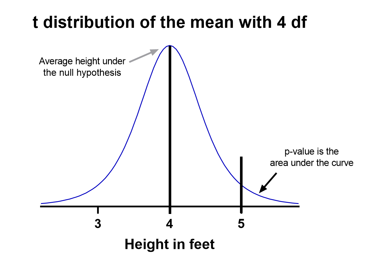
Notice the vertical line at x = 5, which was our sample mean. We (use software to) calculate the area to the right of the vertical line, which gives us the P value (0.09 in this case). Note that because our research question was asking if the average student is greater than four feet, the distribution is centered at four. Since we’re only interested in knowing if the average is greater than four feet, we use a one-tailed test in this case.
Using the standard confidence level of 0.05 with this example, we don’t have evidence that the true average height of sixth graders is taller than 4 feet.
What are the assumptions for t tests?
- One variable of interest: This is not correlation or regression, where you are interested in the relationship between multiple variables. With a t test, you can have different samples, but they are all measuring the same variable (e.g., height).
- Numeric data: You are dealing with a list of measurements that can be averaged. This means you aren’t just counting occurrences in various categories (e.g., eye color or political affiliation).
- Two groups or less: If you have more than two samples of data, a t test is the wrong technique. You most likely need to try ANOVA.
- Random sample: You need a random sample from your statistical “population of interest” in order to draw valid conclusions about the larger population. If your population is so small that you can measure everything, then you have a “census” and don’t need statistics. This is because you don’t need to estimate the truth, since you have measured the truth without variability.
- Normally Distributed: The smaller your sample size, the more important it is that your data come from a normal, Gaussian distribution bell curve. If you have reason to believe that your data are not normally distributed, consider nonparametric t test alternatives. This isn’t necessary for larger samples (usually 25 or 30 unless the data is heavily skewed). The reason is that the Central Limit Theorem applies in this case, which says that even if the distribution of your data is not normal, the distribution of the mean of your data is, so you can use a z-test rather than a t test.
How do I know which t test to use?
There are many types of t tests to choose from, but you don’t necessarily have to understand every detail behind each option.
You just need to be able to answer a few questions, which will lead you to pick the right t test. To that end, we put together this workflow for you to figure out which test is appropriate for your data.
Do you have one or two samples?
Are you comparing the means of two different samples, or comparing the mean from one sample to a fixed value? An example research question is, “Is the average height of my sample of sixth grade students greater than four feet?”
If you only have one sample of data, you can click here to skip to a one-sample t test example, otherwise your next step is to ask:
Are observations in the two samples matched up or related in some way?
This could be as before-and-after measurements of the same exact subjects, or perhaps your study split up “pairs” of subjects (who are technically different but share certain characteristics of interest) into the two samples. The same variable is measured in both cases.
If so, you are looking at some kind of paired samples t test. The linked section will help you dial in exactly which one in that family is best for you, either difference (most common) or ratio.
If you aren’t sure paired is right, ask yourself another question:
Are you comparing different observations in each of the two samples?
If the answer is yes, then you have an unpaired or independent samples t test. The two samples should measure the same variable (e.g., height), but are samples from two distinct groups (e.g., team A and team B).
The goal is to compare the means to see if the groups are significantly different. For example, “Is the average height of team A greater than team B?” Unlike paired, the only relationship between the groups in this case is that we measured the same variable for both. There are two versions of unpaired samples t tests (pooled and unpooled) depending on whether you assume the same variance for each sample.
Have you run the same experiment multiple times on the same subject/observational unit?
If so, then you have a nested t test (unless you have more than two sample groups). This is a trickier concept to understand. One example is if you are measuring how well Fertilizer A works against Fertilizer B. Let’s say you have 12 pots to grow plants in (6 pots for each fertilizer), and you grow 3 plants in each pot.
In this case you have 6 observational units for each fertilizer, with 3 subsamples from each pot. You would want to analyze this with a nested t test. The “nested” factor in this case is the pots. It’s important to note that we aren’t interested in estimating the variability within each pot, we just want to take it into account.
You might be tempted to run an unpaired samples t test here, but that assumes you have 6*3 = 18 replicates for each fertilizer. However, the three replicates within each pot are related, and an unpaired samples t test wouldn’t take that into account.
What if none of these sound like my experiment?
If you’re not seeing your research question above, note that t tests are very basic statistical tools. Many experiments require more sophisticated techniques to evaluate differences. If the variable of interest is a proportion (e.g., 10 of 100 manufactured products were defective), then you’d use z-tests. If you take before and after measurements and have more than one treatment (e.g., control vs a treatment diet), then you need ANOVA.
How do I perform a t test using software?
If you’re wondering how to do a t test, the easiest way is with statistical software such as Prism or an online t test calculator.
If you’re using software, then all you need to know is which t test is appropriate (use the workflow here) and understand how to interpret the output. To do that, you’ll also need to:
- Determine whether your test is one or two-tailed
- Choose the level of significance
Is my test one or two-tailed?
Whether or not you have a one- or two-tailed test depends on your research hypothesis. Choosing the appropriately tailed test is very important and requires integrity from the researcher. This is because you have more “power” with one-tailed tests, meaning that you can detect a statistically significant difference more easily. Unless you have written out your research hypothesis as one directional before you run your experiment, you should use a two-tailed test.
Two-tailed tests
Two-tailed tests are the most common, and they are applicable when your research question is simply asking, “is there a difference?”
One-tailed tests
Contrast that with one-tailed tests, where the research questions are directional, meaning that either the question is, “is it greater than” or the question is, “is it less than”. These tests can only detect a difference in one direction.
Choosing the level of significance
All t tests estimate whether a mean of a population is different than some other value, and with all estimates come some variability, or what statisticians call “error.” Before analyzing your data, you want to choose a level of significance, usually denoted by the Greek letter alpha, 𝛼. The scientific standard is setting alpha to be 0.05.
An alpha of 0.05 results in 95% confidence intervals, and determines the cutoff for when P values are considered statistically significant.
One sample t test
If you only have one sample of a list of numbers, you are doing a one-sample t test. All you are interested in doing is comparing the mean from this group with some known value to test if there is evidence, that it is significantly different from that standard. Use our free one-sample t test calculator for this.
A one sample t test example research question is, “Is the average fifth grader taller than four feet?”
It is the simplest version of a t test, and has all sorts of applications within hypothesis testing. Sometimes the “known value” is called the “null value”. While the null value in t tests is often 0, it could be any value. The name comes from being the value which exactly represents the null hypothesis, where no significant difference exists.
Any time you know the exact number you are trying to compare your sample of data against, this could work well. And of course: it can be either one or two-tailed.
One sample t test formula
Statistical software handles this for you, but if you want the details, the formula for a one sample t test is:
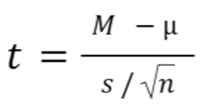
- M: Calculated mean of your sample
- μ: Hypothetical mean you are testing against
- s: The standard deviation of your sample
- n: The number of observations in your sample.
In a one-sample t test, calculating degrees of freedom is simple: one less than the number of objects in your dataset (you’ll see it written as n-1).
Example of a one sample t test
For our example within Prism, we have a dataset of 12 values from an experiment labeled “% of control”. Perhaps these are heights of a sample of plants that have been treated with a new fertilizer. A value of 100 represents the industry-standard control height. Likewise, 123 represents a plant with a height 123% that of the control (that is, 23% larger).
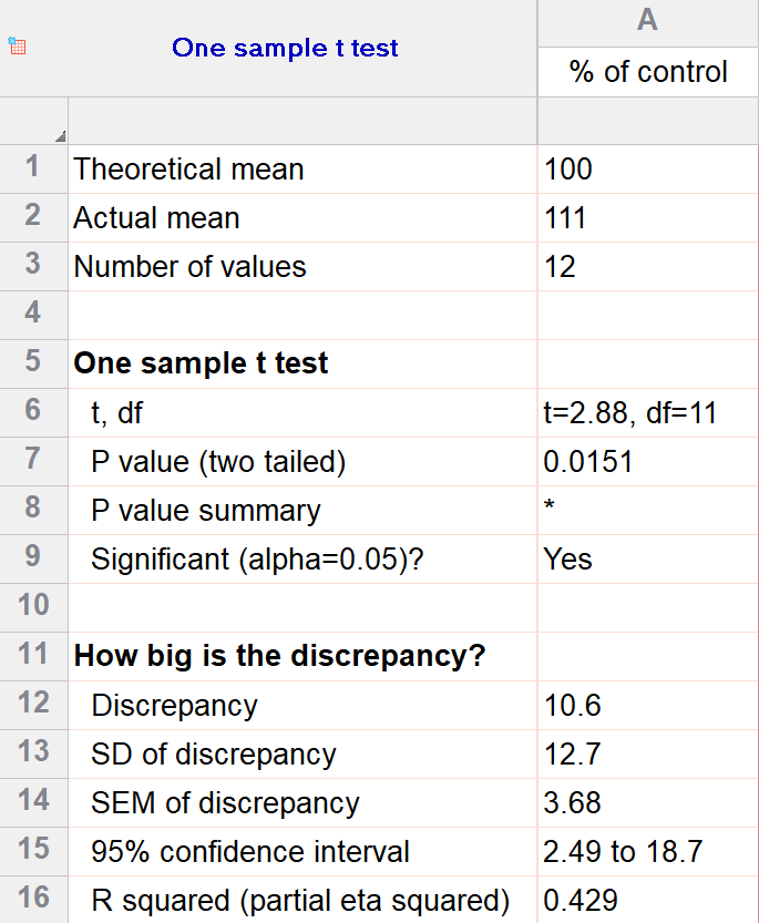
We’ll perform a two-tailed, one-sample t test to see if plants are shorter or taller on average with the fertilizer. We will use a significance threshold of 0.05. Here is the output:
You can see in the output that the actual sample mean was 111. Is that different enough from the industry standard (100) to conclude that there is a statistical difference?
The quick answer is yes, there’s strong evidence that the height of the plants with the fertilizer is greater than the industry standard (p=0.015). The nice thing about using software is that it handles some of the trickier steps for you. In this case, it calculates your test statistic (t=2.88), determines the appropriate degrees of freedom (11), and outputs a P value.
More informative than the P value is the confidence interval of the difference, which is 2.49 to 18.7. The confidence interval tells us that, based on our data, we are confident that the true difference between our sample and the baseline value of 100 is somewhere between 2.49 and 18.7. As long as the difference is statistically significant, the interval will not contain zero.
You can follow these tips for interpreting your own one-sample test.
Graphing a one-sample t test
For some techniques (like regression), graphing the data is a very helpful part of the analysis. For t tests, making a chart of your data is still useful to spot any strange patterns or outliers, but the small sample size means you may already be familiar with any strange things in your data.
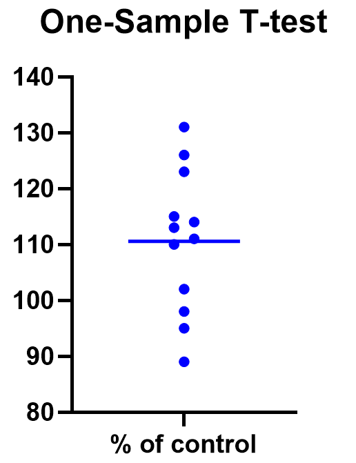
Here we have a simple plot of the data points, perhaps with a mark for the average. We’ve made this as an example, but the truth is that graphing is usually more visually telling for two-sample t tests than for just one sample.
Two sample t tests
There are several kinds of two sample t tests, with the two main categories being paired and unpaired (independent) samples.
Paired samples t test
In a paired samples t test, also called dependent samples t test, there are two samples of data, and each observation in one sample is “paired” with an observation in the second sample. The most common example is when measurements are taken on each subject before and after a treatment. A paired t test example research question is, “Is there a statistical difference between the average red blood cell counts before and after a treatment?”
Having two samples that are closely related simplifies the analysis. Statistical software, such as this paired t test calculator, will simply take a difference between the two values, and then compare that difference to 0.
In some (rare) situations, taking a difference between the pairs violates the assumptions of a t test, because the average difference changes based on the size of the before value (e.g., there’s a larger difference between before and after when there were more to start with). In this case, instead of using a difference test, use a ratio of the before and after values, which is referred to as ratio t tests.
Paired t test formula
The formula for paired samples t test is:
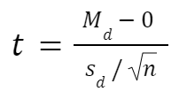
- Md: Mean difference between the samples
- sd: The standard deviation of the differences
- n: The number of differences
Degrees of freedom are the same as before. If you’re studying for an exam, you can remember that the degrees of freedom are still n-1 (not n-2) because we are converting the data into a single column of differences rather than considering the two groups independently.
Also note that the null value here is simply 0. There is no real reason to include “minus 0” in an equation other than to illustrate that we are still doing a hypothesis test. After you take the difference between the two means, you are comparing that difference to 0.
Example
For our example data, we have five test subjects and have taken two measurements from each: before (“control”) and after a treatment (“treated”). If we set alpha = 0.05 and perform a two-tailed test, we observe a statistically significant difference between the treated and control group (p=0.0160, t=4.01, df = 4). We are 95% confident that the true mean difference between the treated and control group is between 0.449 and 2.47.
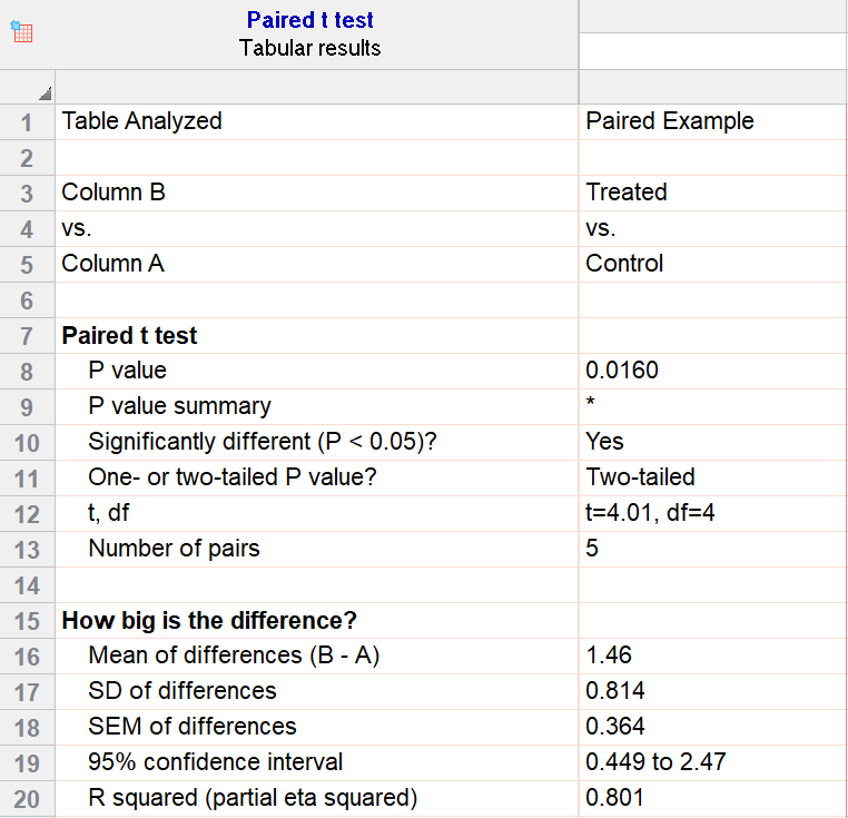
Graphing a paired t test
The significant result of the P value suggests evidence that the treatment had some effect, and we can also look at this graphically. The lines that connect the observations can help us spot a pattern, if it exists. In this case the lines show that all observations increased after treatment. While not all graphics are this straightforward, here it is very consistent with the outcome of the t test.
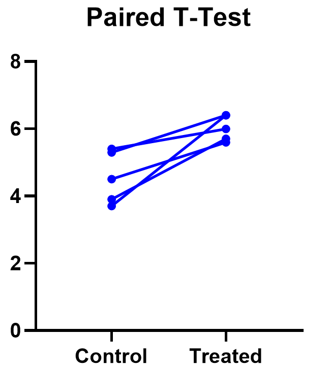
Prism’s estimation plot is even more helpful because it shows both the data (like above) and the confidence interval for the difference between means. You can easily see the evidence of significance since the confidence interval on the right does not contain zero.
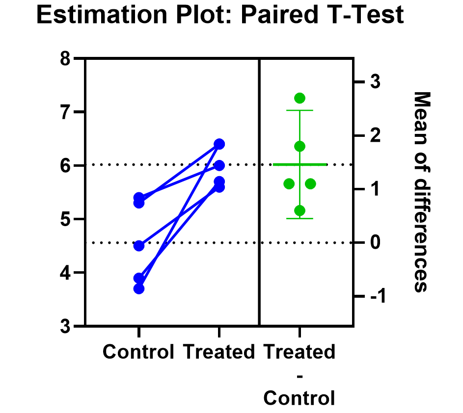
Here are some more graphing tips for paired t tests.
Unpaired samples t test
Unpaired samples t test, also called independent samples t test, is appropriate when you have two sample groups that aren’t correlated with one another. A pharma example is testing a treatment group against a control group of different subjects. Compare that with a paired sample, which might be recording the same subjects before and after a treatment.
With unpaired t tests, in addition to choosing your level of significance and a one or two tailed test, you need to determine whether or not to assume that the variances between the groups are the same or not. If you assume equal variances, then you can “pool” the calculation of the standard error between the two samples. Otherwise, the standard choice is Welch’s t test which corrects for unequal variances. This choice affects the calculation of the test statistic and the power of the test, which is the test’s sensitivity to detect statistical significance.
It’s best to choose whether or not you’ll use a pooled or unpooled (Welch’s) standard error before running your experiment, because the standard statistical test is notoriously problematic. See more details about unequal variances here.
As long as you’re using statistical software, such as this two-sample t test calculator, it’s just as easy to calculate a test statistic whether or not you assume that the variances of your two samples are the same. If you’re doing it by hand, however, the calculations get more complicated with unequal variances.
Unpaired (independent) samples t test formula
The general two-sample t test formula is:
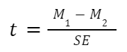
- M1 and M2: Two means you are comparing, one from each dataset
- SE: The combined standard error of the two samples (calculated using pooled or unpooled standard error)
The denominator (standard error) calculation can be complicated, as can the degrees of freedom. If the groups are not balanced (the same number of observations in each), you will need to account for both when determining n for the test as a whole.
Example
As an example for this family, we conduct a paired samples t test assuming equal variances (pooled). Based on our research hypothesis, we’ll conduct a two-tailed test, and use alpha=0.05 for our level of significance. Our samples were unbalanced, with two samples of 6 and 5 observations respectively.
The P value (p=0.261, t = 1.20, df = 9) is higher than our threshold of 0.05. We have not found sufficient evidence to suggest a significant difference. You can see the confidence interval of the difference of the means is -9.58 to 31.2.
Note that the F-test result shows that the variances of the two groups are not significantly different from each other.
Graphing an unpaired samples t test
For an unpaired samples t test, graphing the data can quickly help you get a handle on the two groups and how similar or different they are. Like the paired example, this helps confirm the evidence (or lack thereof) that is found by doing the t test itself.
Below you can see that the observed mean for females is higher than that for males. But because of the variability in the data, we can’t tell if the means are actually different or if the difference is just by chance.
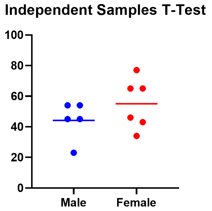
Nonparametric alternatives for t tests
If your data comes from a normal distribution (or something close enough to a normal distribution), then a t test is valid. If that assumption is violated, you can use nonparametric alternatives.
T tests evaluate whether the mean is different from another value, whereas nonparametric alternatives compare either the median or the rank. Medians are well-known to be much more robust to outliers than the mean.
The downside to nonparametric tests is that they don’t have as much statistical power, meaning a larger difference is required in order to determine that it’s statistically significant.
Wilcoxon signed-rank test
The Wilcoxon signed-rank test is the nonparametric cousin to the one-sample t test. This compares a sample median to a hypothetical median value. It is sometimes erroneously even called the Wilcoxon t test (even though it calculates a “W” statistic).
And if you have two related samples, you should use the Wilcoxon matched pairs test instead. The two versions of Wilcoxon are different, and the matched pairs version is specifically for comparing the median difference for paired samples.
Mann-Whitney and Kolmogorov-Smirnov tests
For unpaired (independent) samples, there are multiple options for nonparametric testing. Mann-Whitney is more popular and compares the mean ranks (the ordering of values from smallest to largest) of the two samples. Mann-Whitney is often misrepresented as a comparison of medians, but that’s not always the case. Kolmogorov-Smirnov tests if the overall distributions differ between the two samples.
More t test FAQs
What is the formula for a t test?
The exact formula depends on which type of t test you are running, although there is a basic structure that all t tests have in common. All t test statistics will have the form:
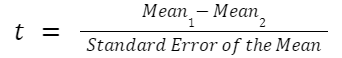
- t: The t test statistic you calculate for your test
- Mean1 and Mean2: Two means you are comparing, at least 1 from your own dataset
- Standard Error of the Mean: The standard error of the mean, also called the standard deviation of the mean, which takes into account the variance and size of your dataset
The exact formula for any t test can be slightly different, particularly the calculation of the standard error. Not only does it matter whether one or two samples are being compared, the relationship between the samples can make a difference too.
What is a t-distribution?
A t-distribution is similar to a normal distribution. It’s a bell-shaped curve, but compared to a normal it has fatter tails, which means that it’s more common to observe extremes. T-distributions are identified by the number of degrees of freedom. The higher the number, the closer the t-distribution gets to a normal distribution. After about 30 degrees of freedom, a t and a standard normal are practically the same.
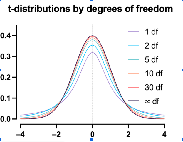 t-distribution by degree of freedom
What are degrees of freedom?
Degrees of freedom are a measure of how large your dataset is. They aren’t exactly the number of observations, because they also take into account the number of parameters (e.g., mean, variance) that you have estimated.
What is the difference between paired vs unpaired t tests?
Both paired and unpaired t tests involve two sample groups of data. With a paired t test, the values in each group are related (usually they are before and after values measured on the same test subject). In contrast, with unpaired t tests, the observed values aren’t related between groups. An unpaired, or independent t test, example is comparing the average height of children at school A vs school B.
When do I use a z-test versus a t test?
Z-tests, which compare data using a normal distribution rather than a t-distribution, are primarily used for two situations. The first is when you’re evaluating proportions (number of failures on an assembly line). The second is when your sample size is large enough (usually around 30) that you can use a normal approximation to evaluate the means.
When should I use ANOVA instead of a t test?
Use ANOVA if you have more than two group means to compare.
What are the differences between t test vs chi square?
Chi square tests are used to evaluate contingency tables, which record a count of the number of subjects that fall into particular categories (e.g., truck, SUV, car). t tests compare the mean(s) of a variable of interest (e.g., height, weight).
What are P values?
P values are the probability that you would get data as or more extreme than the observed data given that the null hypothesis is true. It’s a mouthful, and there are a lot of issues to be aware of with P values.
What are t test critical values?
Critical values are a classical form (they aren’t used directly with modern computing) of determining if a statistical test is significant or not. Historically you could calculate your test statistic from your data, and then use a t-table to look up the cutoff value (critical value) that represented a “significant” result. You would then compare your observed statistic against the critical value.
How do I calculate degrees of freedom for my t test?
In most practical usage, degrees of freedom are the number of observations you have minus the number of parameters you are trying to estimate. The calculation isn’t always straightforward and is approximated for some t tests.
Statistical software calculates degrees of freedom automatically as part of the analysis, so understanding them in more detail isn’t needed beyond assuaging any curiosity.
Perform your own t test
Are you ready to calculate your own t test? Start your 30 day free trial of Prism and get access to:
- A step by step guide on how to perform a t test
- Sample data to save you time
- More tips on how Prism can help your research
With Prism, in a matter of minutes you learn how to go from entering data to performing statistical analyses and generating high-quality graphs.