Extras: Steady-State Error
Contents
- Calculating steady-state errors
- System type and steady-state error
- Example: Meeting steady-state error requirements
Steady-state error is defined as the difference between the input (command) and the output of a system in the limit as time
goes to infinity (i.e. when the response has reached steady state). The steady-state error will depend on the type of input
(step, ramp, etc.) as well as the system type (0, I, or II).
Note: Steady-state error analysis is only useful for stable systems. You should always check the system for stability before
performing a steady-state error analysis. Many of the techniques that we present will give an answer even if the error does
not reach a finite steady-state value.
Calculating steady-state errors
Before talking about the relationships between steady-state error and system type, we will show how to calculate error regardless
of system type or input. Then, we will start deriving formulas we can apply when the system has a specific structure and the
input is one of our standard functions. Steady-state error can be calculated from the open- or closed-loop transfer function
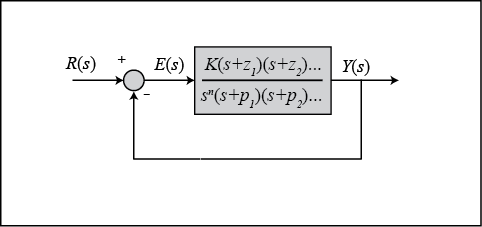
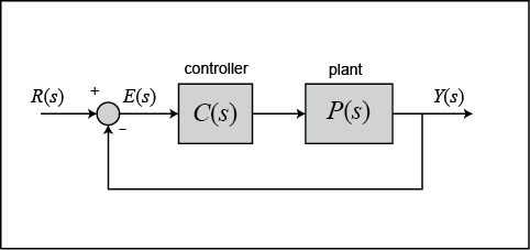
for unity feedback systems. For example, let’s say that we have the system given below.
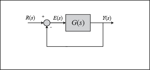
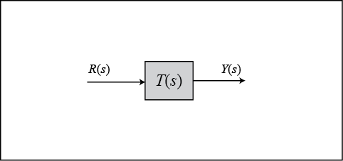
This is equivalent to the following system, where T(s) is the closed-loop transfer function.
We can calculate the steady-state error for this system from either the open- or closed-loop transfer function using the Final
Value Theorem. Recall that this theorem can only be applied if the subject of the limit (sE(s) in this case) has poles with negative real part.
(1)
(2)![$$ e(infty) = lim_{srightarrow0}sE(s) = lim_{srightarrow0}sR(s)[1-T(s)] $$](https://ctms.engin.umich.edu/CTMS/Content/Extras/html/Extras_Ess_eq05255288211822706456.png)
Now, let’s plug in the Laplace transforms for some standard inputs and determine equations to calculate steady-state error
from the open-loop transfer function in each case.
- Step Input (R(s) = 1 / s):
(3)
- Ramp Input (R(s) = 1 / s^2):
(4)
- Parabolic Input (R(s) = 1 / s^3):
(5)
When we design a controller, we usually also want to compensate for disturbances to a system. Let’s say that we have a system
with a disturbance that enters in the manner shown below.

We can find the steady-state error due to a step disturbance input again employing the Final Value Theorem (treat R(s) = 0).
(6)
When we have a non-unity feedback system we need to be careful since the signal entering G(s) is no longer the actual error E(s). Error is the difference between the commanded reference and the actual output, E(s) = R(s) — Y(s). When there is a transfer function H(s) in the feedback path, the signal being substracted from R(s) is no longer the true output Y(s), it has been distorted by H(s). This situation is depicted below.
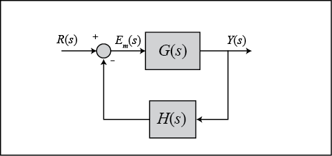
Manipulating the blocks, we can transform the system into an equivalent unity-feedback structure as shown below.
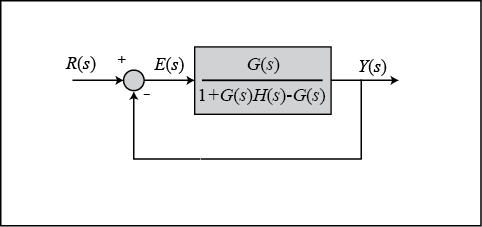
Then we can apply the equations we derived above.
System type and steady-state error
If you refer back to the equations for calculating steady-state errors for unity feedback systems, you will find that we have
defined certain constants (known as the static error constants). These constants are the position constant (Kp), the velocity constant (Kv), and the acceleration constant (Ka). Knowing the value of these constants, as well as the system type, we can predict if our system is going to have a finite
steady-state error.
First, let’s talk about system type. The system type is defined as the number of pure integrators in the forward path of a
unity-feedback system. That is, the system type is equal to the value of n when the system is represented as in the following figure. It does not matter if the integrators are part of the controller
or the plant.
Therefore, a system can be type 0, type 1, etc. The following tables summarize how steady-state error varies with system type.
| Type 0 system | Step Input | Ramp Input | Parabolic Input |
|---|---|---|---|
| Steady-State Error Formula | 1/(1+Kp) | 1/Kv | 1/Ka |
| Static Error Constant | Kp = constant | Kv = 0 | Ka = 0 |
| Error | 1/(1+Kp) | infinity | infinity |
| Type 1 system | Step Input | Ramp Input | Parabolic Input |
|---|---|---|---|
| Steady-State Error Formula | 1/(1+Kp) | 1/Kv | 1/Ka |
| Static Error Constant | Kp = infinity | Kv = constant | Ka = 0 |
| Error | 0 | 1/Kv | infinity |
| Type 2 system | Step Input | Ramp Input | Parabolic Input |
|---|---|---|---|
| Steady-State Error Formula | 1/(1+Kp) | 1/Kv | 1/Ka |
| Static Error Constant | Kp = infinity | Kv = infinity | Ka = constant |
| Error | 0 | 0 | 1/Ka |
Example: Meeting steady-state error requirements
Consider a system of the form shown below.
For this example, let G(s) equal the following.
(7)
Since this system is type 1, there will be no steady-state error for a step input and there will be infinite error for a parabolic
input. The only input that will yield a finite steady-state error in this system is a ramp input. We wish to choose K such that the closed-loop system has a steady-state error of 0.1 in response to a ramp reference. Let’s first examine the
ramp input response for a gain of K = 1.
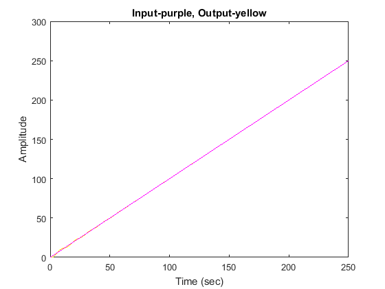
s = tf('s');
G = ((s+3)*(s+5))/(s*(s+7)*(s+8));
T = feedback(G,1);
t = 0:0.1:25;
u = t;
[y,t,x] = lsim(T,u,t);
plot(t,y,'y',t,u,'m')
xlabel('Time (sec)')
ylabel('Amplitude')
title('Input-purple, Output-yellow')
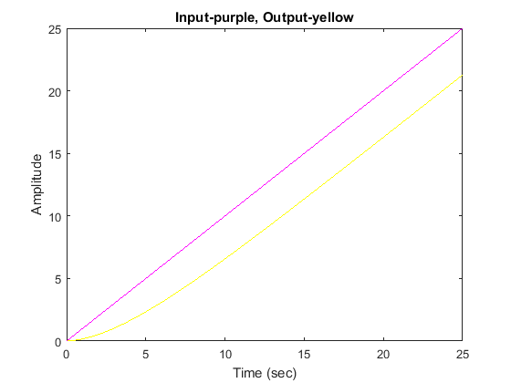
The steady-state error for this system is quite large, since we can see that at time 20 seconds the output is approximately
16 as compared to an input of 20 (steady-state error is approximately equal to 4). Let’s examine this in further detail.
We know from our problem statement that the steady-state error must be 0.1. Therefore, we can solve the problem following
these steps:
(8)
(9)
(10)
Let’s see the ramp input response for K = 37.33 by entering the following code in the MATLAB command window.
K = 37.33 ;
s = tf('s');
G = (K*(s+3)*(s+5))/(s*(s+7)*(s+8));
sysCL = feedback(G,1);
t = 0:0.1:50;
u = t;
[y,t,x] = lsim(sysCL,u,t);
plot(t,y,'y',t,u,'m')
xlabel('Time (sec)')
ylabel('Amplitude')
title('Input-purple, Output-yellow')
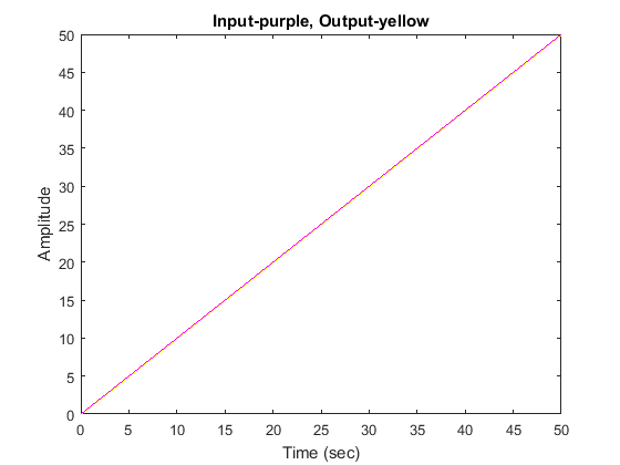
In order to get a better view, we must zoom in on the response. We choose to zoom in between time equals 39.9 and 40.1 seconds
because that will ensure that the system has reached steady state.
axis([39.9,40.1,39.9,40.1])
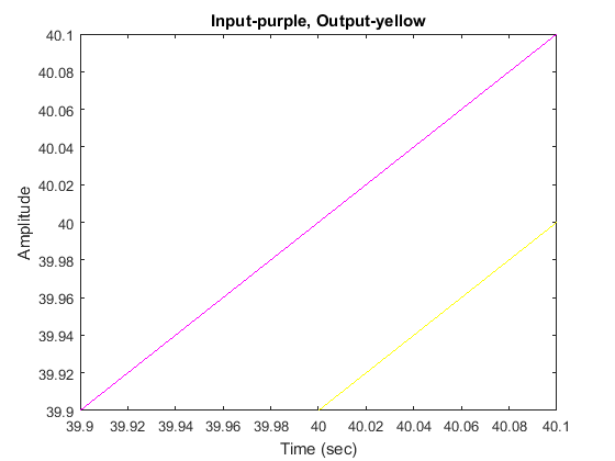
Examination of the above shows that the steady-state error is indeed 0.1 as desired.
Now let’s modify the problem a little bit and say that our system has the form shown below.
In essence we are not distinguishing between the controller and the plant in our feedback system. Now we want to achieve zero
steady-state error for a ramp input.
From our tables, we know that a system of type 2 gives us zero steady-state error for a ramp input. Therefore, we can get
zero steady-state error by simply adding an integrator (a pole at the origin). Let’s view the ramp input response for a step
input if we add an integrator and employ a gain K = 1.
s = tf('s');
P = ((s+3)*(s+5))/(s*(s+7)*(s+8));
C = 1/s;
sysCL = feedback(C*P,1);
t = 0:0.1:250;
u = t;
[y,t,x] = lsim(sysCL,u,t);
plot(t,y,'y',t,u,'m')
xlabel('Time (sec)')
ylabel('Amplitude')
title('Input-purple, Output-yellow')
As you can see, there is initially some oscillation (you may need to zoom in). However, at steady state we do have zero steady-state
error as desired. Let’s zoom in around 240 seconds (trust me, it doesn’t reach steady state until then).
axis([239.9,240.1,239.9,240.1])
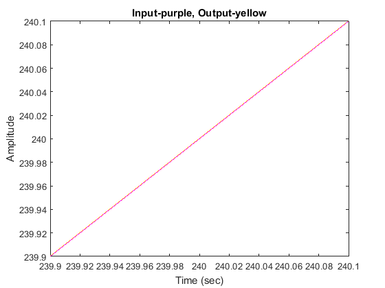
As you can see, the steady-state error is zero. Feel free to zoom in on different areas of the graph to observe how the response
approaches steady state.
The deviation of the output of control system from desired response during steady state is known as steady state error. It is represented as $e_{ss}$. We can find steady state error using the final value theorem as follows.
$$e_{ss}=lim_{t to infty}e(t)=lim_{s to 0}sE(s)$$
Where,
E(s) is the Laplace transform of the error signal, $e(t)$
Let us discuss how to find steady state errors for unity feedback and non-unity feedback control systems one by one.
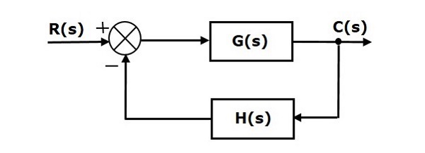
Steady State Errors for Unity Feedback Systems
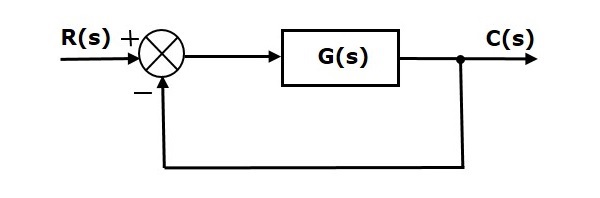
Consider the following block diagram of closed loop control system, which is having unity negative feedback.
Where,
- R(s) is the Laplace transform of the reference Input signal $r(t)$
- C(s) is the Laplace transform of the output signal $c(t)$
We know the transfer function of the unity negative feedback closed loop control system as
$$frac{C(s)}{R(s)}=frac{G(s)}{1+G(s)}$$
$$Rightarrow C(s)=frac{R(s)G(s)}{1+G(s)}$$
The output of the summing point is —
$$E(s)=R(s)-C(s)$$
Substitute $C(s)$ value in the above equation.
$$E(s)=R(s)-frac{R(s)G(s)}{1+G(s)}$$
$$Rightarrow E(s)=frac{R(s)+R(s)G(s)-R(s)G(s)}{1+G(s)}$$
$$Rightarrow E(s)=frac{R(s)}{1+G(s)}$$
Substitute $E(s)$ value in the steady state error formula
$$e_{ss}=lim_{s to 0} frac{sR(s)}{1+G(s)}$$
The following table shows the steady state errors and the error constants for standard input signals like unit step, unit ramp & unit parabolic signals.
| Input signal | Steady state error $e_{ss}$ | Error constant |
|---|---|---|
|
unit step signal |
$frac{1}{1+k_p}$ |
$K_p=lim_{s to 0}G(s)$ |
|
unit ramp signal |
$frac{1}{K_v}$ |
$K_v=lim_{s to 0}sG(s)$ |
|
unit parabolic signal |
$frac{1}{K_a}$ |
$K_a=lim_{s to 0}s^2G(s)$ |
Where, $K_p$, $K_v$ and $K_a$ are position error constant, velocity error constant and acceleration error constant respectively.
Note − If any of the above input signals has the amplitude other than unity, then multiply corresponding steady state error with that amplitude.
Note − We can’t define the steady state error for the unit impulse signal because, it exists only at origin. So, we can’t compare the impulse response with the unit impulse input as t denotes infinity.
Example
Let us find the steady state error for an input signal $r(t)=left( 5+2t+frac{t^2}{2} right )u(t)$ of unity negative
feedback control system with $G(s)=frac{5(s+4)}{s^2(s+1)(s+20)}$
The given input signal is a combination of three signals step, ramp and parabolic. The following table shows the error constants and steady state error values for these three signals.
| Input signal | Error constant | Steady state error |
|---|---|---|
|
$r_1(t)=5u(t)$ |
$K_p=lim_{s to 0}G(s)=infty$ |
$e_{ss1}=frac{5}{1+k_p}=0$ |
|
$r_2(t)=2tu(t)$ |
$K_v=lim_{s to 0}sG(s)=infty$ |
$e_{ss2}=frac{2}{K_v}=0$ |
|
$r_3(t)=frac{t^2}{2}u(t)$ |
$K_a=lim_{s to 0}s^2G(s)=1$ |
$e_{ss3}=frac{1}{k_a}=1$ |
We will get the overall steady state error, by adding the above three steady state errors.
$$e_{ss}=e_{ss1}+e_{ss2}+e_{ss3}$$
$$Rightarrow e_{ss}=0+0+1=1$$
Therefore, we got the steady state error $e_{ss}$ as 1 for this example.
Steady State Errors for Non-Unity Feedback Systems
Consider the following block diagram of closed loop control system, which is having nonunity negative feedback.
We can find the steady state errors only for the unity feedback systems. So, we have to convert the non-unity feedback system into unity feedback system. For this, include one unity positive feedback path and one unity negative feedback path in the above block diagram. The new block diagram looks like as shown below.
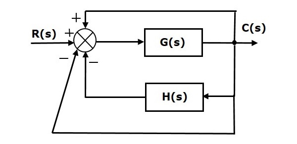
Simplify the above block diagram by keeping the unity negative feedback as it is. The following is the simplified block diagram.
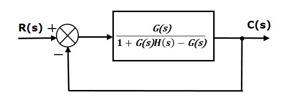
This block diagram resembles the block diagram of the unity negative feedback closed loop control system. Here, the single block is having the transfer function $frac{G(s)}{1+G(s)H(s)-G(s)}$ instead of $G(s)$. You can now calculate the steady state errors by using steady state error formula given for the unity negative feedback systems.
Note − It is meaningless to find the steady state errors for unstable closed loop systems. So, we have to calculate the steady state errors only for closed loop stable systems. This means we need to check whether the control system is stable or not before finding the steady state errors. In the next chapter, we will discuss the concepts-related stability.
In this post I want to talk about the Final Value Theorem and steady state error because these concepts will be useful as we go on to discuss controller design in more detail. Steady state error describes how far the system deviates from the desired reference signal as time goes to infinity [1]. It is a commonly used performance metric for controller design, which is why I want to establish the concept now before we apply it in future posts on controller design [2]. I will start the discussion, though, with the Final Value Theorem because that concept is critical to understanding steady state error.
The Final Value Theorem is used to find the “final value” of a system as time goes to infinity. It is derived from the Laplace transform of the derivative, taken as time goes to infinity (or s goes to zero), as shown in the equation below [2]. Note that we can only use the Final Value Theorem if a system is stable, or at least has all its poles at the origin (and the left half plane). If the system is unstable or a non-decaying sinusoid, then the Final Value Theorem will produce results, but they will be meaningless because the system does not actually converge to zero [1],[2]. Don’t be fooled — always test for stability before using the Final Value Theorem!

Now that we have the Final Value Theorem equation, we can use it to find the steady state error. The formal definition of steady state error, according to Nise, is the difference between a reference signal and the corresponding output signal for a prescribed test input as time goes to infinity [2]. I italicized “for a prescribed test input” because this helps to understand the process we are going to use. We are going to take the transfer function of the error of a system and apply a test input to that transfer function. The test input can be a step input (corresponds to a position command), a ramp input (corresponds to a velocity command) or a parabolic input (corresponds to an acceleration command) [1], [2]. The error transfer function will describe how the system error responds to that input, and we can use the Final Value Theorem to see how the error will respond in the long-term. This is shown in Equation 2 below.

Note that for unity feedback, you can also write the error as the ratio between the reference signal and the forward transfer function, G(s) [2]. This is shown in Equation 3 below. This form will be helpful in the next step of our discussion.

If we substitute the test input for R(s) and solve the Final Value Theorem for our system, we can get 3 possible types of steady state errors:
(1) Zero error: this means that the system is capable of eliminating all steady state error. In order to do this the system must have at least one pole at the origin (an integrator).
(2) Finite error: this means that the system is capable of reaching steady state given this input, but it does not have enough integrators to eliminate all of the error produced by following the test signal.
(3) Infinite error: this means that the system cannot track this reference signal at all.
The results of the steady state error equation can also be used to help us determine the system “Type”. The system type is a number corresponding to the number of integrators it possesses [1]. For example, if a system is Type 0, it does not have any integrators. It can only track a step input, but even with that input it will have some finite steady state error because it has no integrators with which to eliminate that error. Conversely, a Type 1 system has 1 integrator and it can track a step input with zero error and a ramp input with finite error [1], [2].
What if you want to find the steady state error contribution from a disturbance input? I have shown the block diagram for a disturbance input and the derivation of the equation for steady state error in the figure below. Notice that I went back to the fundamentals shown in Equation 1 to get the equation for steady state error as a function of contributions from both the reference signal and the disturbance signal.

Figure 1
We also made an important assumption in our discussion up to this point: we assumed that we had unity feedback because it simplified the math. However, we often have non-unity feedback because sensor noise and system dynamics can contribute to the feedback path of our system. In these cases, it is helpful to apply the trick demonstrated below to re-draw the block diagram as a unity feedback system. I have worked out some of the math alongside the diagrams.

Figure 2
Now that we have this concept in hand, next time we will work through an example of the design process to meet steady state and transient performance requirements using root locus plots.
References
[1] Douglas, Brian. “Final Value Theorem and Steady State Error.” https://www.youtube.com/watch?v=PXxveGoNRUw&list=PLUMWjy5jgHK1NC52DXXrriwihVrYZKqjk&index=15 Viewed on 07/23/2019.
[2] Nise, Norman S. Control Systems Engineering, 4th Ed. John Wiley & Sons, Inc. 2004.
Errors in a control system can be attributed to many factors. Changes in the reference input will cause unavoidable errors during transient periods and may also cause steady-state errors. Imperfections in the system components, such as static friction, backlash, and amplifier drift, as well as aging or deterioration, will cause errors at steady state. In this section, however, we shall not discuss errors due to imperfections in the system components. Rather, we shall investigate a type of steady-state error that is caused by the incapability of a system to follow particular types of inputs.
Steady-state error is the difference between the input and the output for a prescribed test input as time tends to infinity. Test inputs used for steady-state error analysis and design are summarized in Table 7.1. In order to explain how these test signals are used, let us assume a position control system, where the output position follows the input commanded position.

Step inputs represent constant position and thus are useful in determining the ability of the control system to position itself with respect to a stationary target. An antenna position control is an example of a system that can be tested for accuracy using step inputs.
Ramp inputs represent constant-velocity inputs to a position control system by their linearly increasing amplitude. These waveforms can be used to test a system’s ability to follow a linearly increasing input or, equivalently, to track a constant velocity target. For example, a position control system that tracks a satellite that moves across the sky at a constant angular velocity.
Parabolas inputs, whose second derivatives are constant, represent constant acceleration inputs to position control systems and can be used to represent accelerating targets, such as a missile.
Any physical control system inherently suffers steady-state error in response to certain types of inputs. A system may have no steady-state error to a step input, but the same system may exhibit nonzero steady-state error to a ramp input. (The only way we may be able to eliminate this error is to modify the system structure.) Whether a given system will exhibit steady-state error for a given type of input depends on the type of open-loop transfer function of the system.
Definition of the error in steady state depending on the configuration of the system.
The steady-state errors of linear control systems depend on the type of the reference signal and the type of system. Before undertaking the error in steady state, it must be clarified what is the meaning of the system error.
The error can be seen as a signal that should quickly be reduced to zero, if this is possible. Consider the system of Figure 7-5:


Where r (t) is the input signal, u (t) is the acting signal, b (t) is the feedback signal and y (t) is the output signal. The error e (t) of the system can be defined as:

We must remember that r (t) and y (t) do not necessarily have the same dimensions. On the other hand, when the system has unit feedback, H (s) = 1, the input r (t) is the reference signal and the error is simply:

That is, the error is the acting signal, u (t). When H (s) is not equal to 1, u (t) may or may not be the error, depending on the form and purpose of H (s). Therefore, the reference signal must be defined when H (s) is not equal to 1.
The error in steady state is defined as:

To establish a systematic study of the error in steady state for linear systems, we will classify the control systems as follows:
- Unit feedback systems,
- Non-unit feedback systems.
Steady-State Error in Unity-feedback control systems
Consider the system shown in Figure 5-49:

The closed-loop transfer function for this can be obtained as:

The transfer function between the error signal e(t) and the input signal r(t) is:

Where the error e(t) is the difference between the input signal and the output signal. The final-value theorem provides a convenient way to find the steady-state performance of a stable system. Since:

The steady-state error is:

This last equation allows us to calculate the steady-state error Ess, given the input R(s) and the transfer function G(s). We then substitute several inputs for R(s) and then draw conclusions about the relationship that exists between the open-loop system G(s) and the nature of the steady-state error Ess.
- Step Input: Using R(s) =1/S, we obtain:

Where:

Is the gain of the forward transfer function. In order to have zero steady-state error,

To satisfy the last condition, G(s) must have the following form:

And for the limit to be infinite the denominator must be equal to zero a S goes to zero. So n>=1, that is, at least one pole must be at the origin, equal to say that at least one pure integration must be present in the forward path. The steady-state respond for this case of zero steady-state error is similar to that shown in Figure 7-2a, ouput 1.


If there are no integrations, the n=0, and it yields a finite error. This is the case shown in Figure 7-2a, output 2.
In summary, for a step input to a unity feedback system, the steady-state error will be zero if there is at least one pure integration in the forward path.
- Ramp Input: Using R(s) =1/Sˆ2, we obtain:

To have zero steady-state error to a ramp input we must have:

To satisfy this G(s) must take the form where n>=2. In other words, there must be at least two integrations in the forward path. An example of a steady-state error for a ramp input is shown in Figure 7.2b, output 1:


If only one integrator exist in the forward path then lim sG(s) is finite rather tan infinite and this lead to a constant error, as shown in Figure 7.2b, output 2. If there is only one integrator in the forward path then lim sG(s) =0, and the steady-state error will be infinite and lead to diverging ramp, as shown in Figure 7.2b, output 3.
- Parabolic Input: Using R(s) =1/Sˆ3, we obtain:

In order to have zero steady-state error for a parabolic input, we must have:

To satisfy this G(s) n must be n>=3. In other words, there must be at least three integrations in the forward path. If there only two integrators in the forward path then lim sˆ2G(s) is finite rather tan infinite and this lead to a constant error. If there one or zero integrators in the forward path then e() is infinite.
Classification of Control Systems (System Types) and Static Errors Constant.
System Type. Control system may be classified according to their ability to follow step inputs, ramp inputs or parabolic inputs and so on. This is a reasonable classification scheme because most of the actual inputs can be considered a combination of such inputs. Consider the unity-feedback control system with the following open-loop transfer function G(s):

It involves the term SˆN in the denominator, representing a pole of multiplicity N at the origin. A system is called type 0, type 1, type 2,…if N=0, 1, 2…respectively. As the type increases, accuracy is improved. However, this agraves the stability problem. If G(s) is written so that each term in the numerator and denominator, except the term SˆN, approaches unity as s approaches zero, then the open-loop gain K is directly related to the steady-state error.
Static Error Constant. The Static Error Constants defined in the following are figures of merit of control systems. The higher the constants, the smaller the steady-state error.
- Static Position Error Constant Kp. The steady-state error of a system for a unit-step input is:

The Static Position Error Constant Kp is defined by:

Thus the steady-state error in terms of the Static Position Error Constant Kp is given by:

For a type 0 system:

For a type 1 or higher system:

- Static Velocity Error Constant Kv. The steady-state error of a system for a unit-ramp input is given by:

The Static Velocity Error Constant Kv is defined by:

Thus the steady-state error in terms of the Static Velocity Error Constant Kv is given by:

For a type 0 system:

For a type 1 system:

For For a type 2 system or higher:

- Static Acceleration Error Constant Ka. The steady-state error of a system for a unit-parabolic input is given by:

The Static Acceleration Error Constant Kv is defined by:

Thus the steady-state error in terms of the Static Acceleration Error Constant Ka is given by:

For a type 0 system:

For a type 1 system:

For a type 2 system:

For a type 3 system or higher:

Table 7.2 ties together the concepts of steady-state error, static error constants and system type. The table shows the static error constants and the steady-state error as a functions of the input waveform and the system type.

Steady-State Error for Non-unity Feedback Systems.
Control systems often do not have unity feedback because of the compensation used to improve performance or because of the physical model of the system. In these cases the most practical way to analyze the steady-state error is to take the system and form a unity feedback system by adding and subtracting unity feedback paths as shown in Figure 7.15:


Donde G(s)=G1(s)G2(s) y H(s)=H1(s)/G1(s). Notice that these steps require that input and output signals have the same units.
BEFORE: Control System Stability
NEXT: PID -Basic control system actions
Sources:
- Control Systems Engineering, Nise pp 340, 353
- Sistemas de Control Automatico Benjamin C Kuo pp 390, 395
- Modern_Control_Engineering, Ogata 4t pp 301,305
Written by: Larry Francis Obando – Technical Specialist – Educational Content Writer.
- WhatsApp: +34 633129287
- dademuchconnection@gmail.com
I resolve problems and exercises in two hours …Inmediate attention!!..
Escuela de Ingeniería Eléctrica de la Universidad Central de Venezuela, Caracas.
Escuela de Ingeniería Electrónica de la Universidad Simón Bolívar, Valle de Sartenejas.
Escuela de Turismo de la Universidad Simón Bolívar, Núcleo Litoral.
Contact: Jaén – España: Tlf. 633129287
Caracas, Quito, Guayaquil, Lima, México, Bogotá, Cochabamba, Santiago.
WhatsApp: +34 633129287
FACEBOOK: DademuchConnection
email: dademuchconnection@gmail.com
Attention: If what you need to solve urgently a problem of a “Mass-Spring-Damper System ” (find the output X (t), graphs in Matlab of the 2nd Order system and relevant parameters, etc.), or a “System of Electromechanical Control “… or simply need an advisor to solve the problem and study for the next test… send the problem…I Will Write The Solution …
Related:
The Block Diagram – Control Engineering
Dinámica de un Sistema Masa-Resorte-Amortiguador
Block Diagram of Electromechanical Systems – DC Motor
Transient-response Specifications
Control System Stability