Sum of squares of error - Исправление ошибок и поиск оптимальных решений проблем

From Wikipedia, the free encyclopedia

In statistics, the residual sum of squares (RSS), also known as the sum of squared estimate of errors (SSE), is the sum of the squares of residuals (deviations predicted from actual empirical values of data). It is a measure of the discrepancy between the data and an estimation model, such as a linear regression. A small RSS indicates a tight fit of the model to the data. It is used as an optimality criterion in parameter selection and model selection.

In general, total sum of squares = explained sum of squares + residual sum of squares. For a proof of this in the multivariate ordinary least squares (OLS) case, see partitioning in the general OLS model.

One explanatory variable[edit]

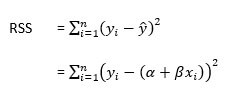
In a model with a single explanatory variable, RSS is given by:^[1]

${displaystyle operatorname {RSS} =sum _{i=1}^{n}(y_{i}-f(x_{i}))^{2}}$

where y_i is the i^th value of the variable to be predicted, x_i is the i^th value of the explanatory variable, and $f(x_{i})$ is the predicted value of y_i (also termed ${hat {y_{i}}}$ ).
In a standard linear simple regression model, ${displaystyle y_{i}=alpha +beta x_{i}+varepsilon _{i},}$ , where alpha and beta are coefficients, y and x are the regressand and the regressor, respectively, and ε is the error term. The sum of squares of residuals is the sum of squares of ${displaystyle {widehat {varepsilon ,}}_{i}}$ ; that is

${displaystyle operatorname {RSS} =sum _{i=1}^{n}({widehat {varepsilon ,}}_{i})^{2}=sum _{i=1}^{n}(y_{i}-({widehat {alpha ,}}+{widehat {beta ,}}x_{i}))^{2}}$

where is the estimated value of the constant term alpha and is the estimated value of the slope coefficient beta .

Matrix expression for the OLS residual sum of squares[edit]

The general regression model with n observations and k explanators, the first of which is a constant unit vector whose coefficient is the regression intercept, is

where y is an n × 1 vector of dependent variable observations, each column of the n × k matrix X is a vector of observations on one of the k explanators, beta is a k × 1 vector of true coefficients, and e is an n× 1 vector of the true underlying errors. The ordinary least squares estimator for beta is

${displaystyle X^{operatorname {T} }X{hat {beta }}=X^{operatorname {T} }yiff }$

${displaystyle {hat {beta }}=(X^{operatorname {T} }X)^{-1}X^{operatorname {T} }y.}$

The residual vector ${displaystyle {hat {e}}=y-X{hat {beta }}=y-X(X^{operatorname {T} }X)^{-1}X^{operatorname {T} }y}$ ; so the residual sum of squares is:

${displaystyle operatorname {RSS} ={hat {e}}^{operatorname {T} }{hat {e}}=|{hat {e}}|^{2}}$

(equivalent to the square of the norm of residuals). In full:

${displaystyle operatorname {RSS} =y^{operatorname {T} }y-y^{operatorname {T} }X(X^{operatorname {T} }X)^{-1}X^{operatorname {T} }y=y^{operatorname {T} }[I-X(X^{operatorname {T} }X)^{-1}X^{operatorname {T} }]y=y^{operatorname {T} }[I-H]y}$

where H is the hat matrix, or the projection matrix in linear regression.

Relation with Pearson’s product-moment correlation[edit]

The least-squares regression line is given by

where and ${displaystyle a={frac {S_{xy}}{S_{xx}}}}$ , where ${displaystyle S_{xy}=sum _{i=1}^{n}({bar {x}}-x_{i})({bar {y}}-y_{i})}$ and ${displaystyle S_{xx}=sum _{i=1}^{n}({bar {x}}-x_{i})^{2}.}$

Therefore,

${displaystyle {begin{aligned}operatorname {RSS} &=sum _{i=1}^{n}(y_{i}-f(x_{i}))^{2}=sum _{i=1}^{n}(y_{i}-(ax_{i}+b))^{2}=sum _{i=1}^{n}(y_{i}-ax_{i}-{bar {y}}+a{bar {x}})^{2}\[5pt]&=sum _{i=1}^{n}(a({bar {x}}-x_{i})-({bar {y}}-y_{i}))^{2}=a^{2}S_{xx}-2aS_{xy}+S_{yy}=S_{yy}-aS_{xy}=S_{yy}left(1-{frac {S_{xy}^{2}}{S_{xx}S_{yy}}}right)end{aligned}}}$

where ${displaystyle S_{yy}=sum _{i=1}^{n}({bar {y}}-y_{i})^{2}.}$

The Pearson product-moment correlation is given by ${displaystyle r={frac {S_{xy}}{sqrt {S_{xx}S_{yy}}}};}$ therefore, ${displaystyle operatorname {RSS} =S_{yy}(1-r^{2}).}$

References[edit]

^ Archdeacon, Thomas J. (1994). Correlation and regression analysis : a historian’s guide. University of Wisconsin Press. pp. 161–162. ISBN 0-299-13650-7. OCLC 27266095.

Draper, N.R.; Smith, H. (1998). Applied Regression Analysis (3rd ed.). John Wiley. ISBN 0-471-17082-8.

Источник

Download Article

The sum of squared errors, or SSE, is a preliminary statistical calculation that leads to other data values. When you have a set of data values, it is useful to be able to find how closely related those values are. You need to get your data organized in a table, and then perform some fairly simple calculations. Once you find the SSE for a data set, you can then go on to find the variance and standard deviation.

1

Create a three column table. The clearest way to calculate the sum of squared errors is begin with a three column table. Label the three columns as , , and ${text{Deviation}}^{2}$ .^[1]
2
Fill in the data. The first column will hold the values of your measurements. Fill in the column with the values of your measurements. These may be the results of some experiment, a statistical study, or just data provided for a math problem.^[2]
- In this case, suppose you are working with some medical data and you have a list of the body temperatures of ten patients. The normal body temperature expected is 98.6 degrees. The temperatures of ten patients are measured and give the values 99.0, 98.6, 98.5, 101.1, 98.3, 98.6, 97.9, 98.4, 99.2, and 99.1. Write these values in the first column.
Advertisement
3

Calculate the mean. Before you can calculate the error for each measurement, you must calculate the mean of the full data set.^[3]
4
Calculate the individual error measurements. In the second column of your table, you need to fill in the error measurements for each data value. The error is the difference between the measurement and the mean.^[4]
- For the given data set, subtract the mean, 98.87, from each measured value, and fill in the second column with the results. These ten calculations are as follows:
5
Calculate the squares of the errors. In the third column of the table, find the square of each of the resulting values in the middle column. These represent the squares of the deviation from the mean for each measured value of data.^[5]
- For each value in the middle column, use your calculator and find the square. Record the results in the third column, as follows:
6
Add the squares of errors together. The final step is to find the sum of the values in the third column. The desired result is the SSE, or the sum of squared errors.^[6]
- For this data set, the SSE is calculated by adding together the ten values in the third column:

1
Label the columns of the spreadsheet. You will create a three column table in Excel, with the same three headings as above.
- In cell A1, type in the heading “Value.”
- In cell B1, enter the heading “Deviation.»
- In cell C1, enter the heading “Deviation squared.”
2

Enter your data. In the first column, you need to type in the values of your measurements. If the set is small, you can simply type them in by hand. If you have a large data set, you may need to copy and paste the data into the column.
3
Find the mean of the data points. Excel has a function that will calculate the mean for you. In some vacant cell underneath your data table (it really doesn’t matter what cell you choose), enter the following:^[7]
- =Average(A2:___)
- Do not actually type a blank space. Fill in that blank with the cell name of your last data point. For example, if you have 100 points of data, you will use the function:
  - =Average(A2:A101)
  - This function includes data from A2 through A101 because the top row contains the headings of the columns.
- When you press Enter or when you click away to any other cell on the table, the mean of your data values will automatically fill the cell that you just programmed.
4
Enter the function for the error measurements. In the first empty cell in the “Deviation” column, you need to enter a function to calculate the difference between each data point and the mean. To do this, you need to use the cell name where the mean resides. Let’s assume for now that you used cell A104.^[8]
- The function for the error calculation, which you enter into cell B2, will be:
  - =A2-$A$104. The dollar signs are necessary to make sure that you lock in cell A104 for each calculation.
5
Enter the function for the error squares. In the third column, you can direct Excel to calculate the square that you need.^[9]
- In cell C2, enter the function
  - =B2^2
6
Copy the functions to fill the entire table. After you have entered the functions in the top cell of each column, B2 and C2 respectively, you need to fill in the full table. You could retype the function in every line of the table, but this would take far too long. Use your mouse, highlight cells B2 and C2 together, and without letting go of the mouse button, drag down to the bottom cell of each column.
- If we are assuming that you have 100 data points in your table, you will drag your mouse down to cells B101 and C101.
- When you then release the mouse button, the formulas will be copied into all the cells of the table. The table should be automatically populated with the calculated values.
7
Find the SSE. Column C of your table contains all the square-error values. The final step is to have Excel calculate the sum of these values.^[10]
- In a cell below the table, probably C102 for this example, enter the function:
  - =Sum(C2:C101)
- When you click Enter or click away into any other cell of the table, you should have the SSE value for your data.

1
Calculate variance from SSE. Finding the SSE for a data set is generally a building block to finding other, more useful, values. The first of these is variance. The variance is a measurement that indicates how much the measured data varies from the mean. It is actually the average of the squared differences from the mean.^[11]
- Because the SSE is the sum of the squared errors, you can find the average (which is the variance), just by dividing by the number of values. However, if you are calculating the variance of a sample set, rather than a full population, you will divide by (n-1) instead of n. Thus:
  - Variance = SSE/n, if you are calculating the variance of a full population.
  - Variance = SSE/(n-1), if you are calculating the variance of a sample set of data.
- For the sample problem of the patients’ temperatures, we can assume that 10 patients represent only a sample set. Therefore, the variance would be calculated as:
2
Calculate standard deviation from SSE. The standard deviation is a commonly used value that indicates how much the values of any data set deviate from the mean. The standard deviation is the square root of the variance. Recall that the variance is the average of the square error measurements.^[12]
- Therefore, after you calculate the SSE, you can find the standard deviation as follows:
  - ${text{Standard Deviation}}={sqrt {{frac {{text{SSE}}}{n-1}}}}$
- For the data sample of the temperature measurements, you can find the standard deviation as follows:
3
Use SSE to measure covariance. This article has focused on data sets that measure only a single value at a time. However, in many studies, you may be comparing two separate values. You would want to know how those two values relate to each other, not only to the mean of the data set. This value is the covariance.^[13]
- The calculations for covariance are too involved to detail here, other than to note that you will use the SSE for each data type and then compare them. For a more detailed description of covariance and the calculations involved, see Calculate Covariance.
- As an example of the use of covariance, you might want to compare the ages of the patients in a medical study to the effectiveness of a drug in lowering fever temperatures. Then you would have one data set of ages and a second data set of temperatures. You would find the SSE for each data set, and then from there find the variance, standard deviations and covariance.

Ask a Question

200 characters left

Include your email address to get a message when this question is answered.

Submit

Thanks for submitting a tip for review!

References

About This Article

Article SummaryX

To calculate the sum of squares for error, start by finding the mean of the data set by adding all of the values together and dividing by the total number of values. Then, subtract the mean from each value to find the deviation for each value. Next, square the deviation for each value. Finally, add all of the squared deviations together to get the sum of squares for error. To learn how to calculate the sum of squares for error using Microsoft Excel, scroll down!

Did this summary help you?

Thanks to all authors for creating a page that has been read 488,647 times.

Did this article help you?

Источник

clustering sse Sum of squared error, or SSE as it is commonly referred to, is a helpful metric to guide the choice of the best number of segments to use in your end segmentation.

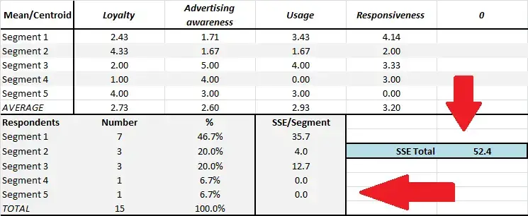
As the free Excel cluster analysis template automatically provides the output for two, three, four and five market segments – you need to choose the most appropriate number of segments for your marketing situation – and SSE will help you do that to some extent. Please check this diagram for where to locate the SSE scores on the Excel template – plus there a separate worksheet in the template that has two SSE charts for quick reference.

What is sum of squared error (SSE)?

Cluster analysis is a statistical technique designed to find the “best fit” of consumers (or respondents) to a particular market segment (cluster). It does this by performing repeated calculations (iterations) designed to bring the groups (segments) in tighter/closer. If the consumers matched the segment scores exactly, the the sum of squared error (SSE) would be zero = no error = a perfect match.

But with real world data, this is very unlikely to happen. So we need to look for a segmentation approach that has a lower SSE. The lower the SSE, then the more similar are the consumers in that market segment. A high SSE suggests that the consumers in the same market segment have a reasonable degree of differences between them and may not be a true (or usable) market segment.

Please note that you don’t need to select the segmentation approach with the lowest SSE, but it should be one of the lower ones.

Using SSE: An example (for SSE by Number of Segments)

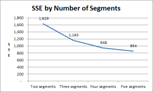To make sense of what to look for, let’s consider the following sum of squared error outputs:

With two segments = 1,629
With three segments = 1,163
With four segments = 948
With five market segments = 854

To further clarify, let’s have a look at these sum of squared error (SSE) outputs on a graph, as shown here. (This SSE chart is automatically produced by the template – you will find it on a separate worksheet – please see the tabs at the bottom of the spreadsheet.)

As you can see, as more market segments are created the SSE improves. This is generally to be expected. For example, if we had 100 consumers allocated to 100 different market segments, then the SSE would be zero – but, of course, it becomes impractical for a firm to pursue 100 market segments and, as well, each market segment would be too small to be viable.

Therefore, we need to accept a degree of error – (where “error” simply means that the consumers in each market segment are not completely identical, they will vary to some extent in terms of some of their behaviors and psychographic factors).

In this example, we would rule out the two market segment structure, as its SSE is too high relative to the other potential approaches – it is almost double the error of the five segment approach for instance.

The three segment approach offers a big improvement in minimizing SSE, but then the level of improvement starts to decrease (as to be expected) with each increment. I would suggest, that in this example, either the four or the five market segment structure would be suitable.

We also look at SSE per segment

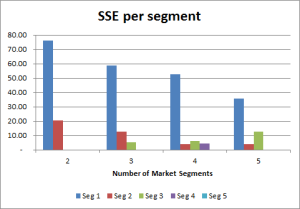While the previous SSE chart is quite helpful for looking at the overall “accuracy” of each of the segment structures to classify consumers, it is also worthwhile to consider the individual sum of squared errors for each segment. (Note: The sum of the individual segment SSE’s is equal to the total SSE.)

This information – SSE by segment – is available in both the “Output Clusters” and in the SSE charts worksheet, as shown here.

The lower the SSE, then the more similar (homogeneous) the consumers are in that market segment. If we look at the graph, we can see that segment one has a large SSE result across all segmentation structures. This indicates that there is some dissimilarity between the consumer in this market segment – and perhaps could be better defined?

However, the low SSE scores for the other segments indicate strong similarities between the consumers in each segment for the marketing variables being considered. For a segment with a SSE of zero – then that will be a segment of one consumer, or of identical consumer responses according to the data we are using.

Our final market segmentation decision

We would then make our final decision by also considering the marketing logic of these segments – look at the segmentation map and the average of each marketing variable – which one makes more sense based on what we know about the market and which one would be easier to construct a market strategy that would be successful?

Источник

What Is the Residual Sum of Squares (RSS)?

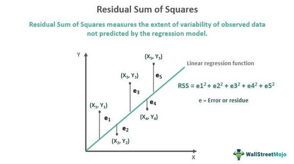
The residual sum of squares (RSS) is a statistical technique used to measure the amount of variance in a data set that is not explained by a regression model itself. Instead, it estimates the variance in the residuals, or error term.

Linear regression is a measurement that helps determine the strength of the relationship between a dependent variable and one or more other factors, known as independent or explanatory variables.

Key Takeaways

The residual sum of squares (RSS) measures the level of variance in the error term, or residuals, of a regression model.
The smaller the residual sum of squares, the better your model fits your data; the greater the residual sum of squares, the poorer your model fits your data.
A value of zero means your model is a perfect fit.
Statistical models are used by investors and portfolio managers to track an investment’s price and use that data to predict future movements.
The RSS is used by financial analysts in order to estimate the validity of their econometric models.

Understanding the Residual Sum of Squares

In general terms, the sum of squares is a statistical technique used in regression analysis to determine the dispersion of data points. In a regression analysis, the goal is to determine how well a data series can be fitted to a function that might help to explain how the data series was generated. The sum of squares is used as a mathematical way to find the function that best fits (varies least) from the data.

The RSS measures the amount of error remaining between the regression function and the data set after the model has been run. A smaller RSS figure represents a regression function that is well-fit to the data.

The RSS, also known as the sum of squared residuals, essentially determines how well a regression model explains or represents the data in the model.

How to Calculate the Residual Sum of Squares

RSS = ∑ⁿ_i=1(yⁱ — f(x_i))²

Where:

y_i = the i^th value of the variable to be predicted

f(x_i) = predicted value of y_i

n = upper limit of summation

Residual Sum of Squares (RSS) vs. Residual Standard Error (RSE)

The residual standard error (RSE) is another statistical term used to describe the difference in standard deviations of observed values versus predicted values as shown by points in a regression analysis. It is a goodness-of-fit measure that can be used to analyze how well a set of data points fit with the actual model.

RSE is computed by dividing the RSS by the number of observations in the sample less 2, and then taking the square root: RSE = [RSS/(n-2)]^1/2

Special Considerations

Financial markets have increasingly become more quantitatively driven; as such, in search of an edge, many investors are using advanced statistical techniques to aid in their decisions. Big data, machine learning, and artificial intelligence applications further necessitate the use of statistical properties to guide contemporary investment strategies. The residual sum of squares—or RSS statistics—is one of many statistical properties enjoying a renaissance.

Statistical models are used by investors and portfolio managers to track an investment’s price and use that data to predict future movements. The study—called regression analysis—might involve analyzing the relationship in price movements between a commodity and the stocks of companies engaged in producing the commodity.

Finding the residual sum of squares (RSS) by hand can be difficult and time-consuming. Because it involves a lot of subtracting, squaring, and summing, the calculations can be prone to errors. For this reason, you may decide to use software, such as Excel, to do the calculations.

Any model might have variances between the predicted values and actual results. Although the variances might be explained by the regression analysis, the RSS represents the variances or errors that are not explained.

Since a sufficiently complex regression function can be made to closely fit virtually any data set, further study is necessary to determine whether the regression function is, in fact, useful in explaining the variance of the dataset.

Typically, however, a smaller or lower value for the RSS is ideal in any model since it means there’s less variation in the data set. In other words, the lower the sum of squared residuals, the better the regression model is at explaining the data.

Example of the Residual Sum of Squares

For a simple (but lengthy) demonstration of the RSS calculation, consider the well-known correlation between a country’s consumer spending and its GDP. The following chart reflects the published values of consumer spending and Gross Domestic Product for the 27 states of the European Union, as of 2020.

Consumer Spending vs. GDP for EU Member States
Country	Consumer Spending (Millions)	GDP (Millions)
Austria	309,018.88	433,258.47
Belgium	388,436.00	521,861.29
Bulgaria	54,647.31	69,889.35
Croatia	47,392.86	57,203.78
Cyprus	20,592.74	24,612.65
Czech Republic	164,933.47	245,349.49
Denmark	251,478.47	356,084.87
Estonia	21,776.00	30,650.29
Finland	203,731.24	269,751.31
France	2,057,126.03	2,630,317.73
Germany	2,812,718.45	3,846,413.93
Greece	174,893.21	188,835.20
Hungary	110,323.35	155,808.44
Ireland	160,561.07	425,888.95
Italy	1,486,910.44	1,888,709.44
Latvia	25,776.74	33,707.32
Lithuania	43,679.20	56,546.96
Luxembourg	35,953.29	73,353.13
Malta	9,808.76	14,647.38
Netherlands	620,050.30	913,865.40
Poland	453,186.14	596,624.36
Portugal	190,509.98	228,539.25
Romania	198,867.77	248,715.55
Slovak Republic	83,845.27	105,172.56
Slovenia	37,929.24	53,589.61
Spain	997,452.45	1,281,484.64
Sweden	382,240.92	541,220.06

World Bank, 2020.

Consumer spending and GDP have a strong positive correlation, and it is possible to predict a country’s GDP based on consumer spending (CS). Using the formula for a best fit line, this relationship can be approximated as:

GDP = 1.3232 x CS + 10447

The units for both GDP and Consumer Spending are in millions of U.S. dollars.

This formula is highly accurate for most purposes, but it is not perfect, due to the individual variations in each country’s economy. The following chart compares the projected GDP of each country, based on the formula above, and the actual GDP as recorded by the World Bank.

Projected and Actual GDP Figures for EU Member States, and Residual Squares
Country	Consumer Spending Most Recent Value (Millions)	GDP Most Recent Value (Millions)	Projected GDP (Based on Trendline)	Residual Square (Projected — Real)^2
Austria	309,018.88	433,258.47	419,340.782016	193,702,038.819978
Belgium	388,436.00	521,861.29	524,425.52	6,575,250.87631504
Bulgaria	54,647.31	69,889.35	82,756.320592	165,558,932.215393
Croatia	47,392.86	57,203.78	73,157.232352	254,512,641.947534
Cyprus	20,592.74	24,612.65	37,695.313568	171,156,086.033474
Czech Republic	164,933.47	245,349.49	228,686.967504	277,639,655.929706
Denmark	251,478.47	356,084.87	343,203.311504	165,934,549.28587
Estonia	21,776.00	30,650.29	39,261.00	74,144,381.8126542
Finland	203,731.24	269,751.31	280,024.176768	105,531,791.633079
France	2,057,126.03	2,630,317.73	2,732,436.162896	10,428,174,337.1349
Germany	2,812,718.45	3,846,413.93	3,732,236.05304	13,036,587,587.0929
Greece	174,893.21	188,835.20	241,865.695472	2,812,233,450.00581
Hungary	110,323.35	155,808.44	156,426.85672	382,439.239575558
Ireland	160,561.07	425,888.95	222,901.407824	41,203,942,278.6534
Italy	1,486,910.44	1,888,709.44	1,977,926.894208	7,959,754,135.35658
Latvia	25,776.74	33,707.32	44,554.782368	117,667,439.825176
Lithuania	43,679.20	56,546.96	68,243.32	136,804,777.364243
Luxembourg	35,953.29	73,353.13	58,020.393328	235,092,813.852894
Malta	9,808.76	14,647.38	23,425.951232	77,063,312.875298
Netherlands	620,050.30	913,865.40	830,897.56	6,883,662,978.71
Poland	453,186.14	596,624.36	610,102.900448	181,671,052.608372
Portugal	190,509.98	228,539.25	262,529.805536	1,155,357,865.6459
Romania	198,867.77	248,715.55	273,588.833264	618,680,220.331183
Slovak Republic	83,845.27	105,172.56	121,391.061264	263,039,783.25037
Slovenia	37,929.24	53,589.61	60,634.970368	49,637,102.7149851
Spain	997,452.45	1,281,484.64	1,330,276.08184	2,380,604,796.8261
Sweden	382,240.92	541,220.06	516,228.185344	624,593,798.821215

World Bank, 2020.

The column on the right indicates the residual squares–the squared difference between each projected value and its actual value. The numbers appear large, but their sum is actually lower than the RSS for any other possible trendline. If a different line had a lower RSS for these data points, that line would be the best fit line.

Is the Residual Sum of Squares the Same as R-Squared?

The residual sum of squares (RSS) is the absolute amount of explained variation, whereas R-squared is the absolute amount of variation as a proportion of total variation.

Is RSS the Same as the Sum of Squared Estimate of Errors (SSE)?

The residual sum of squares (RSS) is also known as the sum of squared estimate of errors (SSE).

What Is the Difference Between the Residual Sum of Squares and Total Sum of Squares?

The total sum of squares (TSS) measures how much variation there is in the observed data, while the residual sum of squares measures the variation in the error between the observed data and modeled values. In statistics, the values for the residual sum of squares and the total sum of squares (TSS) are oftentimes compared to each other.

Can a Residual Sum of Squares Be Zero?

The residual sum of squares can be zero. The smaller the residual sum of squares, the better your model fits your data; the greater the residual sum of squares, the poorer your model fits your data. A value of zero means your model is a perfect fit.

Источник

You may be wondering what all of those sums of squares are all about. Maybe that’s what got you here in the first place. Well, they are the determinants of a good linear regression. This tutorial is based on the ANOVA framework you may have heard before.

Before reading it, though, make sure you are not mistaking regression for correlation. If you’ve got this checked, we can get straight into the action.

A quick side-note: Want to learn more about linear regression? Check out our explainer videos The Linear Regression Model. Geometrical Representation and The Simple Linear Regression Model.

SST, SSR, SSE: Definition and Formulas

There are three terms we must define. The sum of squares total, the sum of squares regression, and the sum of squares error.

What is the SST?

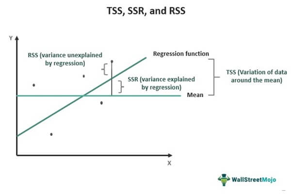
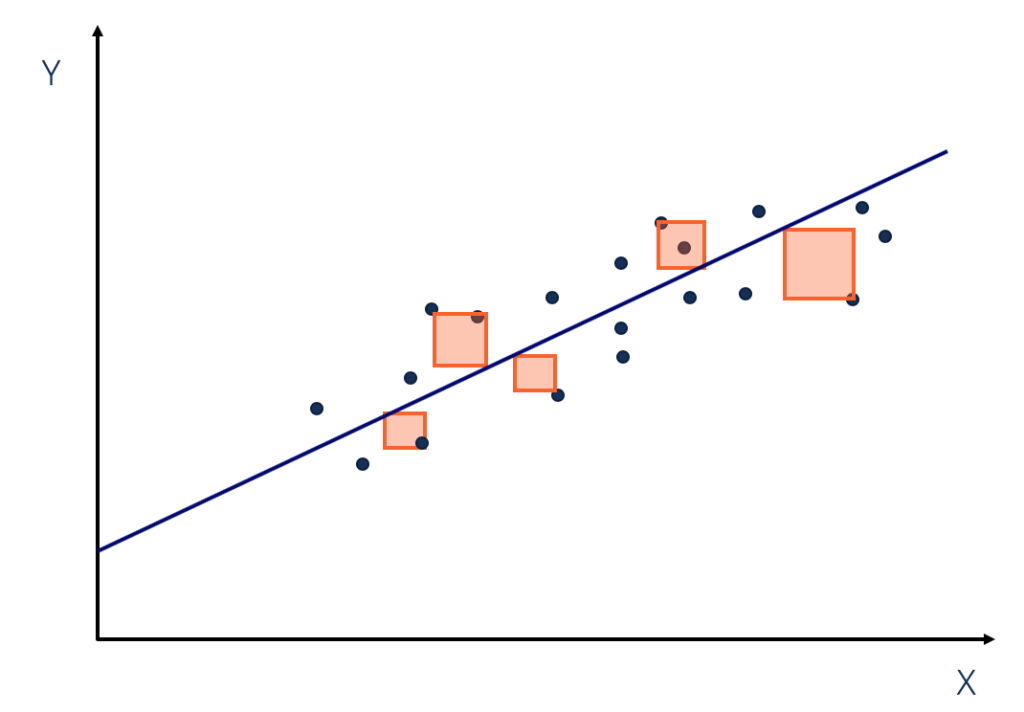
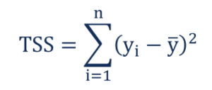
The sum of squares total, denoted SST, is the squared differences between the observed dependent variable and its mean. You can think of this as the dispersion of the observed variables around the mean – much like the variance in descriptive statistics.

It is a measure of the total variability of the dataset.

Side note: There is another notation for the SST. It is TSS or total sum of squares.

What is the SSR?

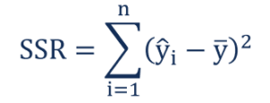
The second term is the sum of squares due to regression, or SSR. It is the sum of the differences between the predicted value and the mean of the dependent variable. Think of it as a measure that describes how well our line fits the data.

If this value of SSR is equal to the sum of squares total, it means our regression model captures all the observed variability and is perfect. Once again, we have to mention that another common notation is ESS or explained sum of squares.

What is the SSE?

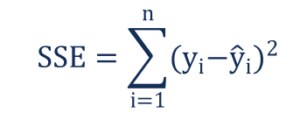
The last term is the sum of squares error, or SSE. The error is the difference between the observed value and the predicted value.

We usually want to minimize the error. The smaller the error, the better the estimation power of the regression. Finally, I should add that it is also known as RSS or residual sum of squares. Residual as in: remaining or unexplained.

The Confusion between the Different Abbreviations

It becomes really confusing because some people denote it as SSR. This makes it unclear whether we are talking about the sum of squares due to regression or sum of squared residuals.

In any case, neither of these are universally adopted, so the confusion remains and we’ll have to live with it.

Simply remember that the two notations are SST, SSR, SSE, or TSS, ESS, RSS.

There’s a conflict regarding the abbreviations, but not about the concept and its application. So, let’s focus on that.

How Are They Related?

Mathematically, SST = SSR + SSE.

The rationale is the following: the total variability of the data set is equal to the variability explained by the regression line plus the unexplained variability, known as error.

Given a constant total variability, a lower error will cause a better regression. Conversely, a higher error will cause a less powerful regression. And that’s what you must remember, no matter the notation.

Next Step: The R-squared

Well, if you are not sure why we need all those sums of squares, we have just the right tool for you. The R-squared. Care to learn more? Just dive into the linked tutorial where you will understand how it measures the explanatory power of a linear regression!

***

Interested in learning more? You can take your skills from good to great with our statistics course.

Try statistics course for free

Next Tutorial: Measuring Variability with the R-squared

Источник

Residual Sum of Squares (RSS) is a statistical method that helps identify the level of discrepancy in a dataset not predicted by a regression model. Thus, it measures the variance in the value of the observed data when compared to its predicted value as per the regression model. Hence, RSS indicates whether the regression model fits the actual dataset well or not.

You are free to use this image on your website, templates, etc., Please provide us with an attribution linkArticle Link to be Hyperlinked
For eg:
Source: Residual sum of squares (wallstreetmojo.com)

Also referred to as the Sum of Squared Errors (SSE), RSS is obtained by adding the square of residuals. Residuals are projected deviations from actual data values and represent errors in the regression Regression Analysis is a statistical approach for evaluating the relationship between 1 dependent variable & 1 or more independent variables. It is widely used in investing & financing sectors to improve the products & services further. read moremodel’s estimation. A lower RSS indicates that the regression model fits the data well and has minimal data variation. In financeFinance is a broad term that essentially refers to money management or channeling money for various purposes.read more, investors use RSS to track the changes in the prices of a stock to predict its future price movements.

What is Residual Sum of Squares?
- Residual Sum of Squares Explained
- Residual Sum of Squares in Finance
- Formula
- Calculation Example
- Frequently Asked Questions (FAQs)
- Recommended Articles

Residual Sum of Squares (RSS) is a statistical method used to measure the deviation in a dataset unexplained by the regression model.
Residual or error is the difference between the observation’s actual and predicted value.
If the RSS value is low, it means the data fits the estimation model well, indicating the least variance. If it is zero, the model fits perfectly with the data, having no variance at all.
It helps stock market players to assess the future stock price movements by monitoring the fluctuation in the stock prices.

Residual Sum of Squares Explained

RSS is one of the types of the Sum of Squares (SS) – the rest two being the Total Sum of Squares (TSS) and Sum of Squares due to Regression (SSR) or Explained Sum of Squares (ESS). Sum of squares is a statistical measure through which the data dispersion In statistics, dispersion (or spread) is a means of describing the extent of distribution of data around a central value or point. It aids in understanding data distribution.read moreis assessed to determine how well the data would fit the model in regression analysis.

While the TSS measures the variation in values of an observed variable with respect to its sample mean, the SSR or ESS calculates the deviation between the estimated value and the mean value of the observed variable. If the TSS equals SSR, it means the regression model is a perfect fit for the data as it reflects all the variability in the actual data.

You are free to use this image on your website, templates, etc., Please provide us with an attribution linkArticle Link to be Hyperlinked
For eg:
Source: Residual sum of squares (wallstreetmojo.com)

On the other hand, RSS measures the extent of variability of observed data not shown by a regression model. To calculate RSS, first find the model’s level of error or residue by subtracting the actual observed values from the estimated values. Then, square and add all error values to arrive at RSS.

The lower the error in the model, the better the regression prediction. In other words, a lower RSS signifies that the regression model explains the data better, indicating the least variance. It means the model fits the data well. Likewise, if the value comes to zero, it’s considered the best fit with no variance.

Note that the RSS is not similar to R-SquaredR-squared ( R2 or Coefficient of Determination) is a statistical measure that indicates the extent of variation in a dependent variable due to an independent variable.read more. While the former defines the exact amount of variation, R-squared is the amount of variation defined with respect to the proportion of total variation.

Residual Sum of Squares in Finance

The discrepancy detected in the data set through RSS indicates whether the data is a fit or misfit to the regression model. Thus, it helps stock marketStock Market works on the basic principle of matching supply and demand through an auction process where investors are willing to pay a certain amount for an asset, and they are willing to sell off something they have at a specific price.read more players to understand the fluctuation occurring in the asset prices, letting them assess their future price movements.

Regression functions are formed to predict the movement of stock prices. But the benefit of these regression models depends on whether they well explain the variance in stock prices. However, if there are errors or residuals in the model unexplained by regression, then the model may not be useful in predicting future stock movements.

As a result, the investors and money managers get an opportunity to make the best and most well-informed decisions using RSS. In addition, RSS also lets policymakers analyze various variables affecting the economic stability of a nation and frame the economic models accordingly.

Formula

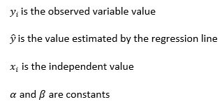
Here is the formula to calculate the residual sum of squares:

Where,

Calculation Example

Let’s consider the following residual sum of squares example based on the set of data below:

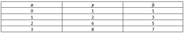
The absolute variance can be easily found out by implementing the above RSS formula:

= {1 – [1+(2*0)]}² + {2 – [1+(2*1)]}²+ {6 – [1+(2*2)]}² + {8 – [1+(2*3)]}²

= 0+1+1+1 = 3

Frequently Asked Questions (FAQs)

What is Residual Sum of Squares (RSS)?

RSS is a statistical method used to detect the level of discrepancy in a dataset not revealed by regression. If the residual sum of squares results in a lower figure, it signifies that the regression model explains the data better than when the result is higher. In fact, if its value is zero, it’s regarded as the best fit with no error at all.

What is the difference between ESS and RSS?

ESS stands for Explained Sum of Squares, which marks the variation in the data explained by the regression model. On the other hand, Residual Sum of Squares (RSS) defines the variations marked by the discrepancies in the dataset not explained by the estimation model.

How do TSS and RSS differ?

The Total Sum of Squares (TSS) defines the variations in the observed values or datasets from the mean. In contrast, the Residual Sum of Squares (RSS) assesses the errors or discrepancies in the observed data and the modeled data.

What is Sum of Squares?

Sum of squares (SS) is a statistical tool that is used to identify the dispersion of data as well as how well the data can fit the model in regression analysis. The sum of squares got its name because it is calculated by finding the sum of the squared differences.

This image is only for illustrative purposes.

The sum of squares is one of the most important outputs in regression analysis. The general rule is that a smaller sum of squares indicates a better model, as there is less variation in the data.

In finance, understanding the sum of squares is important because linear regression models are widely used in both theoretical and practical finance.

Types of Sum of Squares

In regression analysis, the three main types of sum of squares are the total sum of squares, regression sum of squares, and residual sum of squares.

1. Total sum of squares

The total sum of squares is a variation of the values of a dependent variable from the sample mean of the dependent variable. Essentially, the total sum of squares quantifies the total variation in a sample. It can be determined using the following formula:

Where:

y_i– the value in a sample
ȳ – the mean value of a sample

2. Regression sum of squares (also known as the sum of squares due to regression or explained sum of squares)

The regression sum of squares describes how well a regression model represents the modeled data. A higher regression sum of squares indicates that the model does not fit the data well.

The formula for calculating the regression sum of squares is:

Where:

ŷ_i– the value estimated by the regression line
ȳ – the mean value of a sample

3. Residual sum of squares (also known as the sum of squared errors of prediction)

The residual sum of squares essentially measures the variation of modeling errors. In other words, it depicts how the variation in the dependent variable in a regression model cannot be explained by the model. Generally, a lower residual sum of squares indicates that the regression model can better explain the data, while a higher residual sum of squares indicates that the model poorly explains the data.

The residual sum of squares can be found using the formula below:

Where:

y_i– the observed value
ŷ_i– the value estimated by the regression line

The relationship between the three types of sum of squares can be summarized by the following equation:

Additional Resources

Thank you for reading CFI’s guide to Sum of Squares. To keep learning and advancing your career, the following CFI resources will be helpful:

Free Data Science Course
Guide to Financial Modeling
Harmonic Mean
Hypothesis Testing
3 Statement Model
See all data science resources

Источник

One explanatory variable[edit]

Matrix expression for the OLS residual sum of squares[edit]

Relation with Pearson’s product-moment correlation[edit]

See also[edit]

References[edit]

References

About This Article

Did this article help you?

What is sum of squared error (SSE)?

Using SSE: An example (for SSE by Number of Segments)

We also look at SSE per segment

Our final market segmentation decision

What Is the Residual Sum of Squares (RSS)?

Key Takeaways

Understanding the Residual Sum of Squares

How to Calculate the Residual Sum of Squares

Residual Sum of Squares (RSS) vs. Residual Standard Error (RSE)

Special Considerations

Example of the Residual Sum of Squares

Is the Residual Sum of Squares the Same as R-Squared?

Is RSS the Same as the Sum of Squared Estimate of Errors (SSE)?

What Is the Difference Between the Residual Sum of Squares and Total Sum of Squares?

Can a Residual Sum of Squares Be Zero?

SST, SSR, SSE: Definition and Formulas

What is the SST?

What is the SSR?

What is the SSE?

The Confusion between the Different Abbreviations

How Are They Related?

Next Step: The R-squared

Table of contents

Residual Sum of Squares Explained

Residual Sum of Squares in Finance

Formula

Calculation Example

Frequently Asked Questions (FAQs)

Recommended Articles

What is Sum of Squares?

Types of Sum of Squares

1. Total sum of squares

2. Regression sum of squares (also known as the sum of squares due to regression or explained sum of squares)

3. Residual sum of squares (also known as the sum of squared errors of prediction)

Additional Resources