What is a Systematic Error?
Systematic error as the name implies is a consistent or reoccurring error that is caused by incorrect use or generally bad experimental equipment. With systematic error, you can expect the result of each experiment to differ from the value in the original data.
This is also known as systematic bias because the errors will hide the correct result, thus leading the researcher to wrong conclusions
In the following paragraphs, we are going to explore the types of systematic errors, the causes of these errors, how to identify the systematic error, and how you can avoid it in your research.
Use for free: Equipment Inspection Form Template
Types of Systematic Errors
There are two types of systematic error which are offset error and scale factor error. These two types of systematic errors have their distinct attributes as will be seen below.
1. Offset Error
Before starting your experiment, your scale should be set to zero points. The offset error occurs when the measurement scale is not set to zero points before weighing your items.
For example, if you’re familiar with a kitchen scale, you’ll notice it has a button labeled tare. This tare button sets the scale to point zero before you weigh your item on the scale. If this tare button is not used correctly, then all measurements will have an offset error since zero will not be the starting point of the values on the measurement scale.
Another name for offset error is the zero-setting error.
Read: Research Bias: Definition, Types + Example, Types + Example Research Bias: Definition, Types + Exam
2. Scale Factor Error
This is also known as multiple errors.
The scale factor error results from changes in the value or size of your scale that differs from its actual size.
Let us consider a scenario whereby your scale repeatedly adds an extra 5% to your measurements. So when you’re measuring a value of 10kg, your scale shows a result of 10.5kg.
The implication is that, because the scale is not reading at its original value which should be zero, for every stretch, your measurement will also be read incorrectly. If the scale increases by 1%, your reading will also increase by 1%. What scale factor error does is that through percentage or proportion, it adds or deduct from the original value.
One thing to note is that systematic error is always consistent. If it brings a value of say 70g at the first reading, and you decide to conduct the measurement again, it will still give you the same reading as before.
Also, both offset error and scale factor error can be plotted in a graph to identify how they differ from each other.
Look at the graphs below, the black line represents the result of your research data being equal to the original value and the blue line in the graph represents an offset error.
We have earlier established that offset error shifts your data value by increasing or decreasing it at a consistent value. If you observe the blue line, you’d realize it added one extra unit to the data.
The second graph with a pink line represents the scale factor error. Scale factor error shifts your data value proportionally, to a similar direction.
Here, all values are shifted proportionally the same way, but by different degrees.
Read Also – Type I vs Type II Errors: Causes, Examples & Prevention
Causes of Systematic Errors in Research
The two primary causes of systematic error are faulty instruments or equipment and improper use of instruments.
There are other ways systematic error can happen in your experiments, and these could be the research data, confounding, the procedure you used to gather your data, and even your analysis method.
Briefly, we will discuss the two primary causes of systematic error and also look at one other cause which is known as the analysis method.
- Researcher’s Error
When a researcher is ignorant, has a physical challenge that can cause an effect on a study, or is just careless, it can alter the outcome of the research. Preventing any of the above-listed traits as a researcher can immensely reduce the likelihood of making errors in your research.
- Instrument Error
Systematic errors can happen if your equipment is faulty. The imperfection of your experiment equipment can alter your study and ultimately, its findings.
- Analysis method Error
As a researcher, if you do not plan how you’ll control your experiment in advance, your research is at risk of being inaccurate. So to reduce the risk of error in your research, try as much as possible to limit your independent variables to only one. The lesser your variables in an analysis, the more chance you have to error-free research.
Generally, a systematic error can occur if you as a researcher repeatedly take the wrong measurements, if your measuring tape has stretched from its initial point perhaps because of many years of use or if your scale reads zero when a container or your value is placed on it.
Read: Survey Scale: Definitions, Types + [Question Examples]
Effects of Systematic Errors on Research
The effect of a systematic error in research is that it will move the value of your measurements away from their original value by the same percentage or the same proportion while in the same direction.
The consequence is that shifting the measurement does not affect your reliability. This is because irrespective of how many times you repeat the measurement, you will get the same value. However, the effect is on the accuracy of your result. If you’re not careful enough to notice the inaccuracy, you might draw the wrong conclusion or even apply the wrong solutions.
Read: Margin of error – Definition, Formula + Application
How Do you Identify Systematic Errors?
You cannot easily detect a Systematic error in your study. In fact, you may not recognize systematic errors even with the visualization method.
You need to make use of statistical analysis to identify the type of error present in your research and assess the error. When your study findings have the desired outcome, then there is no systematic error.
You can also identify the systematic error by comparing the result from your analysis to the standard. If the two results differ, then there may be systematic bias.
You can use standard data or known theoretical results as a reference to detect and determine the systematic errors in your research.
Usually, when you analyze the result of your data, you may expect your result to show that your original data are randomly distributed. However, the consistent increase or decrease of the result of your research data will tell you if a systematic bias exists in your data.
Once you identify any systematic error in your research, apply the treatment condition to correct it and calibrate immediately.
Read: Survey Errors To Avoid: Types, Sources, Examples, Mitigation
Examples of Systematic Errors in Research
We are going to look at the following examples to better understand the concept of systematic error.
Example one:
Let’s assume some researchers are carrying out a study on weight loss. At the end of the research, the researchers realized the scale added 15 pounds to each of the sample data, they then concluded that their finding is inaccurate because the scale used gave a wrong reading. Now, this is an example of a systematic error, because the error, although consistent, is inaccurate. If the researchers did not realize the disparity, they would have made a wrong conclusion.
This example shows how systematic errors can occur in research because of faulty instruments. Therefore, frequent calibration is advised before conducting a test.
Example two:
When measuring the temperature of a room, if your thermometer and the room you’re measuring are in poor contact, you will get an inaccurate reading. If you repeat the test and your thermometer still has low thermal contact with the room, you will get constant results even though inaccurate. Here, the thermometer is not faulty, the cause of the error is the researcher’s wrongful handling.
These two examples show that systematic error can arise from faulty instruments and wrong usage of the instrument. If you do not get a result close to the true value of your data, consider identifying the cause of the error and how to reduce it.
How to Minimize or Avoid Systematic Errors in Research
Once you can identify the cause of a systematic error, you should be able to reduce its effect on your data to a great extent.
The issue, however, is that systematic errors are not easily detectable. This is because your equipment cannot talk, so you won’t get a warning signal, and regardless of how many times you conduct the test, you will arrive at the same result which can be confusing.
So how should you go about this? You should first make sure that you understand your equipment and its features.
Use For Free: Equipment Maintenance Log Template
This will allow you to know the limitations of your equipment. If you are using a voltmeter on a circuit, it may give you varied voltage readings depending on the condition of whether it’s a high current or low current voltage.
If you’re conducting a test on a computer program, confirm in advance if the program works accurately. You can do this by testing data whose value had been previously determined. That way you are certain of what the outcome should be so if you get a different result, you know something is not right.
Once you understand where the issue is, you can reduce systematic error by properly setting up your equipment. Test your equipment before conducting the actual reading and always compare the value from your reading against the standards or theoretical result.
FAQs about Systematic Errors in Research
- What is the difference between systematic and random error?
As the name suggests, random error is always random. You cannot predict it and you cannot get the same reading if you repeat the measurement or analysis. You will always get a unique value (random value).
For example, let us assume you weighed a bag of grains on a scale, the first time, you might get a value of 140 lbs, if you tried again, you may arrive at 125 lbs. Regardless of the number of times you repeat the measurement, you will get a different or random error.
Systematic errors are always consistent with the error. Even if you repeat the process, you will still arrive at the same error.
For example, if your measurement is 80g, and your measuring tape is stretched by 99mm, either as an addition or deduction, if you repeat the measurement, the reading you will get will be the same as before. The error will be consistent.
- How can we eliminate systematic error?
Systematic errors can be eliminated by using one of these methods in your research.
Triangulation: This is the method of using over one technique to document your research observations. That way you don’t rely on one piece of equipment or technique. When you’re done with your testing, you can easily compare the findings from your multiple techniques and see whether they match or they don’t.
Frequent calibration: This means that you compare the findings from your test to the standard value or theoretical result. Doing this regularly with a standard result to cross-check can reduce the chance of systematic error in your research.
When you’re conducting research, make sure you do routine checks. If you’re wondering how often you should perform calibration, note that this generally depends on your equipment.
Randomization: Using randomization in your study can reduce the risk of systematic error because when you’re testing your data, you can randomly group your data sample into a relevant treatment group. That will even the sample size across their groups.
- Which is worse, systematic or random error?
Both systematic error and random error are not to be desired. However, systematic error is a more difficult problem to have in research. This is because it takes your findings away from the correct value and this can lead to false conclusions.
When you have a random error in your research, you know that the result of your measurements can either increase or decrease just a little from the real value. If you average these results, you are likely to get close to the actual value. But if your measurements have a systematic error, your findings will be rather far from the true value.
Two Types of Experimental Error
No matter how careful you are, there is always error in a measurement. Error is not a «mistake»—it’s part of the measuring process. In science, measurement error is called experimental error or observational error.
There are two broad classes of observational errors: random error and systematic error. Random error varies unpredictably from one measurement to another, while systematic error has the same value or proportion for every measurement. Random errors are unavoidable, but cluster around the true value. Systematic error can often be avoided by calibrating equipment, but if left uncorrected, can lead to measurements far from the true value.
Key Takeaways
- Random error causes one measurement to differ slightly from the next. It comes from unpredictable changes during an experiment.
- Systematic error always affects measurements the same amount or by the same proportion, provided that a reading is taken the same way each time. It is predictable.
- Random errors cannot be eliminated from an experiment, but most systematic errors can be reduced.
Random Error Example and Causes
If you take multiple measurements, the values cluster around the true value. Thus, random error primarily affects precision. Typically, random error affects the last significant digit of a measurement.
The main reasons for random error are limitations of instruments, environmental factors, and slight variations in procedure. For example:
- When weighing yourself on a scale, you position yourself slightly differently each time.
- When taking a volume reading in a flask, you may read the value from a different angle each time.
- Measuring the mass of a sample on an analytical balance may produce different values as air currents affect the balance or as water enters and leaves the specimen.
- Measuring your height is affected by minor posture changes.
- Measuring wind velocity depends on the height and time at which a measurement is taken. Multiple readings must be taken and averaged because gusts and changes in direction affect the value.
- Readings must be estimated when they fall between marks on a scale or when the thickness of a measurement marking is taken into account.
Because random error always occurs and cannot be predicted, it’s important to take multiple data points and average them to get a sense of the amount of variation and estimate the true value.
Systematic Error Example and Causes
Systematic error is predictable and either constant or else proportional to the measurement. Systematic errors primarily influence a measurement’s accuracy.
Typical causes of systematic error include observational error, imperfect instrument calibration, and environmental interference. For example:
- Forgetting to tare or zero a balance produces mass measurements that are always «off» by the same amount. An error caused by not setting an instrument to zero prior to its use is called an offset error.
- Not reading the meniscus at eye level for a volume measurement will always result in an inaccurate reading. The value will be consistently low or high, depending on whether the reading is taken from above or below the mark.
- Measuring length with a metal ruler will give a different result at a cold temperature than at a hot temperature, due to thermal expansion of the material.
- An improperly calibrated thermometer may give accurate readings within a certain temperature range, but become inaccurate at higher or lower temperatures.
- Measured distance is different using a new cloth measuring tape versus an older, stretched one. Proportional errors of this type are called scale factor errors.
- Drift occurs when successive readings become consistently lower or higher over time. Electronic equipment tends to be susceptible to drift. Many other instruments are affected by (usually positive) drift, as the device warms up.
Once its cause is identified, systematic error may be reduced to an extent. Systematic error can be minimized by routinely calibrating equipment, using controls in experiments, warming up instruments prior to taking readings, and comparing values against standards.
While random errors can be minimized by increasing sample size and averaging data, it’s harder to compensate for systematic error. The best way to avoid systematic error is to be familiar with the limitations of instruments and experienced with their correct use.
Key Takeaways: Random Error vs. Systematic Error
- The two main types of measurement error are random error and systematic error.
- Random error causes one measurement to differ slightly from the next. It comes from unpredictable changes during an experiment.
- Systematic error always affects measurements the same amount or by the same proportion, provided that a reading is taken the same way each time. It is predictable.
- Random errors cannot be eliminated from an experiment, but most systematic errors may be reduced.
Sources
- Bland, J. Martin, and Douglas G. Altman (1996). «Statistics Notes: Measurement Error.» BMJ 313.7059: 744.
- Cochran, W. G. (1968). «Errors of Measurement in Statistics». Technometrics. Taylor & Francis, Ltd. on behalf of American Statistical Association and American Society for Quality. 10: 637–666. doi:10.2307/1267450
- Dodge, Y. (2003). The Oxford Dictionary of Statistical Terms. OUP. ISBN 0-19-920613-9.
- Taylor, J. R. (1999). An Introduction to Error Analysis: The Study of Uncertainties in Physical Measurements. University Science Books. p. 94. ISBN 0-935702-75-X.
Experimental techniques
Yanqiu Huang, … Zhixiang Cao, in Industrial Ventilation Design Guidebook (Second Edition), 2021
4.3.3.2 Measurement errors
The measurement errors are divided into two categories: systematic errors and random errors (OIML, 1978).
Systematic error is an error which, in the course of a number of measurements carried out under the same conditions of a given value and quantity, either remains constant in absolute value and sign, or varies according to definite law with changing conditions.
Random error varies in an unpredictable manner in absolute value and in sign when a large number of measurements of the same value of a quantity are made under essentially identical conditions.
The origins of the above two errors are different in cause and nature. A simple example is when the mass of a weight is less than its nominal value, a systematic error occurs, which is constant in absolute value and sign. This is a pure systematic error. A ventilation-related example is when the instrument factor of a Pitot-static tube, which defines the relationship between the measured pressure difference and the velocity, is incorrect, a systematic error occurs. On the other hand, if a Pitot-static tube is positioned manually in a duct in such a way that the tube tip is randomly on either side of the intended measurement point, a random error occurs. This way, different phenomena create different types of error. The (total) error of measurement usually is a combination of the above two types.
The question may be asked, that is, what is the reason for dividing the errors into two categories? The answer is the totally different way of dealing with these different types. Systematic error can be eliminated to a sufficient degree, whereas random error cannot. The following section shows how to deal with these errors.
Read full chapter
URL:
https://www.sciencedirect.com/science/article/pii/B9780128166734000043
EXPERIMENTAL TECHNIQUES
KAI SIREN, … PETER V. NIELSEN, in Industrial Ventilation Design Guidebook, 2001
12.3.3.11 Systematic Errors
Systematic error, as stated above, can be eliminated—not totally, but usually to a sufficient degree. This elimination process is called “calibration.” Calibration is simply a procedure where the result of measurement recorded by an instrument is compared with the measurement result of a standard. A standard is a measuring device intended to define, to represent physically, to conserve, or to reproduce the unit of measurement in order to transmit it to other measuring instruments by comparison.1 There are several categories of standards, but, simplifying a little, a standard is an instrument with a very high accuracy and can for that reason be used as a reference for ordinary measuring instruments. The calibration itself is usually carried out by measuring the quantity over the whole range required and by defining either one correction factor for the whole range, for a constant systematic error, or a correction curve or equation for the whole range. Applying this correction to the measurement result eliminates, more or less, the systematic error and gives the corrected result of measurement.
A primary standard has the highest metrological quality in a given field. Hence, the primary standard is the most accurate way to measure or to reproduce the value of a quantity. Primary standards are usually complicated instruments, which are essentially laboratory instruments and unsuited for site measurement. They require skilled handling and can be expensive. For these reasons it is not practical to calibrate all ordinary meters against a primary standard. To utilize the solid metrological basis of the primary standard, a chain of secondary standards, reference standards, and working standards combine the primary standard and the ordinary instruments. The lower level standard in the chain is calibrated using the next higher level standard. This is called “traceability.” In all calibrations traceability along the chain should exist, up to the instrument with the highest reliability, the primary standard.
The question is often asked, How often should calibration be carried out? Is it sufficient to do it once, or should it be repeated? The answer to this question depends on the instrument type. A very simple instrument that is robust and stable may require calibrating only once during its lifetime. Some fundamental meters do not need calibration at all. A Pitot-static tube or a liquid U-tube manometer are examples of such simple instruments. On the other hand, complicated instruments with many components or sensitive components may need calibration at short intervals. Also fouling and wearing are reasons not only for maintenance but also calibration. Thus the proper calibration interval depends on the instrument itself and its use. The manufacturers recommendations as well as past experience are often the only guidelines.
Read full chapter
URL:
https://www.sciencedirect.com/science/article/pii/B9780122896767500151
Intelligent control and protection in the Russian electric power system
Nikolai Voropai, … Daniil Panasetsky, in Application of Smart Grid Technologies, 2018
3.3.1.2 Systematic errors in PMU measurements
The systematic errors caused by the errors of the instrument transformers that exceed the class of their accuracy are constantly present in the measurements and can be identified by considering some successive snapshots of measurements. The TE linearized at the point of a true measurement, taking into account random and systematic errors, can be written as:
(25)wky¯=∑l∈ωk∂w∂ylξyl+cyl=∑aklξyl+∑aklcyl
where ∑ aklξyl—mathematical expectation of random errors of the TE, equal to zero; ∑ aklcyl—mathematical expectation of systematic error of the TE, ωk—a set of measurements contained in the kth TE.
The author of Ref. [28] suggests an algorithm for the identification of a systematic component of the measurement error on the basis of the current discrepancy of the TE. The algorithm rests on the fact that systematic errors of measurements do not change through a long time interval. In this case, condition (17) will not be met during such an interval of time. Based on the snapshots that arrive at time instants 0, 1, 2, …, t − 1, t…, the sliding average method is used to calculate the mathematical expectation of the TE discrepancy:
(26)Δwkt=1−αΔwkt−1+αwkt
where 0 ≤ α ≤ 1.
Fig. 5 shows the curve of the TE discrepancy (a thin dotted line) calculated by (26) for 100 snapshots of measurements that do not have systematic errors.

Fig. 5. Detection of a systematic error in the PMU measurements and identification of mathematical expectation of the test equation.
It virtually does not exceed the threshold dk = 0.014 (a light horizontal line). Above the threshold, there is a curve of the TE discrepancy (a bold dotted line) that contains a measurement with a systematic error and a curve of nonzero mathematical expectation Δwk(t) ∈ [0.026; 0.03] (a black-blue thick line). However, the nonzero value of the calculated mathematical expectation of the TE discrepancy can only testify to the presence of a systematic error in the PMU measurements contained in this TE, but cannot be used to locate it.
Read full chapter
URL:
https://www.sciencedirect.com/science/article/pii/B9780128031285000039
Measurements
Sankara Papavinasam, in Corrosion Control in the Oil and Gas Industry, 2014
ii Systematic or determinate error
To define systematic error, one needs to understand ‘accuracy’. Accuracy is a measure of the closeness of the data to its true or accepted value. Figure 12.3 illustrates accuracy schematically.4 Determining the accuracy of a measurement is difficult because the true value may never be known, so for this reason an accepted value is commonly used. Systematic error moves the mean or average value of a measurement from the true or accepted value.

FIGURE 12.3. Difference between Accuracy and Precision in a Measurement.4
Reproduced with permission from Brooks/Cole, A Division of Cengage Learning.
Systematic error may be expressed as absolute error or relative error:
- •
-
The absolute error (EA) is a measure of the difference between the measured value (xi) and true or accepted value (xt) (Eqn. 12.5):
(Eqn. 12.5)EA=xi−xt
Absolute error bears a sign:
- •
-
A negative sign indicates that the measured value is smaller than true value and
- •
-
A positive sign indicates that the measured value is higher than true value
The relative error (ER) is the ratio of measured value to true value and it is expressed as (Eqn. 12.6):
(Eqn. 12.6)ER=(xi−xtxt).100
Table 12.2 illustrates the absolute and relative errors for six measurements in determining the concentration of 20 ppm of an ionic species in solution.
Table 12.2. Relative and Absolute Errors in Six Measurements of Aqueous Solution Containing 20 ppm of an Ionic Species
| Measured Value | Absolute Error | Relative Error (Percentage) | Remarks |
|---|---|---|---|
| 19.4 | −0.6 | −3.0 | Experimental value lower than actual value. |
| 19.5 | −0.5 | −2.5 | |
| 19.6 | −0.4 | −2.0 | |
| 19.8 | −0.2 | −1.0 | |
| 20.1 | +0.1 | +0.5 | Experimental value higher than actual value. |
| 20.3 | +0.3 | +1.5 |
Systematic error may occur due to instrument, methodology, and personal error.
Instrument error
Instrument error occurs due to variations that can affect the functionality of the instrument. Some common causes include temperature change, voltage fluctuation, variations in resistance, distortion of the container, error from original calibration, and contamination. Most instrument errors can be detected and corrected by frequently calibrating the instrument using a standard reference material. Standard reference materials may occur in different forms including minerals, gas mixtures, hydrocarbon mixtures, polymers, solutions of known concentration of chemicals, weight, and volume. The standard reference materials may be prepared in the laboratory or may be obtained from standard-making organizations (e.g., ASTM standard reference materials), government agencies (e.g., National Institute of Standards and Technology (NIST) provides about 900 reference materials) and commercial suppliers. If standard materials are not available, a blank test may be performed using a solution without the sample. The value from this test may be used to correct the results from the actual sample. However this methodology may not be applicable for correcting instrumental error in all situations.
Methodology error
Methodology error occurs due to the non-ideal physical or chemical behavior of the method. Some common causes include variation of chemical reaction and its rate, incompleteness of the reaction between analyte and the sensing element due to the presence of other interfering substances, non-specificity of the method, side reactions, and decomposition of the reactant due to the measurement process. Methodology error is often difficult to detect and correct, and is therefore the most serious of the three types of systematic error. Therefore a suitable method free from methodology error should be established for routine analysis.
Personal error
Personal error occurs due to carelessness, lack of detailed knowledge of the measurement, limitation (e.g., color blindness of a person performing color-change titration), judgment, and prejudice of person performing the measurement. Some of these can be overcome by automation, proper training, and making sure that the person overcomes any bias to preserve the integrity of the measurement.
Read full chapter
URL:
https://www.sciencedirect.com/science/article/pii/B9780123970220000121
Experimental Design and Sample Size Calculations
Andrew P. King, Robert J. Eckersley, in Statistics for Biomedical Engineers and Scientists, 2019
9.4.2 Blinding
Systematic errors can arise because either the participants or the researchers have particular knowledge about the experiment. Probably the best known example is the placebo effect, in which patients’ symptoms can improve simply because they believe that they have received some treatment even though, in reality, they have been given a treatment of no therapeutic value (e.g. a sugar pill). What is less well known, but nevertheless well established, is that the behavior of researchers can alter in a similar way. For example, a researcher who knows that a participant has received a specific treatment may monitor the participant much more carefully than a participant who he/she knows has received no treatment. Blinding is a method to reduce the chance of these effects causing a bias. There are three levels of blinding:
- 1.
-
Single-blind. The participant does not know if he/she is a member of the treatment or control group. This normally requires the control group to receive a placebo. Single-blinding can be easy to achieve in some types of experiments, for example, in drug trials the control group could receive sugar pills. However, it can be more difficult for other types of treatment. For example, in surgery there are ethical issues involved in patients having a placebo (or sham) operation.2
- 2.
-
Double-blind. Neither the participant nor the researcher who delivers the treatment knows whether the participant is in the treatment or control group.
- 3.
-
Triple-blind. Neither the participant, the researcher who delivers the treatment, nor the researcher who measures the response knows whether the participant is in the treatment or control group.
Read full chapter
URL:
https://www.sciencedirect.com/science/article/pii/B9780081029398000189
The pursuit and definition of accuracy
Anthony J. Martyr, David R. Rogers, in Engine Testing (Fifth Edition), 2021
Systematic instrument errors
Typical systematic errors (Fig. 19.2C) include the following:
- 1.
-
Zero errors—the instrument does not read zero when the value of the quantity observed is zero.
- 2.
-
Scaling errors—the instrument reads systematically high or low.
- 3.
-
Nonlinearity—the relation between the true value of the quantity and the indicated value is not exactly in proportion; if the proportion of error is plotted against each measurement over full scale, the graph is nonlinear.
- 4.
-
Dimensional errors—for example, the effective length of a dynamometer torque arm may not be precisely correct.
Read full chapter
URL:
https://www.sciencedirect.com/science/article/pii/B978012821226400019X
Power spectrum and filtering
Andreas Skiadopoulos, Nick Stergiou, in Biomechanics and Gait Analysis, 2020
5.10 Practical implementation
As suggested by Winter (2009), to cancel the phase shift of the output signal relative to the input that is introduced by the second-order filter, the once-filtered data has to filtered again, but this time in the reverse direction. However, at every pass the −3dB cutoff frequency is pushed lower, and a correction is needed to match the original single-pass filter. This correction should be applied once the coefficients of the fourth-order low-pass filter are calculated. Nevertheless, it should be also checked whether functions of closed source software use the correction factor. If they have not used it, the output of the analyzed signal will be distorted. The format of the recursive second-order filter is given by Eq. (5.36) (Winter, 2009):
(5.36)yk=α0χk+α1χk−1+α2χk−2+β1yk−1+β2yk−2
where y are the filtered output data, x are past inputs, and k the kth sample.The coefficients α0,α1,α2,β1, and β2 for a second-order Butterworth low-pass filter are computed from Eq. (5.37) (Winter, 2009):
(5.37)ωc=tanπfcfsCK1=2ωcK2=ωc2K3=α1K2α0=K21+K1+K2α1=2α0α2=α0β1=K3−α1β2=1−α1-K3
where, ωc is the cutoff angular frequency in rad/s, fc is the cutoff frequency in Hz, and fs is the sampling rate in Hz. When the filtered data are filtered again in the reverse direction to cancel phase-shift, the following correction factor to compensate for the introduced error should be used:
(5.38)C=(21n−1)14
where n≥2 is the number of passes. For a single-pass C=1, and no compensation is needed. For a dual pass, (n=2), a compensation is needed, and the correction factor should be applied. Thus, the ωc term from Eq. (5.37) is calculated as follows:
(5.39)ωc=tan(πfcfs)(212−1)14=tan(πfcfs)0.802
A systematic error is introduced to the signal if the correction factor is not applied. Therefore, remember to check any algorithm before using it. Let us check the correctness of the fourth-order low-pass filter that was built previously in R language. Vignette 5.2 contains the code to perform Winter’s (2009) low-pass filter in R programming language. Because the filter needs two past inputs (two data points) to compute a present filtered output (one data point), the time-series data to be filtered (the raw data) should be padded at the beginning and at the end. Additional data are usually collected before and after the period of interest.
Vignette 5.2
The following vignette contains a code in R programming language that performs the fourth-order zero-phase-shift low-pass filter from Eq. (5.37).

- 1.
-
The first step is to create a sine (or equally a cosine) wave with known amplitude and known frequency. Vignette 5.3 is used to synthesize periodic digital waves. Let us create a simple periodic sine wave s[n] with the following characteristics:
- a.
-
Amplitude A=1 unit (e.g., 1 m);
- b.
-
Frequency f=2 Hz;
- c.
-
Phase θ=0 rad;
- d.
-
Shift a0=0 unit (e.g., 0 m).
Vignette 5.3
The following vignette contains a code in R programming language that synthesizes periodic waveforms from sinusoids.

Let us choose an arbitrary fundamental period T0=2 seconds, which corresponds to a fundamental frequency of f0=1/T0=0.5 Hz. Now, knowing the fundamental frequency, the fourth harmonic that corresponds to a sine wave with frequency of f=2 Hz will be chosen. The periodic sine wave s[n] will be sampled at Fs=40 Hz (Ts=1/40 seconds) (i.e., 20 times the Nyquist frequency, fN=2 Hz). The sine wave will be recorded for a time interval of t=2 s, which corresponds to N=80 data points. Thus, and because ω0=2πf0, we have:
s[n]=sin(2ω0nTs)
which means that the fourth harmonic has frequency f=2
Hz. Fig. 5.14A shows the sine wave created. The first and last 20 data points can be considered as extra points (padded). Additional data at the beginning and end of the signal are needed for the next steps because the filter is does not behave well at the edges. Thus, the signal of interest starts at 0.5
seconds and ends at 1.5
seconds, which corresponds to N=40 data points.

Figure 5.14. (A) Example of a low-pass filter (cutoff frequency=2 Hz) applied to a sine wave sampled at 40 Hz, with amplitude equal to 1 m, and frequency equal to 2 Hz. (B) The signal interpolated by a factor of 2, and filtered with cutoff frequency equal to the frequency of the sine wave (cutoff frequency=2 Hz). (C) Since the amplitude of the filtered signal has been reduced by a ratio of 0.707, the low-pass filter correctly attenuated the signal. The power spectra of the original and reconstructed signal are shown.
- 2.
-
An extra, but not mandatory, step is to interpolate the created sine wave in order to increase the temporal resolution of the created signal (Fig. 5.14B). Of course, when a digital periodic signal is created from scratch, like we are doing using the R code in the vignettes, we can easily sample the signal at higher frequencies. However, if we want to use real biomechanical time series data, that have already been collected, a possible way to increase its temporal resolution is by using the Whittaker–Shannon interpolation formula. With the Whittaker–Shannon interpolation a signal is up-sampled with interpolation using the sinc() function (Yaroslavsky, 1997):
(5.40)s(x)=∑n=0N−1αnsin(π(xΔx−n))Nsin(π(xΔx−n)/N)
The Whittaker–Shannon interpolation formula can be used to increase the temporal resolution after removing the “white” noise from the data. Without filtering, the interpolation results in a noise level equal to that of the original signal before sampling (Marks, 1991). However, the interpolation noise can be reduced by both oversampling and filtering the data before interpolation (Marks, 1991). An alternative, and efficient, method is to run the DFT, zero-pad the signal, and then take the IDFT to reconstruct it. Vignette 5.4 can be used to increase the temporal resolution by a factor of 2, which corresponds to a sampling frequency of 80 Hz.
Vignette 5.4
The following vignette contains a code in R programming language that runs the normalized discrete sinc() function, and the Whittaker–Shannon interpolation function.

- 3.
-
The third step is to filter the previously created sine wave with the fourth-order zero-phase-shift low-pass filter, setting the cutoff frequency equal to the sine wave frequency f=2 Hz. Vignette 5.2 is used for step 3. To cancel any shift (i.e., a zero-phase-shift filter) n=2 passes must be chosen. The interpolated signal has a sampling rate of 80 Hz.
- 4.
-
The fourth step is to investigate the frequency response of the filtered sine wave. The frequency response of the Butterworth filter is given by Eq. (5.41)
(5.41)|AoutAin|=1(1+fsf3dB)2n
where the point at which the amplitude response, Aout, of the input signal, s[n], with frequency, f, and amplitude, Ain, drops off by 3dB and is known as the cutoff frequency, f3dB. When the cutoff frequency is set equal to the frequency of the signal (f3dB=f), the ratio should be equal to 0.707, since:
(5.42)|AoutAin|=12≈0.707
Fig. 5.14C shows the plots of the filtered and interpolated sine wave. Since the ratio of the maximum value of the filtered sine wave to the original sine wave ratio=0.707, the created fourth-order zero-phase-shift low-pass filter works properly. Without the correction factor the amplitude reduces nearly to half (0.51), indicating that the coefficients of the filter needed correction. Fig. 5.15 also shows an erroneously filtered signal. You can try to create Fig. 5.15 by yourself.

Figure 5.15. Example of a recursive low-pass filter applied to a sine wave with amplitude equal to 1 m and cutoff frequency equal to the frequency of the sine wave. Since the amplitude of the filtered signal has been reduced by a ratio of 0.707, the low-pass filter correctly attenuated the signal. However, the function without the correction factor reduced the amplitude by nearly one-half (0.51), indicating that the coefficients need correction.


The same procedure should be applied to check whether the output of the functions from closed source software used the correction factor or not. For example, using the library(signal) of the R computational software, if x is the vector that contains the raw data, then using butter() the Butterworth coefficients can be generated.
Read full chapter
URL:
https://www.sciencedirect.com/science/article/pii/B9780128133729000051
The Systems Approach to Control and Instrumentation
William B. Ribbens, in Understanding Automotive Electronics (Seventh Edition), 2013
Systematic Errors
One example of a systematic error is known as loading errors, which are due to the energy extracted by an instrument when making a measurement. Whenever the energy extracted from a system under measurement is not negligible, the extracted energy causes a change in the quantity being measured. Wherever possible, an instrument is designed to minimize such loading effects. The idea of loading error can be illustrated by the simple example of an electrical measurement, as illustrated in Figure 1.17. A voltmeter M having resistance Rm measures the voltage across resistance R. The correct voltage (vc) is given by

Figure 1.17. Illustration of loading error-volt meter.
(71)vc=V(RR+R1)
However, the measured voltage vm is given by
(72)vm=V(RpRp+R1)
where Rp is the parallel combination of R and Rm:
(73)Rp=RRmR+Rm
Loading is minimized by increasing the meter resistance Rm to the largest possible value. For conditions where Rm approaches infinite resistance, Rp approaches resistance R and vm approaches the correct voltage. Loading is similarly minimized in measurement of any quantity by minimizing extracted energy. Normally, loading is negligible in modern instrumentation.
Another significant systematic error source is the dynamic response of the instrument. Any instrument has a limited response rate to very rapidly changing input, as illustrated in Figure 1.18. In this illustration, an input quantity to the instrument changes abruptly at some time. The instrument begins responding, but cannot instantaneously change and produce the new value. After a transient period, the indicated value approaches the correct reading (presuming correct instrument calibration). The dynamic response of an instrument to rapidly changing input quantity varies inversely with its bandwidth as explained earlier in this chapter.

Figure 1.18. Illustration of instrument dynamic response error.
In many automotive instrumentation applications, the bandwidth is purposely reduced to avoid rapid fluctuations in readings. For example, the type of sensor used for fuel-quantity measurements actually measures the height of fuel in the tank with a small float. As the car moves, the fuel sloshes in the tank, causing the sensor reading to fluctuate randomly about its mean value. The signal processing associated with this sensor is actually a low-pass filter such as is explained later in this chapter and has an extremely low bandwidth so that only the average reading of the fuel quantity is displayed, thereby eliminating the undesirable fluctuations in fuel quantity measurements that would occur if the bandwidth were not restricted.
The reliability of an instrumentation system refers to its ability to perform its designed function accurately and continuously whenever required, under unfavorable conditions, and for a reasonable amount of time. Reliability must be designed into the system by using adequate design margins and quality components that operate both over the desired temperature range and under the applicable environmental conditions.
Read full chapter
URL:
https://www.sciencedirect.com/science/article/pii/B9780080970974000011
Measurement uncertainty
Alan S. Morris, Reza Langari, in Measurement and Instrumentation (Third Edition), 2021
3.2 Sources of systematic error
The main sources of systematic error in the output of measuring instruments can be summarized as:
- (i)
-
effect of environmental disturbances, often called modifying inputs
- (ii)
-
disturbance of the measured system by the act of measurement
- (iii)
-
changes in characteristics due to wear in instrument components over a period of time
- (iv)
-
resistance of connecting leads
These various sources of systematic error, and ways in which the magnitude of the errors can be reduced, are discussed next.
3.2.1 System disturbance due to measurement
Disturbance of the measured system by the act of measurement is a common source of systematic error. If we were to start with a beaker of hot water and wished to measure its temperature with a mercury-in-glass thermometer, then we would take the thermometer, which would initially be at room temperature, and plunge it into the water. In so doing, we would be introducing a relatively cold mass (the thermometer) into the hot water and a heat transfer would take place between the water and the thermometer. This heat transfer would lower the temperature of the water. While the reduction in temperature in this case would be so small as to be undetectable by the limited measurement resolution of such a thermometer, the effect is finite and clearly establishes the principle that, in nearly all measurement situations, the process of measurement disturbs the system and alters the values of the physical quantities being measured.
A particularly important example of this occurs with the orifice plate. This is placed into a fluid-carrying pipe to measure the flow rate, which is a function of the pressure that is measured either side of the orifice plate. This measurement procedure causes a permanent pressure loss in the flowing fluid. The disturbance of the measured system can often be very significant.
Thus, as a general rule, the process of measurement always disturbs the system being measured. The magnitude of the disturbance varies from one measurement system to the next and is affected particularly by the type of instrument used for measurement. Ways of minimizing disturbance of measured systems is an important consideration in instrument design. However, an accurate understanding of the mechanisms of system disturbance is a prerequisite for this.
Measurements in electric circuits
In analyzing system disturbance during measurements in electric circuits, Thévenin’s theorem (see appendix 2) is often of great assistance. For instance, consider the circuit shown in Fig. 3.1a in which the voltage across resistor R5 is to be measured by a voltmeter with resistance Rm. Here, Rm acts as a shunt resistance across R5, decreasing the resistance between points AB and so disturbing the circuit. Therefore, the voltage Em measured by the meter is not the value of the voltage Eo that existed prior to measurement. The extent of the disturbance can be assessed by calculating the open-circuit voltage Eo and comparing it with Em.

Figure 3.1. Analysis of circuit loading: (a) A circuit in which the voltage across R5 is to be measured; (b) Equivalent circuit by Thévenin’s theorem; (c) The circuit used to find the equivalent single resistance RAB.
Thévenin’s theorem allows the circuit of Fig. 3.1a comprising two voltage sources and five resistors to be replaced by an equivalent circuit containing a single resistance and one voltage source, as shown in Fig. 3.1b. For the purpose of defining the equivalent single resistance of a circuit by Thévenin’s theorem, all voltage sources are represented just by their internal resistance, which can be approximated to zero, as shown in Fig. 3.1c. Analysis proceeds by calculating the equivalent resistances of sections of the circuit and building these up until the required equivalent resistance of the whole of the circuit is obtained. Starting at C and D, the circuit to the left of C and D consists of a series pair of resistances (R1 and R2) in parallel with R3, and the equivalent resistance can be written as:
1RCD=1R1+R2+1R3orRCD=(R1+R2)R3R1+R2+R3
Moving now to A and B, the circuit to the left consists of a pair of series resistances (RCD and R4) in parallel with R5. The equivalent circuit resistance RAB can thus be written as:
1RAB=1RCD+R4+1R5orRAB=(R4+RCD)R5R4+RCD+R5
Substituting for RCD using the expression derived previously, we obtain:
(3.1)RAB=[(R1+R2)R3R1+R2+R3+R4]R5(R1+R2)R3R1+R2+R3+R4+R5
Defining I as the current flowing in the circuit when the measuring instrument is connected to it, we can write: I=EoRAB+Rm, and the voltage measured by the meter is then given by: Em=RmEoRAB+Rm.
In the absence of the measuring instrument and its resistance Rm, the voltage across AB would be the equivalent circuit voltage source whose value is Eo. The effect of measurement is therefore to reduce the voltage across AB by the ratio given by:
(3.2)EmEo=RmRAB+Rm
It is thus obvious that as Rm gets larger, the ratio Em/Eo gets closer to unity, showing that the design strategy should be to make Rm as high as possible to minimize disturbance of the measured system. (Note that we did not calculate the value of Eo, since this is not required in quantifying the effect of Rm.)
Example 3.1
Suppose that the components of the circuit shown in Fig. 3.1a have the following values: R1 = 400Ω; R2 = 600Ω; R3 = 1000Ω, R4 = 500Ω; R5 = 1000Ω. The voltage across AB is measured by a voltmeter whose internal resistance is 9500Ω. What is the measurement error caused by the resistance of the measuring instrument?
Solution
Proceeding by applying Thévenin’s theorem to find an equivalent circuit to that of Fig. 3.1a of the form shown in Fig. 3.1b, and substituting the given component values into the equation for RAB (Eq. 3.1), we obtain:
RAB=[(10002/2000)+500]1000(10002/2000)+500+1000=100022000=500Ω
From Eq. (3.2), we have:
EmEo=RmRAB+Rm
The measurement error is given by (Eo − Em): Eo−Em=Eo
(1−RmRAB+Rm)
Substituting in values: Eo−Em=Eo
(1−950010000)=0.95Eo
Thus, the error in the measured value is 5%.
At this point, it is interesting to note the constraints that exist when practical attempts are made to achieve a high internal resistance in the design of a moving-coil voltmeter. Such an instrument consists of a coil carrying a pointer mounted in a fixed magnetic field. As current flows through the coil, the interaction between the field generated and the fixed field causes the pointer it carries to turn in proportion to the applied current (see Chapter 10 for further details). The simplest way of increasing the input impedance (the resistance) of the meter is either to increase the number of turns in the coil or to construct the same number of coil turns with a higher-resistance material. However, either of these solutions decreases the current flowing in the coil, giving less magnetic torque and thus decreasing the measurement sensitivity of the instrument (i.e., for a given applied voltage, we get less deflection of the pointer). This problem can be overcome by changing the spring constant of the restraining springs of the instrument, such that less torque is required to turn the pointer by a given amount. However, this reduces the ruggedness of the instrument and also demands better pivot design to reduce friction. This highlights a very important but tiresome principle in instrument design: any attempt to improve the performance of an instrument in one respect generally decreases the performance in some other aspect. This is an inescapable fact of life with passive instruments such as the type of voltmeter mentioned, and is often the reason for the use of alternative active instruments such as digital voltmeters, where the inclusion of auxiliary power greatly improves performance.
Similar errors due to system loading are also caused when an ammeter is inserted to measure the current flowing in a branch of a circuit. For instance, consider the circuit shown in Fig. 3.2a, in which the current flowing in the branch of the circuit labeled A-B is measured by an ammeter with resistance Rm. Here, Rm acts as a resistor in series with the resistor R5 in branch A-B, thereby increasing the resistance between points AB and so disturbing the circuit. Therefore, the current Im measured by the meter is not the value of the current Io that existed prior to measurement. The extent of the disturbance can be assessed by calculating the open-circuit current Io and comparing it with Im.

Figure 3.2. Analysis of circuit loading: (a) A circuit in which the current flowing in branch A-B of the circuit is to be measured; (b) The circuit with all voltage sources represented by their approximately zero resistance; (c) Equivalent circuit by Thévenin’s theorem.
Thévenin’s theorem is again a useful tool in analyzing the effect of inserting the ammeter. To apply Thevenin’s theorem, the voltage sources are represented just by their internal resistance, which can be approximated to zero as in Fig. 3.2b. This allows the circuit of Fig. 3.2a, comprising two voltage sources and five resistors, to be replaced by an equivalent circuit containing just two resistances and a single voltage source, as shown in Fig. 3.2c. Analysis proceeds by calculating the equivalent resistances of sections of the circuit and building these up until the required equivalent resistance of the whole of the circuit is obtained. Starting at C and D, the circuit to the left of C and D consists of a series pair of resistances (R1 and R2) in parallel with R3, and the equivalent resistance can be written as:
1RCD=1R1+R2+1R3orRCD=(R1+R2)R3R1+R2+R3
The current flowing between A and B can be calculated simply by Ohm’s law as: I=ERCB+RCD
When the ammeter is not in the circuit, RCB = R4 + R5 and I = I0, where I0 is the normal (circuit-unloaded) current flowing.
Hence,
I0=ER4+R5+[(R1+R2)R3R1+R2+R3]=E[R1+R2+R3][R4+R5][R1+R2+R3]+[(R1+R2)R3]
With the ammeter in the circuit, RCB = R4 + R5 + Rm and I = Im, where Im is the measured current.
Hence,
Im=ER4+R5+Rm+[(R1+R2)R3R1+R2+R3]=E[R1+R2+R3][R4+R5+Rm][R1+R2+R3]+[(R1+R2)R3]
The measurement error is given by the ratio Im/I0.
(3.3)ImI0=[R4+R5][R1+R2+R3]+[(R1+R2)R3][R4+R5+Rm][R1+R2+R3]+[(R1+R2)R3]
Example 3.2
Suppose that the components of the circuit shown in Fig. 3.2a have the following values: R1 = 250Ω; R2 = 750Ω; R3 = 1000Ω, R4 = 500Ω; R5 = 500Ω. The current between A and B is measured by an ammeter whose internal resistance is 50Ω. What is the measurement error caused by the resistance of the measuring instrument?
Solution
Substituting the parameter values into Eq. (3.3):
ImI0=[R4+R5][R1+R2+R3]+[(R1+R2)R3][R4+R5+Rm][R1+R2+R3]+[(R1+R2)R3]=[1000][2000]+[1000×1000][1050][1000]+[1000×1000]=30003100=0.968
The error is 1 − Im/I0 = 1–0.968 = 0.032 or 3.2%.
Thus, the error in the measured current is 3.2%.
Bridge circuits for measuring resistance values are a further example of the need for careful design of the measurement system. The impedance of the instrument measuring the bridge output voltage must be very large in comparison with the component resistances in the bridge circuit. Otherwise, the measuring instrument will load the circuit and draw current from it. This is discussed more fully in Chapter 6.
3.2.2 Errors due to environmental inputs
An environmental input is defined as an apparently real input to a measurement system that is actually caused by a change in the environmental conditions surrounding the measurement system. The fact that the static and dynamic characteristics specified for measuring instruments are only valid for particular environmental conditions (e.g., of temperature and pressure) has already been discussed at considerable length in Chapter 2. These specified conditions must be reproduced as closely as possible during calibration exercises because, away from the specified calibration conditions, the characteristics of measuring instruments vary to some extent and cause measurement errors. The magnitude of this environment-induced variation is quantified by the two constants known as sensitivity drift and zero drift, both of which are generally included in the published specifications for an instrument. Such variations of environmental conditions away from the calibration conditions are sometimes described as modifying inputs to the measurement system because they modify the output of the system. When such modifying inputs are present, it is often difficult to determine how much of the output change in a measurement system is due to a change in the measured variable and how much is due to a change in environmental conditions. This is illustrated by the following example. Suppose we are given a small closed box and told that it may contain either a mouse or a rat. We are also told that the box weighs 0.1 Kg when empty. If we put the box onto bathroom scales and observe a reading of 1.0 Kg, this does not immediately tell us what is in the box because the reading may be due to one of three things:
- (a)
-
a 0.9 Kg rat in the box (real input)
- (b)
-
an empty box with a 0.9 Kg bias on the scales due to a temperature change (environmental input)
- (c)
-
A 0.4 Kg mouse in the box together with a 0.5 Kg bias (real + environmental inputs)
Thus, the magnitude of any environmental input must be measured before the value of the measured quantity (the real input) can be determined from the output reading of an instrument.
In any general measurement situation, it is very difficult to avoid environmental inputs, because it is either impractical or impossible to control the environmental conditions surrounding the measurement system. System designers are therefore charged with the task of either reducing the susceptibility of measuring instruments to environmental inputs or, alternatively, quantifying the effect of environmental inputs and correcting for them in the instrument output reading. The techniques used to deal with environmental inputs and minimize their effect on the final output measurement follow a number of routes as discussed next.
3.2.3 Wear in instrument components
Systematic errors can frequently develop over a period of time because of wear in instrument components. Recalibration often provides a full solution to this problem.
3.2.4 Connecting leads
In connecting together the components of a measurement system, a common source of error is the failure to take proper account of the resistance of connecting leads (or pipes in the case of pneumatically or hydraulically actuated measurement systems). For instance, in typical applications of a resistance thermometer, it is common to find that the thermometer is separated from other parts of the measurement system by perhaps 100 m. The resistance of such a length of 20-gauge copper wire is 7Ω, and there is a further complication that such wire has a temperature coefficient of 1 mΩ/°C.
Therefore, careful consideration needs to be given to the choice of connecting leads. Not only should they be of adequate cross section so that their resistance is minimized, but they should be adequately screened if they are thought likely to be subject to electrical or magnetic fields that could otherwise cause induced noise. Where screening is thought essential, then the routing of cables also needs careful planning. In one application in the author’s personal experience involving instrumentation of an electric-arc steelmaking furnace, screened signal-carrying cables between transducers on the arc furnace and a control room at the side of the furnace were initially corrupted by high-amplitude 50 Hz noise. However, by changing the route of the cables between the transducers and the control room, the magnitude of this induced noise was reduced by a factor of about 10.
Read full chapter
URL:
https://www.sciencedirect.com/science/article/pii/B9780128171417000037
Published on
May 7, 2021
by
Pritha Bhandari.
Revised on
December 5, 2022.
In scientific research, measurement error is the difference between an observed value and the true value of something. It’s also called observation error or experimental error.
There are two main types of measurement error:
- Random error is a chance difference between the observed and true values of something (e.g., a researcher misreading a weighing scale records an incorrect measurement).
- Systematic error is a consistent or proportional difference between the observed and true values of something (e.g., a miscalibrated scale consistently registers weights as higher than they actually are).
By recognizing the sources of error, you can reduce their impacts and record accurate and precise measurements. Gone unnoticed, these errors can lead to research biases like omitted variable bias or information bias.
Table of contents
- Are random or systematic errors worse?
- Random error
- Reducing random error
- Systematic error
- Reducing systematic error
- Frequently asked questions about random and systematic error
Are random or systematic errors worse?
In research, systematic errors are generally a bigger problem than random errors.
Random error isn’t necessarily a mistake, but rather a natural part of measurement. There is always some variability in measurements, even when you measure the same thing repeatedly, because of fluctuations in the environment, the instrument, or your own interpretations.
But variability can be a problem when it affects your ability to draw valid conclusions about relationships between variables. This is more likely to occur as a result of systematic error.
Precision vs accuracy
Random error mainly affects precision, which is how reproducible the same measurement is under equivalent circumstances. In contrast, systematic error affects the accuracy of a measurement, or how close the observed value is to the true value.
Taking measurements is similar to hitting a central target on a dartboard. For accurate measurements, you aim to get your dart (your observations) as close to the target (the true values) as you possibly can. For precise measurements, you aim to get repeated observations as close to each other as possible.
Random error introduces variability between different measurements of the same thing, while systematic error skews your measurement away from the true value in a specific direction.
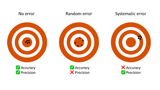
When you only have random error, if you measure the same thing multiple times, your measurements will tend to cluster or vary around the true value. Some values will be higher than the true score, while others will be lower. When you average out these measurements, you’ll get very close to the true score.
For this reason, random error isn’t considered a big problem when you’re collecting data from a large sample—the errors in different directions will cancel each other out when you calculate descriptive statistics. But it could affect the precision of your dataset when you have a small sample.
Systematic errors are much more problematic than random errors because they can skew your data to lead you to false conclusions. If you have systematic error, your measurements will be biased away from the true values. Ultimately, you might make a false positive or a false negative conclusion (a Type I or II error) about the relationship between the variables you’re studying.
Random error
Random error affects your measurements in unpredictable ways: your measurements are equally likely to be higher or lower than the true values.
In the graph below, the black line represents a perfect match between the true scores and observed scores of a scale. In an ideal world, all of your data would fall on exactly that line. The green dots represent the actual observed scores for each measurement with random error added.
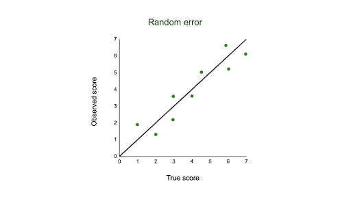
Random error is referred to as “noise”, because it blurs the true value (or the “signal”) of what’s being measured. Keeping random error low helps you collect precise data.
Sources of random errors
Some common sources of random error include:
- natural variations in real world or experimental contexts.
- imprecise or unreliable measurement instruments.
- individual differences between participants or units.
- poorly controlled experimental procedures.
| Random error source | Example |
|---|---|
| Natural variations in context | In an experiment about memory capacity, your participants are scheduled for memory tests at different times of day. However, some participants tend to perform better in the morning while others perform better later in the day, so your measurements do not reflect the true extent of memory capacity for each individual. |
| Imprecise instrument | You measure wrist circumference using a tape measure. But your tape measure is only accurate to the nearest half-centimeter, so you round each measurement up or down when you record data. |
| Individual differences | You ask participants to administer a safe electric shock to themselves and rate their pain level on a 7-point rating scale. Because pain is subjective, it’s hard to reliably measure. Some participants overstate their levels of pain, while others understate their levels of pain. |
What can proofreading do for your paper?
Scribbr editors not only correct grammar and spelling mistakes, but also strengthen your writing by making sure your paper is free of vague language, redundant words, and awkward phrasing.

See editing example
Reducing random error
Random error is almost always present in research, even in highly controlled settings. While you can’t eradicate it completely, you can reduce random error using the following methods.
Take repeated measurements
A simple way to increase precision is by taking repeated measurements and using their average. For example, you might measure the wrist circumference of a participant three times and get slightly different lengths each time. Taking the mean of the three measurements, instead of using just one, brings you much closer to the true value.
Increase your sample size
Large samples have less random error than small samples. That’s because the errors in different directions cancel each other out more efficiently when you have more data points. Collecting data from a large sample increases precision and statistical power.
Control variables
In controlled experiments, you should carefully control any extraneous variables that could impact your measurements. These should be controlled for all participants so that you remove key sources of random error across the board.
Systematic error
Systematic error means that your measurements of the same thing will vary in predictable ways: every measurement will differ from the true measurement in the same direction, and even by the same amount in some cases.
Systematic error is also referred to as bias because your data is skewed in standardized ways that hide the true values. This may lead to inaccurate conclusions.
Types of systematic errors
Offset errors and scale factor errors are two quantifiable types of systematic error.
An offset error occurs when a scale isn’t calibrated to a correct zero point. It’s also called an additive error or a zero-setting error.
A scale factor error is when measurements consistently differ from the true value proportionally (e.g., by 10%). It’s also referred to as a correlational systematic error or a multiplier error.
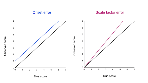
You can plot offset errors and scale factor errors in graphs to identify their differences. In the graphs below, the black line shows when your observed value is the exact true value, and there is no random error.
The blue line is an offset error: it shifts all of your observed values upwards or downwards by a fixed amount (here, it’s one additional unit).
The pink line is a scale factor error: all of your observed values are multiplied by a factor—all values are shifted in the same direction by the same proportion, but by different absolute amounts.
Sources of systematic errors
The sources of systematic error can range from your research materials to your data collection procedures and to your analysis techniques. This isn’t an exhaustive list of systematic error sources, because they can come from all aspects of research.
Response bias occurs when your research materials (e.g., questionnaires) prompt participants to answer or act in inauthentic ways through leading questions. For example, social desirability bias can lead participants try to conform to societal norms, even if that’s not how they truly feel.
Your question states: “Experts believe that only systematic actions can reduce the effects of climate change. Do you agree that individual actions are pointless?”
By citing “expert opinions,” this type of loaded question signals to participants that they should agree with the opinion or risk seeming ignorant. Participants may reluctantly respond that they agree with the statement even when they don’t.
Experimenter drift occurs when observers become fatigued, bored, or less motivated after long periods of data collection or coding, and they slowly depart from using standardized procedures in identifiable ways.
Initially, you code all subtle and obvious behaviors that fit your criteria as cooperative. But after spending days on this task, you only code extremely obviously helpful actions as cooperative.
You gradually move away from the original standard criteria for coding data, and your measurements become less reliable.
Sampling bias occurs when some members of a population are more likely to be included in your study than others. It reduces the generalizability of your findings, because your sample isn’t representative of the whole population.
Reducing systematic error
You can reduce systematic errors by implementing these methods in your study.
Triangulation
Triangulation means using multiple techniques to record observations so that you’re not relying on only one instrument or method.
For example, if you’re measuring stress levels, you can use survey responses, physiological recordings, and reaction times as indicators. You can check whether all three of these measurements converge or overlap to make sure that your results don’t depend on the exact instrument used.
Regular calibration
Calibrating an instrument means comparing what the instrument records with the true value of a known, standard quantity. Regularly calibrating your instrument with an accurate reference helps reduce the likelihood of systematic errors affecting your study.
You can also calibrate observers or researchers in terms of how they code or record data. Use standard protocols and routine checks to avoid experimenter drift.
Randomization
Probability sampling methods help ensure that your sample doesn’t systematically differ from the population.
In addition, if you’re doing an experiment, use random assignment to place participants into different treatment conditions. This helps counter bias by balancing participant characteristics across groups.
Masking
Wherever possible, you should hide the condition assignment from participants and researchers through masking (blinding).
Participants’ behaviors or responses can be influenced by experimenter expectancies and demand characteristics in the environment, so controlling these will help you reduce systematic bias.
Frequently asked questions about random and systematic error
-
What’s the difference between random and systematic error?
-
Random and systematic error are two types of measurement error.
Random error is a chance difference between the observed and true values of something (e.g., a researcher misreading a weighing scale records an incorrect measurement).
Systematic error is a consistent or proportional difference between the observed and true values of something (e.g., a miscalibrated scale consistently records weights as higher than they actually are).
-
Is random error or systematic error worse?
-
Systematic error is generally a bigger problem in research.
With random error, multiple measurements will tend to cluster around the true value. When you’re collecting data from a large sample, the errors in different directions will cancel each other out.
Systematic errors are much more problematic because they can skew your data away from the true value. This can lead you to false conclusions (Type I and II errors) about the relationship between the variables you’re studying.
Cite this Scribbr article
If you want to cite this source, you can copy and paste the citation or click the “Cite this Scribbr article” button to automatically add the citation to our free Citation Generator.
Bhandari, P.
(2022, December 05). Random vs. Systematic Error | Definition & Examples. Scribbr.
Retrieved February 9, 2023,
from https://www.scribbr.com/methodology/random-vs-systematic-error/
Is this article helpful?
You have already voted. Thanks 
Your vote is saved
Processing your vote…
: an error that is not determined by chance but is introduced by an inaccuracy (as of observation or measurement) inherent in the system

Example Sentences
Recent Examples on the Web
This kind of controversy comes down to very particular aspects of data collection, analysis, and sources of systematic error.
— Sean Carroll, Discover Magazine, 20 Apr. 2012
The polls could be off by another 2-3 points, due to a systematic error in turnout assumptions, putting Biden in reality just 4-5 points ahead of Trump instead of 9.
—Damon Linker, TheWeek, 30 Oct. 2020
So those voters were denied the ability to vote remotely, but that was due to systematic errors in ballot distribution, not directly via Supreme Court action.
—Eric Litke, USA TODAY, 11 Apr. 2020
Cognitive biases refer to a range of systematic errors in human decision-making stemming from the tendency to use mental shortcuts.
—Andrew R. Olenski, New York Times, 20 Feb. 2020
These example sentences are selected automatically from various online news sources to reflect current usage of the word ‘systematic error.’ Views expressed in the examples do not represent the opinion of Merriam-Webster or its editors. Send us feedback.
Word History
First Known Use
1826, in the meaning defined above
Time Traveler
The first known use of systematic error was
in 1826
Dictionary Entries Near systematic error
Cite this Entry
“Systematic error.” Merriam-Webster.com Dictionary, Merriam-Webster, https://www.merriam-webster.com/dictionary/systematic%20error. Accessed 9 Feb. 2023.
Share
More from Merriam-Webster on systematic error
Last Updated:
2 Jan 2023
— Updated example sentences
Subscribe to America’s largest dictionary and get thousands more definitions and advanced search—ad free!
Merriam-Webster unabridged
The most significant difference between the random and the systematic error is that the random error occurs because of the unpredictable disturbances caused by the unknown source or because of the limitation of the instrument. Whereas, the systematic error occurs because of the imperfection of the apparatus. The other differences between the random and the systematic error are represented below in the comparison chart.
The systematic error occurs because of the imperfection of the apparatus. Hence the measured value is either very high or very low as compared to the true value. While in random error the magnitude of error changes in every reading.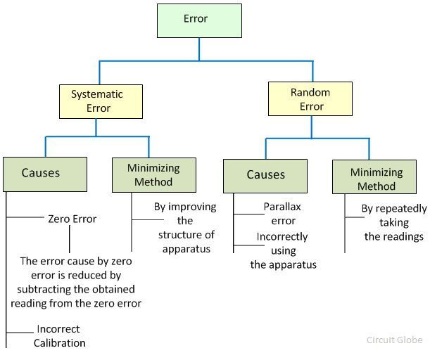
The complete elimination of both the errors cannot be possible. The errors can only be reduced by using the particular methods. The random error reduces by repeatedly taking the readings. And the systematic error reduces by improving the mechanical structure of the apparatus.
Content: Random Vs Systematic Error
- Comparison Chart
- Definition
- Key Differences
- Conclusion
| Basis For Comparison | Random Error | Systematic Error |
|---|---|---|
| Definition | The random error occurs in the experiment because of the uncertain changes in the environment. | It is a constant error which remains same for all the measurements. |
| Causes | Environment, limitation of the instrument, etc. | Incorrect calibration and incorrectly using the apparatus |
| Minimize | By repeatedly taking the reading. | By improving the design of the apparatus. |
| Magnitude of Error | Vary | Constant |
| Direction of Error | Occur in both the direction. | Occur only in one direction. |
| Types | Do not have | Three (Instrument, Environment and systematic error) |
| Reproducible | Non-reproducible | Reproducible |
Definition of Random Error
The uncertain disturbances occur in the experiment is known as the random errors. Such type of errors remains in the experiment even after the removal of the systematic error. The magnitude of error varies from one reading to another. The random errors are inconsistent and occur in both the directions.
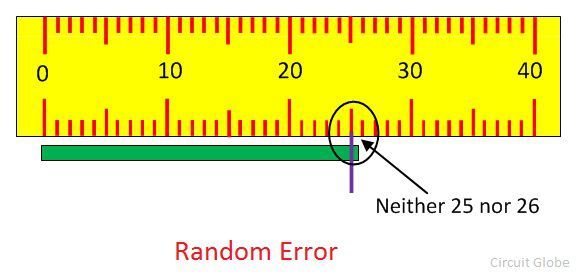
The presence of random errors is determined only when the different readings are obtained for the measurement of the same quantity under the same condition.
Definition of Systematic Error
The constant error occurs in the experiment because of the imperfection of the mechanical structure of the apparatus is known as the systematic error. The systematic errors arise because of the incorrect calibration of the device.
The error is mainly categorised into three types.
- Instrumental Error
- Environmental Error
- Observational Error
Instrumental Error – The instrumental error occurs because of the three reasons.
- Misuse of the apparatus.
- Imperfection in the mechanical structure of the apparatus.
- The error occurs because of the loading effect.
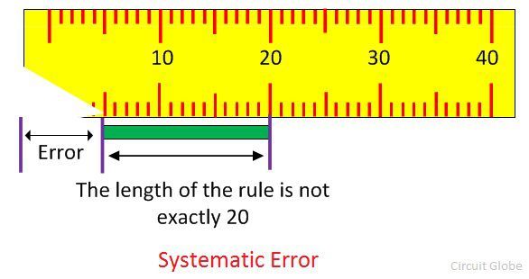
Observational Error – The error occurs in the observation of the reading is known as the observational error. For example, consider the pointer of voltmeter rest on the surface of the scale. The observational error occurs in the reading if the line of vision is exactly not above the pointer.
Environmental Error – Such types of error occurs because of the changes in the surroundings condition like humidity, pressure, magnetic or electrostatic field, etc. The experimental errors can be reduced by making some arrangements in the laboratory for controlling the temperature and humidity. Also, before experimenting make ensure that there should be no magnetic and electric field.
Key Differences between the Random & Systematic Error
The following are the major differences between the systematic and random error.
- The random error means the unpredictable disturbance occurs in the experiment by the unknown source. Whereas, the systematic error occurs because of the inbuilt defect of the apparatus.
- The random error occurs in both the direction, whereas the systematic error occurs only in one direction. The systematic errors arise because of the inbuilt fault of the apparatus, hence it always gives the same error. The random error occurs because of the unknown source, thereby occurs in any direction.
- The magnitude of systematic error remains constant because the defect is inbuilt inside the apparatus. Whereas, the magnitude of the random error is variable.
- The zero error and the incorrect calibration of apparatus cause the systematic error. The random error is because of the parallax or by incorrectly using the apparatus.
- The random error reduces by taking the two or more readings of the same experiment, whereas the systematic error reduces by carefully designing the apparatus.
- The random error does not have any specific types, whereas the systematic error is categorised into three types, i.e., instrument error, environment error and systematic error.
- The random error is non-reproducible whereas the systematic error is reproducible because the defect is inbuilt with the apparatus.
Conclusion
The random error happens because of any disturbances occurs in the surrounding like the variation in temperature, pressure or because of the observer who takes the wrong reading. The systematic error arises because of the mechanical structure of the apparatus. The complete elimination of both the error is impossible.
Systematic errors are biases in measurement which lead to the situation where the mean of many separate measurements differs significantly from the actual value of the measured attribute. All measurements are prone to systematic errors, often of several different types. Sources of systematic error may be imperfect calibration of measurement instruments (zero error), changes in the environment which interfere with the measurement process and sometimes imperfect methods of observation can be either zero error or percentage error. For example, consider an experimenter taking a reading of the time period of a pendulum swinging past a fiducial mark: If his stop-watch or timer starts with 1 second on the clock then all of his results will be off by 1 second (zero error). If the experimenter repeats this experiment twenty times (starting at 1 second each time), then there will be a percentage error in the calculated average of his results; the final result will be slightly larger than the true period. Distance measured by radar will be systematically overestimated if the slight slowing down of the waves in air is not accounted for. Incorrect zeroing of an instrument leading to a zero error is an example of systematic error in instrumentation.
Systematic errors may also be present in the result of an estimate based on a mathematical model or physical law. For instance, the estimated oscillation frequency of a pendulum will be systematically in error if slight movement of the support is not accounted for.
Systematic errors can be either constant, or be related (e.g. proportional or a percentage) to the actual value of the measured quantity, or even to the value of a different quantity (the reading of a ruler can be affected by environment temperature). When they are constant, they are simply due to incorrect zeroing of the instrument. When they are not constant, they can change sign. For instance, if a thermometer is affected by a proportional systematic error equal to 2% of the actual temperature, and the actual temperature is 200°, 0°, or −100°, the measured temperature will be 204° (systematic error = +4°), 0° (null systematic error) or −102° (systematic error = −2°), respectively. Thus, the temperature will be overestimated when it will be above zero, and underestimated when it will be below zero.
Constant systematic errors are very difficult to deal with, because their effects are only observable if they can be removed. Such errors cannot be removed by repeating measurements or averaging large numbers of results. A common method to remove systematic error is through calibration of the measurement instrument.
In a statistical context, the term systematic error usually arises where the sizes and directions of possible errors are unknown.
Drift
Systematic errors which change during an experiment (drift) are easier to detect. Measurements show trends with time rather than varying randomly about a mean.
Drift is evident if a measurement of a constant quantity is repeated several times and the measurements drift one way during the experiment, for example if each measurement is higher than the previous measurement which could perhaps occur if an instrument becomes warmer during the experiment. If the measured quantity is variable, it is possible to detect a drift by checking the zero reading during the experiment as well as at the start of the experiment (indeed, the zero reading is a measurement of a constant quantity). If the zero reading is consistently above or below zero, a systematic error is present. If this cannot be eliminated, for instance by resetting the instrument immediately before the experiment, it needs to be allowed for by subtracting its (possibly time-varying) value from the readings, and by taking it into account in assessing the accuracy of the measurement.
If no pattern in a series of repeated measurements is evident, the presence of fixed systematic errors can only be found if the measurements are checked, either by measuring a known quantity or by comparing the readings with readings made using a different apparatus, known to be more accurate. For example, suppose the timing of a pendulum using an accurate stopwatch several times gives readings randomly distributed about the mean. A systematic error is present if the stopwatch is checked against the ‘speaking clock’ of the telephone system and found to be running slow or fast. Clearly, the pendulum timings need to be corrected according to how fast or slow the stopwatch was found to be running. Measuring instruments such as ammeters and voltmeters need to be checked periodically against known standards.
Systematic errors can also be detected by measuring already known quantities. For example, a spectrometer fitted with a diffraction grating may be checked by using it to measure the wavelength of the D-lines of the sodium electromagnetic spectrum which are at 600nm and 589.6 nm. The measurements may be used to determine the number of lines per millimetre of the diffraction grating, which can then be used to measure the wavelength of any other spectral line.
Systematic versus random error
Measurement errors can be divided into two components: random error and systematic error.[1] Random error is always present in a measurement. It is caused by inherently unpredictable fluctuations in the readings of a measurement apparatus or in the experimenter’s interpretation of the instrumental reading. Random errors show up as different results for ostensibly the same repeated measurement. Systematic error cannot be discovered this way because it always pushes the results in the same direction. If the cause of a systematic error can be identified, then it can usually be eliminated.
See also
- Experimental uncertainty analysis
- Biased sample
- Errors and residuals in statistics
- Observational error
References
- ^ John Robert Taylor (1999). An Introduction to Error Analysis: The Study of Uncertainties in Physical Measurements. University Science Books. p. 94, §4.1. ISBN 093570275X. http://books.google.com/books?id=giFQcZub80oC&pg=PA94.
No matter how careful you are when conducting experiments, there will likely be an experimental error. Whether through the challenges inherent taking the measurements accurately or problems with your equipment, avoiding error altogether is next to impossible. To counteract this issue, scientists do their best to categorize errors and quantify any uncertainty in measurements they make. Finding out the difference between systematic and random errors is a key part of learning to design better experiments and to minimize any errors that do creep through.
TL;DR (Too Long; Didn’t Read)
Systematic errors usually result from equipment that isn’t correctly calibrated. Every measurement you take will be wrong by the same amount because there is a problem with your measuring device. Random errors are unavoidable and result from difficulties taking measurements or attempting to measure quantities that vary with time. These errors will fluctuate but generally cluster around the true value.
What Is Random Error?
Random error describes errors that fluctuate due to the unpredictability or uncertainty inherent in your measuring process, or the variation in the quantity you’re trying to measure.
A scientist measuring an insect, for example, would try to position the insect at the zero point of a ruler or measuring stick, and read the value at the other end. The ruler itself will probably only measure down to the nearest millimeter, and reading this with precision can be difficult. You may underestimate the true size of the insect or overestimate it, based on how well you read the scale and your judgment as to where the head of the insect stops. The insect might also move ever so slightly from the zero position without you realizing. Repeating the measurement multiple times yields many different results because of this, but they would likely cluster around the true value.
Similarly, taking measurements of a quantity that changes from moment to moment leads to random error. Wind speed, for example, may pick up and fall off at different points in time. If you take a measurement one minute, it probably won’t be exactly the same a minute later. Again, repeated measurements will lead to results that fluctuate but cluster around the true value.
What Is Systematic Error?
A systematic error is one that results from a persistent issue and leads to a consistent error in your measurements. For example, if your measuring tape has been stretched out, your results will always be lower than the true value. Similarly, if you’re using scales that haven’t been set to zero beforehand, there will be a systematic error resulting from the mistake in the calibration (e.g., if a true weight of 0 reads as 5 grams, 10 grams will read as 15 and 15 grams will read as 20).
Other Differences Between Systematic and Random Errors
The main difference between systematic and random errors is that random errors lead to fluctuations around the true value as a result of difficulty taking measurements, whereas systematic errors lead to predictable and consistent departures from the true value due to problems with the calibration of your equipment. This leads to two extra differences that are worth noting.
Random errors are essentially unavoidable, while systematic errors are not. Scientists can’t take perfect measurements, no matter how skilled they are. If the quantity you’re measuring varies from moment to moment, you can’t make it stop changing while you take the measurement, and no matter how detailed your scale, reading it accurately still poses a challenge. The good news is that repeating your measurement multiple times and taking the average effectively minimizes this issue.
Systematic errors may be difficult to spot. This is because everything you measure will be wrong by the same (or a similar) amount and you may not realize there is an issue at all. However, unlike random errors they can often be avoided altogether. Calibrate your equipment properly prior to using it, and systematic errors will be much less likely.
«Systematic bias» redirects here. For the sociological and organizational phenomenon, see Systemic bias.
Observational error (or measurement error) is the difference between a measured value of a quantity and its true value.[1] In statistics, an error is not necessarily a «mistake». Variability is an inherent part of the results of measurements and of the measurement process.
Measurement errors can be divided into two components: random and systematic.[2]Random errors are errors in measurement that lead to measurable values being inconsistent when repeated measurements of a constant attribute or quantity are taken. Systematic errors are errors that are not determined by chance but are introduced by repeatable processes inherent to the system.[3] Systematic error may also refer to an error with a non-zero mean, the effect of which is not reduced when observations are averaged.[citation needed]
Measurement errors can be summarized in terms of accuracy and precision.
Measurement error should not be confused with measurement uncertainty.
Science and experimentsEdit
When either randomness or uncertainty modeled by probability theory is attributed to such errors, they are «errors» in the sense in which that term is used in statistics; see errors and residuals in statistics.
Every time we repeat a measurement with a sensitive instrument, we obtain slightly different results. The common statistical model used is that the error has two additive parts:
- Systematic error which always occurs, with the same value, when we use the instrument in the same way and in the same case.
- Random error which may vary from observation to another.
Systematic error is sometimes called statistical bias. It may often be reduced with standardized procedures. Part of the learning process in the various sciences is learning how to use standard instruments and protocols so as to minimize systematic error.
Random error (or random variation) is due to factors that cannot or will not be controlled. One possible reason to forgo controlling for these random errors is that it may be too expensive to control them each time the experiment is conducted or the measurements are made. Other reasons may be that whatever we are trying to measure is changing in time (see dynamic models), or is fundamentally probabilistic (as is the case in quantum mechanics — see Measurement in quantum mechanics). Random error often occurs when instruments are pushed to the extremes of their operating limits. For example, it is common for digital balances to exhibit random error in their least significant digit. Three measurements of a single object might read something like 0.9111g, 0.9110g, and 0.9112g.
CharacterizationEdit
Measurement errors can be divided into two components: random error and systematic error.[2]
Random error is always present in a measurement. It is caused by inherently unpredictable fluctuations in the readings of a measurement apparatus or in the experimenter’s interpretation of the instrumental reading. Random errors show up as different results for ostensibly the same repeated measurement. They can be estimated by comparing multiple measurements and reduced by averaging multiple measurements.
Systematic error is predictable and typically constant or proportional to the true value. If the cause of the systematic error can be identified, then it usually can be eliminated. Systematic errors are caused by imperfect calibration of measurement instruments or imperfect methods of observation, or interference of the environment with the measurement process, and always affect the results of an experiment in a predictable direction. Incorrect zeroing of an instrument leading to a zero error is an example of systematic error in instrumentation.
The Performance Test Standard PTC 19.1-2005 “Test Uncertainty”, published by the American Society of Mechanical Engineers (ASME), discusses systematic and random errors in considerable detail. In fact, it conceptualizes its basic uncertainty categories in these terms.
Random error can be caused by unpredictable fluctuations in the readings of a measurement apparatus, or in the experimenter’s interpretation of the instrumental reading; these fluctuations may be in part due to interference of the environment with the measurement process. The concept of random error is closely related to the concept of precision. The higher the precision of a measurement instrument, the smaller the variability (standard deviation) of the fluctuations in its readings.
SourcesEdit
Sources of systematic errorEdit
Imperfect calibrationEdit
Sources of systematic error may be imperfect calibration of measurement instruments (zero error), changes in the environment which interfere with the measurement process and sometimes imperfect methods of observation can be either zero error or percentage error. If you consider an experimenter taking a reading of the time period of a pendulum swinging past a fiducial marker: If their stop-watch or timer starts with 1 second on the clock then all of their results will be off by 1 second (zero error). If the experimenter repeats this experiment twenty times (starting at 1 second each time), then there will be a percentage error in the calculated average of their results; the final result will be slightly larger than the true period.
Distance measured by radar will be systematically overestimated if the slight slowing down of the waves in air is not accounted for. Incorrect zeroing of an instrument leading to a zero error is an example of systematic error in instrumentation.
Systematic errors may also be present in the result of an estimate based upon a mathematical model or physical law. For instance, the estimated oscillation frequency of a pendulum will be systematically in error if slight movement of the support is not accounted for.
QuantityEdit
Systematic errors can be either constant, or related (e.g. proportional or a percentage) to the actual value of the measured quantity, or even to the value of a different quantity (the reading of a ruler can be affected by environmental temperature). When it is constant, it is simply due to incorrect zeroing of the instrument. When it is not constant, it can change its sign. For instance, if a thermometer is affected by a proportional systematic error equal to 2% of the actual temperature, and the actual temperature is 200°, 0°, or −100°, the measured temperature will be 204° (systematic error = +4°), 0° (null systematic error) or −102° (systematic error = −2°), respectively. Thus the temperature will be overestimated when it will be above zero and underestimated when it will be below zero.
DriftEdit
Systematic errors which change during an experiment (drift) are easier to detect. Measurements indicate trends with time rather than varying randomly about a mean. Drift is evident if a measurement of a constant quantity is repeated several times and the measurements drift one way during the experiment. If the next measurement is higher than the previous measurement as may occur if an instrument becomes warmer during the experiment then the measured quantity is variable and it is possible to detect a drift by checking the zero reading during the experiment as well as at the start of the experiment (indeed, the zero reading is a measurement of a constant quantity). If the zero reading is consistently above or below zero, a systematic error is present. If this cannot be eliminated, potentially by resetting the instrument immediately before the experiment then it needs to be allowed by subtracting its (possibly time-varying) value from the readings, and by taking it into account while assessing the accuracy of the measurement.
If no pattern in a series of repeated measurements is evident, the presence of fixed systematic errors can only be found if the measurements are checked, either by measuring a known quantity or by comparing the readings with readings made using a different apparatus, known to be more accurate. For example, if you think of the timing of a pendulum using an accurate stopwatch several times you are given readings randomly distributed about the mean. Hopings systematic error is present if the stopwatch is checked against the ‘speaking clock’ of the telephone system and found to be running slow or fast. Clearly, the pendulum timings need to be corrected according to how fast or slow the stopwatch was found to be running.
Measuring instruments such as ammeters and voltmeters need to be checked periodically against known standards.
Systematic errors can also be detected by measuring already known quantities. For example, a spectrometer fitted with a diffraction grating may be checked by using it to measure the wavelength of the D-lines of the sodium electromagnetic spectrum which are at 600 nm and 589.6 nm. The measurements may be used to determine the number of lines per millimetre of the diffraction grating, which can then be used to measure the wavelength of any other spectral line.
Constant systematic errors are very difficult to deal with as their effects are only observable if they can be removed. Such errors cannot be removed by repeating measurements or averaging large numbers of results. A common method to remove systematic error is through calibration of the measurement instrument.
Sources of random errorEdit
The random or stochastic error in a measurement is the error that is random from one measurement to the next. Stochastic errors tend to be normally distributed when the stochastic error is the sum of many independent random errors because of the central limit theorem. Stochastic errors added to a regression equation account for the variation in Y that cannot be explained by the included Xs.
SurveysEdit
The term «observational error» is also sometimes used to refer to response errors and some other types of non-sampling error.[1] In survey-type situations, these errors can be mistakes in the collection of data, including both the incorrect recording of a response and the correct recording of a respondent’s inaccurate response. These sources of non-sampling error are discussed in Salant and Dillman (1994) and Bland and Altman (1996).[4][5]
These errors can be random or systematic. Random errors are caused by unintended mistakes by respondents, interviewers and/or coders. Systematic error can occur if there is a systematic reaction of the respondents to the method used to formulate the survey question. Thus, the exact formulation of a survey question is crucial, since it affects the level of measurement error.[6] Different tools are available for the researchers to help them decide about this exact formulation of their questions, for instance estimating the quality of a question using MTMM experiments. This information about the quality can also be used in order to correct for measurement error.[7][8]
Effect on regression analysisEdit
If the dependent variable in a regression is measured with error, regression analysis and associated hypothesis testing are unaffected, except that the R2 will be lower than it would be with perfect measurement.
However, if one or more independent variables is measured with error, then the regression coefficients and standard hypothesis tests are invalid.[9]: p. 187 This is known as attenuation bias.[10]
See alsoEdit
- Bias (statistics)
- Cognitive bias
- Correction for measurement error (for Pearson correlations)
- Errors and residuals in statistics
- Error
- Replication (statistics)
- Statistical theory
- Metrology
- Regression dilution
- Test method
- Propagation of uncertainty
- Instrument error
- Measurement uncertainty
- Errors-in-variables models
- Systemic bias
ReferencesEdit
- ^ a b Dodge, Y. (2003) The Oxford Dictionary of Statistical Terms, OUP. ISBN 978-0-19-920613-1
- ^ a b John Robert Taylor (1999). An Introduction to Error Analysis: The Study of Uncertainties in Physical Measurements. University Science Books. p. 94, §4.1. ISBN 978-0-935702-75-0.
- ^ «Systematic error». Merriam-webster.com. Retrieved 2016-09-10.
- ^ Salant, P.; Dillman, D. A. (1994). How to conduct your survey. New York: John Wiley & Sons. ISBN 0-471-01273-4.
- ^ Bland, J. Martin; Altman, Douglas G. (1996). «Statistics Notes: Measurement Error». BMJ. 313 (7059): 744. doi:10.1136/bmj.313.7059.744. PMC 2352101. PMID 8819450.
- ^ Saris, W. E.; Gallhofer, I. N. (2014). Design, Evaluation and Analysis of Questionnaires for Survey Research (Second ed.). Hoboken: Wiley. ISBN 978-1-118-63461-5.
- ^ DeCastellarnau, A. and Saris, W. E. (2014). A simple procedure to correct for measurement errors in survey research. European Social Survey Education Net (ESS EduNet). Available at: http://essedunet.nsd.uib.no/cms/topics/measurement Archived 2019-09-15 at the Wayback Machine
- ^ Saris, W. E.; Revilla, M. (2015). «Correction for measurement errors in survey research: necessary and possible» (PDF). Social Indicators Research. 127 (3): 1005–1020. doi:10.1007/s11205-015-1002-x. hdl:10230/28341. S2CID 146550566.
- ^ Hayashi, Fumio (2000). Econometrics. Princeton University Press. ISBN 978-0-691-01018-2.
- ^ Angrist, Joshua David; Pischke, Jörn-Steffen (2015). Mastering ‘metrics : the path from cause to effect. Princeton, New Jersey. p. 221. ISBN 978-0-691-15283-7. OCLC 877846199.
The bias generated by this sort of measurement error in regressors is called attenuation bias.
Further readingEdit
- Cochran, W. G. (1968). «Errors of Measurement in Statistics». Technometrics. 10 (4): 637–666. doi:10.2307/1267450. JSTOR 1267450.