Реферат Отчет 38 с., 3 главы, 22 рис., 2 табл., 16 источников, 4 прил видео стеганография, стеганография mpeg, сокрытие информации в видео, встраивание и извлечение информации, дискретное косинусное преобразование, помехоустойчивое кодирование, циклические
Построение таблицы синдромов ошибок
|
Скачать 318,6 Kb.
|


- Навигация по данной странице:
- Декодирование и исправление ошибок
Построение таблицы синдромов ошибок
Перед тем как начать декодирование, необходимо построить таблицу синдромов ошибок, с помощью которой будет происходить исправление ошибок. Для этого нужно знать количество ошибок, которое двоичный циклический  -код может исправлять. Количество исправляемых ошибок
  для двоичного циклического -кода рассчитывается по следующей формуле.

где — количество исправляемых ошибок,
 – минимальное кодовое расстояние.
Минимальное кодовое расстояние  для двоичного циклического -кода рассчитывается как минимальный вес среди его всех ненулевых кодовых слов. Весом кодового слова является количество единичных бит в этом слове. Для двоичного циклического (7,4)-кода существует всего
  кодовых слов (табл. 1). Для этого кода минимальное кодовое расстояние
  . Подставляя это значение в формулу (1.3), получаем что, двоичный циклический (7,4)-код исправляет одну ошибку.
Таблица 1.1
Кодовые слова двоичного циклического (7,4)-кода ( )
)
|
0000000 |
0100111 |
1000101 |
1100010 |
|
0001011 |
0101100 |
1001110 |
1101001 |
|
0010110 |
0110001 |
1010011 |
1110100 |
|
0011101 |
0111010 |
1011000 |
1111111 |
Так как двоичный циклический (7,4)-код исправляет всего одну ошибку, то общее количество многочленов ошибок равно длине кодового слова  . Для каждого многочлена ошибки находится его синдром, остаток от деления на порождающий многочлен
  (табл. 1.2).
Таблица 1.2
Синдромы однократных ошибок двоичного циклического (7,4)-кода с порождающим многочленом .
|
Ошибка |
Синдром |
|
0000001 |
001 |
|
0000010 |
010 |
|
0000100 |
100 |
|
0001000 |
011 |
|
0010000 |
110 |
|
0100000 |
111 |
|
1000000 |
101 |
Декодирование и исправление ошибок
Декодирование двоичного циклического -кода с порождающим многочленом происходит по следующим шагам [15, гл. 3.8]:
-
Вычисляется синдром ошибки с помощью алгоритма деления Евклида, описанном в 1.2.1.1.
-
Если синдром нулевой, то кодовое слово не содержит ошибок. Если синдром ненулевой, то определятся ошибочный бит с помощью таблицы синдромов и исправляется.
-
Так как кодирование систематическое, то можно просто отсечь проверочную часть длины и получить декодированное информационное слово.
 и получить декодированное информационное слово.
Ниже представлен пример декодирования кодового слова (0010011) с помощью двоичного циклического (7,4)-кода с порождающим многочленом .
-
Находим остаток от деления (синдром ошибки) с помощью алгоритма деления Евклида
0
0
1
0
0
1
1
=
0
0
1
0
1
1
0
=
1
0
1
=
-
Синдром не равен нулю, поэтому находим синдром в таблице синдромов (табл. 1.2) и соответствующий ему ошибочный бит (1000000).
-
Исправляем ошибочный бит и получаем правильное кодовое слово (1010011). Отсекаем проверочную часть и получаем информационное слово (1010).


-
Каталог: data -> 2014
2014 -> Программа дисциплины для направления/ специальности подготовки бакалавра/ магистра/ специалиста
2014 -> «Особенности реализации личностно-ориентированного подхода в профессиональной подготовке студентов высших учебных заведений»
2014 -> Программа «Управление образованием»
2014 -> Кадровая политика вуза
2014 -> Баврина Анна Петровна профессиональная мотивация преподавателей вуза (на примере нгма) Выпускная квалификационная работа по направлению 080200. 68 «Менеджмент» магистранта группы №12учр
2014 -> «Российское общество эпохи реформ Александра ii»
2014 -> «Корпоративная культура средств массовой информации на примере телеканала рен тв»
2014 -> Начиная с восьмидесятых годов двадцатого века тема корпоративной или организационной культуры стала одной из центральных в управленческой литературе. Все больше исследователей посвящают этому феномену свои научные труды
2014 -> Система методического сопровождения педагогов по формированию метапредметных результатов в условиях подготовки и введения Федеральных государственных образовательных стандартовСкачать 318,6 Kb.
Поделитесь с Вашими друзьями:

Принцип синдромного
декодирования рассмотрим на примере
несложного
блокового кода.
Пример 5.3.
Синдромный
декодер систематического кода (7, 4).
В
соответствии с правилом вычисления
синдрома (5.8) для реализации синдромного
декодера необходимо сформировать
транспонированную проверочную матрицу
кода (7, 4). Проверочная матрица этого
кода имеет вид (5.5). Применяя к ней правило
транспонирования матриц, получаем:
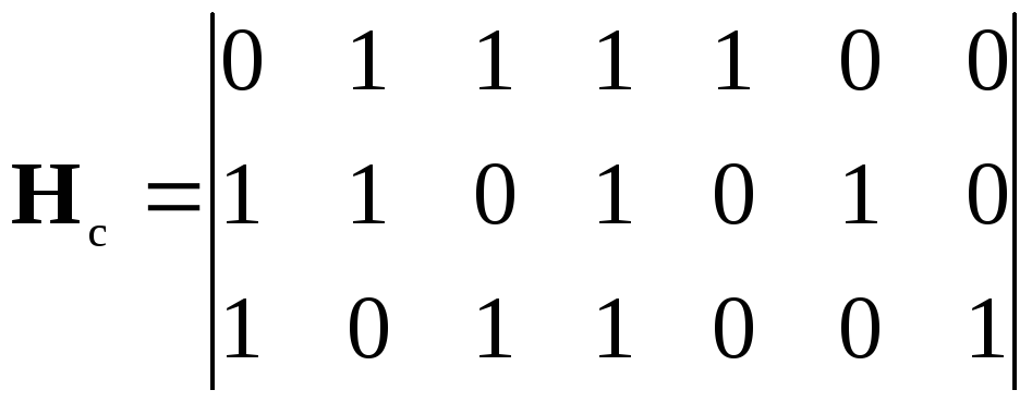 ,
,
 . (5.9)
Если в канале связи
действуют однократные ошибки, то векторы
ошибок удобно записывать так:
e1 = (1000000),
e2 = (0100000),
e3 = (0010000),
…, en = (0000001). (5.10)
В такой
записи вектор ошибки
ei
представляет набор n
символов, в котором на месте с номером
i (счет
слева) расположен символ ошибки 1, а на
остальных местах расположены нулевые
символы.
векторы
ошибки могут быть представлены в виде
единичной матрицы:
 , (5.11)
каждая
строка которой есть вектор
однократной ошибки.
Используя свойства единичных матриц,
нетрудно показать, что матрица синдромов
совпадает с транспонированной проверочной
матрицей этого кода (5.9):
S
= E·HT
= In·HT
= HT. (5.12)
|
При |
Это
является основанием для составления
таблицы
синдромов.
Ниже приведена табл. 5.1 синдромов для
кода (7,4), составленная по данным строк
транспонированной проверочной матрицы
(5.9). В таблице каждому
вектору ошибки соответствует свой
вектор синдрома,
указывающий местоположение ошибочного
символа в кодовой комбинации на
входе декодера.
таблица 5.1
–Таблица синдромов для декодирования
кода (7, 4)
|
Синдром |
011 |
110 |
101 |
111 |
100 |
010 |
001 |
|
Вектор |
e1 |
e2 |
e3 |
e4 |
e5 |
e6 |
e7 |
Это позволяет
сформулировать алгоритм синдромного
декодирования:
|
Алгоритм
1.
2.
3.
4.
5.
bi=
6. |
Структура синдромного
декодера кода (7, 4), реализующего этот
алгоритм, приведена на рис. 5.2.
В
соответствии с правилами формирования
синдромов (5.12) на сумматоры по модулю 2
подаются принимаемые из канала символы,
причем, связи с линиями канальных
символов имеются там, где в строках
транспонированной проверочной матрицы
расположен символ 1. В схеме анализатора
синдромов в соответствии с данными
табл. 5.1 происходит преобразование
векторов синдромов S = (s0,
s1,
…, sn–k–1)
в соответствующие им векторы ошибки e,
которые затем подаются на сумматоры
корректора ошибок. В результате сложения
вектора принятых из канала символов
с
соответствующими им векторами ошибки
e
происходит
исправление
канальных ошибок.

Соседние файлы в предмете [НЕСОРТИРОВАННОЕ]
- #
- #
- #
- #
- #
- #
- #
- #
- #
- #
- #
| 1. /Pomexoustoyxhiviye_kodi_vtelekom_sistemax.doc | Учебное пособие предназначено для бакалавров и магистров, изучающих вопросы помехоустойчивого кодирования, а также для специалистов по защите информации от ошибок |
Таблица 2.1
| Простой
четырех символьный код C(x) |
Образующий
полином P(x) |
Циклический
(7,4) код |
| 0000
0001 0010 0011 0100 0101 0110 0111 1000 1001 1010 1011 1100 1101 1110 1111 |
1101 |
0000000
0001101 0011010 0010111 0110100 0111001 0101110 0100011 1101000 1100101 1110010 1111111 1011100 1010001 1000110 1001011 |
2.4. Способы исправления ошибок на основе синдрома ошибок, свойства цикличности и анализ веса остатка
Синдром циклического кода, как и в любом систематическом коде, определяется суммой по модулю два, принятых проверочных элементов и элементов первичной группы, сформированных из принятых элементов информационной группы.
В циклическом коде для определения синдрома следует разделить приятую кодовую комбинацию на кодовую комбинацию производящего полинома. Если все элементы приняты без ошибок, остаток R(x) от деления равен нулю. Наличие ошибок приводит к тому, что остаток R(x)≠0.
Для определения номеров элементов, в которых произошла ошибка, существует несколько методов. Один из них основан на свойстве, которое заключается в том, что R(х), полученный при делении принятого многочлена H(x) на Pr(x), равен R(x), полученному в результате деления соответствующего многочлена ошибок E(x) на Pr(x).
Многочлен ошибок E(x)=A(x)+H(x) , где A(x)– исходный многочлен циклического кода. Так, если ошибка произошла в а1, то при коде (9.5) E1(0,1)=100000000, ошибка в а2 соответствует E2(0,1)=010000000 и т.д., остаток от деления E(0,1) на Pr(0,1)=10011=R1(0,1) для данного 9-элементного кода всегда одинаков, он не зависит от вида предаваемой комбинации. В рассматриваемом примере R(0,1)=0101. Наличие ошибки в других элементах (a2, a3, …) приведет к другим остаткам. Остатки зависят только от вида Pr(x) и n. Для n=9 и P4(0,1)=10011 будет следующее соответствие:
Таблица.2.2
| Элемент с ошибкой | a1 | a2 | a3 | a4 | a5 |
| Синдром | 0101 | 1011 | 1100 | 0110 | 0011 |
Указанное однозначное соответствие можно использовать для определения места ошибки. Синдром не зависит от переданной кодовой комбинации, но в нем сосредоточена вся информация о наличии ошибок. Обнаружение и исправление ошибок в систематических кодах может производиться только на основе анализа синдрома.
На основании приведенного свойства существует следующий метод определения места ошибки. Сначала определяется остаток R1(0,1), соответствующий наличию ошибки в старшем разряде. Если ошибка произошла в следующем разряде (более низком), то такой же остаток получится в произведении принятого многочлена и x, т.е. H(x)x. Это служит основанием для следующего приема, суть которого ясна из следующего примера.
Пример: Предположим, задан код (11,7) в виде кодовой комбинации 10110111100. Здесь последние четыре разряда проверочные и получены на основе использования производящего многочлена P(0,1)=100011. Принята кодовая комбинация 10111111100. Определить ошибочно принятый элемент.
Вычисляем R(x) как остаток от деления E(x)=10000000000 на 10011. Произведя деление, получим 0111. Далее делим принятую комбинацию на Pr(x) и получаем остаток R(0,1). Если R(0,1)=R1(0,1), то ошибка в старшем разряде. Если нет, то дописываем «0» и продолжаем деление. Номер ошибочно принятого разряда (отсчет слева направо) на единицу больше числа приписанных нулей, после которых остаток окажется равным 0111. Проведем процесс деления, отмечая штрихом получаемые остатки R1(0,1), R2(0,1), R3(0,1), R4(0,1):
 (2.6)
(2.6)
В данном примере для этого пришлось дописать четыре нуля. Это означает, что ошибка произошла в пятом элементе, т.е. исправленная кодовая комбинация будет имееть вид
![]() . (2.7)
. (2.7)
На основе свойства цикличности, предполагается, что ошибка произошла в старшем разряде. Определяется остаток, соответствующий вектору ошибок:
![]()
![]() (2.8)
(2.8)
если остатки совпадают, то ошибка произошла в старшем разряде; если не совпадают, то дописывается 0 в комбинацию R(x) и продолжается деление, пока остатки не совпадут.
Важным свойством циклических кодов является то, что все они строятся с помощью образующего полинома Р(х). приведем методику построения циклического кода. Образующий полином Р(х) принимает участие в образовании каждой кодовой комбинации, поэтому комбинация кода делится на образующий полином без остатка. Однако без остатка делятся только те многочлены (комбинации), которые принадлежат данному коду, т.е. образующий полином позволяет выбрать разрешенные кодовые комбинации из всех возможных. Если же при делении принятой кодовой комбинации циклического кода на образующий многочлен будет получен остаток, значит, имеет место ошибка. Таким образом, остатки от деления принятой комбинации на образующий полином являются опознавателями ошибок циклических кодов. Но данные остатки еще не указывают непосредственно на место ошибки в кодовой комбинации.
В циклических кодах идея исправления ошибок основывается на следующем: ошибочная комбинация после переделанного числа циклических сдвигов «подгоняется» под остаток таким образом, чтобы в сумме с остатком она давала бы исправленную комбинацию. Остаток при этом представляет собой разницу между искаженными и правильными символами, а единицы в остатке стоят на местах искаженных разрядов в «подогнанной» циклическими сдвигами комбинациями. «Подгоняют» искаженную комбинацию до тех пор, пока число единиц в остатке не будет равно числу ошибок в коде. При этом, естественно, число единиц может быть равно числу ошибок tи, исправляемых данным кодом (код исправляет три ошибки и в искаженной комбинации три ошибки) или меньше tи (код исправляет три ошибки, в принятой комбинации – одна ошибка).
Таким образом, для обнаружения и исправления ошибочного разряда производят следующие операции.
1) Принятую комбинацию делят на образующий полином;
2) Подсчитывают количество единиц в остатке (вес остатка). Если ![]()
где tи – допустимое число исправляемых данным кодом ошибок, принятую комбинацию складывают по модулю два с получением остатком. Сумма дает исправленную комбинацию. Если ![]() то
то
3) Производят циклический сдвиг принятой комбинации влево на один разряд. Комбинацию, полученную в результате циклического сдвига, делят на образующий полином Р(х) . В результате повторного деления ![]() делимое суммируют с остатком, затем
делимое суммируют с остатком, затем
4) Производят циклический сдвиг вправо на один разряд комбинации, полученной в результате суммирования последнего делимого с последним остатком. Полученная комбинация уже не содержит ошибок. Если после первого циклического сдвига последующего деления остаток получается таким, что его вес ![]() то
то
5) Повторяют операцию из пункта 3 до тех пор, пока не будет достигнуто ![]()
В этом случае комбинацию, полученную в результате последнего циклического сдвига, суммируют с остатком от деления этой комбинации на образующий многочлен, а затем
6) Производят циклический сдвиг вправо ровно на столько разрядов, на сколько сдвинута суммируемая с последним остатком комбинация относительно принятой комбинации. В результате получим исправленную комбинацию.
Пример. При передаче комбинации 1001110 циклического кода, исправляющего одиночные ошибки (tи=1), полученного с помощью образующего полинома ![]() произошла ошибка в четвертом разряде. Принятая комбинация имеет вид 1000110. Процесс исправления ошибки следующий:
произошла ошибка в четвертом разряде. Принятая комбинация имеет вид 1000110. Процесс исправления ошибки следующий:
Делим принятую комбинацию на образующий полином:
 (2.9)
(2.9)
2. Сравниваем вес полученного остатка w с числом исправляемых ошибок tи=1, т. е. ![]()
3. Производим циклический сдвиг принятой комбинации на один разряд влево и деление на P(x):
 (2.10)
4. Повторяем п. 3 до тех пор, пока небудет получено ![]()
 (2.11)
5.Складываем по модулю два последнее делимое с последним остатком:
 (2.12)
6. Производим циклический сдвиг комбинации, полученный в результате суммирования последнего делимого с последним остатком, вправо на четыре разряда (так как перед этим мы четырежды сдвигали принятую комбинацию влево): ![]() Как видим, последняя комбинация соответствует переданной, т.е. не содержит ошибки.
Как видим, последняя комбинация соответствует переданной, т.е. не содержит ошибки.
3. Помехоустойчивые коды для коррекции независимых ошибок
В настоящее время среди многих корректирующих кодов широкое применение получили систематические коды особенно их подкласс – циклические коды. Циклическим кодом называется такой код, который вместе с каждым словом а = (a0,a1,…, an-1,an-2) содержит слово ă = (an-1, a0, a1, …, an-2) получающееся из а циклическим сдвигом в право на одну позицию. Характерной особенностью систематических (циклических) кодов является то, что информационные и проверочные разряды кодовой комбинации связанны между собой зависимостями, описываемые линейными уравнениями.
Код Голея занимает уникальное и важное место в теории кодирования. В силу такой хорошей сфере не удивительно, что код Голея тесно связан со многими математическими объектами, и поэтому его можно использовать для перехода от изучения теории кодирования к глубоким задачам теории групп и других областей математики. Дело в том, что код Голея относится к классу совершенных кодов, для которых выполняется следующее условие:
2k=2n/(Cn0+Cn1+Cnt) или 2k (Cn0+Cn1+…+Cnt)=2n , (3.1.)
где n — количество разрядов в кодовой комбинации
k — количество информационных разрядов в кодовой комбинации
Определим код Голея как двоичный циклический код через его порождающий многочлен.
Пусть g(x) и g(x) следующие взаимные многочлены:
g(x)= x11 +х10+х6+х5+х4+х2+1 (3.2)
g(x)= x11+х9+х7+х6+х5+х+1. (3.3)
Простым вычислением проверяется, что
(x-l)g(x)g(x)=x23-l (3.4)
так что в качестве порождающего многочлена циклического (23,12)-кода можно использовать g(x), так и g(x). Как было сказано выше, минимальное расстояние кода не может быть больше 7. Ниже перечисленные утверждения совместно означают, что минимальный вес кода равен, по меньшей мере, 7.
1. в коде нет слов веса 4 или меньше;
2. в коде нет слов веса 2, 6, 10, 14, 18 и 22;
3. в коде нет слов веса 1, 5, 9, 13. 17 и 21.
Все веса слов в коде Голея исчерпываются числами: 0, 7, 8, 11, 12, 15, 16 и 23. Просчитанное на ЭВМ число слов каждого веса приведено в таблице 3.1.
Для кодирования используются три разновидности кода Голея:
• стандартный код Голея с параметрами (23, 12, 7);
• расширенный — (24, 12, 8);
• укороченный — (18, 6, 8).
Расширенный код Голея (24, 12,  образовался добавлением к стандартному одного бита контроля четности. Укороченный код (18, 6, получается путем вычитания левых наибольших шести битов из расширенного кода.
Таблица 3.1.
Веса слов кода Голея
| Вес | Число слов | |
| (23,12)-код | (24,12)-код | |
| 0 | 1 | 1 |
| 7 | 253 | — 759 |
| 8 | 506 | |
| 11 | 1288 | 2576 |
| 12 | 1288 | |
| 15 | 506 | 759 |
| 16 | 253 | |
| 23 | 1 | 0 |
| 24 | — | 1 |
| 4096 | 4096 |
Длина вектора ошибок равна 23, а вес не превосходит 3. Длина синдромного регистра равна 11. Если данная конфигурация ошибок не вылавливается, то она не может быть циклически сдвинута так, чтобы все три ошибки появились в 11 младших разрядах. Можно убедиться, что в этом случае по одну сторону от одной из трех ошибочных позиций стоит, по меньшей мере, пять, а по другую сторону — по меньшей мере, шесть нулей. Следовательно, каждая исправляемая конфигурация ошибок может быть с помощью циклических сдвигов приведена к одному из трех следующих видов (позиции нумеруются числами от 0 до 22):
1. все ошибки (не более трех) расположены в 11 старших разрядах;
2. одна ошибка занимает пятую позицию, а остальные расположены в 11 старших разрядах;
одна ошибка занимает шестую позицию, а остальные расположены в 11 старших разрядах. Таким образом, в декодере надо заранее вычислить величины:
S5(x)=Rg(x)[xnV] и S6(x)=R6(x)[xnV] (3.5)
Тогда ошибка вылавливается, если вес S(x) не превышает 3 или вес S(x)-Ss(x) либо S(x)-Se(x) не превышает 2. В декодере можно исправлять все три ошибки, если эти условия выполнены, либо исправлять только две ошибки в младших 11 битах, дожидаясь удаления из регистра третьего ошибочного бита. Разделив х16 и х17 на образующий полином g(x)=x11+х10+х6+х5+х4+х2+1, получаем: S5(x)=x9+x8+x6+x4+x2+x
(в двоичной форме 01100110110) S6(x)=x10+x9+x7+x6+x3+x2
(в двоичной форме 00110011011)
Следовательно, если ошибка содержится в пятой или шестой позициях, то синдром соответственно равен (01100110110) или (00110011011). Наличие двух дополнительных ошибок в 11 старших разрядах приводит к тому, что в соответствующих позициях два из этих битов заменяются на противоположные.
3.1. Принцип кодирования и декодирования кода Голея
Задачей кодирующего устройства является преобразование k-элементной комбинации (a0 a1…ak-1) исходного без избыточного кода в n-элементную комбинацию (а0, а1, a2, … , an-1) избыточного циклического (n,k)-кода. Таким образом, каждая комбинация циклического кода содержит (n-k) избыточных элементов. Под кодированием в широком смысле слова подразумевается представление сообщений в форме, удобной для передачи данных по каналам связи.
Так как код Голея является разновидностью циклических кодов, то к нему применимы следующие методы кодирования:
1-й метод: Деление на образующий полином g(х)
xr (x) R(x)
———- = Q(x) + ———- (3.6)
g(х) g(х)
Видоизменив уравнение, получим:
Q(x)g(x) = xr (x) + R(x), (3.7)
где (х) — кодовая комбинация,
r — степень образующего полинома.
Данный метод кодирования основан на следующем:
1. кодовую комбинацию а=(а0, a1, …, аk-1) сдвигаем па хr разрядов влево (сдвиг аналогичен умножению на хr);
2. полученную в результате сдвига комбинацию a=(аk-1, …, аn-1), делим на образующий полином g(x);
3. полученный остаток от деления R(x) размещаем на позициях (а0,, …, аn-1) кодовой комбинации.
Пример.
Для кодирования комбинации (110101101101), которой соответствует многочлен
(х)= x11 +х10+х8+х6+х5+х3+ х2+1, умножим сначала на х11 , а затем разделим хr (х) на образующий полином g(x) и найдем остаток R(x). В результате деления находим, что
R(x)= x10+х9+х8+х6+х5+х4+ х3+x2 . Кодовый многочлен образуется путем сложения хг(х) и R(x) согласно (2.2.2).
xr(х)+R(Х)=х22+Х21+Х19+х17+х16+х14+х13+Х11+х10+х9+х8+х6+х5+х4+х3+х2 (3.8)
Этому многочлену соответствует комбинация циклического кода, в которой
110101101101, 11101111100
Информационная часть Проверочная часть
2-й метод: Умножение на образующий полином g(x)
F(x) ≤ p(x)g(x) (3.9)
Данный метод основан на умножении кодовой комбинации (х) на образующий полином g(x). В результате получается комбинация несистематического кода, т.е. комбинация, в которой нельзя определить информационные и проверочные разряды.
Пример.
Необходимо умножить многочлен (x)= x11 +х10+х8+х6+х5+х3+ х2+1 на g(x)=x11+x9+x7+x6+x5+x+1. Умножение осуществляется с использованием сложения по модулю 2. В результате получаем:
(x)g(x)=x22+x2l+x20+x18+x16+x15+x14+x13+x10+x8+x7+x6+x4+x2+x+l. (3.10)
Этому многочлену соответствует комбинация циклического кода:
11101011110010111010111.
3-й метод: Использование производящей и проверочной матриц. Этот метод основан на использовании производящей g(x) и проверочной Н(х) матриц.
Как и всякий линейный код, циклический код задается парой матриц: производящей и проверочной. Производящую матрицу можно представить двумя подматрицами: информационной и проверочной. Информационная подматрица имеет k столбцов (т.е. матрица размером kxk), а проверочная — n столбцов. Установлено, что в качестве информационной под матрицы удобно брать единичную матрицу. Количество информационных разрядов k кода Голея равно 12, следовательно, размерность информационной подматрицы Е(х)=2х12. Она имеет вид:

Для построения проверочной подматрицы, которую обозначим как Cr,k, прибегнем к следующему способу: выбираем комбинацию Q(x), содержащую только одну единицу, и делим ее на образующий полином g(x) с получением остатка R(x), который в результате и есть строка проверочной подматрицы.
Допустим, единичный вектор равен 00000000000100000000000, тогда первая строка подматрицы С1(х) получается следующим образом:

C1(x)=R(x)= 01011100011 (3.11)
Аналогичным образом, сдвигая каждый раз единицу в следующий разряд информационной комбинации, получаем последующие строки проверочной подматрицы С(х).
Данную операцию проводим i=1k раз.
Таким образом, проверочная подматрица имеет вид:

Полученная подматрица С11,12 приписывается справа к единичной подматрице E12, 12 в результате чего получается производящая матрица G23, 12.

Теперь, для кодирования любой комбинации (х) достаточно выбрать из нее разряды, равные 1, и сложить по модулю 2 соответствующие номерам выбранных разрядов строки матрицы G23,12
В циклических кодах, а именно в кодах Голея, процесс кодирования сводится к определению r проверочных разрядов. Каждый проверочный разряд определяется с помощью проверочного соотношения, а определение r проверочных разрядов требует r проверочных соотношений, которые записываются одно под другим в виде проверочной матрицы Нn,r
Проверочная матрица Н может быть построена с помощью проверочного полинома:
h(x)=(xn+l)/g-1(x), (3.12)
где g-1 (x) — полином, сопряженный с образующим полиномом или обратный ему.
h(х)=(х23+1)/(х11+х9+х7+х6+х5+х+1)-1 = х12+х11+х10+х9+х8+х5+х2+1 (3.13)
что в двоичной форме: 1111100100101.
Последующие строки проверочной матрицы Н получаются с помощью циклического сдвига полученной комбинации, проверочного полинома.
В результате проверочная матрица имеет вид:

Также проверочную матрицу в каноническом виде можно получить из производящей матрицы. Образование этой матрицы производится путем замены строк производящей матрицы на столбцы.
Процесс образования схематично показан стрелками на рис. 3.1.

рис. 3.1 Схема образования проверочной матрицы Н
G23,12— производящая матрица
E12,12— информационная подматрица
H23,11 — проверочная матрица
В результате проверочная матрица имеет вид:

Проверочная матрица обычно используется при построении кодирующих и декодирующих устройств, поскольку она определяет алгоритм нахождения проверочных разрядов по информационным символам.
Пример.
С помощью проверочной матрицы Н определим проверочные символы при комбинации:
(110101101101).
Для вычисления первого проверочного разряда берем первую строку проверочной матрицы:
B1=а2 а5 а8 а9 а10 а11 a12= 1001101=0
B2=а11 а4 а7 а8 а9 а10 а11=1110110=1
B3=а2 а3 а5 а6 а7 а11 а12=1001101=0
B4=а1 а2 а4 а5 а6 а10 а11=1110110=1
B5=а] а2 а3 а4 а8 а11 а12=1101001=0
B6=а1а3 а5 а7 а8 а9 а12=1001011=0
B7=а4 а5 а6 а7 а9 а10 а12=1011111=0
B8=а3 а4 а5 а6 а8 а9 а11=0101010=1
B9=а2 а3 а4 а5 а7 а8 а10 = 1010101=0
B10=а11 а2 а3 а4 а6 а7 а9 = 1101111=0
B11=а1а3 а6 а9 а10 а11 а12=1011101=1
Таким образом, комбинация линейного кода имеет вид:
(11010110110101010001001).
Задачей декодера является обратное преобразование принятой поэлементной комбинации циклического кода в исходную k-элементную комбинацию. При этом эффективность циклического кода оценивается его способностью корректировать возникающие при передаче по каналу ошибки.
Декодирование кода Голея можно производить двумя методами:
• декодером Меггита;
• на основе алгоритма Берлекмпа-Месси (в данном случае код Голея рассматривается как разновидность БЧХ).
Декодером Меггита можно однозначно определить и исправить трехкратные ошибки, а алгоритм Берлекемпа-Месси исправляет только двухкратные ошибки. Также необходимо учесть простоту и сравнительную дешевизну аппаратного исполнения декодера Меггита по сравнению с декодером БЧХ. Поэтому в настоящее время в качестве декодера кода Голея используется декодер Меггита.
Принцип работы декодера Меггита основан на «вылавливании» ошибок, расположенных в старших разрядах. При этом должно выполняться следующее условие: длина информационной части не должна превышать длины синдромов ошибок.
Декодер Меггита проверяет синдромы только для тех конфигураций ошибок, которые расположены в старших разрядах. Декодирование ошибок в остальных позициях основано на циклической структуре кода и осуществляется позднее. Соответственно таблица синдромов содержит только те синдромы, которые соответствуют многочленам ошибок с ненулевым коэффициентом en_i. Если вычисленный синдром находится в этой таблице, то en_i исправляется. Затем принятое слово циклически сдвигается и повторяется процесс нахождения возможной ошибки в предшествующей по старшинству позиции (en-i *0). Этот процесс повторяется последовательно для каждой компоненты; каждая компонента проверяется на наличие ошибки, и если ошибка найдена, то она исправляется.
Опишем декодер Меггита для (23,12)-кода Голея.
Длина вектора ошибок равна 23, а вес не превосходит 3. Длина синдромного регистра равна 11. Если данная конфигурация ошибок не вылавливается, то она не может быть циклически сдвинута так, чтобы все три ошибки появились в 11 младших разрядах. Можно убедиться, что в этом случае по одну сторону от одной из трех ошибочных позиций стоит, по меньшей мере, пять, а по другую сторону — по меньшей мере, шесть нулей. Следовательно, каждая исправляемая конфигурация ошибок может быть с помощью циклических сдвигов приведена к одному из трех следующих видов (позиции нумеруются числами от 0 до 22):
1. все ошибки (не более трех) расположены в 11 старших разрядах;
2. одна ошибка занимает пятую позицию, а остальные расположены в 11 старших разрядах;
3. одна ошибка занимает шестую позицию, а остальные расположены в 11 старших разрядах. Таким образом, в декодере надо заранее вычислить величины:
S5(x)=Rg(x)[xnV] и S6(x)=R6(x)[xnV]. (3.14)
Тогда ошибка вылавливается, если вес S(x) не превышает 3 или вес S(x)-Ss(x) либо S(x)-Se(x) не превышает 2. В декодере можно исправлять все три ошибки, если эти условия выполнены, либо исправлять только две ошибки в младших 11 битах, дожидаясь удаления из регистра третьего ошибочного бита.
Разделив х16 и х17 на образующий полином
g(x)=x11+х10+х6+х5+х4+х2+1, получаем S5(x)=x9+x8+x6+x4+x2+x (в двоичной форме 01100110110), S6(x)=x10+x9+x7+x6+x3+x2 (в двоичной форме 00110011011). Следовательно, если ошибка содержится в пятой или шестой позициях, то синдром соответственно равен (01100110110) или (00110011011). Наличие двух дополнительных ошибок в 11 старших разрядах приводит к тому, что в соответствующих позициях два из этих битов заменяются на противоположные.
Декодер отслеживает синдром, отличающийся от нулевого синдрома не более чем в трех позициях, а также синдром, отличающийся от выписанных двух синдромов не более чем в двух позициях.
Пример.
Допустим, что передавалось кодовое слово
С(х)= 10101010101001100001011.
При передаче часть символов исказилась: V(x)=C(x)+e(x). Многочлен ошибок равен: е(х)=00100000001000000010. Тогда принимаемое слово: V(x)==lo8oi010100001100001o5l, где искаженные символы обозначены значком (*). Определяем синдром S(x)=10011000111.
Рассмотрим второй этап декодирования (где r6(x)=x’6mod g(x)=00110011011, г (х)=х mod g(x)=01100110110). В каждом цикле шаги а,б,в,г -вычисления. На 17 цикле вес Wa=2 и осуществляется исправление ошибок суммированием по модулю 2 содержимого буферного устройства (старшие разряды) с синдромом и 6 символ заменяется на обратный. В это время искаженные два символа находятся в старших разрядах n-разрядах буферного устройства, а третий — в 6 разряде буфера.
Операция вычисления очередного синдрома выполняется следующим образом: анализируется старший разряд синдрома, и если он равен единице, то производится сдвиг содержимого синдрома на 1 разряд влево и суммирование по модулю 2 с образующим полиномом g(x), в противном случае осуществляется только сдвиг синдрома влево.
3.2. Принцип построения кода БЧХ
Одним из наилучших среди известных неслучайных кодов, для которых предложены удобные алгоритмы кодирования и декодирования являются коды БЧХ (Боуза-Чоудхури-Хеквингема). Коды БЧХ представляют собой большой класс циклических кодов, исправляющих независимые ошибки кратности t и менее. Для кодов БЧХ характерны все основные свойства циклических кодов.
Свойство 1. Циклический код в полиномиальном его представление можно определить как множество многочленов степени n-1 и меньше, каждый из которых делится без остатка на некоторый многочлен P(x), называемый образующим или порождающим многочленом кода.
Свойство 2. Если кодовая комбинация аi, a3,…, an—i, an принадлежит циклическому коду, то и комбинация, полученная из предыдущей в результате циклического сдвига её элементов, например (аn, a1, a2, …, an-1, an, … an-2), также принадлежит этому циклическому коду.
Коды БЧХ определяются величинами n, k, d, g(x),
где: n — количество элементов в кодовой комбинации,
k – количество информационных элементов кода БЧХ,
d – количества проверочных разрядов кода БЧХ,
g(x) – порождающий многочлен кода БЧХ.
Построение кодов предложенных Боузом-Чоудхури основано на следующем. Мультипликативная группа поля Галуа GF(2m) содержит n=2m-1 элементов и является циклической группой {a} порядка 2m-1(здесь а – примитивный элемент поля Галуа). Но каждый элемент конечной группы в степени, равной порядку группы, равен единице (т.е. am = 1). Поэтому все 2m-1 ненулевые элементы поля GF(2m) являются корнями многочлена 1-(2m-1)-1. Порождающий многочлен циклического кода длинной n=2m-1 должен без остатка делить многочлен х=2m-1, следовательно, корни многочлена g(x) должны содержаться. Например, для кода n = 2m-1=15 производящий многочлен является делителем многочлена z = 2m-1, т.е.
x15-1 = g1(x) g2(x) g3(x) g4(x)(x-1) (3.15)

Здесь под неправильным делителем g(x) выписаны их корни, т.к. среди корней g1(x) и g4(x) содержаться две последовательные степени а, то, что они могут быть выбраны в качестве порождающих многочленов с d0 ≥ = 3. g1(x) и g4(x) имеют соответственно вид:
g1(x)=x4+x2+x+1 (3.16)
g4(x)=x4+x3+ x2+x+1 (3.17)
т.к. deg g1(x)=4 (т.е. максимальная степень g1(x)), то длина информационных разрядов равна n-k=4, отсюда k=n-4=15-4=11 получаем код БЧХ (15,11) способный исправить однократную ошибку. Для получения большего n—k=4 необходимо взять в качестве производящего многочлена произведение g2(x) и g4(x), содержащие четыре последовательные степени a: a11, a12, a13, a14.
deg (g2(x), g4(x))=8 отсюда n—k=8 и k=15-8=7. Получаем код БЧХ (15,7) с d0≥5, который может исправлять 2-х кратные ошибки.
Примитивные двоичные коды БЧХ, таким образом, строятся для любого числа n=2m-1 и любого t=2m-1, определяется кодовое расстояние d0>=2t+1, число проверочных символов должно быть равно или меньше mt, число информационных символов k=n-deg(g(x)).
3.3. Принцип кодирования и декодирования кода БЧХ
Параметры кода БЧХ выбираются следующим образом:
1) Выбирается число n, исходя из формулы n=2m—1, где m – любое целое число.
2) Определяется количество ошибок, которые необходимо исправить
![]() (3.18)
(3.18)
отсюда код БЧХ должен иметь вид d0>2t+1.
3) В зависимости от величины d0 вычисляется
g(x)=НОКm1(x),…m2t(x),
где m1(x) … m2t(x) – минимальные неприводимые многочлены (т.е. m1(x) = g1(x))
4) Число проверочных символов вычисляется по формуле: r = m · t.
5) Количество информационных символов k вычисляется по формуле
K = n – r = (2m – 1) – r (3.19)
Существует несколько способов кодирования кода БЧХ:
1) Любой циклический код задается порождающим многочленом.
Отношение (3.20) называется проверочным многочленом.
![]() (3.20)
(3.20)
Поскольку g(x) и h(x) однозначно определяют друг друга, код БЧХ может быть задан порождающей и проверочными матрицами.
Для циклического кода (n,k) с порождающим многочленом g(x) можно найти k линейно независимых кодовых комбинаций образующих порождающую матрицу |G|.
В неканоническом виде |G’| имеет вид.

После преобразования эта матрица приводится к канонической форме |G|:
|G| = |Jk·Ak2|,
где Jk – единичная матрица размерности k x k,
Ak2 – матрица коэффициентов уравнений проверок, связывающих значений информационных и проверочных разрядов.
Для того, что бы закодировать простую комбинацию, необходимо умножить эту комбинацию на матрицу |G|, т.е. сложить по mod 2 строки порождающей матрицы |G| номера, которых соответствуют ненулевым элементам простого кода.
Полученный код является несистематическим, т.е. код, в котором нельзя разделить информационные разряды от проверочных.
Построить систематический код можно с помощью проверочной матрицы |H|. Проверочная матрица имеет вид:
|H| = |Bt, In-1| (3.21)
где Bt – значение матрицы проверочных соотношений размерностью k x k
In-1 – единичная матрица размерностью (n — k) x k.
2) Другой способ кодирования кода БЧХ состоит в следующем:
Необходимую кодовую комбинацию a(x) = a0….ak-1 сдвигаем на xn-k разрядов влево. Получим число
Xn-k a(x) = Xn-k(a0=…=ak-1 Xk-1)=a0 Xn-1+…+ ak-1 Xn-1 (3.22)
Разделим теперь многочлен Xn-k a(x) на g(x) и запишем делимое в виде
Xn-k a(x) = g(x)q(x) + r(x) (3.23)
где q(x) – частное,
r(x) – остаток от деления на g(x).
Так как степень многочлена g(x) = n – k, то степень r(x) = n – k – 1.
Тогда:
Xn-k a(x) + r(x) = g(x)q(x) (3.24)
Отсюда получаем искомую кодовую комбинацию разделимого кода БЧХ.
Отличие кодов БЧХ от других циклических кодов состоит в том, что согласно определению коды БЧХ работают с неприводимыми многочленами в поле GF(q), которые могут иметь корни в некотором расширении.
Если q является степенью числа (q = qm), то элементами поля являются все многочлены степени m-1, коэффициенты которых лежат в простом поле GF(р). Поля, которые являются расширением в простом поле GF(q), называются полем Галуа. Элемент поля GF(qm)представляет собой m разрядный вектор с q элементами.
Алгоритм декодирования БЧХ состоит из нескольких этапов:
1) Вычисление синдрома.
2) Вычисление многочлена локатора ошибок.
3) Нахождение корней многочлена локатора ошибок.
4) Исправление ошибок.
Рассмотрим каждый этап.
1) Вычисление синдрома при декодировании можно выполнить двумя способами: с помощью проверочной матрицы Hт или по формуле (3.25)
Sj = 2n-1 ea2(m+j) (3.25)
где е — ошибки, а – элементы поля Галуа
Рассмотрим оба способа.
1.1 С помощью проверочной матрицы Н. Использование проверочной матрицы Hт основано на факте:
G· Hт =0, (3.26)
где G –каноническая матрица, Hт — транспонированная контрольная матрица. Поэтому если принятое слово принадлежит кодовому множеству, т.е. в нем отсутствуют ошибки, то
Х· Hт =0 (3.27)
1.2 Второй способ основан на вычислении синдромов по (i1, i2, … ,iv).
 (3.28)
где v – количество ошибок по позициям (i1, i2, … ,iv);
а – элементы поля Галуа.
Для двоичных кодов БЧХ синдромы четных определяются как квадраты предыдущих нечетных синдромов, т.е. S2 = S12 и т.д. Если же все синдромы равны S1 – Sq, то ошибок нет.
2) Зная значения синдромов, необходимо определить многочлен локаторов ошибок Л|Z|, т.к.
 (3.29)
то, решив её можно определить место расположения ошибок. Данная система уравнений называется ключевыми уравнениями. Известны два наиболее удачных алгоритма вычисления ключевого уравнения Питерсона и Берлекампа – Месси.
Для многочлена локаторов ошибок Л|Z| необходимо определить последовательность минимальной длины L, чтобы посредством уравнений
 (3.30)
она порождала известную последовательность S1, S2 … S2t синдрома. Величина L должна быть минимальной, потому что она равна числу
ошибок, но так как ошибки в канале независимы и равновероятны, то
наиболее вероятным вектором — ошибкой должен быть вектор
минимального веса, ибо этот вес есть кратность ошибки.
Основная черта алгоритма Берлекампа — Месси состоит в следующем: вначале находим самый короткий регистр сдвига L, порождающий с S1 по S0. Далее проверяем, порождает ли этот регистр также S2. Если порождает, то этот регистр по-прежнему остается наилучшим решением, и нужно продолжать проверять, порождает он следующие символы синдрома. На каком-то шаге очередной символ уже не будет порождаться, в этот момент нужно изменить регистр таким образом, чтобы он:
а) правильна, предсказал следующий символ S;
б) не менял предсказаний предыдущих символов;
в) увеличивал длину на максимально возможную величину.
Этот процесс нужно продолжать до тех пор, пока не будут
порождены первые 2t символа синдрома.
3. Определение локаторов ошибок и, следовательно, корней многочлена локаторов ошибок можно выполнить с помощью процедуры Ченя. Согласно процедуре Ченя, корнем ключевого уравнения должен быть элемент поля Галуа, удовлетворяющий условию (3.31)
Л(а-1) = 0, (3.31)
где i-ошибочный символ. Отсюда:
![]() .
.
Таким образом, для обнаружения местоположения ошибок необходимо перебрать все элементы поля Галуа GF (2n) и, если n(а-1) = 0, то обратный элемент а1 и будет являться локатором ошибок и укажет место положения ошибки.
4. Зная место положения, ошибок, производят исправление ошибок согласно формуле:
С^(х) = r(х) + с(х),
где с^ (х) — исправленная кодовая комбинация,
r(х) — принятая кодовая комбинация,
с(х) — вычисленные местоположения ошибок.
Пример реализации кода БЧХ.
В этом примере рассматривается декодирование циклического (7,4,3) кода Хемминга с порождающим многочленом g(x) = х3+х+1. Схема вычисления синдрома показана на Рисунке 3.2. Принимаемые символы накапливаются в регистре сдвига и одновременно вводятся в схему деления на g(x). После приема седьмого бита содержимое этого регистра сдвигается на один разряд в каждом такте, а схема деления модифицирует синдром и проверяет совпадение с полиномом х6 mod(l+х+х3)= 1+х2 ↔ 101 (в двоичной записи).

Рис.3.2. Синдромный декодер двоичного циклического (7,4,3) кода Хэмминга.
Как только на выходе схемы проверки появится 1, будет исправлена ошибка в позиции х6. В тот же самый момент исправление вводится по обратной связи в схему деления и, тем самым, обнуляет остаток от деления. Нулевой остаток может рассматриваться как сигнал об успешном завершении декодирования. Проверка на нулевой остаток схемы деления позволяет обнаруживать некоторые аномалии по окончании процедуры декодирования. Перейдем теперь к изучению циклических кодов, исправляющих многократные ошибки, для которых задача декодирования может рассматриваться как решение системы уравнений. По этой причине здесь необходимо знакомство с полем, в котором будут выполняться операции умножения, сложения и деления. Циклические коды имеют хорошую алгебраическую структуру. Позднее будет показано, что эффективная реализация мощных алгоритмов декодирования достигается при использовании арифметики конечного поля, когда известно размещение корней порождающего многочлена кода.
Напомним, что порождающий полином всегда может быть представлен произведением двоичных неприводимых многочленов:
![]()
Алгебраическая структура циклических кодов выражается, в частности, в возможности определения корней каждого из многочленов ![]() в некотором поле разложения (которое является расширением поля, которому принадлежат коэффициенты многочлена). В интересующем нас случае поле разложения неприводимого многочлена является полем Галуа. В литературе поля Галуа называют также конечными полями, имея в виду конечное число принадлежащих ему элементов. Стандартным обозначением является
в некотором поле разложения (которое является расширением поля, которому принадлежат коэффициенты многочлена). В интересующем нас случае поле разложения неприводимого многочлена является полем Галуа. В литературе поля Галуа называют также конечными полями, имея в виду конечное число принадлежащих ему элементов. Стандартным обозначением является
Принципы помехоустойчивого кодирования
Помехоустойчивым (корректирующим) кодированием называется кодирование при котором осуществляется обнаружение либо обнаружение и исправление ошибок в принятых кодовых комбинациях.
Возможность помехоустойчивого кодирования осуществляется на основании теоремы, сформулированной Шенноном, согласно ей:
если производительность источника (Hи’(A)) меньше пропускной способности канала связи (Ск), то существует по крайней мере одна процедура кодирования и декодирования при которой вероятность ошибочного декодирования сколь угодно мала, если же производительность источника больше пропускной способности канала, то такой процедуры не существует.
Основным принципом помехоустойчивого кодирования является использование избыточных кодов, причем если для кодирования сообщения используется простой код, то в него специально вводят избыточность. Необходимость избыточности объясняется тем, что в простых кодах все кодовые комбинации являются разрешенными, поэтому при ошибке в любом из разрядов приведет к появлению другой разрешенной комбинации, и обнаружить ошибку будет не возможно. В избыточных кодах для передачи сообщений используется лишь часть кодовых комбинаций (разрешенные комбинации). Прием запрещенной кодовой комбинации означает ошибку. Причем, в процессе приема закодированного сообщения возможны три случая (рисунок 3).

Рисунок 3 — Случаи приема закодированного сообщения
Прием сообщения без ошибок является оптимальным, но возможен только если канал связи идеальный. В этом случае помехоустойчивое декодирование не нужно.
В реальном канале из-за воздействия помех происходят ошибки в принимаемых кодовых комбинациях. Если принимаемая кодовая комбинация в результате воздействия помех перешла (трансформировалась) из одной разрешенной комбинации в другую, то определить ошибку не возможно, даже при использовании помехоустойчивого кодирования.
Если же передаваемая разрешенная кодовая комбинация, в результате воздействия помех, трансформируется в запрещенную комбинация, то в этом случае существует возможность обнаружить ошибку и исправить ее.
Помехоустойчивое кодирование может осуществляться двумя способами: с обнаружением ошибок либо с исправлением ошибок. Возможность кода обнаруживать или исправлять ошибки определяется кодовым расстоянием.
Если осуществляется кодирование с обнаружением ошибок, то кодовое расстояние должно быть хотя бы на единицу больше чем кратность обнаруживаемых ошибок, т. е.
d0? qо ош + 1.
Если данное условие не выполняется, то одни из ошибок обнаруживаются, а другие нет.
Если осуществляется кодирование с исправлением ошибок, то кодовое расстояние должно быть хотя бы на единицу больше удвоенного значения кратности исправляемых ошибок, т. е.
d0? 2qи ош + 1.
Если данное условие не выполняется, то одни из ошибок исправляются, а другие нет.
Следует отметить, что если код способен исправить одну ошибку (qи ош = 1), что соответствует кодовому расстоянию 3 (d0 = 1?2+1 = 3), то обнаружить он может две ошибки, т. к.
qо ош = d0 – 1 = 2.
Декодирование помехоустойчивых кодов
Декодирование — это процесс перехода от вторичного отображения сообщения к первичному алфавиту.
Декодирование помехоустойчивых кодов может осуществляться тремя способами: сравнения, синдромным и мажоритарным.
Способ сравнения основан на том, что, принятая кодовая комбинация сравнивается со всеми разрешенными комбинациями, которые заранее известны на приеме. Если принятая комбинация не совпадает ни с одной из разрешенных, выносится решение о принятии запрещенной комбинации. Недостатком данного способа является громоздкость и необходимость большого времени для декодирования в случае применения многоразрядных кодов. Данный способ используется в кодах с обнаружением ошибок.
Синдромный способ основан на вычислении определенным образом контрольного числа — синдрома ошибки (С). Если синдром ошибки равен нулю, то кодовая комбинация принята верно, если синдром не равен нулю, то комбинация принята не верно. Данный способ может быть использован в кодах с исправлением ошибок, в этом случае синдром указывает не только на наличие ошибки в кодовой комбинации, но и на место положение этой ошибки в кодовой комбинации. Для двоичного кода знание местоположения ошибки достаточно для ее исправления. Это объясняется тем, что любой символ кодовой комбинации может принимать всего два значения и если символ ошибочный, то его необходимо инвертировать. Следовательно, синдрома ошибки достаточно для исправления ошибок, если d0? 2qи ош + 1.
Мажоритарное декодирование основано на том, что каждый информационный символ кодовой комбинации определяется нескольким линейными выражениями через другие символы кодовой комбинации. Если принята комбинация без ошибок, то все соотношения остаются и все выражения дают одинаковые результаты (единицу или ноль). При ошибке в одном из разрядов эти соотношения нарушаются, в результате чего одни линейные выражения равны нулю, а другие единице. Решение о принятом символе определяется по большинству: если в результате вычислений выражений больше нулей, то принимается решение о принятии нуля, если больше единиц, то принимается решение о приеме единицы. Если, при декодировании, результаты вычисления выражений дают одинаковое число единиц и нулей, то при определении принятого символа приоритет имеет принятый символ, значение которого в данный момент определяется.
Классификация корректирующих кодов
Классификация корректирующих кодов представлена схемой (рисунок 4)
Блочные — это коды, в которых передаваемое сообщение разбивается на блоки и каждому блоку соответствует своя кодовая комбинация (например, в телеграфии каждой букве соответствует своя кодовая комбинация).

Рисунок 4 — Классификация корректирующих кодов
Непрерывные — коды, в которых сообщение не разбивается на блоки, а проверочные символы располагаются между информационными.
Неразделимые — это коды, в кодовых комбинациях которых нельзя выделить проверочные разряды.
Разделимые — это коды, в кодовых комбинациях которых можно указать положение проверочных разрядов, т. е. кодовые комбинации можно разделить на информационную и проверочную части.
Систематические (линейные) — это коды, в которых проверочные символы определяются как линейные комбинации информационных символов, в таких кодах суммирование по модулю два двух разрешенных кодовых комбинаций также дает разрешенную комбинацию. В несистематических кодах эти условия не выполняются.
Код с постоянным весом
Данный код относится к классу блочных не разделимых кодов. В нем все разрешенные кодовые комбинации имеют одинаковый вес. Примером кода с постоянным весом является Международный телеграфный код МТК-3. В этом коде все разрешенные кодовые комбинации имеют вес равный трем, разрядность же комбинаций n=7. Таким образом, из 128 комбинаций (N0 = 27 = 128) разрешенными являются Nа = 35 (именно столько комбинаций из всех имеют W=3). При декодировании кодовых комбинаций осуществляется вычисление веса кодовой комбинации и если W?3, то выносится решение об ошибке. Например, из принятых комбинаций 0110010, 1010010, 1000111 ошибочной является третья, т. к. W=4. Данный код способен обнаруживать все ошибки нечетной кратности и часть ошибок четной кратности. Не обнаруживаются только ошибки смещения, при которых вес комбинации не изменяется, например, передавалась комбинация 1001001, а принята 1010001 (вес комбинации не изменился W=3). Код МТК-3 способен только обнаруживать ошибки и не способен их исправлять. При обнаружении ошибки кодовая комбинация не используется для дальнейшей обработки, а на передающую сторону отправляется запрос о повторной передаче данной комбинации. Поэтому данный код используется в системах передачи информации с обратной связью.
Код с четным числом единиц
Данный код относится к классу блочных, разделимых, систематических кодов. В нем все разрешенные кодовые комбинации имеют четное число единиц. Это достигается введением в кодовую комбинацию одного проверочного символа, который равен единице если количество единиц в информационной комбинации нечетное и нулю ? если четное. Например:
При декодировании осуществляется поразрядное суммирование по модулю два всех элементов принятой кодовой комбинации и если результат равен единице, то принята комбинация с ошибкой, если результат равен нулю принята разрешенная комбинация. Например:
101101 = 1 + 0 + 1 + 1 + 0 + 1 = 0 — разрешенная комбинация
101111 = 1 + 0 + 1 + 1 + 1 + 1 = 1 — запрещенная комбинация.
Данный код способен обнаруживать как однократные ошибки, так и любые ошибки нечетной кратности, но не способен их исправлять. Данный код также используется в системах передачи информации с обратной связью.
Код Хэмминга
Код Хэмминга относится к классу блочных, разделимых, систематических кодов. Кодовое расстояние данного кода d0=3 или d0=4.
Блочные систематические коды характеризуются разрядностью кодовой комбинации n и количеством информационных разрядов в этой комбинации k остальные разряды являются проверочными (r):
r = n — k.
Данные коды обозначаются как (n,k).
Рассмотрим код Хэмминга (7,4). В данном коде каждая комбинация имеет 7 разрядов, из которых 4 являются информационными,
При кодировании формируется кодовая комбинация вида:
а1 а2 а3 а4 b1 b2 b
где аi — информационные символы;
bi — проверочные символы.
В данном коде проверочные элементы bi находятся через линейные комбинации информационных символов ai, причем, для каждого проверочного символа определяется свое правило. Для определения правил запишем таблицу синдромов кода (С) (таблица 3), в которой записываются все возможные синдромы, причем, синдромы имеющие в своем составе одну единицу соответствуют ошибкам в проверочных символах:
- синдром 100 соответствует ошибке в проверочном символе b1;
- синдром 010 соответствует ошибке в проверочном символе b2;
- синдром 001 соответствует ошибке в проверочном символе b3.
Синдромы с числом единиц больше 2 соответствуют ошибкам в информационных символах. Синдромы для различных элементов кодовой комбинации аi и bi должны быть различными.
Таблица 3 — Синдромы кода Хэмминга (7;4)
| Число | Элементы синдрома | Элементы кодовой | ||
| синдрома | С1 | С2 | С3 | комбинации |
| 1 | 0 | 0 | 1 | b3 |
| 2 | 0 | 1 | 0 | b2 |
| 3 | 0 | 1 | 1 | a1 |
| 4 | 1 | 0 | 0 | b1 |
| 5 | 1 | 0 | 1 | a2 |
| 6 | 1 | 1 | 0 | a3 |
| 7 | 1 | 1 | 1 | a4 |
Определим правило формирования элемента b3. Как следует из таблицы, ошибке в данном символе соответствует единица в младшем разряде синдрома С4. Поэтому, из таблицы, необходимо отобрать те элементы аi у которых, при возникновении ошибки, появляется единица в младшем разряде. Наличие единиц в младшем разряде, кроме b3,соответствует элементам a1, a2 и a4. Просуммировав эти информационные элементы получим правило формирования проверочного символа:
b3 = a1 + a2 + a4
Аналогично определяем правила для b2 и b1:
b2 = a1 + a3 + a4
b1 = a2 + a3 + a4
Пример 3, необходимо сформировать кодовую комбинацию кода Хэмминга (7,4) соответствующую информационным символам 1101.
В соответствии с проверочной матрицей определяем bi:
b1 = 1 + 0 + 1 = 0; b2 = 1 + 0 + 1=1; b3 = 1 + 1 + 1 = 1.
Добавляем проверочные символы к информационным и получаем кодовую комбинацию:
Biр = 1101001.
![]()
В теории циклических кодов все преобразования кодовых комбинаций производятся в виде математических операций над полиномами (степенными функциями). Поэтому двоичные комбинации преобразуют в полиномы согласно выражения:
Аi(х) = аn-1xn-1 + аn-2xn-2 +…+ а0x0
где an-1, … коэффициенты полинома принимающие значения 0 или 1. Например, комбинации 1001011 соответствует полином
Аi(х) = 1?x6 + 0?x5 + 0?x4 + 1?x3 + 0?x2 + 1?x+1?x0 ? x6 + x3 + x+1.
При формировании кодовых комбинаций над полиномами производят операции сложения, вычитания, умножения и деления. Операции умножения и деления производят по арифметическим правилам, сложение заменяется суммированием по модулю два, а вычитание заменяется суммированием.
Разрешенные кодовые комбинации циклических кодов обладают тем свойством, что все они делятся без остатка на образующий или порождающий полином G(х). Порождающий полином вычисляется с применением ЭВМ. В приложении приведена таблица синдромов.
Этапы формирования разрешенной кодовой комбинации разделимого циклического кода Biр(х).
1. Информационная кодовая комбинация Ai преобразуется из двоичной формы в полиномиальную (Ai(x)).
2. Полином Ai(x) умножается на хr,
Ai(x)?xr
где r количество проверочных разрядов:
r = n — k.
3. Вычисляется остаток от деления R(x) полученного произведения на порождающий полином:
R(x) = Ai(x)?xr/G(x).
4. Остаток от деления (проверочные разряды) прибавляется к информационным разрядам:
Biр(x) = Ai(x)?xr + R(x).
5. Кодовая комбинация Bip(x) преобразуется из полиномиальной формы в двоичную (Bip).
Пример 4. Необходимо сформировать кодовую комбинацию циклического кода (7,4) с порождающим полиномом G(x)=х3+х+1, соответствующую информационной комбинации 0110.
1. Преобразуем комбинацию в полиномиальную форму:
Ai = 0110 ? х2 + х = Ai(x).
2. Находим количество проверочных символов и умножаем полученный полином на xr:
r = n – k = 7 – 4 =3
Ai(x)?xr = (х2 + х)? x3 = х5 + х4
3. Определяем остаток от деления Ai(x)?xr на порождающий полином, деление осуществляется до тех пор пока наивысшая степень делимого не станет меньше наивысшей степени делителя:
R(x) = Ai(x)?xr/G(x)

4. Прибавляем остаток от деления к информационным разрядам и переводим в двоичную систему счисления:
Biр(x) = Ai(x)?xr+ R(x) = х5 + х4 + 1? 0110001.
5. Преобразуем кодовую комбинацию из полиномиальной формы в двоичную:
Biр(x) = х5 + х4 + 1 ? 0110001 = Biр
Как видно из комбинации четыре старших разряда соответствуют информационной комбинации, а три младших — проверочные.
Формирование разрешенной кодовой комбинации неразделимого циклического кода.
Формирование данных комбинаций осуществляется умножением информационной комбинации на порождающий полином:
Biр(x) = Ai(x)?G(x).
Причем умножение можно производить в двоичной форме.
Пример 5, необходимо сформировать кодовую комбинацию неразделимого циклического кода используя данные примера 2, т. е. G(x) = х3+х+1, Ai(x) = 0110, код (7,4).
1. Переводим комбинацию из двоичной формы в полиномиальную:
Ai = 0110? х2+х = Ai(x)
2. Осуществляем деление Ai(x)?G(x)

3. Переводим кодовую комбинацию из полиномиальной форы в двоичную:
Bip(x) = х5+х4+х3+х ? 0111010 = Bip
В этой комбинации невозможно выделить информационную и проверочную части.
Матричное представление систематических кодов
Систематические коды, рассмотренные выше (код Хэмминга и разделимый циклический код) удобно представить в виде матриц. Рассмотрим, как это осуществляется.
Поскольку систематические коды обладают тем свойством, что сумма двух разрешенных комбинаций по модулю два дают также разрешенную комбинацию, то для формирования комбинаций таких кодов используют производящую матрицу Gn,k. С помощью производящей матрицы можно получить любую кодовую комбинацию кода путем суммирования по модулю два строк матрицы в различных комбинациях. Для получения данной матрицы в нее заносятся исходные комбинации, которые полностью определяют систематический код. Исходные комбинации определяются исходя из условий:
1) все исходные комбинации должны быть различны;
2) нулевая комбинация не должна входить в число исходных комбинаций;
3) каждая исходная комбинация должна иметь вес не менее кодового расстояния, т. е. W?d0;
4) между любыми двумя исходными комбинациями расстояние Хэмминга должно быть не меньше кодового расстояния, т. е. dij?d0.
Производящая матрица имеет вид:

Производящая подматрица имеет k строк и n столбцов. Она образована двумя подматрицами: информационной (включает элементы аij) и проверочной (включает элементы bij). Информационная матрица имеет размеры k?k, а проверочная — r?k.
В качестве информационной подматрицы удобно брать единичную матрицу Ekk:

Проверочная подматрица Gr,k строится путем подбора различных r-разрядных комбинаций, удовлетворяющих следующим правилам:
1) в каждой строке подматрицы количество единиц должно быть не менее d0-1;
2) сумма по модулю два двух любых строк должна иметь не менее d0-2 единицы;
Полученная таким образом подматрица Gr,k приписывается справа к подматрице Ekk, в результате чего получается производящая матрица Gn,k. Затем, используя производящую матрицу, можно получить любую комбинацию кода путем суммирования двух и более строк по модулю два в различных комбинациях.
Пример 6. Необходимо построить производящую матрицу кода Хэмминга способного исправлять 1 ошибку и имеющего n=7. Закодировать с помощью полученной матрицы комбинацию Ai=1101.
Определяем кодовое расстояние:
d0=2qи ош+1= 2?1+1=3.
Для кодов с d0=3 количество проверочных разрядов определяется по формуле:
r=log2(n+1)= log28=3.
Определяем разрядность информационной части:
k = n — r = 7 — 4 =3.
Запишем все возможные комбинации проверочной подматрицы: 000, 001, 010, 011, 100, 101, 110, 111. Выберем из этих комбинаций те, что удовлетворяют правилам:
1) в каждой строке не менее d0-1, этому условию соответствуют комбинации 011, 101, 110, 111;
2) сумма двух любых комбинаций по модулю два содержит единиц не менее d0-2:

3) записываем проверочную подматрицу:

4) приписываем полученную подматрицу к единичной и получаем производящую матрицу:

Если произвести определение d0 для исходных комбинаций полученной матрицы (определив расстояние Хэмминга для всех пар комбинаций), то оно окажется равным 3.
Для кодирования заданной комбинации Ai, необходимо просуммировать те строки матрицы G, которые в информационной части имеют единицу на том месте, на котором они находятся в комбинации Аi. Для заданной комбинации 1101 единичными разрядами являются а1, а2, а4. В матрице G единицы на этих местах имеют строки: первая, вторая и четвертая. Просуммировав их получаем разрешенную комбинацию заданного кода.

Сравнивая полученную кодовую комбинацию Bip с комбинацией полученной примере 3, для которой также использована комбинация Ai=1101, видим что они одинаковы.
Для кода Хэмминга выше были определены правила формирования проверочных символов bk:

Эти правила можно отобразить в виде проверочной матрицы Нn,k. Она состоит из n столбцов (соответствует разрядности кодовой комбинации) и r столбцов (соответствует количеству проверочных разрядов кодовой комбинации). В правой части матрицы указываются синдромы, соответствующие ошибкам в проверочных символах, в левой части записываются элементы информационной части комбинации, причем, те элементы, которые участвуют в образовании определенного элемента bi равны единицы, а те которые не участвуют — нулю.

В данном случае обведенные пунктиром проверочные элементы образуют единичную матрицу. Проверочная матрица позволяет определить ошибочный разряд, поскольку каждый столбец данной матрицы представляет собой синдром соответствующего символа. При этом строки матрицы будут соответствовать разрядам синдрома Ck. Например, согласно приведенной проверочной матрице, синдром соответствующий ошибку в разряде а1 имеет вид 011, в разряде а2 — 101, в разряде а3 — 110, в разряде а4 — 111, в разряде b1 — 100, в разряде b2 — 010, в разряде b3 — 001. Также с помощью проверочной матрицы легко определить проверочные и символы и сформировать кодовую комбинацию. Например, необходимо сформировать кодовую комбинацию кода Хэмминга (7,4) соответствующую информационным символам 1101.
В соответствии с проверочной матрицей определяем bi:
b1 = 1 + 0 + 1 = 0; b2 = 1 + 0 + 1=0; b3 = 1 + 1 + 1 = 1.
Добавляем проверочные символы к информационным и получаем кодовую комбинацию:
Biр = 1101001.
Также проверочную матрицу можно построить и другим способом. Для этого сначала строится единичная матрица Еr. К которой слева приписывается подматрица Dk,r. Каждая строка этой подматрицы соответствует столбцу проверочных разрядов подматрицы Сr,k производящей матрицы Gn,k.

Такое преобразование строк матрицы в столбцы называется транспонированием.
В результате получаем

Декодирование циклических кодов
При декодировании таких кодов (разделимых и неразделимых) используется Синдромный способ. Вычисление синдрома осуществляется в три этапа:
1. принятая комбинация Bip’ преобразуется их двоичной формы в полиномиальную (Bip(x));
2. осуществляется деление Bip(x) на порождающий полином G(x) в результате чего определяется синдром ошибки C(x) (остаток от деления);
3. синдром ошибки преобразуется из полиномиальной формы в двоичную;
4. По проверочной матрице или таблице синдромов определяется ошибочный разряд;
5. Ошибочный разряд в Bip’(x) инвертируется;
6. Исправленная комбинация преобразуется из полиномиальной формы в двоичную Bip.
делением принятой кодовой комбинации Biр’(x) на порождающий полином G(x), который заранее известен на приеме. Остаток от деления и является синдромом ошибки С(х).
Мажоритарное декодирование циклических кодов
Мажоритарное декодирование может применятся только для декодирования систематических кодов (кода Хэмминга, циклического разделимого кода). Рассмотрим мажоритарное декодирование на примере циклического кода.
Genetic Abnormalities in Glomerular Function
Yoav Segal, Clifford E. Kashtan, in Seldin and Giebisch’s The Kidney (Fourth Edition), 2008
Abnormalities of Type IV Collagen Genes and Proteins in Alport Syndrome
There are three genetic forms of Alport syndrome (Table 4). The X-linked form (XLAS), resulting from mutations in COL4A5, accounts for about 80% of patients with the disease. About 15% of patients have autosomal recessive Alport syndrome (ARAS), which arises from mutations affecting both alleles of COL4A3 or COL4A4. The heterozygous parents of children with ARAS often have asymptomatic hematuria, although some have normal urinalyses. Finally, approximately 5% of patients have autosomal dominant Alport syndrome (ADAS), due to heterozygous mutations in COL4A3 or COL4A4. Heterozygous mutations in COL4A3 or COL4A4 have also been found in families with thin basement membrane nephropathy (see below). It is not yet clear why many, perhaps most, individuals with heterozygous mutations in these genes have asymptomatic hematuria, while others have progressive disease.
TABLE 4. Molecular Genetics of Familial Hematurias
| Locus | Gene Product | |
|---|---|---|
| Alport Syndrome | ||
| X-linked | COL4A5 | α5(IV) |
| X-linked + diffuse leiomyomatosis | COL4A5 + COL4A6 | α5(IV) + α6(IV) |
| Autosomal recessive | COL4A3 or COL4A4 | α3(IV) or α4(IV) |
| Autosomal dominant | COL4A3 or COL4A4 | α3(IV) or α4(IV) |
| Thin Basement Membrane Nephropathy | ||
| COL4A3 or COL4A4 | α3(IV) or α4(IV) | |
| Other unidentified loci | ? | |
| MYH9-Related Disorders | ||
| Fechtner syndrome | MYH9 | NNMHC-IIA |
| Epstein syndrome | MYH9 | NNMHC-IIA |
XLAS Several hundred COL4A5 mutations have been reported in XLAS families. These mutations are distributed throughout the gene, and with few exceptions each mutation is unique. About 20% of reported COL4A5 mutations are large rearrangements, predominantly deletions (176, 222). Missense mutations account for about 35%–40%, about 15% are splice-site mutations, and 25%–30% are nonsense mutations or small frame-shifting deletions or insertions that result in premature stop codons (176, 222). About 10%–15% of COL4A5 mutations occur as spontaneous events in the proband, explaining why some patients with XLAS lack a family history of the disease.
The association of XLAS with leiomyomatosis of the esophagus and tracheobronchial tree has been reported in several dozen families (6). Affected members of these families exhibit large deletions that span the adjacent 5′ ends of the COL4A5 and COL4A6 genes (8, 403). These deletions involve varying lengths of COL4A5, but the COL4A6 breakpoint is always located in the second intron of the gene (150, 151, 337). Leiomyomatosis does not occur in patients with deletions of COL4A5 and COL4A6 that extend beyond intron 2 of COL4A6. Mutations of COL4A6 alone do not appear to cause Alport syndrome, consistent with the absence of the α6(IV) chain from normal GBM (153).
The great majority of missense COL4A5 mutations are guanine substitutions in the first or second position of glycine codons that result in the replacement of a glycine residue in the collagenous domain of α5(IV) by another amino acid (176, 222). Such mutations are thought to interfere with the normal folding of the mutant α5(IV) chain into triple helices with other type IV collagen α chains (206). Glycine lacks a side chain, making it the least bulky of amino acids, and small enough to allow three glycine residues to fit into the interior of a tightly wound triple helix (293). The presence of a bulkier amino acid in a glycine position presumably creates a kink or an unfolding in the triple helix. Glycine substitutions in the α1 chain of type I collagen account for the majority of mutations causing osteogenesis imperfecta, and are common in other genetic disorders of collagen (216, 298). Abnormally folded collagen triple helices exhibit increased susceptibility to proteolytic degradation (298). The position of the substituted glycine, or the substituting amino acid itself, may influence the effect of the mutation on triple helical folding, and ultimately the impact of the mutation on the severity of the clinical phenotype (127).
ARAS To date, mutations causing ARAS have been found in the COL4A3 or COL4A4 gene in several dozen patients (34, 87, 148, 204, 220, 250). Some of these patients are homozygous for their mutations and others are compound heterozygotes. As with COL4A5, there appear to be no mutation hot spots in COL4A3 or COL4A4. Although it is possible that ARAS could result from the combination of a mutation in one allele of COL4A3 and a mutation in one allele of COL4A4, no such example has been described. It is worth noting that the mating of two individuals with asymptomatic hematuria due to heterozygous COL4A3 or COL4A4 mutations can result in a child who has mutations in both alleles of COL4A3 or COL4A4 and, as a result, ARAS. The reported COL4A3 and COLA4 mutations in ARAS include nonsense, frame-shift, splicing, and missense mutations. As with XLAS and other heritable collagen disorders, a common type of mutation in ARAS is a glycine substitution in the collagenous domain of α3(IV) or α4(IV).
ADAS Heterozygous COL4A3 and COL4A4 mutations have been described in several families transmitting Alport syndrome as an autosomal dominant disease (60, 228, 374). It is not clear why some individuals with heterozygous COL4A3 or COL4A4 mutations are asymptomatic or exhibit only isolated microhematuria (15, 34, 148), while others have a progressive nephropathy. Several possibilities can be proposed: the type and/or site of the mutation may be critical, the presence of certain polymorphisms in these genes may influence the effect of a pathogenic mutation (374), or a polymorphism or mutation in another gene may modify the effect of the mutation. In some cases, a heterozygous missense mutation in COL4A3 or COL4A4 might be more detrimental than a deletion or nonsense mutation, because the mutant chain can then induce the degradation of normal chains with which it forms abnormal trimers.
Read full chapter
URL:
https://www.sciencedirect.com/science/article/pii/B9780120884889500887
Disorders of Puberty
Diane E.J. Stafford, in Reference Module in Biomedical Sciences, 2021
Other inherited forms of hypogonadotropic hypogonadism
A variety of other genetic mutations are associated with IHH, usually accompanied by other features, include neurodegenerative syndromes (Table 3, Fig. 4) (Topaloglu and Kotan, 2016). Leptin deficiency and leptin receptor defects have also been associated with hypogonadism. Patients with defects in leptin production (LEP) or action (LEPR), typically have extreme obesity and hyperinsulinemia, in addition to hypogonadism (Dubern and Clement, 2012). Deficiency in proprotein convertase 1, a rare form of monogenic obesity, can also lead to hypogonadotropic hypogonadism due to mutations in PCSK1 (Stijnen et al., 2016).
Several patients with combined pituitary hormone deficiency, characterized by deficiencies in growth hormone, TSH, prolactin, and gonadotropins, have been shown to have mutations in the PROP1 gene, a pituitary transcription factor (Cogan et al., 1998; Wu et al., 1998). Mutations in LHX3, HESX1 and SOX2, other genes important in pituitary development and function, are also associated with IHH in the context of combined pituitary hormone deficiencies (Kelberman and Dattani, 2009).
DAX-1 is a nuclear receptor important for adrenal development and development of the pituitary gonadotroph. Mutations in the DAX-1 gene (NR0B1) are associated with IHH and adrenal hypoplasia congenital (AHC), an X-linked form of adrenal insufficiency due to lack of proper adrenal development (Niakan and McCabe, 2005).
Defects in the genes coding for the subunits of the pituitary gonadotropins have also been isolated in cases of delayed puberty. Pituitary glycoprotein hormones consist of a common α-subunit encoded by a single gene and a β-subunit that is specific for LH, FSH, hCG, and TSH. No α-subunit mutations have been described in humans. However, inactivating β-subunit mutations have been identified in both LHB and FSHB. In boys, mutations in LHB (Fertile eunuch syndrome) leads to absent pubertal development with normal testicular size and viable spermatogenesis (Weiss et al., 1992). Girls typically present with normal pubertal development but may have secondary amenorrhea, infertility and multicystic ovaries (Lofrano-Porto et al., 2007). Inactivating mutations have also been identified in the FSHβ subunit. Boys typically undergo normal pubertal development although they have azoospermia where as girls undergo delayed puberty with primary amenorrhea (Matthews et al., 1993; Layman et al., 1997).
Read full chapter
URL:
https://www.sciencedirect.com/science/article/pii/B9780128188729000583
Mechanisms and Disorders of Magnesium Metabolism
Gary A. Quamme, … Martin Konrad, in Seldin and Giebisch’s The Kidney (Fourth Edition), 2008
Gitelman Syndrome
The most frequent salt losing disorder affecting renal magnesium handling in the DCT is found in patients with Gitelman syndrome (Table 2). Gitelman syndrome is caused by mutations in the SLC12A3 gene coding for the thiazide-sensitive sodium-chloride cotransporter, NCCT (130, 139). The NCCT is exclusively expressed at the apical membrane of the DCT where it reabsorbs approximately 7% of the filtered sodium chloride.
TABLE 2. Inherited Disorders of Magnesium Handling
| Disorder | omim | Gene | Protein | Serum Mg2+ | Serum Ca2+ | Urine Mg2+ | Urine Ca2+ | Nephro-Calcinosis |
|---|---|---|---|---|---|---|---|---|
| Hyperprostaglandin E syndrome/antenatal Bartter syndrome | 601678 241200 | SLC12A1 KCNJ1 | NKCC2 ROMK | N | N | ? | ↑↑ | Yes |
| Hyperprostaglandin E syndrome/antenatal Bartter syndrome with sensorineural deafness | 602522 | BSND | Barttin | ↓ | N | ? | N to ↑ | No |
| Classic Bartter syndrome | 607364 | CLCNKB | ClC-Kb | N to ↓ | N | N to ↑ | Variable | Rare |
| Gitelman variant of Bartter syndrome | 263800 | SLC12A3 | NCCT | ↓ | N | ↑ | ↓ | No |
| Autosomal dominant hypoparathyroidism | 146200 | CASR | CaSR | ↓ | ↓ | ↑ | ↑ to ↑↑ | Yesa |
| Familial hypocalciuric hypercalcemia | 145980 | CASR | CaSR | N to ↓ | ↑ | ↓ | ↓ | No |
| Neonatal severe hyperparathyroidism | 239200 | CASR | CaSR | N to ↑ | ↓↓↓ | ↓ | ↓ | No |
| Isolated dominant hypomagnesemia with hypocalciuria | 154020 | FXYD2 | Gamma-subunit | ↓ | N | ↑ | ↓ | No |
| Isolated recessive hypomagnesemia with normocalciuria | — | ? | ? | ↓ | N | ↑ | N | No |
| Familial hypomagnesemia with hypercalciuria/nephrocalcinosis | 248250 | CLDN16 | Paracellin-1 | ↓ | N | ↑↑ | ↑↑ | Yes |
| Hypomagnesemia with secondary hypocalcemia | 602014 | TRPM6 | TRPM6 | ↓↓↓ | ↓ | ↑ | N | No |
| Mitochondrial hypomagnesemia | 500005 | MTTI | Ile-tRNA | N to ↓ | N | N to ↑ | ↓ | No |
a Frequent complication under therapy with calcium and vitamin D.
The cardinal features of Gitelman syndrome are persistent hypokalemia and metabolic alkalosis with hypomagnesemia and hypocalciuria (11, 49, 68, 113). These findings, which are now considered to be characteristic for disturbances in DCT function, are also seen in autosomal dominant hypomagnesemia (46). Although a salt-wasting disorder, salt and water losses in these patients are usually less pronounced than aBS because the urinary concentrating ability is largely conserved (112). Patients usually present during childhood or adolescence with symptoms of muscle weakness or overt tetany related to profound hypomagnesemia. However, many (asymptomatic) patients have been reported, and Gitelman syndrome is frequently diagnosed following measurement of electrolytes for various other reasons than hypomagnesemia (e.g., preoperative workup). Nevertheless, a large clinical study demonstrated that Gitelman syndrome affects quality of life to the same degree as do hypertension or diabetes, for example (25). None of these 50 patients were truly asymptomatic. Salt craving, nocturia, and paresthesia were among the most frequent symptoms. Recently, a prolonged QT interval was described in Gitelman syndrome patients during phases of pronounced hypokalemia and hypomagnesemia, putting patients at risk for the development of dangerous cardiac arrhythmias (43). Therefore, obtaining an electrocardiogram prior to prescription of drugs that prolong the QT interval is recommended, as well as demanding compliance with potassium as well as magnesium supplementation therapy.
Mechanisms of enhanced calcium absorption and reduced magnesium transport secondary to disturbed NCCT-mediated salt reabsorption are not fully understood. These features are characteristic of Gitelman syndrome but also classic Bartter syndrome and autosomal dominant hypomagnesemia. The transport of both Ca2+ and Mg2+ in the DCT is transcellular and active in nature, consisting of an apical entry through a selective ion channel (TRPV5 and TRPM6, respectively) and selective active basolateral extrusion (Fig. 4). Although Ca2+/Na+ exchange has been identified, the molecular nature of the basolateral magnesium transport protein is still unknown, but several studies point to sodium-coupled exchanger (119). Paracellular transport of either Ca2+ or Mg2+ is not observed in the DCT. Accordingly, the notion of Reilly and Ellison is not tenable. They postulated that DCT cells could potentially switch to electrogenic reabsorption of sodium via the apical sodium channel ENaC that would reverse transepithelial voltage to lumen negative that might drive Mg2+ into the lumen (120). The hypocalciuria was thought to result from a reduction in NaCl entry into DCT cells leading to hyperpolarization which in turn could increase passive apical calcium entry and basolateral sodium–calcium exchange. A more satisfying explanation has been advanced by Loffing and colleagues. Immunohistochemical studies in NCCT knockout mice point to the involvement of distinct segments of the distal tubule (81, 135). In NCCT-/- mice, the early portion of the DCT undergoes apoptosis and is almost completely absent with marked decreases in NCCT and TRPM6 expression. In contrast, the late DCT and the connecting tubule (CNT) remain largely intact with retained expression of the epithelial sodium channel ENaC and the epithelial calcium channel TRPV5. Therefore, active transcellular magnesium reabsorption could be impaired simply by loss of early DCT cells in Gitelman syndrome patients that are responsible for magnesium reabsorption.
Concerning the hypocalciuria, recent studies point to involvement of increased calcium reabsorption upstream to the DCT (106). The volume contraction in NCCT-/-mice led to a decrease in GFR and an increased fractional reabsorption of sodium, but also calcium already in the proximal tubule where magnesium is poorly reabsorbed. This effect on calcium reabsorption is completely reversed by salt and fluid repletion in these animals. Moreover, Nijenhuis et al. reported that hydrochlorothiazide administration resulted in hypocalciuria in TRPV5 knockout mice, showing that active distal tubular Ca2+ reabsorption is not required (106). As mentioned above, TRPM6 was down-regulated in the NCCT knockout mice, which explained the urinary magnesium wasting (106).
Read full chapter
URL:
https://www.sciencedirect.com/science/article/pii/B9780120884889500644
Antibodies to Phosphatidylserine/Prothrombin Complex in Antiphospholipid Syndrome
Lisa K. Peterson, … Anne E. Tebo, in Advances in Clinical Chemistry, 2016
6.2 aPS/PT Antibodies as an Additional Marker for APS Diagnosis
In addition to good correlations between aPS/PT and LA, testing for aPS/PT antibodies has been suggested to enhance the diagnostic performance for APS (Table 1). The addition of aPS/PT to current criteria aPL assays has been reported to contribute to the identification of patients with a history of thrombosis and/or pregnancy-related morbidity that would go undiagnosed using current criteria aPL assays [57,58,64,65,73]. In a number of other studies, the presence of aPS/PT was reported to be an independent risk factor for LA activity and to occur in LA-negative SLE or APS patients with thrombosis and pregnancy loss [58,65,73]. Other investigators comparing different aPL combinations in SLE observed that aPS/PT antibodies were most significantly associated with both LA and pregnancy-related morbidity, while the combination of LA, anti-β2GPI, and aPS/PT had the best diagnostic accuracy for thrombosis and pregnancy loss in APS [60,61]. These studies suggest that aPS/PT and LA are, at least in part, independent risk factors for clinical manifestations of APS.
Read full chapter
URL:
https://www.sciencedirect.com/science/article/pii/S0065242315000955
Renal Failure in Cirrhosis
Pere Ginès, Robert W. Schrier, in Seldin and Giebisch’s The Kidney (Fourth Edition), 2008
HEPATORENAL SYNDROME
As previously stated, HRS can occur in two clinical patterns: a rapidly progressive form, also known as type 1 HRS, and a stable or slowly progressive form, known as type 2 HRS (Table 2) (4). Most of the information on therapy of HRS refers to type 1 HRS; there is less information on therapy of type 2 HRS.
Dopamine and prostaglandins are ineffective (6, 7). By contrast, vasoconstrictor drugs (vasopressin analogues or α-adrenergic agents) in combination with albumin to counteract splanchnic arterial vasodilation and improve circulatory function are effective in approximately two thirds of patients (Table 3) (3, 18, 29, 37, 39, 41, 62, 65). Octreotide (a splanchnic vasoconstrictor) is ineffective when administered alone (45), yet it has been reported to be beneficial when given in combination with albumin and midodrine (an alpha adrenergic agonist active orally) (3, 65). Whether octreotide improves the efficacy of midodrine is unknown. Recurrence of HRS is uncommon after discontinuation of vasoconstrictors, although it is unknown whether the recurrence rate differs between patients with type 1 HRS and those with type 2. Patients who have a response to terlipressin (a vasopressin analogue with marked vasoconstrictor effect in the splanchnic circulation) have a higher survival rate than patients who do not have a response (Fig. 6) (37, 41, 47, 65). Therefore, treatment with vasoconstrictors may increase the likelihood that patients with HRS will survive long enough to undergo liver transplantation. In addition, these drugs offer the advantage of improving renal function before transplantation, a benefit that may reduce posttransplantation morbidity and mortality rates (47). Although emerging data on the use of vasoconstrictors in patients with HRS are promising, the available information is still limited and is based only on nonrandomized studies involving small numbers of patients and with short follow-up. Transjugular intrahepatic portosystemic shunting also appears to be effective in treating HRS, yet the existing information is insufficient (12, 28). More research is needed to establish the role of these therapies in the management of patients with HRS.
TABLE 3. Recommendations for Treatment with Vasoconstrictors in Patients with Hepatorenal Syndrome
| Recommendation | References |
|---|---|
| Administration of one of the following drugs or drug combination | |
| Norepinephrine (0.5–3 mg/h intravenously) | Duvoux et al. |
| Midodrine (2.5 mg/d 37.5mg/d; in combination with octreotide 25–600 μg day) | Angeli et al., Wong et al. |
| Terlipressin (0.5–2 mg IV every 4–12 h) | Uriz et al., Moreau et al., Mulkay et al., Ortega et al. |
| Concomitant administration of albumin | Duvoux et al., Angeli et al., Uriz et al., Mulkay et al., |
| 1 g/kg IV on d 1, followed by 20–50 g daily | Ortega et al., Wong et al. |
IV, intravenous.
Source: Duvoux C, Zanditenas D, Hezode C, Chauvat A, Monin JL, Roudot-Thoraval F, et al. Effects of noradrenalin and albumin in patients with type I hepatorenal syndrome: a pilot study. Hepatology 2002;36:374–380; Angeli P, Volpin R, Gerunda G, Craighero R, Rone P, Merenda R, et al. Reversal of type 1 hepatorenal syndrome with the administration of midodrine and octreotide. Hepatology 1999;29:1690–1697; Wong F, Pantea L, Sniderman K. Midodrine, octreotide, albumin, and TIPS in selected patients with cirrhosis and type 1 hepatorenal syndrome. Hepatology 2004;40:55–64; Uriz J, Ginès P, Cardenas A, Sort P, Jimenez W, Salmeron JM, et al. Terlipressin plus albumin infusion: an effective and safe therapy of hepatorenal syndrome. J Hepatol 2000;33:43–48; Moreau R, Durand F, Poynard T, Duhamel C, Cervoni JP, Ichai P, et al. Terlipressin in patients with cirrhosis and type 1 hepatorenal syndrome: a retrospective multicenter study. Gastroenterology 2002;122:923–930; Mulkay JP, Louis H, Donckier V, Bourgeois N, Alder M, Deviere J, et al. Long term terlipressin administration improves renal function in cirrhotic patients with type 1 hepatorenal syndrome: a pilot study. Acta Gastro-Enterologica Belgica 2001;64:15–19; Ortega R, Ginès P, Uriz J, Cardenas A, Calahorra B, Las Heras D, et al. Terlipressin therapy with and without albumin for patients with hepatorenal syndrome: results of a prospective, nonrandomized study. Hepatology 2002;36:941–948.
Copyright © 2004

FIGURE 6. Probability of transplant-free survival in patient candidates for liver transplantation who received treatment with vasopressin analogues for hepatorenal syndrome according to response to therapy, as defined by reduction in serum creatinine to less than 1.5 mg/dl.
(From Restuccia T, Ortega R, Guevara M, Ginès P, Alessandria C, Ozdogan O, et al. Effects of treatment of hepatorenal syndrome before transplantation on posttransplantation outcome: a case-control study. J Hepatol 2004;40:140–146, with permission.)Copyright © 2004
Hemodialysis should not be used routinely in patients with HRS because it does not improve the outcome. However, it may have a role as a bridge to liver transplantation in patients who do not respond to medical therapy.
Read full chapter
URL:
https://www.sciencedirect.com/science/article/pii/B9780120884889500826
Evaluation and Care of Common Pediatric Cardiac Disorders
Kathleen P. Wood, … M. Jay Campbell, in Reference Module in Biomedical Sciences, 2021
Inherited arrhythmias
A variety of genetic mutations leading to channelopathies can result in lethal arrhythmias. Some of these syndromes can present in childhood and these include long QT syndrome (LQTS), short QT syndrome (SQTS), catecholaminergic polymorphic ventricular tachycardia (CPVT) and Brugada syndromes Table 1.
Table 1. Channelopathies.
| Syndrome | Affected Ion Channel/Gene | EKG Findings | Treatment |
|---|---|---|---|
| LQTS | 16 Known mutations, multiple ion channels | Male QTc > 440 ms female QTc > 460 ms | Beta blockers, LCSD, ICD |
| SQTS | 16 Genes, K or Ca channels | QTc ≤ 340 ms | Quinidine, QT prolonging agents, ICD |
| CPVT | Ryanodine receptor (RyR2); cardiac calsequestrin (CASQ2) | Normal ECG at baseline With ventricular ectopy with exercise | Beta blockers (Nadolol), LCSD, ICD |
| BRUGADA | Na-channel; SCN5A | Characteristic electrocardiographic pattern (coved type ST-segment elevation ≥ 2 mm followed by a negative T-wave in $1 of the right precordial leads V1 to V) | ICD, quinidine |
Long QT syndrome (LQTS) is an inherited arrhythmia that results in prolongation of the QT interval on ECG. The prevalence of LQTS is estimated to be between 1 in 2000 to 10,000 individuals (Goldenberg et al., 2008). LQTS may present with palpitations, pre-syncope, syncope, or sudden death (Singh et al., 2019). LQTS should be considered in male patients with a QTc > 440 milliseconds (ms) and female patients with a QTc > 460 ms, after excluding other causes of QT prolongation (Singh et al., 2019). Diagnosis is made if the patient has a LQTS risk score ≥ 3.5 Table 2 (Schwartz et al., 1993), a pathogenic mutation in one of the LQTS genes, or a QTc ≥ 500 ms (Priori et al., 2013). There are 16 known genetic variants in LQTS which result in either impairing repolarization or increasing depolarization of cardiac myocytes (Napolitano et al., 2012). Treatment includes beta blocker therapy in patients with a QTc ≥ 470 ms or symptoms (Priori et al., 2013). Left cardiac sympathetic denervation (LCSD) can be considered for high risk patients. ICD placement is recommended for patients with a history of aborted sudden death or a history of recurrent syncope despite beta blocker therapy (Priori et al., 2013; Al-Khatib et al., 2018).
Table 2. Long QT syndrome Schwartz et al.
| Electrocardiography findingsa A QTcb | |
|---|---|
|
|
|
3 |
|
2 |
|
1 |
|
1 |
|
2 |
|
1 |
|
1 |
|
0.5 |
| Clinical history | |
|
|
|
2 |
|
1 |
|
0.5 |
| Family history | |
|
1 |
|
0.5 |
SCORE: ≤ 1 point: low probability of LQTS; 1.5–3 points: intermediate probability of LQTS; ≥ 3.5 points high probability.
- a
- In the absence of medications or disorders known to affect these electrocardiographic features.
- b
- Mutually exclusive.
- c
- QTc calculated by Bazett’s formula where QTc = QT/√RR.
- d
- Resting heart rate below the 2nd percentile for age.
- e
- The same family member cannot be counted in A and B.
Short QT syndrome (SQTS) is a rare genetic arrhythmia syndrome with a prevalence of approximately 0.02–0.1% and with a male predominance (Guerrier et al., 2015). Patients may be asymptomatic or present with palpitations (due to atrial fibrillation), dizziness, syncope, or SCD. The diagnosis of SQTS is made based on QTc ≤ 340 ms or QTc ≤ 360 ms and one of more additional risk factor (pathogenic mutation, family history of SQTS, family history of sudden death before age 40 years, or personal history of ventricular fibrillation/ tachycardia (VF/VT) (Priori and Blomström-Lundqvist, 2015). Six different genes have been implicated in SQTS affecting either potassium or calcium channels (Campuzano et al., 2014). Primary prevention of SCD in patients with SQTS is challenging given the lack of predictive risk factors, however those who have experienced VT/VF should undergo ICD placement (Priori and Blomström-Lundqvist, 2015; Giustetto et al., 2011). There is some data that quinidine, through QT prolongation, may be beneficial but more research is needed (Priori and Blomström-Lundqvist, 2015).
CVPT is a rare genetic arrhythmia disorder that occurs in approximately 1 in 10,000 individuals (Priori et al., 2013). It typically manifests as syncope, seizure, or sudden death in a young person with a family history of sudden death (Priori et al., 2013). Two genetic variants of CPVT exist: CPVT1, caused by an autosomal dominant mutation in the ryanodine receptor (RyR2) (Laitinen et al., 2001), and CPVT2, caused an autosomal recessive mutation in cardiac calsequestrin (CASQ2) (Lahat et al., 2001). The diagnosis of CPVT is made based on the presence of a normal ECG at rest and the appearance of ventricular arrhythmias on induction of exercise via exercise stress test (Singh et al., 2019). Genetic testing is also recommended. First degree relatives of patients with CVPT should also undergo evaluation (Singh et al., 2019). All patients diagnosed with CVPT, either clinically or genetically, should be treated with beta blocker, with nadolol being the drug of choice, to reduce arrhythmia risk (Sumitomo et al., 2003). ICD placement or LCSD should be considered in patient with continued arrhythmias despite maximum medical treatment (Singh et al., 2019).
Brugada syndrome occurs in approximately one in 5000 to one in 2000 patients with an 8:1 male predominance (Singh et al., 2019; Brugada et al., 2018). It is diagnosed based on the characteristic EKG findings of ST-segment elevation of ≥ 2 mm with “coved” or “saddleback” morphology in the right precordial leads associated with a complete or incomplete right buddle branch block (Singh et al., 2019). Up to 30% of patients experience SCD as the initial symptoms of Brugada syndrome. Patients may also present with syncope or nocturnal agonal respirations (Antzelevitch et al., 2005; Hedley et al., 2009). Mutations in the SCN5A sodium channel account for the majority of cases (Hedley et al., 2009). Treatment includes lifestyle modifications (such as prompt treatment of fevers) and pharmacologic options such as quinidine for arrhythmia prevention. ICD placement should be considered in symptomatic patients.
Exercise restrictions are often needed for patients with inherited arrhythmias; however, exercise can be considered under specific circumstances and this decision should be made in consultation with the patient’s cardiologist (Ackerman et al., 2015).
Read full chapter
URL:
https://www.sciencedirect.com/science/article/pii/B9780128188729000558
von Willebrand Disease
E.J. Favaloro, in Reference Module in Biomedical Sciences, 2014
Acquired von Willebrand Syndrome
AVWS is identified in a similar manner to congenital VWD, excepting for a lack of lifelong history and lack of other affected family members (Franchini et al., 2010; Federici et al., 2013). AVWS arises as a secondary disorder to another primary disorder, so this should also be investigated. There are many disorders that can lead to AVWS (Table 6). Mechanisms leading to loss of VWF and/or VWF function include reduced VWF production and increased clearance of VWF, either by absorption onto cells (e.g., malignant clones) or by autoimmune (i.e., antibody mediated) mechanisms. Some forms of AVWS present like type 1 VWD (notably thyroid disease related), whereas others present like type 2A (e.g., aortic valve stenosis and implantation of left ventricular assist devices, both of which lead to loss of HMW VWF).
Table 6. Conditions leading to, and pathogenic mechanisms of, AVWS
| Category | Mechanism(s) | Associated conditions |
|---|---|---|
| Autoimmune |
|
|
| Adsorption | Adsorption of VWF onto malignant cell clones or other cell surfaces |
|
| Enhanced shear stress | Enhanced shear stress causing removal/absorption of primarily HMW VWF |
|
| Decreased synthesis | Decreased synthesis of VWF |
|
| Increased proteolytic degradation | Increased proteolytic degradation of VWF |
|
Abbreviations: AVWS, acquired von Willebrand syndrome; HMW, high molecular weight; VWF, von Willebrand factor.
Table adapted from Federici, A.B., Budde, U., Castaman, G., Rand, J.H., Tiede, A., 2013. Current diagnostic and therapeutic approaches to patients with acquired von Willebrand syndrome: a 2013 update. Semin. Thromb. Hemost. 39, 191–201.
Treatment/therapy of AVWS is similar to VWD, except for additional therapies including treatment of the underlying primary disorder. Often, curing the underlying primary disorder (e.g., treatment of thyroid disease) will lead to resolution of the AVWS.
Read full chapter
URL:
https://www.sciencedirect.com/science/article/pii/B9780128012383000660
Channel Coding and Decoding
Carl Nassar, in Telecommunications Demystified, 2001
Problems
- 1.
-
Consider a rate 6/7 channel coder using a single parity check bit.
- (a)
-
What is the output for input 100101110011?
- (b)
-
Does the channel decoder detect errors if (1) bit 2 is in error? (2) bit 2 and bit 8 are in error? (3) bit 2 and bit 4 are in error? (Explain.)
- 2.
-
Consider a rate 9/16 rectangular code.
- (a)
-
What does the channel coder output for input bits 100110001?
- (b)
-
If an error occurs at bit 3, explain how the error is corrected.
- (c)
-
If an error occurs at bit 3 and at bit 7, explain if and how an error is corrected.
- 3.
-
- (a)
-
What are the two rules that a block code must follow in order to be a linear block code?
- (b)
-
Using these two rules, make up a (4,2) linear block code, drawing a table to describe it.
- (c)
-
Verify that the (4,2) code you made in (b) is indeed a linear block code by showing that it satisfies the two rules in (a).
- (d)
-
Using trial and error (or any other method you can think of), find the generator matrix G that describes the linear block code.
- (e)
-
Verify that G is indeed the generator matrix by insuring that for every input m it satisfies
(Q6.1)u=mG
- (f)
-
Find the parity check matrix H, and show that GH = 0.
- (g)
-
Build a syndrome table for correcting errors (a table with errors in one column and syndromes in the other).
- (h)
-
Demonstrate (using your syndrome table) what happens when v = u + e = (0000)+(0001) enters the block coder.
- 4.
-
Consider the 3-bit to 6-bit linear block coder described by generator matrix
(Q6.2)G=(110100111010101001)
- (a)
-
Plot a table of input bits and output bits that describe the linear block coder.
- (b)
-
Determine the parity check matrix H.
- (c)
-
Create a syndrome table, with errors in one column and syndromes in the other.
- (d)
-
Explain if and how the channel decoder corrects e = (001000).
- 5.
-
Imagine you have a channel coder and decoder. In between them is
- •
-
a BPSK modulator with A = 1 and T = 2
- •
-
an AWGN channel with No = 2
- •
-
an optimal BPSK demodulator (Chapter 5)
- (a)
-
What is the probability p that a bit error occurs at the BPSK demodulator?
- (b)
-
If a rate 2/3 parity check bit channel coder/decoder is used, what is the probability that the channel coder fails to detect an error?
- (c)
-
If a rate 4/9 rectangular code is used, determine the probability that you fail to correct an error.
- (d)
-
Given a 3/6 linear block code with t = 1, find out how likely it is that it fails to correct an error.
- 6.
-
Name a channel coder/decoder that can
- (a)
-
Detect all 1 and 3 bit errors. (Explain.)
- (b)
-
Detect all 1, 3, and 5 bit errors. (Explain.)
- (c)
-
Correct all 1 bit errors in every 4 bits. (Explain.)
- (d)
-
For (a),(b), and (c), provide an example of a received signal with an error on it, and show how the channel coder/decoder detects or corrects it.
- (e)
-
Given the input bits 111000101001, provide the output bits for the three channel coders you provided in (a), (b), and (c).
- 7.
-
Study Figure Q6.1. Now sketch the output of the modulator when (1) the modulator is BPSK and (2) the modulator is QPSK.

Figure Q6.1. A channel coder and modulator

Read full chapter
URL:
https://www.sciencedirect.com/science/article/pii/B9780080518671500123
Postnatal Non-Endocrine Overgrowth☆
Juan F. Sotos, Jesús Argente, in Reference Module in Biomedical Sciences, 2017
CATSHL Syndrome – Impaired FGFR3
Fibroblast growth factor receptor 3 (FGFR3) is one of five distinct membrane spanning tyrosine kinases and a negative regulator of endochondral bone growth.
Activating mutations of FGFR3 are well known to cause a variety of short limbed bone dysplasias and craniosynostosis syndromes including achondroplasia, hypochondroplasia, thanatophoric dysplasia I and II, severe achondroplasia with developmental delay and acanthosis nigricans (SADDAM) syndrome, and lacrimo-auriculo-dental-digital (LADD) syndrome.
Abnormal FGFR3 signaling can cause human anomalies by promoting as well as inhibiting endochondral bone growth.
Recently, Toydemir and colleagues (2006) reported a novel mutation inactivating the FGFR3, causing a syndrome characterized by camptodactyly (90%), tall stature (100%), scoliosis, and hearing loss (85%) (CATSHL syndrome; Table 9). They evaluated a large pedigree with 27 living affected family members spanning four generations affected with a dominantly inherited disorder. Adult males had a mean height of 195 cm (77 in.) and females of 178 cm (70 in.). Several of them had microcephaly and 60% had development delay and/or mental retardation.
Radiographic findings included tall vertebral bodies with irregular borders and broad femoral metaphyses with long tubular shafts. They had bilateral sensorineural hearing loss that was congenital or developed in early infancy and progressed, variably, in early childhood and ranged from mild to severe.
A heterozygous missense mutation of the FGFR3 that was predicted to cause a partial loss of FGFR3 function was identified in 20 of the 20 affected members tested. The observation suggested that the haploinsufficiency caused loss of FGFR3 function by a dominant negative mechanism.
The anomalies observed in these family members recapitulated the defects identified in mice lacking fgfr3 (fgfr3(L/L)). The skeletal phenotype of these mice is characterized by elongated long bones, particularly the femur, and long vertebral bodies, that predispose the animals to thoracic kyphoscoliosis. Only bones formed by endochondrial ossification were affected in the mice and in the patients with this syndrome and the bones most notably affected were the long bones and vertebral bodies. The mice also exhibited profound sensory neural deafness, which was caused by cochlear defects.
Read full chapter
URL:
https://www.sciencedirect.com/science/article/pii/B9780128012383041404
Chondrodysplasias☆
N.B. Schwartz, M. Domowicz, in Reference Module in Biomedical Sciences, 2014
FGFR3
Some of the most common forms of human chondrodysplasias are due to mutations in the fibroblast growth factor receptor 3 (FGFR3). FGF signaling is carried out through the dimerization of four membrane-spanning tyrosine kinase receptors. Formation of dimers is developmentally and tissue- specifically regulated and plays an important role in skeletal differentiation. Mutations in three of these receptors are responsible for a variety of human skeletal dysplasias and craniosynostosis syndromes (Table 1). Different mutations in FGFR3 are responsible for all four phenotypes in the achondrodysplasia family of skeletal dysplasia: achondrodysplasia, hypochondrodysplasia, thanatophoric dysplasia and SADDAN (severe achondroplasia with developmental delay and acanthosis nigricans). Achondroplasia is characterized by relatively short limbs and macrocephaly with frontal bossing and mid-face hypoplasia. In most of the reported cases, mutations that result in amino acid substitutions in the transmembrane domain of FGFR3 are responsible for the achondrodysplasia phenotype. Hypochondrodysplasia is very similar to achondrodysplasia but milder as the rhizomelic dwarfism and craniofacial manifestations are not as pronounced. More than 80% of hypochondrodysplasia cases are due to mutations resulting in substitutions in the intracellular domain of FGFR3. The two forms of the neonatally lethal thanatophoric dysplasias I and II are characterized by very severe rhizomelic dwarfism, strong mid-face hypoplasia and extremely small thorax. The type I form has curved femurs with cloverleaf skull and is associated with a variety of mutations in different domains of FGFR3; in contrast type II exhibits straight femurs with or without cloverleaf skull and is always caused by mutations resulting in a specific amino acid substitution in the intracellular tyrosine kinase domain of the FGFR3. The SAADAN disorder results from a different substitution at the same residue affected in thanatophoric dysplasia type II. Evidence from mouse models indicates that FGFR3, whose expression is restricted to proliferating and hypertrophic chondrocytes, is a negative regulator of cell proliferation in the growth plate. Thus, the pathological mechanism through which mutations in FGFR3 are manifested involves gain of function, whereby mutated receptors provide a relatively ligand-independent, constitutively active receptor form. The study of FGFR mutations in human skeletal dysplasia syndromes has provided significant information about these signaling pathways and their involvement in skeletal development.
Read full chapter
URL:
https://www.sciencedirect.com/science/article/pii/B9780128012383037648
Genetic Abnormalities in Glomerular Function
Yoav Segal, Clifford E. Kashtan, in Seldin and Giebisch’s The Kidney (Fourth Edition), 2008
Abnormalities of Type IV Collagen Genes and Proteins in Alport Syndrome
There are three genetic forms of Alport syndrome (Table 4). The X-linked form (XLAS), resulting from mutations in COL4A5, accounts for about 80% of patients with the disease. About 15% of patients have autosomal recessive Alport syndrome (ARAS), which arises from mutations affecting both alleles of COL4A3 or COL4A4. The heterozygous parents of children with ARAS often have asymptomatic hematuria, although some have normal urinalyses. Finally, approximately 5% of patients have autosomal dominant Alport syndrome (ADAS), due to heterozygous mutations in COL4A3 or COL4A4. Heterozygous mutations in COL4A3 or COL4A4 have also been found in families with thin basement membrane nephropathy (see below). It is not yet clear why many, perhaps most, individuals with heterozygous mutations in these genes have asymptomatic hematuria, while others have progressive disease.
TABLE 4. Molecular Genetics of Familial Hematurias
| Locus | Gene Product | |
|---|---|---|
| Alport Syndrome | ||
| X-linked | COL4A5 | α5(IV) |
| X-linked + diffuse leiomyomatosis | COL4A5 + COL4A6 | α5(IV) + α6(IV) |
| Autosomal recessive | COL4A3 or COL4A4 | α3(IV) or α4(IV) |
| Autosomal dominant | COL4A3 or COL4A4 | α3(IV) or α4(IV) |
| Thin Basement Membrane Nephropathy | ||
| COL4A3 or COL4A4 | α3(IV) or α4(IV) | |
| Other unidentified loci | ? | |
| MYH9-Related Disorders | ||
| Fechtner syndrome | MYH9 | NNMHC-IIA |
| Epstein syndrome | MYH9 | NNMHC-IIA |
XLAS Several hundred COL4A5 mutations have been reported in XLAS families. These mutations are distributed throughout the gene, and with few exceptions each mutation is unique. About 20% of reported COL4A5 mutations are large rearrangements, predominantly deletions (176, 222). Missense mutations account for about 35%–40%, about 15% are splice-site mutations, and 25%–30% are nonsense mutations or small frame-shifting deletions or insertions that result in premature stop codons (176, 222). About 10%–15% of COL4A5 mutations occur as spontaneous events in the proband, explaining why some patients with XLAS lack a family history of the disease.
The association of XLAS with leiomyomatosis of the esophagus and tracheobronchial tree has been reported in several dozen families (6). Affected members of these families exhibit large deletions that span the adjacent 5′ ends of the COL4A5 and COL4A6 genes (8, 403). These deletions involve varying lengths of COL4A5, but the COL4A6 breakpoint is always located in the second intron of the gene (150, 151, 337). Leiomyomatosis does not occur in patients with deletions of COL4A5 and COL4A6 that extend beyond intron 2 of COL4A6. Mutations of COL4A6 alone do not appear to cause Alport syndrome, consistent with the absence of the α6(IV) chain from normal GBM (153).
The great majority of missense COL4A5 mutations are guanine substitutions in the first or second position of glycine codons that result in the replacement of a glycine residue in the collagenous domain of α5(IV) by another amino acid (176, 222). Such mutations are thought to interfere with the normal folding of the mutant α5(IV) chain into triple helices with other type IV collagen α chains (206). Glycine lacks a side chain, making it the least bulky of amino acids, and small enough to allow three glycine residues to fit into the interior of a tightly wound triple helix (293). The presence of a bulkier amino acid in a glycine position presumably creates a kink or an unfolding in the triple helix. Glycine substitutions in the α1 chain of type I collagen account for the majority of mutations causing osteogenesis imperfecta, and are common in other genetic disorders of collagen (216, 298). Abnormally folded collagen triple helices exhibit increased susceptibility to proteolytic degradation (298). The position of the substituted glycine, or the substituting amino acid itself, may influence the effect of the mutation on triple helical folding, and ultimately the impact of the mutation on the severity of the clinical phenotype (127).
ARAS To date, mutations causing ARAS have been found in the COL4A3 or COL4A4 gene in several dozen patients (34, 87, 148, 204, 220, 250). Some of these patients are homozygous for their mutations and others are compound heterozygotes. As with COL4A5, there appear to be no mutation hot spots in COL4A3 or COL4A4. Although it is possible that ARAS could result from the combination of a mutation in one allele of COL4A3 and a mutation in one allele of COL4A4, no such example has been described. It is worth noting that the mating of two individuals with asymptomatic hematuria due to heterozygous COL4A3 or COL4A4 mutations can result in a child who has mutations in both alleles of COL4A3 or COL4A4 and, as a result, ARAS. The reported COL4A3 and COLA4 mutations in ARAS include nonsense, frame-shift, splicing, and missense mutations. As with XLAS and other heritable collagen disorders, a common type of mutation in ARAS is a glycine substitution in the collagenous domain of α3(IV) or α4(IV).
ADAS Heterozygous COL4A3 and COL4A4 mutations have been described in several families transmitting Alport syndrome as an autosomal dominant disease (60, 228, 374). It is not clear why some individuals with heterozygous COL4A3 or COL4A4 mutations are asymptomatic or exhibit only isolated microhematuria (15, 34, 148), while others have a progressive nephropathy. Several possibilities can be proposed: the type and/or site of the mutation may be critical, the presence of certain polymorphisms in these genes may influence the effect of a pathogenic mutation (374), or a polymorphism or mutation in another gene may modify the effect of the mutation. In some cases, a heterozygous missense mutation in COL4A3 or COL4A4 might be more detrimental than a deletion or nonsense mutation, because the mutant chain can then induce the degradation of normal chains with which it forms abnormal trimers.
Read full chapter
URL:
https://www.sciencedirect.com/science/article/pii/B9780120884889500887
Disorders of Puberty
Diane E.J. Stafford, in Reference Module in Biomedical Sciences, 2021
Other inherited forms of hypogonadotropic hypogonadism
A variety of other genetic mutations are associated with IHH, usually accompanied by other features, include neurodegenerative syndromes (Table 3, Fig. 4) (Topaloglu and Kotan, 2016). Leptin deficiency and leptin receptor defects have also been associated with hypogonadism. Patients with defects in leptin production (LEP) or action (LEPR), typically have extreme obesity and hyperinsulinemia, in addition to hypogonadism (Dubern and Clement, 2012). Deficiency in proprotein convertase 1, a rare form of monogenic obesity, can also lead to hypogonadotropic hypogonadism due to mutations in PCSK1 (Stijnen et al., 2016).
Several patients with combined pituitary hormone deficiency, characterized by deficiencies in growth hormone, TSH, prolactin, and gonadotropins, have been shown to have mutations in the PROP1 gene, a pituitary transcription factor (Cogan et al., 1998; Wu et al., 1998). Mutations in LHX3, HESX1 and SOX2, other genes important in pituitary development and function, are also associated with IHH in the context of combined pituitary hormone deficiencies (Kelberman and Dattani, 2009).
DAX-1 is a nuclear receptor important for adrenal development and development of the pituitary gonadotroph. Mutations in the DAX-1 gene (NR0B1) are associated with IHH and adrenal hypoplasia congenital (AHC), an X-linked form of adrenal insufficiency due to lack of proper adrenal development (Niakan and McCabe, 2005).
Defects in the genes coding for the subunits of the pituitary gonadotropins have also been isolated in cases of delayed puberty. Pituitary glycoprotein hormones consist of a common α-subunit encoded by a single gene and a β-subunit that is specific for LH, FSH, hCG, and TSH. No α-subunit mutations have been described in humans. However, inactivating β-subunit mutations have been identified in both LHB and FSHB. In boys, mutations in LHB (Fertile eunuch syndrome) leads to absent pubertal development with normal testicular size and viable spermatogenesis (Weiss et al., 1992). Girls typically present with normal pubertal development but may have secondary amenorrhea, infertility and multicystic ovaries (Lofrano-Porto et al., 2007). Inactivating mutations have also been identified in the FSHβ subunit. Boys typically undergo normal pubertal development although they have azoospermia where as girls undergo delayed puberty with primary amenorrhea (Matthews et al., 1993; Layman et al., 1997).
Read full chapter
URL:
https://www.sciencedirect.com/science/article/pii/B9780128188729000583
Mechanisms and Disorders of Magnesium Metabolism
Gary A. Quamme, … Martin Konrad, in Seldin and Giebisch’s The Kidney (Fourth Edition), 2008
Gitelman Syndrome
The most frequent salt losing disorder affecting renal magnesium handling in the DCT is found in patients with Gitelman syndrome (Table 2). Gitelman syndrome is caused by mutations in the SLC12A3 gene coding for the thiazide-sensitive sodium-chloride cotransporter, NCCT (130, 139). The NCCT is exclusively expressed at the apical membrane of the DCT where it reabsorbs approximately 7% of the filtered sodium chloride.
TABLE 2. Inherited Disorders of Magnesium Handling
| Disorder | omim | Gene | Protein | Serum Mg2+ | Serum Ca2+ | Urine Mg2+ | Urine Ca2+ | Nephro-Calcinosis |
|---|---|---|---|---|---|---|---|---|
| Hyperprostaglandin E syndrome/antenatal Bartter syndrome | 601678 241200 | SLC12A1 KCNJ1 | NKCC2 ROMK | N | N | ? | ↑↑ | Yes |
| Hyperprostaglandin E syndrome/antenatal Bartter syndrome with sensorineural deafness | 602522 | BSND | Barttin | ↓ | N | ? | N to ↑ | No |
| Classic Bartter syndrome | 607364 | CLCNKB | ClC-Kb | N to ↓ | N | N to ↑ | Variable | Rare |
| Gitelman variant of Bartter syndrome | 263800 | SLC12A3 | NCCT | ↓ | N | ↑ | ↓ | No |
| Autosomal dominant hypoparathyroidism | 146200 | CASR | CaSR | ↓ | ↓ | ↑ | ↑ to ↑↑ | Yesa |
| Familial hypocalciuric hypercalcemia | 145980 | CASR | CaSR | N to ↓ | ↑ | ↓ | ↓ | No |
| Neonatal severe hyperparathyroidism | 239200 | CASR | CaSR | N to ↑ | ↓↓↓ | ↓ | ↓ | No |
| Isolated dominant hypomagnesemia with hypocalciuria | 154020 | FXYD2 | Gamma-subunit | ↓ | N | ↑ | ↓ | No |
| Isolated recessive hypomagnesemia with normocalciuria | — | ? | ? | ↓ | N | ↑ | N | No |
| Familial hypomagnesemia with hypercalciuria/nephrocalcinosis | 248250 | CLDN16 | Paracellin-1 | ↓ | N | ↑↑ | ↑↑ | Yes |
| Hypomagnesemia with secondary hypocalcemia | 602014 | TRPM6 | TRPM6 | ↓↓↓ | ↓ | ↑ | N | No |
| Mitochondrial hypomagnesemia | 500005 | MTTI | Ile-tRNA | N to ↓ | N | N to ↑ | ↓ | No |
a Frequent complication under therapy with calcium and vitamin D.
The cardinal features of Gitelman syndrome are persistent hypokalemia and metabolic alkalosis with hypomagnesemia and hypocalciuria (11, 49, 68, 113). These findings, which are now considered to be characteristic for disturbances in DCT function, are also seen in autosomal dominant hypomagnesemia (46). Although a salt-wasting disorder, salt and water losses in these patients are usually less pronounced than aBS because the urinary concentrating ability is largely conserved (112). Patients usually present during childhood or adolescence with symptoms of muscle weakness or overt tetany related to profound hypomagnesemia. However, many (asymptomatic) patients have been reported, and Gitelman syndrome is frequently diagnosed following measurement of electrolytes for various other reasons than hypomagnesemia (e.g., preoperative workup). Nevertheless, a large clinical study demonstrated that Gitelman syndrome affects quality of life to the same degree as do hypertension or diabetes, for example (25). None of these 50 patients were truly asymptomatic. Salt craving, nocturia, and paresthesia were among the most frequent symptoms. Recently, a prolonged QT interval was described in Gitelman syndrome patients during phases of pronounced hypokalemia and hypomagnesemia, putting patients at risk for the development of dangerous cardiac arrhythmias (43). Therefore, obtaining an electrocardiogram prior to prescription of drugs that prolong the QT interval is recommended, as well as demanding compliance with potassium as well as magnesium supplementation therapy.
Mechanisms of enhanced calcium absorption and reduced magnesium transport secondary to disturbed NCCT-mediated salt reabsorption are not fully understood. These features are characteristic of Gitelman syndrome but also classic Bartter syndrome and autosomal dominant hypomagnesemia. The transport of both Ca2+ and Mg2+ in the DCT is transcellular and active in nature, consisting of an apical entry through a selective ion channel (TRPV5 and TRPM6, respectively) and selective active basolateral extrusion (Fig. 4). Although Ca2+/Na+ exchange has been identified, the molecular nature of the basolateral magnesium transport protein is still unknown, but several studies point to sodium-coupled exchanger (119). Paracellular transport of either Ca2+ or Mg2+ is not observed in the DCT. Accordingly, the notion of Reilly and Ellison is not tenable. They postulated that DCT cells could potentially switch to electrogenic reabsorption of sodium via the apical sodium channel ENaC that would reverse transepithelial voltage to lumen negative that might drive Mg2+ into the lumen (120). The hypocalciuria was thought to result from a reduction in NaCl entry into DCT cells leading to hyperpolarization which in turn could increase passive apical calcium entry and basolateral sodium–calcium exchange. A more satisfying explanation has been advanced by Loffing and colleagues. Immunohistochemical studies in NCCT knockout mice point to the involvement of distinct segments of the distal tubule (81, 135). In NCCT-/- mice, the early portion of the DCT undergoes apoptosis and is almost completely absent with marked decreases in NCCT and TRPM6 expression. In contrast, the late DCT and the connecting tubule (CNT) remain largely intact with retained expression of the epithelial sodium channel ENaC and the epithelial calcium channel TRPV5. Therefore, active transcellular magnesium reabsorption could be impaired simply by loss of early DCT cells in Gitelman syndrome patients that are responsible for magnesium reabsorption.
Concerning the hypocalciuria, recent studies point to involvement of increased calcium reabsorption upstream to the DCT (106). The volume contraction in NCCT-/-mice led to a decrease in GFR and an increased fractional reabsorption of sodium, but also calcium already in the proximal tubule where magnesium is poorly reabsorbed. This effect on calcium reabsorption is completely reversed by salt and fluid repletion in these animals. Moreover, Nijenhuis et al. reported that hydrochlorothiazide administration resulted in hypocalciuria in TRPV5 knockout mice, showing that active distal tubular Ca2+ reabsorption is not required (106). As mentioned above, TRPM6 was down-regulated in the NCCT knockout mice, which explained the urinary magnesium wasting (106).
Read full chapter
URL:
https://www.sciencedirect.com/science/article/pii/B9780120884889500644
Antibodies to Phosphatidylserine/Prothrombin Complex in Antiphospholipid Syndrome
Lisa K. Peterson, … Anne E. Tebo, in Advances in Clinical Chemistry, 2016
6.2 aPS/PT Antibodies as an Additional Marker for APS Diagnosis
In addition to good correlations between aPS/PT and LA, testing for aPS/PT antibodies has been suggested to enhance the diagnostic performance for APS (Table 1). The addition of aPS/PT to current criteria aPL assays has been reported to contribute to the identification of patients with a history of thrombosis and/or pregnancy-related morbidity that would go undiagnosed using current criteria aPL assays [57,58,64,65,73]. In a number of other studies, the presence of aPS/PT was reported to be an independent risk factor for LA activity and to occur in LA-negative SLE or APS patients with thrombosis and pregnancy loss [58,65,73]. Other investigators comparing different aPL combinations in SLE observed that aPS/PT antibodies were most significantly associated with both LA and pregnancy-related morbidity, while the combination of LA, anti-β2GPI, and aPS/PT had the best diagnostic accuracy for thrombosis and pregnancy loss in APS [60,61]. These studies suggest that aPS/PT and LA are, at least in part, independent risk factors for clinical manifestations of APS.
Read full chapter
URL:
https://www.sciencedirect.com/science/article/pii/S0065242315000955
Renal Failure in Cirrhosis
Pere Ginès, Robert W. Schrier, in Seldin and Giebisch’s The Kidney (Fourth Edition), 2008
HEPATORENAL SYNDROME
As previously stated, HRS can occur in two clinical patterns: a rapidly progressive form, also known as type 1 HRS, and a stable or slowly progressive form, known as type 2 HRS (Table 2) (4). Most of the information on therapy of HRS refers to type 1 HRS; there is less information on therapy of type 2 HRS.
Dopamine and prostaglandins are ineffective (6, 7). By contrast, vasoconstrictor drugs (vasopressin analogues or α-adrenergic agents) in combination with albumin to counteract splanchnic arterial vasodilation and improve circulatory function are effective in approximately two thirds of patients (Table 3) (3, 18, 29, 37, 39, 41, 62, 65). Octreotide (a splanchnic vasoconstrictor) is ineffective when administered alone (45), yet it has been reported to be beneficial when given in combination with albumin and midodrine (an alpha adrenergic agonist active orally) (3, 65). Whether octreotide improves the efficacy of midodrine is unknown. Recurrence of HRS is uncommon after discontinuation of vasoconstrictors, although it is unknown whether the recurrence rate differs between patients with type 1 HRS and those with type 2. Patients who have a response to terlipressin (a vasopressin analogue with marked vasoconstrictor effect in the splanchnic circulation) have a higher survival rate than patients who do not have a response (Fig. 6) (37, 41, 47, 65). Therefore, treatment with vasoconstrictors may increase the likelihood that patients with HRS will survive long enough to undergo liver transplantation. In addition, these drugs offer the advantage of improving renal function before transplantation, a benefit that may reduce posttransplantation morbidity and mortality rates (47). Although emerging data on the use of vasoconstrictors in patients with HRS are promising, the available information is still limited and is based only on nonrandomized studies involving small numbers of patients and with short follow-up. Transjugular intrahepatic portosystemic shunting also appears to be effective in treating HRS, yet the existing information is insufficient (12, 28). More research is needed to establish the role of these therapies in the management of patients with HRS.
TABLE 3. Recommendations for Treatment with Vasoconstrictors in Patients with Hepatorenal Syndrome
| Recommendation | References |
|---|---|
| Administration of one of the following drugs or drug combination | |
| Norepinephrine (0.5–3 mg/h intravenously) | Duvoux et al. |
| Midodrine (2.5 mg/d 37.5mg/d; in combination with octreotide 25–600 μg day) | Angeli et al., Wong et al. |
| Terlipressin (0.5–2 mg IV every 4–12 h) | Uriz et al., Moreau et al., Mulkay et al., Ortega et al. |
| Concomitant administration of albumin | Duvoux et al., Angeli et al., Uriz et al., Mulkay et al., |
| 1 g/kg IV on d 1, followed by 20–50 g daily | Ortega et al., Wong et al. |
IV, intravenous.
Source: Duvoux C, Zanditenas D, Hezode C, Chauvat A, Monin JL, Roudot-Thoraval F, et al. Effects of noradrenalin and albumin in patients with type I hepatorenal syndrome: a pilot study. Hepatology 2002;36:374–380; Angeli P, Volpin R, Gerunda G, Craighero R, Rone P, Merenda R, et al. Reversal of type 1 hepatorenal syndrome with the administration of midodrine and octreotide. Hepatology 1999;29:1690–1697; Wong F, Pantea L, Sniderman K. Midodrine, octreotide, albumin, and TIPS in selected patients with cirrhosis and type 1 hepatorenal syndrome. Hepatology 2004;40:55–64; Uriz J, Ginès P, Cardenas A, Sort P, Jimenez W, Salmeron JM, et al. Terlipressin plus albumin infusion: an effective and safe therapy of hepatorenal syndrome. J Hepatol 2000;33:43–48; Moreau R, Durand F, Poynard T, Duhamel C, Cervoni JP, Ichai P, et al. Terlipressin in patients with cirrhosis and type 1 hepatorenal syndrome: a retrospective multicenter study. Gastroenterology 2002;122:923–930; Mulkay JP, Louis H, Donckier V, Bourgeois N, Alder M, Deviere J, et al. Long term terlipressin administration improves renal function in cirrhotic patients with type 1 hepatorenal syndrome: a pilot study. Acta Gastro-Enterologica Belgica 2001;64:15–19; Ortega R, Ginès P, Uriz J, Cardenas A, Calahorra B, Las Heras D, et al. Terlipressin therapy with and without albumin for patients with hepatorenal syndrome: results of a prospective, nonrandomized study. Hepatology 2002;36:941–948.
Copyright © 2004
FIGURE 6. Probability of transplant-free survival in patient candidates for liver transplantation who received treatment with vasopressin analogues for hepatorenal syndrome according to response to therapy, as defined by reduction in serum creatinine to less than 1.5 mg/dl.
(From Restuccia T, Ortega R, Guevara M, Ginès P, Alessandria C, Ozdogan O, et al. Effects of treatment of hepatorenal syndrome before transplantation on posttransplantation outcome: a case-control study. J Hepatol 2004;40:140–146, with permission.)Copyright © 2004
Hemodialysis should not be used routinely in patients with HRS because it does not improve the outcome. However, it may have a role as a bridge to liver transplantation in patients who do not respond to medical therapy.
Read full chapter
URL:
https://www.sciencedirect.com/science/article/pii/B9780120884889500826
Evaluation and Care of Common Pediatric Cardiac Disorders
Kathleen P. Wood, … M. Jay Campbell, in Reference Module in Biomedical Sciences, 2021
Inherited arrhythmias
A variety of genetic mutations leading to channelopathies can result in lethal arrhythmias. Some of these syndromes can present in childhood and these include long QT syndrome (LQTS), short QT syndrome (SQTS), catecholaminergic polymorphic ventricular tachycardia (CPVT) and Brugada syndromes Table 1.
Table 1. Channelopathies.
| Syndrome | Affected Ion Channel/Gene | EKG Findings | Treatment |
|---|---|---|---|
| LQTS | 16 Known mutations, multiple ion channels | Male QTc > 440 ms female QTc > 460 ms | Beta blockers, LCSD, ICD |
| SQTS | 16 Genes, K or Ca channels | QTc ≤ 340 ms | Quinidine, QT prolonging agents, ICD |
| CPVT | Ryanodine receptor (RyR2); cardiac calsequestrin (CASQ2) | Normal ECG at baseline With ventricular ectopy with exercise | Beta blockers (Nadolol), LCSD, ICD |
| BRUGADA | Na-channel; SCN5A | Characteristic electrocardiographic pattern (coved type ST-segment elevation ≥ 2 mm followed by a negative T-wave in $1 of the right precordial leads V1 to V) | ICD, quinidine |
Long QT syndrome (LQTS) is an inherited arrhythmia that results in prolongation of the QT interval on ECG. The prevalence of LQTS is estimated to be between 1 in 2000 to 10,000 individuals (Goldenberg et al., 2008). LQTS may present with palpitations, pre-syncope, syncope, or sudden death (Singh et al., 2019). LQTS should be considered in male patients with a QTc > 440 milliseconds (ms) and female patients with a QTc > 460 ms, after excluding other causes of QT prolongation (Singh et al., 2019). Diagnosis is made if the patient has a LQTS risk score ≥ 3.5 Table 2 (Schwartz et al., 1993), a pathogenic mutation in one of the LQTS genes, or a QTc ≥ 500 ms (Priori et al., 2013). There are 16 known genetic variants in LQTS which result in either impairing repolarization or increasing depolarization of cardiac myocytes (Napolitano et al., 2012). Treatment includes beta blocker therapy in patients with a QTc ≥ 470 ms or symptoms (Priori et al., 2013). Left cardiac sympathetic denervation (LCSD) can be considered for high risk patients. ICD placement is recommended for patients with a history of aborted sudden death or a history of recurrent syncope despite beta blocker therapy (Priori et al., 2013; Al-Khatib et al., 2018).
Table 2. Long QT syndrome Schwartz et al.
| Electrocardiography findingsa A QTcb | |
|---|---|
|
|
|
3 |
|
2 |
|
1 |
|
1 |
|
2 |
|
1 |
|
1 |
|
0.5 |
| Clinical history | |
|
|
|
2 |
|
1 |
|
0.5 |
| Family history | |
|
1 |
|
0.5 |
SCORE: ≤ 1 point: low probability of LQTS; 1.5–3 points: intermediate probability of LQTS; ≥ 3.5 points high probability.
- a
- In the absence of medications or disorders known to affect these electrocardiographic features.
- b
- Mutually exclusive.
- c
- QTc calculated by Bazett’s formula where QTc = QT/√RR.
- d
- Resting heart rate below the 2nd percentile for age.
- e
- The same family member cannot be counted in A and B.
Short QT syndrome (SQTS) is a rare genetic arrhythmia syndrome with a prevalence of approximately 0.02–0.1% and with a male predominance (Guerrier et al., 2015). Patients may be asymptomatic or present with palpitations (due to atrial fibrillation), dizziness, syncope, or SCD. The diagnosis of SQTS is made based on QTc ≤ 340 ms or QTc ≤ 360 ms and one of more additional risk factor (pathogenic mutation, family history of SQTS, family history of sudden death before age 40 years, or personal history of ventricular fibrillation/ tachycardia (VF/VT) (Priori and Blomström-Lundqvist, 2015). Six different genes have been implicated in SQTS affecting either potassium or calcium channels (Campuzano et al., 2014). Primary prevention of SCD in patients with SQTS is challenging given the lack of predictive risk factors, however those who have experienced VT/VF should undergo ICD placement (Priori and Blomström-Lundqvist, 2015; Giustetto et al., 2011). There is some data that quinidine, through QT prolongation, may be beneficial but more research is needed (Priori and Blomström-Lundqvist, 2015).
CVPT is a rare genetic arrhythmia disorder that occurs in approximately 1 in 10,000 individuals (Priori et al., 2013). It typically manifests as syncope, seizure, or sudden death in a young person with a family history of sudden death (Priori et al., 2013). Two genetic variants of CPVT exist: CPVT1, caused by an autosomal dominant mutation in the ryanodine receptor (RyR2) (Laitinen et al., 2001), and CPVT2, caused an autosomal recessive mutation in cardiac calsequestrin (CASQ2) (Lahat et al., 2001). The diagnosis of CPVT is made based on the presence of a normal ECG at rest and the appearance of ventricular arrhythmias on induction of exercise via exercise stress test (Singh et al., 2019). Genetic testing is also recommended. First degree relatives of patients with CVPT should also undergo evaluation (Singh et al., 2019). All patients diagnosed with CVPT, either clinically or genetically, should be treated with beta blocker, with nadolol being the drug of choice, to reduce arrhythmia risk (Sumitomo et al., 2003). ICD placement or LCSD should be considered in patient with continued arrhythmias despite maximum medical treatment (Singh et al., 2019).
Brugada syndrome occurs in approximately one in 5000 to one in 2000 patients with an 8:1 male predominance (Singh et al., 2019; Brugada et al., 2018). It is diagnosed based on the characteristic EKG findings of ST-segment elevation of ≥ 2 mm with “coved” or “saddleback” morphology in the right precordial leads associated with a complete or incomplete right buddle branch block (Singh et al., 2019). Up to 30% of patients experience SCD as the initial symptoms of Brugada syndrome. Patients may also present with syncope or nocturnal agonal respirations (Antzelevitch et al., 2005; Hedley et al., 2009). Mutations in the SCN5A sodium channel account for the majority of cases (Hedley et al., 2009). Treatment includes lifestyle modifications (such as prompt treatment of fevers) and pharmacologic options such as quinidine for arrhythmia prevention. ICD placement should be considered in symptomatic patients.
Exercise restrictions are often needed for patients with inherited arrhythmias; however, exercise can be considered under specific circumstances and this decision should be made in consultation with the patient’s cardiologist (Ackerman et al., 2015).
Read full chapter
URL:
https://www.sciencedirect.com/science/article/pii/B9780128188729000558
von Willebrand Disease
E.J. Favaloro, in Reference Module in Biomedical Sciences, 2014
Acquired von Willebrand Syndrome
AVWS is identified in a similar manner to congenital VWD, excepting for a lack of lifelong history and lack of other affected family members (Franchini et al., 2010; Federici et al., 2013). AVWS arises as a secondary disorder to another primary disorder, so this should also be investigated. There are many disorders that can lead to AVWS (Table 6). Mechanisms leading to loss of VWF and/or VWF function include reduced VWF production and increased clearance of VWF, either by absorption onto cells (e.g., malignant clones) or by autoimmune (i.e., antibody mediated) mechanisms. Some forms of AVWS present like type 1 VWD (notably thyroid disease related), whereas others present like type 2A (e.g., aortic valve stenosis and implantation of left ventricular assist devices, both of which lead to loss of HMW VWF).
Table 6. Conditions leading to, and pathogenic mechanisms of, AVWS
| Category | Mechanism(s) | Associated conditions |
|---|---|---|
| Autoimmune |
|
|
| Adsorption | Adsorption of VWF onto malignant cell clones or other cell surfaces |
|
| Enhanced shear stress | Enhanced shear stress causing removal/absorption of primarily HMW VWF |
|
| Decreased synthesis | Decreased synthesis of VWF |
|
| Increased proteolytic degradation | Increased proteolytic degradation of VWF |
|
Abbreviations: AVWS, acquired von Willebrand syndrome; HMW, high molecular weight; VWF, von Willebrand factor.
Table adapted from Federici, A.B., Budde, U., Castaman, G., Rand, J.H., Tiede, A., 2013. Current diagnostic and therapeutic approaches to patients with acquired von Willebrand syndrome: a 2013 update. Semin. Thromb. Hemost. 39, 191–201.
Treatment/therapy of AVWS is similar to VWD, except for additional therapies including treatment of the underlying primary disorder. Often, curing the underlying primary disorder (e.g., treatment of thyroid disease) will lead to resolution of the AVWS.
Read full chapter
URL:
https://www.sciencedirect.com/science/article/pii/B9780128012383000660
Channel Coding and Decoding
Carl Nassar, in Telecommunications Demystified, 2001
Problems
- 1.
-
Consider a rate 6/7 channel coder using a single parity check bit.
- (a)
-
What is the output for input 100101110011?
- (b)
-
Does the channel decoder detect errors if (1) bit 2 is in error? (2) bit 2 and bit 8 are in error? (3) bit 2 and bit 4 are in error? (Explain.)
- 2.
-
Consider a rate 9/16 rectangular code.
- (a)
-
What does the channel coder output for input bits 100110001?
- (b)
-
If an error occurs at bit 3, explain how the error is corrected.
- (c)
-
If an error occurs at bit 3 and at bit 7, explain if and how an error is corrected.
- 3.
-
- (a)
-
What are the two rules that a block code must follow in order to be a linear block code?
- (b)
-
Using these two rules, make up a (4,2) linear block code, drawing a table to describe it.
- (c)
-
Verify that the (4,2) code you made in (b) is indeed a linear block code by showing that it satisfies the two rules in (a).
- (d)
-
Using trial and error (or any other method you can think of), find the generator matrix G that describes the linear block code.
- (e)
-
Verify that G is indeed the generator matrix by insuring that for every input m it satisfies
(Q6.1)u=mG
- (f)
-
Find the parity check matrix H, and show that GH = 0.
- (g)
-
Build a syndrome table for correcting errors (a table with errors in one column and syndromes in the other).
- (h)
-
Demonstrate (using your syndrome table) what happens when v = u + e = (0000)+(0001) enters the block coder.
- 4.
-
Consider the 3-bit to 6-bit linear block coder described by generator matrix
(Q6.2)G=(110100111010101001)
- (a)
-
Plot a table of input bits and output bits that describe the linear block coder.
- (b)
-
Determine the parity check matrix H.
- (c)
-
Create a syndrome table, with errors in one column and syndromes in the other.
- (d)
-
Explain if and how the channel decoder corrects e = (001000).
- 5.
-
Imagine you have a channel coder and decoder. In between them is
- •
-
a BPSK modulator with A = 1 and T = 2
- •
-
an AWGN channel with No = 2
- •
-
an optimal BPSK demodulator (Chapter 5)
- (a)
-
What is the probability p that a bit error occurs at the BPSK demodulator?
- (b)
-
If a rate 2/3 parity check bit channel coder/decoder is used, what is the probability that the channel coder fails to detect an error?
- (c)
-
If a rate 4/9 rectangular code is used, determine the probability that you fail to correct an error.
- (d)
-
Given a 3/6 linear block code with t = 1, find out how likely it is that it fails to correct an error.
- 6.
-
Name a channel coder/decoder that can
- (a)
-
Detect all 1 and 3 bit errors. (Explain.)
- (b)
-
Detect all 1, 3, and 5 bit errors. (Explain.)
- (c)
-
Correct all 1 bit errors in every 4 bits. (Explain.)
- (d)
-
For (a),(b), and (c), provide an example of a received signal with an error on it, and show how the channel coder/decoder detects or corrects it.
- (e)
-
Given the input bits 111000101001, provide the output bits for the three channel coders you provided in (a), (b), and (c).
- 7.
-
Study Figure Q6.1. Now sketch the output of the modulator when (1) the modulator is BPSK and (2) the modulator is QPSK.
Figure Q6.1. A channel coder and modulator
Read full chapter
URL:
https://www.sciencedirect.com/science/article/pii/B9780080518671500123
Postnatal Non-Endocrine Overgrowth☆
Juan F. Sotos, Jesús Argente, in Reference Module in Biomedical Sciences, 2017
CATSHL Syndrome – Impaired FGFR3
Fibroblast growth factor receptor 3 (FGFR3) is one of five distinct membrane spanning tyrosine kinases and a negative regulator of endochondral bone growth.
Activating mutations of FGFR3 are well known to cause a variety of short limbed bone dysplasias and craniosynostosis syndromes including achondroplasia, hypochondroplasia, thanatophoric dysplasia I and II, severe achondroplasia with developmental delay and acanthosis nigricans (SADDAM) syndrome, and lacrimo-auriculo-dental-digital (LADD) syndrome.
Abnormal FGFR3 signaling can cause human anomalies by promoting as well as inhibiting endochondral bone growth.
Recently, Toydemir and colleagues (2006) reported a novel mutation inactivating the FGFR3, causing a syndrome characterized by camptodactyly (90%), tall stature (100%), scoliosis, and hearing loss (85%) (CATSHL syndrome; Table 9). They evaluated a large pedigree with 27 living affected family members spanning four generations affected with a dominantly inherited disorder. Adult males had a mean height of 195 cm (77 in.) and females of 178 cm (70 in.). Several of them had microcephaly and 60% had development delay and/or mental retardation.
Radiographic findings included tall vertebral bodies with irregular borders and broad femoral metaphyses with long tubular shafts. They had bilateral sensorineural hearing loss that was congenital or developed in early infancy and progressed, variably, in early childhood and ranged from mild to severe.
A heterozygous missense mutation of the FGFR3 that was predicted to cause a partial loss of FGFR3 function was identified in 20 of the 20 affected members tested. The observation suggested that the haploinsufficiency caused loss of FGFR3 function by a dominant negative mechanism.
The anomalies observed in these family members recapitulated the defects identified in mice lacking fgfr3 (fgfr3(L/L)). The skeletal phenotype of these mice is characterized by elongated long bones, particularly the femur, and long vertebral bodies, that predispose the animals to thoracic kyphoscoliosis. Only bones formed by endochondrial ossification were affected in the mice and in the patients with this syndrome and the bones most notably affected were the long bones and vertebral bodies. The mice also exhibited profound sensory neural deafness, which was caused by cochlear defects.
Read full chapter
URL:
https://www.sciencedirect.com/science/article/pii/B9780128012383041404
Chondrodysplasias☆
N.B. Schwartz, M. Domowicz, in Reference Module in Biomedical Sciences, 2014
FGFR3
Some of the most common forms of human chondrodysplasias are due to mutations in the fibroblast growth factor receptor 3 (FGFR3). FGF signaling is carried out through the dimerization of four membrane-spanning tyrosine kinase receptors. Formation of dimers is developmentally and tissue- specifically regulated and plays an important role in skeletal differentiation. Mutations in three of these receptors are responsible for a variety of human skeletal dysplasias and craniosynostosis syndromes (Table 1). Different mutations in FGFR3 are responsible for all four phenotypes in the achondrodysplasia family of skeletal dysplasia: achondrodysplasia, hypochondrodysplasia, thanatophoric dysplasia and SADDAN (severe achondroplasia with developmental delay and acanthosis nigricans). Achondroplasia is characterized by relatively short limbs and macrocephaly with frontal bossing and mid-face hypoplasia. In most of the reported cases, mutations that result in amino acid substitutions in the transmembrane domain of FGFR3 are responsible for the achondrodysplasia phenotype. Hypochondrodysplasia is very similar to achondrodysplasia but milder as the rhizomelic dwarfism and craniofacial manifestations are not as pronounced. More than 80% of hypochondrodysplasia cases are due to mutations resulting in substitutions in the intracellular domain of FGFR3. The two forms of the neonatally lethal thanatophoric dysplasias I and II are characterized by very severe rhizomelic dwarfism, strong mid-face hypoplasia and extremely small thorax. The type I form has curved femurs with cloverleaf skull and is associated with a variety of mutations in different domains of FGFR3; in contrast type II exhibits straight femurs with or without cloverleaf skull and is always caused by mutations resulting in a specific amino acid substitution in the intracellular tyrosine kinase domain of the FGFR3. The SAADAN disorder results from a different substitution at the same residue affected in thanatophoric dysplasia type II. Evidence from mouse models indicates that FGFR3, whose expression is restricted to proliferating and hypertrophic chondrocytes, is a negative regulator of cell proliferation in the growth plate. Thus, the pathological mechanism through which mutations in FGFR3 are manifested involves gain of function, whereby mutated receptors provide a relatively ligand-independent, constitutively active receptor form. The study of FGFR mutations in human skeletal dysplasia syndromes has provided significant information about these signaling pathways and their involvement in skeletal development.
Read full chapter
URL:
https://www.sciencedirect.com/science/article/pii/B9780128012383037648