The standard error of the mean sem - Исправление ошибок и поиск оптимальных решений проблем

From Wikipedia, the free encyclopedia

For a value that is sampled with an unbiased normally distributed error, the above depicts the proportion of samples that would fall between 0, 1, 2, and 3 standard deviations above and below the actual value.

The standard error (SE)^[1] of a statistic (usually an estimate of a parameter) is the standard deviation of its sampling distribution^[2] or an estimate of that standard deviation. If the statistic is the sample mean, it is called the standard error of the mean (SEM).^[1]

The sampling distribution of a mean is generated by repeated sampling from the same population and recording of the sample means obtained. This forms a distribution of different means, and this distribution has its own mean and variance. Mathematically, the variance of the sampling mean distribution obtained is equal to the variance of the population divided by the sample size. This is because as the sample size increases, sample means cluster more closely around the population mean.

Therefore, the relationship between the standard error of the mean and the standard deviation is such that, for a given sample size, the standard error of the mean equals the standard deviation divided by the square root of the sample size.^[1] In other words, the standard error of the mean is a measure of the dispersion of sample means around the population mean.

In regression analysis, the term «standard error» refers either to the square root of the reduced chi-squared statistic or the standard error for a particular regression coefficient (as used in, say, confidence intervals).

Standard error of the sample mean[edit]

Exact value[edit]

Suppose a statistically independent sample of observations ${displaystyle x_{1},x_{2},ldots ,x_{n}}$ is taken from a statistical population with a standard deviation of sigma . The mean value calculated from the sample, , will have an associated standard error on the mean, ${displaystyle {sigma }_{bar {x}}}$ , given by:^[1]

${displaystyle {sigma }_{bar {x}} ={frac {sigma }{sqrt {n}}}}$

Practically this tells us that when trying to estimate the value of a population mean, due to the factor , reducing the error on the estimate by a factor of two requires acquiring four times as many observations in the sample; reducing it by a factor of ten requires a hundred times as many observations.

Estimate[edit]

The standard deviation sigma of the population being sampled is seldom known. Therefore, the standard error of the mean is usually estimated by replacing sigma with the sample standard deviation $sigma _{x}$ instead:

${displaystyle {sigma }_{bar {x}} approx {frac {sigma _{x}}{sqrt {n}}}}$

As this is only an estimator for the true «standard error», it is common to see other notations here such as:

${displaystyle {widehat {sigma }}_{bar {x}}approx {frac {sigma _{x}}{sqrt {n}}}}$

or alternately ${displaystyle {s}_{bar {x}} approx {frac {s}{sqrt {n}}}}$

A common source of confusion occurs when failing to distinguish clearly between:

Accuracy of the estimator[edit]

When the sample size is small, using the standard deviation of the sample instead of the true standard deviation of the population will tend to systematically underestimate the population standard deviation, and therefore also the standard error. With n = 2, the underestimate is about 25%, but for n = 6, the underestimate is only 5%. Gurland and Tripathi (1971) provide a correction and equation for this effect.^[3] Sokal and Rohlf (1981) give an equation of the correction factor for small samples of n < 20.^[4] See unbiased estimation of standard deviation for further discussion.

Derivation[edit]

The standard error on the mean may be derived from the variance of a sum of independent random variables,^[5] given the definition of variance and some simple properties thereof. If ${displaystyle x_{1},x_{2},ldots ,x_{n}}$ are independent samples from a population with mean and standard deviation sigma , then we can define the total

${displaystyle T=(x_{1}+x_{2}+cdots +x_{n})}$

which due to the Bienaymé formula, will have variance

${displaystyle operatorname {Var} (T)approx {big (}operatorname {Var} (x_{1})+operatorname {Var} (x_{2})+cdots +operatorname {Var} (x_{n}){big )}=nsigma ^{2}.}$

where we’ve approximated the standard deviations, i.e., the uncertainties, of the measurements themselves with the best value for the standard deviation of the population. The mean of these measurements is simply given by

The variance of the mean is then

${displaystyle operatorname {Var} ({bar {x}})=operatorname {Var} left({frac {T}{n}}right)={frac {1}{n^{2}}}operatorname {Var} (T)={frac {1}{n^{2}}}nsigma ^{2}={frac {sigma ^{2}}{n}}.}$

The standard error is, by definition, the standard deviation of which is simply the square root of the variance:

${displaystyle sigma _{bar {x}}={sqrt {frac {sigma ^{2}}{n}}}={frac {sigma }{sqrt {n}}}}$

For correlated random variables the sample variance needs to be computed according to the Markov chain central limit theorem.

Independent and identically distributed random variables with random sample size[edit]

There are cases when a sample is taken without knowing, in advance, how many observations will be acceptable according to some criterion. In such cases, the sample size is a random variable whose variation adds to the variation of such that,

${displaystyle operatorname {Var} (T)=operatorname {E} (N)operatorname {Var} (X)+operatorname {Var} (N){big (}operatorname {E} (X){big )}^{2}}$

^[6]

If has a Poisson distribution, then with estimator . Hence the estimator of becomes ${displaystyle nS_{X}^{2}+n{bar {X}}^{2}}$ , leading the following formula for standard error:

${displaystyle operatorname {Standard~Error} ({bar {X}})={sqrt {frac {S_{X}^{2}+{bar {X}}^{2}}{n}}}}$

(since the standard deviation is the square root of the variance)

Student approximation when σ value is unknown[edit]

In many practical applications, the true value of σ is unknown. As a result, we need to use a distribution that takes into account that spread of possible σ’s.
When the true underlying distribution is known to be Gaussian, although with unknown σ, then the resulting estimated distribution follows the Student t-distribution. The standard error is the standard deviation of the Student t-distribution. T-distributions are slightly different from Gaussian, and vary depending on the size of the sample. Small samples are somewhat more likely to underestimate the population standard deviation and have a mean that differs from the true population mean, and the Student t-distribution accounts for the probability of these events with somewhat heavier tails compared to a Gaussian. To estimate the standard error of a Student t-distribution it is sufficient to use the sample standard deviation «s» instead of σ, and we could use this value to calculate confidence intervals.

Note: The Student’s probability distribution is approximated well by the Gaussian distribution when the sample size is over 100. For such samples one can use the latter distribution, which is much simpler.

Assumptions and usage[edit]

An example of how is used is to make confidence intervals of the unknown population mean. If the sampling distribution is normally distributed, the sample mean, the standard error, and the quantiles of the normal distribution can be used to calculate confidence intervals for the true population mean. The following expressions can be used to calculate the upper and lower 95% confidence limits, where is equal to the sample mean, is equal to the standard error for the sample mean, and 1.96 is the approximate value of the 97.5 percentile point of the normal distribution:

Upper 95% limit

{displaystyle ={bar {x}}+(operatorname {SE} times 1.96),}

and

Lower 95% limit

In particular, the standard error of a sample statistic (such as sample mean) is the actual or estimated standard deviation of the sample mean in the process by which it was generated. In other words, it is the actual or estimated standard deviation of the sampling distribution of the sample statistic. The notation for standard error can be any one of SE, SEM (for standard error of measurement or mean), or S_E.

Standard errors provide simple measures of uncertainty in a value and are often used because:

in many cases, if the standard error of several individual quantities is known then the standard error of some function of the quantities can be easily calculated;
when the probability distribution of the value is known, it can be used to calculate an exact confidence interval;
when the probability distribution is unknown, Chebyshev’s or the Vysochanskiï–Petunin inequalities can be used to calculate a conservative confidence interval; and
as the sample size tends to infinity the central limit theorem guarantees that the sampling distribution of the mean is asymptotically normal.

Standard error of mean versus standard deviation[edit]

In scientific and technical literature, experimental data are often summarized either using the mean and standard deviation of the sample data or the mean with the standard error. This often leads to confusion about their interchangeability. However, the mean and standard deviation are descriptive statistics, whereas the standard error of the mean is descriptive of the random sampling process. The standard deviation of the sample data is a description of the variation in measurements, while the standard error of the mean is a probabilistic statement about how the sample size will provide a better bound on estimates of the population mean, in light of the central limit theorem.^[7]

Put simply, the standard error of the sample mean is an estimate of how far the sample mean is likely to be from the population mean, whereas the standard deviation of the sample is the degree to which individuals within the sample differ from the sample mean.^[8] If the population standard deviation is finite, the standard error of the mean of the sample will tend to zero with increasing sample size, because the estimate of the population mean will improve, while the standard deviation of the sample will tend to approximate the population standard deviation as the sample size increases.

Extensions[edit]

Finite population correction (FPC)[edit]

The formula given above for the standard error assumes that the population is infinite. Nonetheless, it is often used for finite populations when people are interested in measuring the process that created the existing finite population (this is called an analytic study). Though the above formula is not exactly correct when the population is finite, the difference between the finite- and infinite-population versions will be small when sampling fraction is small (e.g. a small proportion of a finite population is studied). In this case people often do not correct for the finite population, essentially treating it as an «approximately infinite» population.

If one is interested in measuring an existing finite population that will not change over time, then it is necessary to adjust for the population size (called an enumerative study). When the sampling fraction (often termed f) is large (approximately at 5% or more) in an enumerative study, the estimate of the standard error must be corrected by multiplying by a »finite population correction» (a.k.a.: FPC):^[9]
^[10]

${displaystyle operatorname {FPC} ={sqrt {frac {N-n}{N-1}}}}$

which, for large N:

${displaystyle operatorname {FPC} approx {sqrt {1-{frac {n}{N}}}}={sqrt {1-f}}}$

to account for the added precision gained by sampling close to a larger percentage of the population. The effect of the FPC is that the error becomes zero when the sample size n is equal to the population size N.

This happens in survey methodology when sampling without replacement. If sampling with replacement, then FPC does not come into play.

Correction for correlation in the sample[edit]

Expected error in the mean of A for a sample of n data points with sample bias coefficient ρ. The unbiased standard error plots as the ρ = 0 diagonal line with log-log slope −½.

If values of the measured quantity A are not statistically independent but have been obtained from known locations in parameter space x, an unbiased estimate of the true standard error of the mean (actually a correction on the standard deviation part) may be obtained by multiplying the calculated standard error of the sample by the factor f:

$f={sqrt {frac {1+rho }{1-rho }}},$

where the sample bias coefficient ρ is the widely used Prais–Winsten estimate of the autocorrelation-coefficient (a quantity between −1 and +1) for all sample point pairs. This approximate formula is for moderate to large sample sizes; the reference gives the exact formulas for any sample size, and can be applied to heavily autocorrelated time series like Wall Street stock quotes. Moreover, this formula works for positive and negative ρ alike.^[11] See also unbiased estimation of standard deviation for more discussion.

References[edit]

^ ^a ^b ^c ^d Altman, Douglas G; Bland, J Martin (2005-10-15). «Standard deviations and standard errors». BMJ: British Medical Journal. 331 (7521): 903. doi:10.1136/bmj.331.7521.903. ISSN 0959-8138. PMC 1255808. PMID 16223828.
^ Everitt, B. S. (2003). The Cambridge Dictionary of Statistics. CUP. ISBN 978-0-521-81099-9.
^ Gurland, J; Tripathi RC (1971). «A simple approximation for unbiased estimation of the standard deviation». American Statistician. 25 (4): 30–32. doi:10.2307/2682923. JSTOR 2682923.
^ Sokal; Rohlf (1981). Biometry: Principles and Practice of Statistics in Biological Research (2nd ed.). p. 53. ISBN 978-0-7167-1254-1.
^ Hutchinson, T. P. (1993). Essentials of Statistical Methods, in 41 pages. Adelaide: Rumsby. ISBN 978-0-646-12621-0.
^ Cornell, J R, and Benjamin, C A, Probability, Statistics, and Decisions for Civil Engineers, McGraw-Hill, NY, 1970, ISBN 0486796094, pp. 178–9.
^ Barde, M. (2012). «What to use to express the variability of data: Standard deviation or standard error of mean?». Perspect. Clin. Res. 3 (3): 113–116. doi:10.4103/2229-3485.100662. PMC 3487226. PMID 23125963.
^ Wassertheil-Smoller, Sylvia (1995). Biostatistics and Epidemiology : A Primer for Health Professionals (Second ed.). New York: Springer. pp. 40–43. ISBN 0-387-94388-9.
^ Isserlis, L. (1918). «On the value of a mean as calculated from a sample». Journal of the Royal Statistical Society. 81 (1): 75–81. doi:10.2307/2340569. JSTOR 2340569. (Equation 1)
^ Bondy, Warren; Zlot, William (1976). «The Standard Error of the Mean and the Difference Between Means for Finite Populations». The American Statistician. 30 (2): 96–97. doi:10.1080/00031305.1976.10479149. JSTOR 2683803. (Equation 2)
^ Bence, James R. (1995). «Analysis of Short Time Series: Correcting for Autocorrelation». Ecology. 76 (2): 628–639. doi:10.2307/1941218. JSTOR 1941218.

Источник

Standard Error of the Mean vs. Standard Deviation: An Overview

Standard deviation (SD) measures the amount of variability, or dispersion, from the individual data values to the mean. SD is a frequently-cited statistic in many applications from math and statistics to finance and investing.

Standard error of the mean (SEM) measures how far the sample mean (average) of the data is likely to be from the true population mean. The SEM is always smaller than the SD.

Standard deviation and standard error are both used in statistical studies, including those in finance, medicine, biology, engineering, and psychology. In these studies, the SD and the estimated SEM are used to present the characteristics of sample data and explain statistical analysis results.

However, even some researchers occasionally confuse the SD and the SEM. Such researchers should remember that the calculations for SD and SEM include different statistical inferences, each of them with its own meaning. SD is the dispersion of individual data values. In other words, SD indicates how accurately the mean represents sample data.

However, the meaning of SEM includes statistical inference based on the sampling distribution. SEM is the SD of the theoretical distribution of the sample means (the sampling distribution).

Key Takeaways

Standard deviation (SD) measures the dispersion of a dataset relative to its mean.
SD is used frequently in statistics, and in finance is often used as a proxy for the volatility or riskiness of an investment.
The standard error of the mean (SEM) measures how much discrepancy is likely in a sample’s mean compared with the population mean.
The SEM takes the SD and divides it by the square root of the sample size.
The SEM will always be smaller than the SD.

Click Play to Learn the Difference Between Standard Error and Standard Deviation

Standard error estimates the likely accuracy of a number based on the sample size.

Standard error of the mean, or SEM, indicates the size of the likely discrepancy compared to that of the larger population.

Calculating SD and SEM

standard deviation

∑

(

−

)

−

variance

standard error

(

)

where:

the sample’s mean

the sample size

begin{aligned} &text{standard deviation } sigma = sqrt{ frac{ sum_{i=1}^n{left(x_i — bar{x}right)^2} }{n-1} } \ &text{variance} = {sigma ^2 } \ &text{standard error }left( sigma_{bar x} right) = frac{{sigma }}{sqrt{n}} \ &textbf{where:}\ &bar{x}=text{the sample’s mean}\ &n=text{the sample size}\ end{aligned}

standard deviation σ=n−1∑i=1n(xi−xˉ)2variance=σ2standard error (σxˉ)=nσwhere:xˉ=the sample’s meann=the sample size

Standard Deviation

The formula for the SD requires a few steps:

First, take the square of the difference between each data point and the sample mean, finding the sum of those values.
Next, divide that sum by the sample size minus one, which is the variance.
Finally, take the square root of the variance to get the SD.

Standard Error of the Mean

SEM is calculated simply by taking the standard deviation and dividing it by the square root of the sample size.

Standard error gives the accuracy of a sample mean by measuring the sample-to-sample variability of the sample means. The SEM describes how precise the mean of the sample is as an estimate of the true mean of the population.

As the size of the sample data grows larger, the SEM decreases vs. the SD. As the sample size increases, the sample mean estimates the true mean of the population with greater precision.

Increasing the sample size does not make the SD necessarily larger or smaller; it just becomes a more accurate estimate of the population SD.

A sampling distribution is a probability distribution of a sample statistic taken from a greater population. Researchers typically use sample data to estimate the population data, and the sampling distribution explains how the sample mean will vary from sample to sample. The standard error of the mean is the standard deviation of the sampling distribution of the mean.

Standard Error and Standard Deviation in Finance

In finance, the SEM daily return of an asset measures the accuracy of the sample mean as an estimate of the long-run (persistent) mean daily return of the asset.

On the other hand, the SD of the return measures deviations of individual returns from the mean. Thus, SD is a measure of volatility and can be used as a risk measure for an investment.

Assets with greater day-to-day price movements have a higher SD than assets with lesser day-to-day movements. Assuming a normal distribution, around 68% of daily price changes are within one SD of the mean, with around 95% of daily price changes within two SDs of the mean.

How Are Standard Deviation and Standard Error of the Mean Different?

Standard deviation measures the variability from specific data points to the mean. Standard error of the mean measures the precision of the sample mean to the population mean that it is meant to estimate.

Is the Standard Error Equal to the Standard Deviation?

No, the standard deviation (SD) will always be larger than the standard error (SE). This is because the standard error divides the standard deviation by the square root of the sample size.

If the sample size is one, they will be the same, but a sample size of one is rarely useful.

How Can You Compute the SE From the SD?

If you have the standard error (SE) and want to compute the standard deviation (SD) from it, simply multiply it by the square root of the sample size.

Why Do We Use Standard Error Instead of Standard Deviation?

What Is the Empirical Rule, and How Does It Relate to Standard Deviation?

A normal distribution is also known as a standard bell curve, since it looks like a bell in graph form. According to the empirical rule, or the 68-95-99.7 rule, 68% of all data observed under a normal distribution will fall within one standard deviation of the mean. Similarly, 95% falls within two standard deviations and 99.7% within three.

The Bottom Line

Investors and analysts measure standard deviation as a way to estimate the potential volatility of a stock or other investment. It helps determine the level of risk to the investor that is involved. When reading an analyst’s report, the level of riskiness of an investment may be labeled «standard deviation.»

Standard error of the mean is an indication of the likely accuracy of a number. The larger the sample size, the more accurate the number should be.

Источник

Стандартная ошибка среднего — это способ измерить, насколько разбросаны значения в наборе данных. Он рассчитывается как:

Стандартная ошибка среднего = s / √n

куда:

s : стандартное отклонение выборки
n : размер выборки

В этом руководстве объясняются два метода, которые вы можете использовать для вычисления стандартной ошибки среднего значения для набора данных в Python. Обратите внимание, что оба метода дают одинаковые результаты.

Способ 1: используйте SciPy

Первый способ вычислить стандартную ошибку среднего — использовать функцию sem() из библиотеки SciPy Stats.

Следующий код показывает, как использовать эту функцию:

from scipy. stats import sem

#define dataset 
data = [3, 4, 4, 5, 7, 8, 12, 14, 14, 15, 17, 19, 22, 24, 24, 24, 25, 28, 28, 29]

#calculate standard error of the mean 
sem(data)

2.001447

Стандартная ошибка среднего оказывается равной 2,001447 .

Способ 2: использовать NumPy

Другой способ вычислить стандартную ошибку среднего для набора данных — использовать функцию std() из NumPy.

Обратите внимание, что мы должны указать ddof=1 в аргументе этой функции, чтобы вычислить стандартное отклонение выборки, а не стандартное отклонение генеральной совокупности.

Следующий код показывает, как это сделать:

import numpy as np

#define dataset
data = np.array([3, 4, 4, 5, 7, 8, 12, 14, 14, 15, 17, 19, 22, 24, 24, 24, 25, 28, 28, 29])

#calculate standard error of the mean 
np.std(data, ddof= 1 ) / np.sqrt (np.size (data))

2.001447

И снова стандартная ошибка среднего оказывается равной 2,001447 .

Как интерпретировать стандартную ошибку среднего

Стандартная ошибка среднего — это просто мера того, насколько разбросаны значения вокруг среднего. При интерпретации стандартной ошибки среднего следует помнить о двух вещах:

1. Чем больше стандартная ошибка среднего, тем более разбросаны значения вокруг среднего в наборе данных.

Чтобы проиллюстрировать это, рассмотрим, изменим ли мы последнее значение в предыдущем наборе данных на гораздо большее число:

from scipy. stats import sem

#define dataset 
data = [3, 4, 4, 5, 7, 8, 12, 14, 14, 15, 17, 19, 22, 24, 24, 24, 25, 28, 28, 150 ]

#calculate standard error of the mean 
sem(data)

6.978265

Обратите внимание на скачок стандартной ошибки с 2,001447 до 6,978265.Это указывает на то, что значения в этом наборе данных более разбросаны вокруг среднего значения по сравнению с предыдущим набором данных.

2. По мере увеличения размера выборки стандартная ошибка среднего имеет тенденцию к уменьшению.

Чтобы проиллюстрировать это, рассмотрим стандартную ошибку среднего для следующих двух наборов данных:

from scipy.stats import sem 

#define first dataset and find SEM
data1 = [1, 2, 3, 4, 5]
sem(data1)

0.7071068

#define second dataset and find SEM
data2 = [1, 2, 3, 4, 5, 1, 2, 3, 4, 5]
sem(data2)

0.4714045

Второй набор данных — это просто первый набор данных, повторенный дважды. Таким образом, два набора данных имеют одинаковое среднее значение, но второй набор данных имеет больший размер выборки, поэтому стандартная ошибка меньше.

Дополнительные ресурсы

Как рассчитать стандартную ошибку среднего в R
Как рассчитать стандартную ошибку среднего в Excel
Как рассчитать стандартную ошибку среднего в Google Sheets

Источник

A mathematical tool used in statistics to measure variability

What is Standard Error?

Standard error is a mathematical tool used in statistics to measure variability. It enables one to arrive at an estimation of what the standard deviation of a given sample is. It is commonly known by its abbreviated form – SE.

Standard error is used to estimate the efficiency, accuracy, and consistency of a sample. In other words, it measures how precisely a sampling distribution represents a population.

It can be applied in statistics and economics. It is especially useful in the field of econometrics, where researchers use it in performing regression analyses and hypothesis testing. It is also used in inferential statistics, where it forms the basis for the construction of the confidence intervals.

Some commonly used measures in the field of statistics include:

Standard error of the mean (SEM)
Standard error of the variance
Standard error of the median
Standard error of a regression coefficient

Calculating Standard Error of the Mean (SEM)

The SEM is calculated using the following formula:

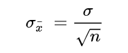
Where:

σ – Population standard deviation
n – Sample size, i.e., the number of observations in the sample

In a situation where statisticians are ignorant of the population standard deviation, they use the sample standard deviation as the closest replacement. SEM can then be calculated using the following formula. One of the primary assumptions here is that observations in the sample are statistically independent.

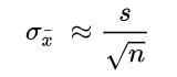
Where:

s – Sample standard deviation
n – Sample size, i.e., the number of observations in the sample

Importance of Standard Error

When a sample of observations is extracted from a population and the sample mean is calculated, it serves as an estimate of the population mean. Almost certainly, the sample mean will vary from the actual population mean. It will aid the statistician’s research to identify the extent of the variation. It is where the standard error of the mean comes into play.

When several random samples are extracted from a population, the standard error of the mean is essentially the standard deviation of different sample means from the population mean.

However, multiple samples may not always be available to the statistician. Fortunately, the standard error of the mean can be calculated from a single sample itself. It is calculated by dividing the standard deviation of the observations in the sample by the square root of the sample size.

Relationship between SEM and the Sample Size

Intuitively, as the sample size increases, the sample becomes more representative of the population.

For example, consider the marks of 50 students in a class in a mathematics test. Two samples A and B of 10 and 40 observations, respectively, are extracted from the population. It is logical to assert that the average marks in sample B will be closer to the average marks of the whole class than the average marks in sample A.

Thus, the standard error of the mean in sample B will be smaller than that in sample A. The standard error of the mean will approach zero with the increasing number of observations in the sample, as the sample becomes more and more representative of the population, and the sample mean approaches the actual population mean.

It is evident from the mathematical formula of the standard error of the mean that it is inversely proportional to the sample size. It can be verified using the SEM formula that if the sample size increases from 10 to 40 (becomes four times), the standard error will be half as big (reduces by a factor of 2).

Standard Deviation vs. Standard Error of the Mean

Standard deviation and standard error of the mean are both statistical measures of variability. While the standard deviation of a sample depicts the spread of observations within the given sample regardless of the population mean, the standard error of the mean measures the degree of dispersion of sample means around the population mean.

How accurate is our estimate of the mean?

Let’s revisit the first few days during which we collected data stored in the vector heights_island1. We were able to verify that the heights were normally distributed and calculated our sample mean, ({bar{x}}). However, we know that ({bar{x}}) is only an estimate of the true population mean, ({mu}), which is the true value of interest. It is unlikely that we will ever know the value of ({mu}), since access to all possible observations is rare. Therefore we will have to rely on ({bar{x}}) estimates from random samples drawn from the population as the best approximation of ({mu}).

Not all sample means are created equal. Some are better estimates than others. Recall the animation showing the relationship between sample size and variability of the mean. As we learned from this animation, in the long-run, large samples are necessary to get an accurate estimate of ({mu}).

A note about language: here, words like “accuracy”, “precision”, and “uncertainty” are used in a rather fast and loose way. We’re using the laymen’s application of these terms to refer to the long-run variability of estimates produced from repeated, independent trials. There are stricter, more formal statistical uses for these words, but for right now, we’re going to ignore these nuances so that we can move on with understanding these concepts in broad strokes.

One reason we care about our sample estimate’s accuracy is because we want to be able to answer questions about the population by making inferences. Statistical inference uses math to draw conclusions about the population based on a subset of the full picture (i.e. a sample). Subsets of data are of course limited, so it’s therefore important to acknowledge that the strength of the conclusions drawn about the population is dependent on the precision of the sample estimate. For example, say that we guess that the population mean value of giraffe heights on Island 1 is less than 11 cm. We can make some inferences about whether or not this is a good guess based on what we learn from our sample of giraffe heights. We’ll revisit this question a few times below.

Creating a sampling distribution

The mean of our sample of 50 giraffes from Island 1 was:

mean(heights_island1)

## [1] 9.714141

How can we quantify the accuracy of this estimate, given its sample size?

In theory, one way to illustrate this is to generate data not just from a single sample but from many samples of the same size (N) drawn from the same population.

Imagine that after you collected all 50 measurements for heights_island1, you wake up one morning with no memory of collecting data at all—and so you go out and collect 50 giraffe heights again and subsequently calculate the mean. Further imagine that this groundhog day (or more correctly, groundhog week) situation repeats itself many, many times.

When you finally return to your sanity, you find stacks of notebooks filled with mean values from each of your individual data collections.

Instead of viewing this as a massive waste of time, you make the best out of the situation and create a histogram of all the means. In other words you create a plot showing the distribution of the sample means, also known as a sampling distribution.

The animation below illustrates the process of creating the sampling distribution for 1,000 sample means.

On the left side, each histogram represents a sample (e.g. heights_island1 would be one sample, and we’re flashing through 1,000 of them in total). Correspondingly, each dot signifies an observation. After each sample histogram is completed, ({bar{x}}) is calculated. This ({bar{x}}) value is then subsequently added to the histogram of the sampling distribution on the right. As you can see below, this process is repeated, allowing the sampling distribution to build up.

A histogram of the sampling distribution is shown below. It is a histogram made up of many means.

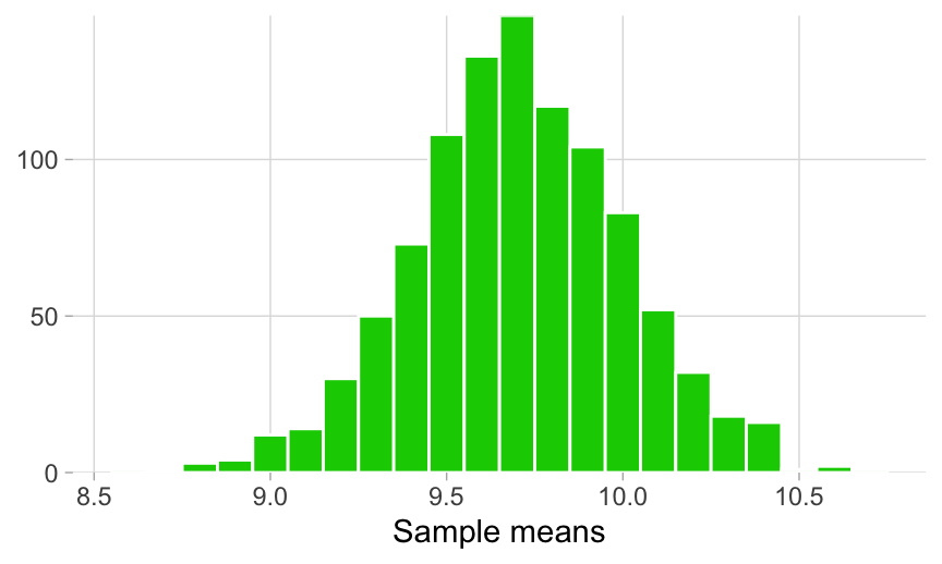
Looking at the spread of ({bar{x}}) values that this groundhog experience generated, we can get a sense of the range of many possible estimates of ({mu}) that a sample of 50 giraffes can produce.

The sampling distribution provides us with the first hint of the precision of our original heights_island1 estimate, which we’ll quantify in more detail later on, but for now it’s enough to notice that the range of possible ({bar{x}}) values are between 8.9 and 10.7. This means that ({bar{x}}) values outside of this range are essentially improbable.

Let’s return to our question about whether the true mean of giraffe heights on Island 1 is less than 11 cm. Our sampling distribution suggests that ({mu}) is less than 11 cm, since values greater than that are not within the range of this sampling distribution.

Sample size and sampling distribution

Back to the idea that larger samples are “better”, we can explore what happens if we redo the groundhog scenario, this time sampling 500 individuals (instead of 50) before taking the mean each time, repeating this until thousands of ({bar{x}}) values have been recorded. For completeness, let’s imagine the same marathon data collection using samples that are smaller—of 5 giraffes each. We compare the resulting sampling distributions from all three scenarios below. The middle sampling distribution corresponds to the sampling distribution we already generated above.

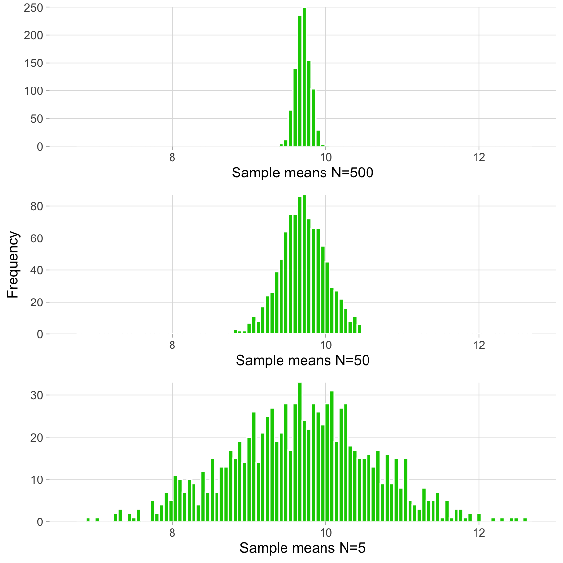
What do we notice?

All histograms look normal.
All distributions have approximately the same mean.
Distributions generated from larger samples are less dispersed.

We can take the mean of the sampling distribution itself– the mean of the sampling distribution is a mean of means. This mean can be interpreted to be the same as a mean that would have resulted from a single large sample, made up of all the individual observations from each of the samples whose ({bar{x}}) values are included in the sampling distribution.

Note that if we had only generated a sampling distribution made up of samples of 5 giraffes, we would not have been able to exclude 11 cm as a possible value for ({mu}). In fact, if we were to draw a vertical line in the middle of each of the sampling distributions (the mean), we can tell that the population mean is likely even less than 10 cm.

In the following window, you will test the relationship between sampling distribution and sample size. The function below (behind-the-scenes code not shown) will plot a sampling distribution made up of 1000 samples, with each sample containing N number of observations. Try setting N to a few different values. What does the resulting sampling distribution looks like? See if you can confirm for yourself that the above points are true.

Standard Error of the Mean

As we’ve done before, we want to summarize this spread of mean estimates with a single value. We’ve already learned how to quantify a measure of spread–the standard deviation. If we take the standard deviations of each of the three different sampling scenarios above, then we accept that distributions based on smaller samples should have larger standard deviations.

In the window below, calculate the standard deviation of each of the three sampling distributions (i.e. for N = 500, N = 50, and N = 5), and confirm that the italicized point above is true. (If you’re working in R locally, use your “homemade” standard deviation function from the Variance module.)

To complete this exercise, you will need to use the objects sampling_distribution_N500, sampling_distribution_N50, sampling_distribution_N5, which are vectors storing the thousands of ({bar{x}}) values from the corresponding groundhog sampling distributions.

When you calculate the standard deviation of a sampling distribution of ({bar{x}}) values, you are calculating the standard error of the mean (SEM), or just “standard error”. The SEM is the value that we use to capture the level of precision of our sample estimate. But, we need a better and more efficient way to arrive at this value without relying on a groundhog day situation. Keep reading to learn more.

A note about SEM: Here “standard error” will imply standard error of the mean. But we can technically calculate the standard error of any sample statistic, not just the mean. We’ll talk about that more in future modules.

Time for a tea break!

Standard error in practice

Deriving the equation used for calculating the standard error of the mean using theory (i.e. without going out and resampling MANY times) is a bit complicated, but if you’re interested, you can learn more about it here. Instead, we can capture the relationship between standard deviation, sample size, and standard error with the plot below.

The standard deviation in this plot is 2.1, which represents ({sigma}) for giraffe heights on Island 1. This population value is technically still unknown but can be deduced in theory by repeating the groundhog day example for the standard deviation instead of for the mean. It’s important to note that the plot would have the same shape regardless of what scenario or standard deviation we were using.

Can you figure out what the equation is for the SEM? Look at the plot above, hover over the points, and see if you can gather how standard error of the mean, standard deviation, and sample size are related. Here are some hints:

SEM will be on one side of the equation, standard devation, and N will be on the other.
The equation will involve division.
There is one more missing piece of the puzzle: When you look at the shape of the plot above. What type of function does this remind you of? We haven’t covered this explicitly, but take a look here and see if you get any ideas.

Use the window below as a calculator to see if you can figure out the equation for the SEM.

In case you weren’t able to figure it out, remember to check the Solutions tab in the exercise window or take a look at this link for the equation for calculating the SEM. Recall that we’re working with the sample (and not population) standard deviation ((s)), so make sure you find the correct equation.

Confirming that the SEM equation works

Let’s test out the SEM equation on our original sample of heights_island1 and compare it to what we would have gotten by taking the standard deviation of the sampling distribution example with the N= 50 case. Does the SEM seem like a good approximation of the standard deviation of the sampling distribution?

Below, you will use the object heights_island1, which contains our single sample of N=50, and the object sampling_distribution_N50, which contains the data from the corresponding groundhog sampling distribution.

Close enough! We wouldn’t expect these to be exactly the same because of sampling variability.

How do we apply the SEM?

Now that we have a better understanding of how to gauge the precision of our sample estimates, we can test our question about the ({mu}) being less than 11 cm once and for all.

To formally make inferences, we need to revisit the principles of the empirical rule to construct confidence intervals. (Confidence intervals are just one way to make inferences– we’ll discuss other ways later.)

Remember, that the SEM is just the standard deviation of the sampling distribution, so we can apply the empirical rule. As a result, ± 2 SEM from a point estimate will capture ~95% of the sampling distribution. Actually, we were a little bit sloppy earlier when we said 2 standard deviations captures 95% of a normal distribution; this will actually give you 95.45% of the data. The true value is 1.96 standard deviations–and this is what we use to construct a 95% confidence interval (CI).

Loosely speaking, a 95% CI is the range of values that we are 95% confident contains the true mean of the population. We want to know whether our guess of 11 cm falls outside of this range of certainty. If it does – we can be sure enough that the true ({mu}) of giraffe heights on Island 1 is less than 11 cm.

Use the window below to find out and make your first inference by constructing the 95% CI for the heights_island1 mean estimate!

The upper limit of our 95% CI is less than 11 cm, so the population mean of heights on island 1 is likely less than 11 cm. In the scientific community, this is a bonafide way of drawing this conclusion.

Things to think about

We’ve been a little fast and loose with our words. The formal definition of CIs is the following:

If we were to sample over and over again, then 95% of the time the CIs would contain the true mean.

Importantly, some examples of what the 95% CI does NOT mean are:

A 95% CI does not mean that it contains 95% of the sample data.
A CI is not a definitive range of likely values for the sample statistic, but you can think of it as estimate of likely values for the population parameter.
It does not mean that values outside of the 95% CI have a 5% chance of being the true mean.

The precise interpretation of CIs is quite a nuanced and rather hotly debated topic see here and becomes somewhat philosophical– so if these definition subtleties seem confusing, don’t feel bad. As mentioned in the blog post linked above, one recent paper reported that 97% of surveyed researchers endorsed at least one misconception (out of 6) about CIs.

Источник

A standard error of measurement, often denoted SE_m, estimates the variation around a “true” score for an individual when repeated measures are taken.

It is calculated as:

SE_m = s√1-R

where:

s: The standard deviation of measurements
R: The reliability coefficient of a test

Note that a reliability coefficient ranges from 0 to 1 and is calculated by administering a test to many individuals twice and calculating the correlation between their test scores.

The higher the reliability coefficient, the more often a test produces consistent scores.

Example: Calculating a Standard Error of Measurement

Suppose an individual takes a certain test 10 times over the course of a week that aims to measure overall intelligence on a scale of 0 to 100. They receive the following scores:

Scores: 88, 90, 91, 94, 86, 88, 84, 90, 90, 94

The sample mean is 89.5 and the sample standard deviation is 3.17.

If the test is known to have a reliability coefficient of 0.88, then we would calculate the standard error of measurement as:

SE_m = s√1-R = 3.17√1-.88 = 1.098

How to Use SE_m to Create Confidence Intervals

Using the standard error of measurement, we can create a confidence interval that is likely to contain the “true” score of an individual on a certain test with a certain degree of confidence.

If an individual receives a score of x on a test, we can use the following formulas to calculate various confidence intervals for this score:

68% Confidence Interval = [x – SE_m, x + SE_m]
95% Confidence Interval = [x – 2*SE_m, x + 2*SE_m]
99% Confidence Interval = [x – 3*SE_m, x + 3*SE_m]

For example, suppose an individual scores a 92 on a certain test that is known to have a SE_m of 2.5. We could calculate a 95% confidence interval as:

95% Confidence Interval = [92 – 2*2.5, 92 + 2*2.5] = [87, 97]

This means we are 95% confident that an individual’s “true” score on this test is between 87 and 97.

Reliability & Standard Error of Measurement

There exists a simple relationship between the reliability coefficient of a test and the standard error of measurement:

The higher the reliability coefficient, the lower the standard error of measurement.
The lower the reliability coefficient, the higher the standard error of measurement.

To illustrate this, consider an individual who takes a test 10 times and has a standard deviation of scores of 2.

If the test has a reliability coefficient of 0.9, then the standard error of measurement would be calculated as:

SE_m = s√1-R = 2√1-.9 = 0.632

However, if the test has a reliability coefficient of 0.5, then the standard error of measurement would be calculated as:

SE_m = s√1-R = 2√1-.5 = 1.414

This should make sense intuitively: If the scores of a test are less reliable, then the error in the measurement of the “true” score will be higher.

Источник

Standard error of the sample mean[edit]

Exact value[edit]

Estimate[edit]

Accuracy of the estimator[edit]

Derivation[edit]

Independent and identically distributed random variables with random sample size[edit]

Student approximation when σ value is unknown[edit]

Assumptions and usage[edit]

Standard error of mean versus standard deviation[edit]

Extensions[edit]

Finite population correction (FPC)[edit]

Correction for correlation in the sample[edit]

See also[edit]

References[edit]

Standard Error of the Mean vs. Standard Deviation: An Overview

Key Takeaways

Click Play to Learn the Difference Between Standard Error and Standard Deviation

Calculating SD and SEM

Standard Deviation

Standard Error of the Mean

Standard Error and Standard Deviation in Finance

How Are Standard Deviation and Standard Error of the Mean Different?

Is the Standard Error Equal to the Standard Deviation?

How Can You Compute the SE From the SD?

Why Do We Use Standard Error Instead of Standard Deviation?

What Is the Empirical Rule, and How Does It Relate to Standard Deviation?

The Bottom Line

Способ 1: используйте SciPy

Способ 2: использовать NumPy

Как интерпретировать стандартную ошибку среднего

Дополнительные ресурсы

What is Standard Error?

Calculating Standard Error of the Mean (SEM)

<img decoding="async" onError="javascript: wp_broken_images = window.wp_broken_images || function(){}; wp_broken_images(this);" loading="lazy" src="https://cdn.corporatefinanceinstitute.com/assets/standard-error1.png" alt="Standard Error - Formula" width="200" height="83" />

Importance of Standard Error

Relationship between SEM and the Sample Size

Standard Deviation vs. Standard Error of the Mean

Related Readings

How accurate is our estimate of the mean?

Creating a sampling distribution

Sample size and sampling distribution

Standard Error of the Mean

Time for a tea break!

Standard error in practice

Confirming that the SEM equation works

How do we apply the SEM?

Things to think about

Example: Calculating a Standard Error of Measurement

How to Use SEm to Create Confidence Intervals

Reliability & Standard Error of Measurement

How to Use SE_m to Create Confidence Intervals