From Wikipedia, the free encyclopedia

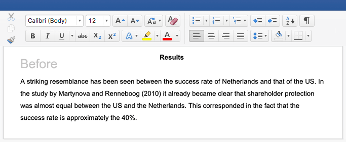
For a value that is sampled with an unbiased normally distributed error, the above depicts the proportion of samples that would fall between 0, 1, 2, and 3 standard deviations above and below the actual value.
The standard error (SE)[1] of a statistic (usually an estimate of a parameter) is the standard deviation of its sampling distribution[2] or an estimate of that standard deviation. If the statistic is the sample mean, it is called the standard error of the mean (SEM).[1]
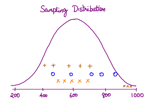
The sampling distribution of a mean is generated by repeated sampling from the same population and recording of the sample means obtained. This forms a distribution of different means, and this distribution has its own mean and variance. Mathematically, the variance of the sampling mean distribution obtained is equal to the variance of the population divided by the sample size. This is because as the sample size increases, sample means cluster more closely around the population mean.
Therefore, the relationship between the standard error of the mean and the standard deviation is such that, for a given sample size, the standard error of the mean equals the standard deviation divided by the square root of the sample size.[1] In other words, the standard error of the mean is a measure of the dispersion of sample means around the population mean.
In regression analysis, the term «standard error» refers either to the square root of the reduced chi-squared statistic or the standard error for a particular regression coefficient (as used in, say, confidence intervals).
Standard error of the sample mean[edit]
Exact value[edit]
Suppose a statistically independent sample of  observations
  is taken from a statistical population with a standard deviation of
  . The mean value calculated from the sample,
  , will have an associated standard error on the mean,
  , given by:[1]
 .
.

Practically this tells us that when trying to estimate the value of a population mean, due to the factor  , reducing the error on the estimate by a factor of two requires acquiring four times as many observations in the sample; reducing it by a factor of ten requires a hundred times as many observations.
Estimate[edit]
The standard deviation of the population being sampled is seldom known. Therefore, the standard error of the mean is usually estimated by replacing with the sample standard deviation  instead:
- .

As this is only an estimator for the true «standard error», it is common to see other notations here such as:
- or alternately .


A common source of confusion occurs when failing to distinguish clearly between:
Accuracy of the estimator[edit]
When the sample size is small, using the standard deviation of the sample instead of the true standard deviation of the population will tend to systematically underestimate the population standard deviation, and therefore also the standard error. With n = 2, the underestimate is about 25%, but for n = 6, the underestimate is only 5%. Gurland and Tripathi (1971) provide a correction and equation for this effect.[3] Sokal and Rohlf (1981) give an equation of the correction factor for small samples of n < 20.[4] See unbiased estimation of standard deviation for further discussion.
Derivation[edit]
The standard error on the mean may be derived from the variance of a sum of independent random variables,[5] given the definition of variance and some simple properties thereof. If are independent samples from a population with mean and standard deviation , then we can define the total

which due to the Bienaymé formula, will have variance

where we’ve approximated the standard deviations, i.e., the uncertainties, of the measurements themselves with the best value for the standard deviation of the population. The mean of these measurements is simply given by
- .

The variance of the mean is then

The standard error is, by definition, the standard deviation of which is simply the square root of the variance:
- .

For correlated random variables the sample variance needs to be computed according to the Markov chain central limit theorem.
Independent and identically distributed random variables with random sample size[edit]
There are cases when a sample is taken without knowing, in advance, how many observations will be acceptable according to some criterion. In such cases, the sample size  is a random variable whose variation adds to the variation of
  such that,
- [6]

If has a Poisson distribution, then  with estimator
  . Hence the estimator of
  becomes
  , leading the following formula for standard error:

(since the standard deviation is the square root of the variance)
Student approximation when σ value is unknown[edit]
In many practical applications, the true value of σ is unknown. As a result, we need to use a distribution that takes into account that spread of possible σ’s.
When the true underlying distribution is known to be Gaussian, although with unknown σ, then the resulting estimated distribution follows the Student t-distribution. The standard error is the standard deviation of the Student t-distribution. T-distributions are slightly different from Gaussian, and vary depending on the size of the sample. Small samples are somewhat more likely to underestimate the population standard deviation and have a mean that differs from the true population mean, and the Student t-distribution accounts for the probability of these events with somewhat heavier tails compared to a Gaussian. To estimate the standard error of a Student t-distribution it is sufficient to use the sample standard deviation «s» instead of σ, and we could use this value to calculate confidence intervals.
Note: The Student’s probability distribution is approximated well by the Gaussian distribution when the sample size is over 100. For such samples one can use the latter distribution, which is much simpler.
Assumptions and usage[edit]
An example of how  is used is to make confidence intervals of the unknown population mean. If the sampling distribution is normally distributed, the sample mean, the standard error, and the quantiles of the normal distribution can be used to calculate confidence intervals for the true population mean. The following expressions can be used to calculate the upper and lower 95% confidence limits, where is equal to the sample mean, is equal to the standard error for the sample mean, and 1.96 is the approximate value of the 97.5 percentile point of the normal distribution:
- Upper 95% limit and
- Lower 95% limit


In particular, the standard error of a sample statistic (such as sample mean) is the actual or estimated standard deviation of the sample mean in the process by which it was generated. In other words, it is the actual or estimated standard deviation of the sampling distribution of the sample statistic. The notation for standard error can be any one of SE, SEM (for standard error of measurement or mean), or SE.
Standard errors provide simple measures of uncertainty in a value and are often used because:
- in many cases, if the standard error of several individual quantities is known then the standard error of some function of the quantities can be easily calculated;
- when the probability distribution of the value is known, it can be used to calculate an exact confidence interval;
- when the probability distribution is unknown, Chebyshev’s or the Vysochanskiï–Petunin inequalities can be used to calculate a conservative confidence interval; and
- as the sample size tends to infinity the central limit theorem guarantees that the sampling distribution of the mean is asymptotically normal.
Standard error of mean versus standard deviation[edit]
In scientific and technical literature, experimental data are often summarized either using the mean and standard deviation of the sample data or the mean with the standard error. This often leads to confusion about their interchangeability. However, the mean and standard deviation are descriptive statistics, whereas the standard error of the mean is descriptive of the random sampling process. The standard deviation of the sample data is a description of the variation in measurements, while the standard error of the mean is a probabilistic statement about how the sample size will provide a better bound on estimates of the population mean, in light of the central limit theorem.[7]
Put simply, the standard error of the sample mean is an estimate of how far the sample mean is likely to be from the population mean, whereas the standard deviation of the sample is the degree to which individuals within the sample differ from the sample mean.[8] If the population standard deviation is finite, the standard error of the mean of the sample will tend to zero with increasing sample size, because the estimate of the population mean will improve, while the standard deviation of the sample will tend to approximate the population standard deviation as the sample size increases.
Extensions[edit]
Finite population correction (FPC)[edit]
The formula given above for the standard error assumes that the population is infinite. Nonetheless, it is often used for finite populations when people are interested in measuring the process that created the existing finite population (this is called an analytic study). Though the above formula is not exactly correct when the population is finite, the difference between the finite- and infinite-population versions will be small when sampling fraction is small (e.g. a small proportion of a finite population is studied). In this case people often do not correct for the finite population, essentially treating it as an «approximately infinite» population.
If one is interested in measuring an existing finite population that will not change over time, then it is necessary to adjust for the population size (called an enumerative study). When the sampling fraction (often termed f) is large (approximately at 5% or more) in an enumerative study, the estimate of the standard error must be corrected by multiplying by a »finite population correction» (a.k.a.: FPC):[9]
[10]

which, for large N:

to account for the added precision gained by sampling close to a larger percentage of the population. The effect of the FPC is that the error becomes zero when the sample size n is equal to the population size N.
This happens in survey methodology when sampling without replacement. If sampling with replacement, then FPC does not come into play.
Correction for correlation in the sample[edit]

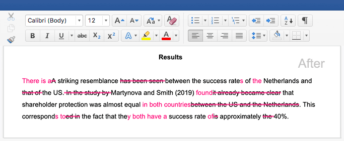
Expected error in the mean of A for a sample of n data points with sample bias coefficient ρ. The unbiased standard error plots as the ρ = 0 diagonal line with log-log slope −½.
If values of the measured quantity A are not statistically independent but have been obtained from known locations in parameter space x, an unbiased estimate of the true standard error of the mean (actually a correction on the standard deviation part) may be obtained by multiplying the calculated standard error of the sample by the factor f:

where the sample bias coefficient ρ is the widely used Prais–Winsten estimate of the autocorrelation-coefficient (a quantity between −1 and +1) for all sample point pairs. This approximate formula is for moderate to large sample sizes; the reference gives the exact formulas for any sample size, and can be applied to heavily autocorrelated time series like Wall Street stock quotes. Moreover, this formula works for positive and negative ρ alike.[11] See also unbiased estimation of standard deviation for more discussion.
See also[edit]
- Illustration of the central limit theorem
- Margin of error
- Probable error
- Standard error of the weighted mean
- Sample mean and sample covariance
- Standard error of the median
- Variance
References[edit]
- ^ a b c d Altman, Douglas G; Bland, J Martin (2005-10-15). «Standard deviations and standard errors». BMJ: British Medical Journal. 331 (7521): 903. doi:10.1136/bmj.331.7521.903. ISSN 0959-8138. PMC 1255808. PMID 16223828.
- ^ Everitt, B. S. (2003). The Cambridge Dictionary of Statistics. CUP. ISBN 978-0-521-81099-9.
- ^ Gurland, J; Tripathi RC (1971). «A simple approximation for unbiased estimation of the standard deviation». American Statistician. 25 (4): 30–32. doi:10.2307/2682923. JSTOR 2682923.
- ^ Sokal; Rohlf (1981). Biometry: Principles and Practice of Statistics in Biological Research (2nd ed.). p. 53. ISBN 978-0-7167-1254-1.
- ^ Hutchinson, T. P. (1993). Essentials of Statistical Methods, in 41 pages. Adelaide: Rumsby. ISBN 978-0-646-12621-0.
- ^ Cornell, J R, and Benjamin, C A, Probability, Statistics, and Decisions for Civil Engineers, McGraw-Hill, NY, 1970, ISBN 0486796094, pp. 178–9.
- ^ Barde, M. (2012). «What to use to express the variability of data: Standard deviation or standard error of mean?». Perspect. Clin. Res. 3 (3): 113–116. doi:10.4103/2229-3485.100662. PMC 3487226. PMID 23125963.
- ^ Wassertheil-Smoller, Sylvia (1995). Biostatistics and Epidemiology : A Primer for Health Professionals (Second ed.). New York: Springer. pp. 40–43. ISBN 0-387-94388-9.
- ^ Isserlis, L. (1918). «On the value of a mean as calculated from a sample». Journal of the Royal Statistical Society. 81 (1): 75–81. doi:10.2307/2340569. JSTOR 2340569. (Equation 1)
- ^ Bondy, Warren; Zlot, William (1976). «The Standard Error of the Mean and the Difference Between Means for Finite Populations». The American Statistician. 30 (2): 96–97. doi:10.1080/00031305.1976.10479149. JSTOR 2683803. (Equation 2)
- ^ Bence, James R. (1995). «Analysis of Short Time Series: Correcting for Autocorrelation». Ecology. 76 (2): 628–639. doi:10.2307/1941218. JSTOR 1941218.
The standard error (SE) of the sample mean refers to the standard deviation of the distribution of the sample means. It gives analysts an estimate of the variability they would expect if they were to draw multiple samples from the same population. While the standard deviation measures the variability obtained within one sample, the standard error gives an estimate of the variability between many samples.
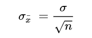
Provided the population standard deviation, σ, is known, analysts use the following formula to estimate the standard error of the sample mean, denoted as σx:
$$ sigma_x=cfrac {sigma}{sqrt n} $$
Where n is the sample size.
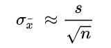
However, the population standard deviation, σ, is usually unknown. In such a case, the following formula is used to estimate the standard error of the sample mean, also denoted as Sx:
$$ S_x =cfrac {S}{sqrt n} $$
Where S is the sample standard deviation; and (S^2 =cfrac {sum left(X_i- X right)^2}{n- 1} ).
Breaking Down the Standard Error of the Sample Mean
The standard error of the sample mean gives analysts an idea of how precisely the sample mean estimates the population mean. A lower value of the standard error indicates a more precise estimation of the population mean. On the other hand, a larger value of the standard error indicates a less precise estimate of the population mean.
It’s also important to note that the standard error becomes smaller as the sample size increases. This happens because increasing the sample size ultimately brings the sample mean closer to the true value of the population mean.
Example: Calculating the Standard Error of the Sample Mean When the Population Standard Deviation is Known
In a certain property investment company with an international presence, workers have a mean hourly wage of $12 with a population standard deviation of $3. Given a sample size of 30, estimate and interpret the SE of the sample mean:
$$ begin{align*} sigma_x & =cfrac {sigma}{sqrt n} \ & =cfrac {3}{sqrt {30}} \ & = $0.55 \ end{align*} $$
Interpretation: if we were to draw several samples of size 30 from the employee population and construct a sampling distribution of the sample means, we would end up with a mean of $12 and a standard error of $0.55.
Example: Calculating the Standard Error of the Sample Mean When σ is Unknown
A sample of 30 latest returns on XYZ stock reveals a mean return of $4 with a sample standard deviation of $0.13. Estimate the SE of the sample mean.
$$ begin{align*} S_x & =cfrac {S}{sqrt n} \ & =cfrac {0.13}{sqrt {30}} \ & = $0.02 \ end{align*} $$
Interpretation: If we were to draw more samples from the population of yearly returns on XYZ stock and construct a sample mean distribution, we would end up with a mean of $4 and a standard error of $0.02.
Question
Assume that we have increased the sample size to 80 in the example above and derived similar values for the mean and standard deviation of returns. Estimate the standard error of the sample mean.
A. 0.01
B. 0.02
C. 0.08
Solution
The correct answer is A.
$$ begin{align*} S_x & =cfrac {S}{sqrt n} \ & = cfrac {0.13}{sqrt {80}} \ & = $0.01 \ end{align*} $$
This clearly proves that increasing the sample size reduces the SE of the sample mean.
Reading 10 LOS 10f:
Calculate and interpret the standard error of the sample mean
Standard error of the mean measures how spread out the means of the sample can be from the actual population mean. Standard error allows you to build a relationship between a sample statistic (computed from a smaller sample of the population) and the population’s actual parameter.
 Standard Error – A practical guide with examples. Photo by Sergio.
What is Standard Error?
The sample error serves as a means to understand the actual population parameter (like population mean) without actually estimating it.
Consider the following scenario:
A researcher ‘X’ is collecting data from a large population of voters. For practical reasons he can’t reach out to each and every voter. So, only a small randomized sample (of voters) is selected for data collection.
Once the data for the sample is collected, you calculate the mean (or any statistic) of that sample. But then, this mean you just computed is only the sample mean. It cannot be considered the entire population’s mean. You can however expect it to be somewhere close to population’s mean.
So how can you know the actual population mean?
While its not possible to compute the exactly value, you can use standard error to estimate how far the sample mean may spread from the actual population mean.
To be more precise,
The Standard Error of the Mean describes how far a sample mean may vary from the population mean.
In this post, you will understand clearly:
- What Standard Error Tells Us?
- What is the Sample Error Formula?
- How to calculate Standard Error?
- How to use standard error to compute confidence interval?
- Example Problem and solution
How to understand Standard Error?
Let’s first clearly understand the intuition behind and the need for standard error.
Now, let’s suppose you are working in agriculture domain and you want to know the annual yield of a particular variety of coconut trees. While the entire population of coconut trees has a certain mean (and standard deviation) of annual yield, it is not practical to take measurements of each and every tree out there.
So, what do you do?
To estimate this you collect samples of coconut yield (number of nuts per tree per year) from different trees. And to keep your findings unbiased, you collect samples across different places.
MLPlus Industry Data Scientist Program
Do you want to learn Data Science from experienced Data Scientists?
Build your data science career with a globally recognised, industry-approved qualification. Solve projects with real company data and become a certified Data Scientist in less than 12 months.
.
![]()
Get Free Complete Python Course
Build your data science career with a globally recognised, industry-approved qualification. Get the mindset, the confidence and the skills that make Data Scientist so valuable.
Let’s say, you collected data from approx ~5 trees per sample from different places and the numbers are shown below.
# Annual yield of coconut
sample1 = [400, 420, 470, 510, 590]

sample2 = [430, 500, 570, 620, 710, 800, 900]

sample3 = [360, 410, 490, 550, 640]
In above data, the variables sample1, sample2 and sample3 contain the samples of annual yield values collected, where each number represents the yield of one individual tree.
Observe that the yield varies not just across the trees, but also across the different samples.
Although we compute means of the samples, we are actually not interested in the means of the sample, but the overall mean annual yield of coconut of this variety.
Now, you may ask: ‘Why can’t we just put the values from all these samples in one bucket and simply compute the mean and standard deviation and consider that as the population’s parameter?‘
Well, the problem is, if you do that practically what happens is, as you receive few more samples, the real population’s parameter begins to come out which is likely to be (slightly) different from the parameter you computed earlier.
Below is a code demo.
from statistics import mean, stdev

# Overall mean from the first two samples
sample1 = [400, 420, 470, 510, 590]
sample2 = [430, 500, 570, 620, 710, 800, 900]
print("Mean of first two samples: ", mean(sample1 + sample2))

# Overall mean after introducing 3rd sample
sample3 = [360, 410, 490, 550, 640]
print("Mean after including 3rd sample: ", mean(sample1 + sample2 + sample3))
Output:
Mean of first two samples:  576.6666666666666
Mean after including 3rd sample:  551.1764705882352
As you add more and more samples, the computed parameters keep changing.
So how to tackle this?
If you notice, each sample has its own mean that varies between a particular range. This mean (of the sample) has its own standard deviation. This measure of standard deviation of the mean is called the standard error of the mean.
Its important to note, it is different from the standard deviation of the data. The difference is, while standard deviation tells you how the overall data is distributed around the mean, the standard error tells you how the mean itself is distributed.
This way, it can be used to generalize the sample mean so it can be used as an estimate of the whole population.
In fact, standard error can be generalized to any statistic like standard deviation, median etc. For example, if you compute the standard deviation of the standard deviations (of the samples), it is called, standard error of the standard deviation. Feels like a tongue twister. But most commonly, when someone mention ‘Standard error’ it typically refers to the ‘Standard error of of the mean’.
What is the Formula?
To calculate standard error, you simply divide the standard deviation of a given sample by the square root of the total number of items in the sample.
$$SE_{bar{x}} = frac{sigma}{sqrt{n}}$$
where, $SE_{bar{x}}$ is the standard error of the mean, $sigma$ is the standard deviation of the sample and n is the number of items in sample.
Do not confuse this with standard deviation. Because standard error of the sample statistic (like mean) is typically much smaller than the population standard deviation.
Notice few things here:
- The Standard error depends on the number of items in the sample. As you increase the number of items in the sample, lower will be the standard error and more certain you will be about the estimates.
- It uses statistics (standard deviation and number of items) computed from the sample itself, and not of the population. That is, you don’t need to know the population parameters beforehand to compute standard error. This makes it pretty convenient.
- Standard error can also be used as an estimate of how representative a given sample is of a population. The smaller the value, more representative is the sample of the whole population.
Below is a computation for the standard error of the mean:
# Compute Standard Error
sample1 = [400, 420, 470, 510, 590]
se = stdev(sample1)/len(sample1)
print('Standard Error: ', round(se, 2))
Standard Error: 15.19
How to calculate standard error?
Problem Statement
A school aptitude test for 15 year old students studying in a particular territory’s curriculum, is designed to have a mean score of 80 units and a standard deviation of 10 units. A sample of 15 answer papers has a mean score of 85. Can we assume that these 15 scores come from the designated population?
Solution
Our task is to determine if this sample comes from the above mentioned population.
How to solve this?
We approach this problem by computing the standard error of the sample means and use it to compute the confidence interval between which the sample means are expected to fall.
If the given sample mean falls inside this interval, then its safe to assume that the sample comes from the given population.
Time to get into the math.
Using standard error to compute confidence interval
Standard error is often used to compute confidence intervals
We know, n = 15, x_bar = 85, σ = 10
$$SE_bar{x} = frac{sigma}{sqrt{n}} = frac{10}{sqrt{15}} = 2.581$$
From a property of normal distribution, we can say with 95% confidence level that the sample means are expected to lie within a confidence interval of plus or minus two standard errors of the sample statistic from the population parameter.
But where did ‘normal distribution’ come from? You may wonder how we can directly assume a normal distribution is followed in this case. Or rather shouldn’t we test if the sample follows a normal distribution first before computing the confidence intervals.
Well, that’s NOT required. Because, the Central Limit Theorem tells us that even if a population is not normally distributed, a collection of sample means from that population will infact follow a normal distribution. So, its a valid assumption.
Back to the problem, let’s compute the confidence intervals for 95% Confidence Level.
- Lower Limit :
80 - (2*2.581)= 74.838 - Upper Limit :
80 + (2*2.581)= 85.162
So, 95% of our 15 item sample means are expected to fall between 74.838 and 85.162.
Since the sample mean of 85.0 lies within the computed range, there is no reason to believe that the sample does not belong to the population.
Conclusion
Standard error is a commonly used term that we sometimes ignore to fully understand its significance. I hope the concept is clear and you can now relate how you can use standard error in appropriate situations.
Next topic: Confidence Interval
Want to join the conversation?
-
Why is it called standard error of the mean even though it is the standard deviation of the sampling distribution of the sample mean?
Button navigates to signup pageButton navigates to signup page
-
It is called an error because the standard deviation of the sampling distribution tells us how different a sample mean can be expected to be from the true mean. In other words, if we assume that the mean of our sample is always the true mean (even though it probably isn’t) the standard deviation can tell us how likely we are to be wrong.
Button navigates to signup page
-
-
Isn’t CLT not just an extension of law of large numbers?
Button navigates to signup pageButton navigates to signup page
-
This is correct but I think students can potentially misunderstand this concept.
A good way to think of the data sets that one uses for Standard Error and CLT is that the data sets we are using contain mean values of a population.
Button navigates to signup page
-
-
Can you help me understand when we use (sigma)/(√n) rather than just using sigma? For example, when we are calculating z-scores, I am so confused as to when we say (x-bar — mu) / ((sigma)/(√n)) rather than (x-bar — mu) / (sigma). Can anyone help?
Button navigates to signup pageButton navigates to signup page
-
The proof is based on this basic property of random variables:
For three random variables X, Y and Z,
(1) if Z=mX + mY = m(X + Y),
(2) then Var[Z] = m^2*Var[X] + m^2*Var[Y] = m^2(Var[X] + Var[Y]).Similarly, by taking a sample of size n and calculating its mean, we are creating a new random variable x-bar that is the sum of many random variables. Think of x-bar as Z, 1/n as m, and each sample point x(i) as X, Y, etc.:
(1) x-bar = (x(1) + x(2) + … + x(n))/n = 1/n * (x(1) + x(2) + … + x(n))
What is the variance of this new random variable x-bar? Apply the property from above:
(2) Var[x-bar] = 1/n^2 * (Var[x(1)] + Var[x(2)] + … + Var[x(n)])
When we take a sample of n data points, each individual point x(i) ‘inherits’ the population’s variance: Var[x(i)] = σ^2. This means we can simplify:
(2) Var[x-bar] = 1/n^2 * (σ^2 + σ^2 + … + σ^2) = n/n^2 * σ^2 = σ^2/n
This is just the variance for one sample. The sampling distribution is a combination of all these new random variables:
(1) Distribution = x-bar(1) + x-bar(2) + … + x-bar(n)
So the sampling distribution has variance:
(2) Var[Distribution] = 1/n^2 * (σ^2 + σ^2 + … + σ^2) = n/n^2 * σ^2 = σ^2/n
Finally, the sampling distribution’s standard error is the square root of the sampling distribution’s variance: σ/√n.
Comment on Jacob Kovacs’s post “The proof is based on thi…”
-
-
Why is the standard error of the mean so much more sensible to the number of things I am taking averages from than the number of times we take the average? This last number doesn’t even figure in the formula even though it did vary a bit in the experimental program (although seemingly not in a monotonic or convergent way!)
Button navigates to signup pageButton navigates to signup page
-
The process of averaging a certain number of samples from one distribution actually creates a NEW distribution. It’s that new distribution that you’re sampling from. So when Sal averages 16 samples, he’s creating one new distribution. When he averages 25 samples, he’s creating a different new distribution.
But from that point forward, taking a lot of averages is just sampling lots of times from that new distribution. So taking 10,000 samples from the average of 16 just gives you an idea of what that new distribution looks like.
If you had the mathematical equation for the original distribution, you can derive the equation for the new distribution. That equation will have a fixed mean and standard deviation, and taking more and more samples simply gives you more confidence in your estimate of the mean and standard deviation.
As far as the variation in the experimental program, think if it this way. It’s «possible» to take 100 samples that give you EXACTLY the mean and standard deviation of the new distribution. You just can’t know for certain that you actually got the right answer. If you take a billion samples, you have a lot more confidence that you’re really close, even if it isn’t exact. Over time, it will converge, but that convergence isn’t strict. It can fluctuate some while converging.
Comment on david.a.hooper’s post “The process of averaging …”
-
-
I read some book before that a normal distribution have a kurtosis of 3, how come the java have a kurtosis close to zero if it is approximately normal distributed?
Button navigates to signup pageButton navigates to signup page
-
I think the java application assumes 0 kurtosis for the normal curve. In other words, it subtracts 3 from the kurtosis achieved.
Button navigates to signup page
-
-
if the original data set only had 10000 data points, and i selected a sample size of n=10000, calculated x_bar 100 times, and created a frequency distribution, wouldn’t that just be a vertical bar? In that case the distribution doesn’t look very normal at all.
It would have no tails and no peaks, so how can the distribution look increasingly normal as n->∞ ? Are we assuming an arbitrarily large original data set? Wouldn’t it make more sense to say that the distribution looks increasingly normal with n as it initially increases, and then decreasingly normal with n as it approaches the size of the total original data set? Can we take partial derivatives and minimize for skew and kurtosis?
Also, if we can always get to an arbitrarily small variance by increasing n, aren’t we losing the meaning of the data? Isn’t it like blurring an image to the point where it’s all just one color? At some point the image is no longer recognizable.
Do we just keep iterating through variances until we’re happy? Is there a heuristic for preserving data integrity (in the non-image case where it’s not as easy to identify whether something is representative of the original data)?
Button navigates to signup pageButton navigates to signup page
-
If the population has N=10000, and the sample has n=10000, then there is no need to think about the sampling distribution. The sampling distribution is a way to describe how a statistic behaves from sample to sample, but if we sampled the whole population, then we can calculate the parameters directly.
More generally though, you seem to be getting at the idea of what happens as n->∞. Yes, it’s true that the standard error of the mean gets smaller and smaller as n increases, but it won’t get to the point of a distribution that’s just a single vertical bar (we’d call it a degenerate distribution). That’s too far out into n being large, it may be what «will eventually happen», but we can never actually get to that point.
And also, yes, we often assume that the population size is arbitrarily large relative to the sample size (quite often we assume that the population is infinite in size). In cases where the sample is large relative to the population (such as when N=10000 and n=9000) there are corrections that can be made to account for this fact.
> «Can we take partial derivatives and minimize for skew and kurtosis?»
I suppose it may be possible, but not really meaningful. Neither of those numbers are strictly positive, so minimizing with respect to them wouldn’t help regulate us to a Normal distribution.
> «Also, if we can always get to an arbitrarily small variance by increasing n, aren’t we losing the meaning of the data? Isn’t it like blurring an image to the point where it’s all just one color? At some point the image is no longer recognizable.»
We can do this (within reason, sometimes it’s just too expensive to collect a lot of observations). However, we aren’t losing the meaning of the data. The sampling distribution isn’t meant to reflect the original data in the least bit, it’s meant to give us information on the population mean (because the sample mean will tend to be around the population mean). When the standard error gets very small, we can estimate the population mean with much more precision.
Button navigates to signup page
-
-
In addition to varying the sample sie (n) shouldn’t variation in the number of trials (say, 10 x n versus 10,000 x n) impact the degree to which the sampling distribution fits the normal curve?
Button navigates to signup pageButton navigates to signup page
-
Yes, you are absolutely right. The central limit theorem states that in large samples (n), the sampling distribution of the sample mean (xbar) is approximately normal no matter how the population is distributed. But it ALSO dictates that as the number of samples increase, the distribution approaches normality
Button navigates to signup page
-
-
So, what are the assumptions for the CLT to be true? Of course, if the distribution is Cauchy, the CLT doesn’t apply. Is all you need, a finite standard deviation? Don’t the samples have to be independent as well? I suppose that may be the most difficult condition to meet in the real world? Do these same, rather outlandish, assumptions apply to the law of large numbers?
Button navigates to signup pageButton navigates to signup page
-
This can get a bit tricky. For the «typical» CLT, we assume that the samples are all independent draws from a population with a constant mean, and a constant, finite variance.
There are generalizations to the CLT which relax these assumptions. I think the least restrictive one says something like — all samples must be from populations with finite mean and variance. They don’t necessarily need to have the same mean or variance, and don’t necessarily need to be independent (though I believe those thing affect the tate of convergence, so the «n>30» rule wouldn’t work).
As to the law of large numbers, I believe that’s more thinking in terms of estimating a parapeter. I believe that there is an assumption that the observations come from the same population (constant parameter values) and are independent. I don’t think there is any need for the mean or variance to be finite, unless that’s what the LLN is being applied to. It’s just about probability of convergence, so as long as the parameter you’re interested in is finite, other parameters shouldn’t really matter.
This is all recollection off the top of my head, but I’m pretty confident.
Button navigates to signup page
-
-
Given that the size of a sample is 30 ( n=30 ).
I know that the population mean ( «mu» ) is equal to the mean of the repeated sample means ( it means that we have collected so many samples and each sample has a sample size of 30).
For the population s.d. ( «sigma» ), it could be found if we divide the standard deviation of the repeated sample means by the square root of the sample size ( n=30 ), we therefore can estimate the population mean by using the confidence interval analysis.
My question is:
We often estimate the sigma ( the population s.d. ) by simply using the s ( the sample s.d.), which is the s.d. of just one sample ( with a size of 30), in the above formula.
However, this s is not the s.d. of the repeated sample mean.
What is the reasoning behind or is there something I got wrong?Thank you so much : ]
Button navigates to signup pageButton navigates to signup page
-
I think you’ve misunderstood something along the way. An interval estimate for the population mean, mu, is:
xbar +/- T * s / sqrt(n)where s is the standard deviation of the original data, it is NOT the standard deviation of the repeated sample means (the standard error of the sample mean, or just the standard error, SE). The SE is the entire value of s / sqrt(n). Of these, s is the estimate of the population standard deviation, the SE is not an estimate of sigma (it’s an estimate of sigma / sqrt(n) ).
Comment on Dr C’s post “I think you’ve misunderst…”
-
-
Doesn’t the standard error depend on three factors — standard deviation of the original distribution, size of the sample and also the number of repetitions? Why is the number of repetitions not present in the formula?
For example, If the number of repetitions approaches infinity, then wouldn’t the standard error approach 0 irrespective of n?
Button navigates to signup pageButton navigates to signup page
-
What do you mean by the «number of repititions» ? The formula for the SE is SE = sigma / sqrt (n).
You might be thinking of when Sal plots the histogram of the sample mean for many replications. If so, then the SD (not SE) of this will be roughly equal to sigma/sqrt (n). However, this is just to illustrate the effect, the number of replications
Comment on Dr C’s post “What do you mean by the «…”
-


Video transcript
We’ve seen in the
last several videos, you start off with any
crazy distribution. It doesn’t have to be crazy. It could be a nice,
normal distribution. But to really make
the point that you don’t have to have a
normal distribution, I like to use crazy ones. So let’s say you have some
kind of crazy distribution that looks something like that. It could look like anything. So we’ve seen
multiple times, you take samples from this
crazy distribution. So let’s say you were to take
samples of n is equal to 10. So we take 10 instances
of this random variable, average them out, and
then plot our average. We get one instance there. We keep doing that. We do that again. We take 10 samples from
this random variable, average them, plot them again. Eventually, you do this
a gazillion times— in theory, infinite
number of times— and you’re going to
approach the sampling distribution of the sample mean. And n equals 10,
it’s not going to be a perfect normal distribution,
but it’s going to be close. It would be perfect
only if n was infinity. But let’s say we eventually—
all of our samples, we get a lot of
averages that are there. That stacks up there. That stacks up there. And eventually, we’ll
approach something that looks something like that. And we’ve seen
from the last video that, one, if— let’s say
we were to do it again. And this time, let’s say
that n is equal to 20. One, the distribution that we
get is going to be more normal. And maybe in future
videos, we’ll delve even deeper into things
like kurtosis and skew. But it’s going to
be more normal. But even more important here,
or I guess even more obviously to us than we saw,
then, in the experiment, it’s going to have a
lower standard deviation. So they’re all going
to have the same mean. Let’s say the mean here is 5. Then the mean here is
also going to be 5. The mean of our sampling
distribution of the sample mean is going to be 5. It doesn’t matter what our n is. If our n is 20, it’s
still going to be 5. But our standard
deviation is going to be less in either
of these scenarios. And we saw that just
by experimenting. It might look like this. It’s going to be
more normal, but it’s going to have a tighter
standard deviation. So maybe it’ll look like that. And if we did it with an
even larger sample size— let me do that in
a different color. If we do that with an
even larger sample size, n is equal to 100,
what we’re going to get is something that fits the
normal distribution even better. We take 100 instances
of this random variable, average them, plot it. 100 instances of
this random variable, average them, plot it. We just keep doing that. If we keep doing that,
what we’re going to have is something that’s even more
normal than either of these. So it’s going to
be a much closer fit to a true
normal distribution, but even more obvious
to the human eye, it’s going to be even tighter. So it’s going to be a very
low standard deviation. It’s going to look
something like that. I’ll show you that on the
simulation app probably later in this video. So two things happen. As you increase your
sample size for every time you do the average, two
things are happening. You’re becoming more normal,
and your standard deviation is getting smaller. So the question might arise,
well, is there a formula? So if I know the
standard deviation— so this is my standard deviation
of just my original probability density function. This is the mean of my original
probability density function. So if I know the
standard deviation, and I know n is going
to change depending on how many samples I’m taking
every time I do a sample mean. If I know my standard deviation,
or maybe if I know my variance. The variance is just the
standard deviation squared. If you don’t remember
that, you might want to review those videos. But if I know the variance
of my original distribution, and if I know what my n
is, how many samples I’m going to take every time
before I average them in order to plot one thing in my sampling
distribution of my sample mean, is there a way to predict what
the mean of these distributions are? The standard deviation
of these distributions. And to make it so you don’t get
confused between that and that, let me say the variance. If you know the variance,
you can figure out the standard deviation
because one is just the square root of the other. So this is the variance of
our original distribution. Now, to show that this is
the variance of our sampling distribution of our sample
mean, we’ll write it right here. This is the variance
of our sample mean. Remember, our true mean is
this, that the Greek letter mu is our true mean. This is equal to the mean. While an x with a line
over it means sample mean. So here, what we’re
saying is this is the variance of
our sample means. Now, this is going to
be a true distribution. This isn’t an estimate. If we magically knew
the distribution, there’s some true variance here. And of course, the mean—
so this has a mean. This, right here— if we can
just get our notation right— this is the mean of the sampling
distribution of the sampling mean. So this is the
mean of our means. It just happens to
be the same thing. This is the mean of
our sample means. It’s going to be the
same thing as that, especially if we do the
trial over and over again. But anyway, the
point of this video, is there any way to figure
out this variance given the variance of the original
distribution and your n? And it turns out, there is. And I’m not going
to do a proof here. I really want to give
you the intuition of it. And I think you already
do have the sense that every trial you take, if
you take 100, you’re much more likely, when you average those
out, to get close to the true mean than if you took
an n of 2 or an n of 5. You’re just very unlikely
to be far away if you took 100 trials as
opposed to taking five. So I think you know
that, in some way, it should be inversely
proportional to n. The larger your n, the
smaller a standard deviation. And it actually turns out it’s
about as simple as possible. It’s one of those magical
things about mathematics. And I’ll prove it
to you one day. I want to give you a
working knowledge first. With statistics, I’m
always struggling whether I should be formal in
giving you rigorous proofs, but I’ve come to the
conclusion that it’s more important to get the
working knowledge first in statistics, and then, later,
once you’ve gotten all of that down, we can get into
the real deep math of it and prove it to you. But I think experimental proofs
are all you need for right now, using those simulations to
show that they’re really true. So it turns out that the
variance of your sampling distribution of
your sample mean is equal to the variance of
your original distribution— that guy right
there— divided by n. That’s all it is. So if this up here has a
variance of— let’s say this up here has
a variance of 20. I’m just making that number up. And then let’s say your n is 20. Then the variance of your
sampling distribution of your sample mean
for an n of 20— well, you’re just going to take
the variance up here— your variance is 20—
divided by your n, 20. So here, your variance
is going to be 20 divided by 20,
which is equal to 1. This is the variance of
your original probability distribution. And this is your n. What’s your standard
deviation going to be? What’s going to be the
square root of that? Standard deviation is going
to be the square root of 1. Well, that’s also going to be 1. So we could also write this. We could take the square root
of both sides of this and say, the standard deviation of
the sampling distribution of the sample mean is often
called the standard deviation of the mean, and
it’s also called— I’m going to write this down—
the standard error of the mean. All of these things I just
mentioned, these all just mean the standard deviation
of the sampling distribution of the sample mean. That’s why this is confusing. Because you use the
word «mean» and «sample» over and over again. And if it confuses
you, let me know. I’ll do another video or
pause and repeat or whatever. But if we just take the
square root of both sides, the standard error of the
mean, or the standard deviation of the sampling distribution
of the sample mean, is equal to the
standard deviation of your original function,
of your original probability density function, which
could be very non-normal, divided by the square root of n. I just took the square root of
both sides of this equation. Personally, I like
to remember this, that the variance is just
inversely proportional to n, and then I like to
go back to this, because this is very
simple in my head. You just take the
variance divided by n. Oh, and if I want the
standard deviation, I just take the square
roots of both sides, and I get this formula. So here, when n is 20,
the standard deviation of the sampling distribution
of the sample mean is going to be 1. Here, when n is
100, our variance— so our variance of the sampling
mean of the sample distribution or our variance of the mean, of
the sample mean, we could say, is going to be equal to 20, this
guy’s variance, divided by n. So it equals— n is 100—
so it equals one fifth. Now, this guy’s
standard deviation or the standard deviation
of the sampling distribution of the sample mean, or the
standard error of the mean, is going to the
square root of that. So 1 over the square root of 5. And so this guy will
have to be a little bit under one half the
standard deviation, while this guy had a
standard deviation of 1. So you see it’s
definitely thinner. Now, I know what you’re saying. Well, Sal, you just
gave a formula. I don’t necessarily believe you. Well, let’s see
if we can prove it to ourselves using
the simulation. So just for fun, I’ll just
mess with this distribution a little bit. So that’s my new distribution. And let me take
an n— let me take two things it’s easy to
take the square root of, because we’re looking
at standard deviations. So let’s say we take
an n of 16 and n of 25. And let’s do 10,000 trials. So in this case, every
one of the trials, we’re going to take
16 samples from here, average them, plot it here,
and then do a frequency plot. Here, we’re going to do a 25 at
a time and then average them. I’ll do it once animated
just to remember. So I’m taking 16
samples, plot it there. I take 16 samples, as described
by this probability density function, or 25 now. Plot it down here. Now, if I do that 10,000
times, what do I get? What do I get? All right. So here, just visually, you can
tell just when n was larger, the standard deviation
here is smaller. This is more squeezed together. But actually, let’s
write this stuff down. Let’s see if I can
remember it here. Here, n is 6. So in this random distribution
I made, my standard deviation was 9.3. I’m going to remember these. Our standard deviation for
the original thing was 9.3. And so standard
deviation here was 2.3, and the standard
deviation here is 1.87. Let’s see if it
conforms to our formula. So I’m going to take this
off screen for a second, and I’m going to go back
and do some mathematics. So I have this on
my other screen so I can remember those numbers. So, in the trial we just
did, my wacky distribution had a standard deviation of 9.3. When n was equal to 16—
just doing the experiment, doing a bunch of trials
and averaging and doing all the thing— we got
the standard deviation of the sampling distribution
of the sample mean, or the standard
error of the mean. We experimentally
determined it to be 2.33. And then when n
is equal to 25, we got the standard error of
the mean being equal to 1.87. Let’s see if it conforms
to our formulas. So we know that the
variance— or we could almost say the variance of the
mean or the standard error— the variance of the sampling
distribution of the sample mean is equal to the variance of our
original distribution divided by n. Take the square
roots of both sides. Then you get standard
error of the mean is equal to standard deviation
of your original distribution, divided by the square root of n. So let’s see if this works
out for these two things. So if I were to take 9.3—
so let me do this case. So 9.3 divided by the
square root of 16— n is 16— so divided by the
square root of 16, which is 4. What do I get? So 9.3 divided by 4. Let me get a little
calculator out here. Let’s see. We want to divide
9.3 divided by 4. 9.3 divided by our square
root of n— n was 16, so divided by 4—
is equal to 2.32. So this is equal to 2.32, which
is pretty darn close to 2.33. This was after 10,000 trials. Maybe right after
this I’ll see what happens if we did 20,000
or 30,000 trials where we take samples of
16 and average them. Now let’s look at this. Here, we would take 9.3. So let me draw a
little line here. Maybe scroll over. That might be better. So we take our
standard deviation of our original
distribution— so just that formula that we’ve
derived right here would tell us that our
standard error should be equal to the
standard deviation of our original
distribution, 9.3, divided by the square root of
n, divided by square root of 25. 4 was just the
square root of 16. So this is equal to
9.3 divided by 5. And let’s see if it’s 1.87. So let me get my
calculator back. So if I take 9.3 divided
by 5, what do I get? 1.86, which is
very close to 1.87. So we got in this case 1.86. So as you can see, what
we got experimentally was almost exactly— and
this is after 10,000 trials— of what you would expect. Let’s do another 10,000. So you got another
10,000 trials. Well, we’re still
in the ballpark. We’re not going
to— maybe I can’t hope to get the exact
number rounded or whatever. But, as you can see,
hopefully that’ll be pretty satisfying to you, that the
variance of the sampling distribution of the
sample mean is just going to be equal
to the variance of your original
distribution, no matter how wacky that
distribution might be, divided by your sample size,
by the number of samples you take for every basket
that you average, I guess is the best
way to think about it. And sometimes this
can get confusing, because you are taking samples
of averages based on samples. So when someone says
sample size, you’re like, is sample size the
number of times I took averages or
the number of things I’m taking averages
of each time? And it doesn’t hurt
to clarify that. Normally when they
talk about sample size, they’re talking about n. And, at least in my head,
when I think of the trials as you take a sample
of size of 16, you average it,
that’s one trial. And you plot it. Then you do it again,
and you do another trial. And you do it over
and over again. But anyway, hopefully this
makes everything clear. And then you now
also understand how to get to the standard
error of the mean.
What Is the Standard Error?
The standard error (SE) of a statistic is the approximate standard deviation of a statistical sample population.
The standard error is a statistical term that measures the accuracy with which a sample distribution represents a population by using standard deviation. In statistics, a sample mean deviates from the actual mean of a population; this deviation is the standard error of the mean.
Key Takeaways
- The standard error (SE) is the approximate standard deviation of a statistical sample population.
- The standard error describes the variation between the calculated mean of the population and one which is considered known, or accepted as accurate.
- The more data points involved in the calculations of the mean, the smaller the standard error tends to be.
Standard Error
Understanding Standard Error
The term «standard error» is used to refer to the standard deviation of various sample statistics, such as the mean or median. For example, the «standard error of the mean» refers to the standard deviation of the distribution of sample means taken from a population. The smaller the standard error, the more representative the sample will be of the overall population.
The relationship between the standard error and the standard deviation is such that, for a given sample size, the standard error equals the standard deviation divided by the square root of the sample size. The standard error is also inversely proportional to the sample size; the larger the sample size, the smaller the standard error because the statistic will approach the actual value.
The standard error is considered part of inferential statistics. It represents the standard deviation of the mean within a dataset. This serves as a measure of variation for random variables, providing a measurement for the spread. The smaller the spread, the more accurate the dataset.
Standard error and standard deviation are measures of variability, while central tendency measures include mean, median, etc.
Formula and Calculation of Standard Error
The standard error of an estimate can be calculated as the standard deviation divided by the square root of the sample size:
SE = σ / √n
where
- σ = the population standard deviation
- √n = the square root of the sample size
If the population standard deviation is not known, you can substitute the sample standard deviation, s, in the numerator to approximate the standard error.
Requirements for Standard Error
When a population is sampled, the mean, or average, is generally calculated. The standard error can include the variation between the calculated mean of the population and one which is considered known, or accepted as accurate. This helps compensate for any incidental inaccuracies related to the gathering of the sample.
In cases where multiple samples are collected, the mean of each sample may vary slightly from the others, creating a spread among the variables. This spread is most often measured as the standard error, accounting for the differences between the means across the datasets.
The more data points involved in the calculations of the mean, the smaller the standard error tends to be. When the standard error is small, the data is said to be more representative of the true mean. In cases where the standard error is large, the data may have some notable irregularities.
The standard deviation is a representation of the spread of each of the data points. The standard deviation is used to help determine the validity of the data based on the number of data points displayed at each level of standard deviation. Standard errors function more as a way to determine the accuracy of the sample or the accuracy of multiple samples by analyzing deviation within the means.
Standard Error vs. Standard Deviation
The standard error normalizes the standard deviation relative to the sample size used in an analysis. Standard deviation measures the amount of variance or dispersion of the data spread around the mean. The standard error can be thought of as the dispersion of the sample mean estimations around the true population mean. As the sample size becomes larger, the standard error will become smaller, indicating that the estimated sample mean value better approximates the population mean.
Example of Standard Error
Say that an analyst has looked at a random sample of 50 companies in the S&P 500 to understand the association between a stock’s P/E ratio and subsequent 12-month performance in the market. Assume that the resulting estimate is -0.20, indicating that for every 1.0 point in the P/E ratio, stocks return 0.2% poorer relative performance. In the sample of 50, the standard deviation was found to be 1.0.
The standard error is thus:
SE = 1.0/√50 = 1/7.07 = 0.141
Therefore, we would report the estimate as -0.20% ± 0.14, giving us a confidence interval of (-0.34 — -0.06). The true mean value of the association of the P/E on returns of the S&P 500 would therefore fall within that range with a high degree of probability.
Say now that we increase the sample of stocks to 100 and find that the estimate changes slightly from -0.20 to -0.25, and the standard deviation falls to 0.90. The new standard error would thus be:
SE = 0.90/√100 = 0.90/10 = 0.09.
The resulting confidence interval becomes -0.25 ± 0.09 = (-0.34 — -0.16), which is a tighter range of values.
What Is Meant by Standard Error?
Standard error is intuitively the standard deviation of the sampling distribution. In other words, it depicts how much disparity there is likely to be in a point estimate obtained from a sample relative to the true population mean.
What Is a Good Standard Error?
Standard error measures the amount of discrepancy that can be expected in a sample estimate compared to the true value in the population. Therefore, the smaller the standard error the better. In fact, a standard error of zero (or close to it) would indicate that the estimated value is exactly the true value.
How Do You Find the Standard Error?
The standard error takes the standard deviation and divides it by the square root of the sample size. Many statistical software packages automatically compute standard errors.
The Bottom Line
The standard error (SE) measures the dispersion of estimated values obtained from a sample around the true value to be found in the population. Statistical analysis and inference often involves drawing samples and running statistical tests to determine associations and correlations between variables. The standard error thus tells us with what degree of confidence we can expect the estimated value to approximate the population value.
A mathematical tool used in statistics to measure variability
What is Standard Error?
Standard error is a mathematical tool used in statistics to measure variability. It enables one to arrive at an estimation of what the standard deviation of a given sample is. It is commonly known by its abbreviated form – SE.

Standard error is used to estimate the efficiency, accuracy, and consistency of a sample. In other words, it measures how precisely a sampling distribution represents a population.
It can be applied in statistics and economics. It is especially useful in the field of econometrics, where researchers use it in performing regression analyses and hypothesis testing. It is also used in inferential statistics, where it forms the basis for the construction of the confidence intervals.
Some commonly used measures in the field of statistics include:
- Standard error of the mean (SEM)
- Standard error of the variance
- Standard error of the median
- Standard error of a regression coefficient
Calculating Standard Error of the Mean (SEM)
The SEM is calculated using the following formula:
Where:
- σ – Population standard deviation
- n – Sample size, i.e., the number of observations in the sample
In a situation where statisticians are ignorant of the population standard deviation, they use the sample standard deviation as the closest replacement. SEM can then be calculated using the following formula. One of the primary assumptions here is that observations in the sample are statistically independent.
Where:
- s – Sample standard deviation
- n – Sample size, i.e., the number of observations in the sample
Importance of Standard Error
When a sample of observations is extracted from a population and the sample mean is calculated, it serves as an estimate of the population mean. Almost certainly, the sample mean will vary from the actual population mean. It will aid the statistician’s research to identify the extent of the variation. It is where the standard error of the mean comes into play.
When several random samples are extracted from a population, the standard error of the mean is essentially the standard deviation of different sample means from the population mean.
However, multiple samples may not always be available to the statistician. Fortunately, the standard error of the mean can be calculated from a single sample itself. It is calculated by dividing the standard deviation of the observations in the sample by the square root of the sample size.
Relationship between SEM and the Sample Size
Intuitively, as the sample size increases, the sample becomes more representative of the population.
For example, consider the marks of 50 students in a class in a mathematics test. Two samples A and B of 10 and 40 observations, respectively, are extracted from the population. It is logical to assert that the average marks in sample B will be closer to the average marks of the whole class than the average marks in sample A.
Thus, the standard error of the mean in sample B will be smaller than that in sample A. The standard error of the mean will approach zero with the increasing number of observations in the sample, as the sample becomes more and more representative of the population, and the sample mean approaches the actual population mean.
It is evident from the mathematical formula of the standard error of the mean that it is inversely proportional to the sample size. It can be verified using the SEM formula that if the sample size increases from 10 to 40 (becomes four times), the standard error will be half as big (reduces by a factor of 2).
Standard Deviation vs. Standard Error of the Mean
Standard deviation and standard error of the mean are both statistical measures of variability. While the standard deviation of a sample depicts the spread of observations within the given sample regardless of the population mean, the standard error of the mean measures the degree of dispersion of sample means around the population mean.
Related Readings
CFI is the official provider of the Business Intelligence & Data Analyst (BIDA)® certification program, designed to transform anyone into a world-class financial analyst.
To keep learning and developing your knowledge of financial analysis, we highly recommend the additional resources below:
- Coefficient of Variation
- Basic Statistics Concepts for Finance
- Regression Analysis
- Arithmetic Mean
- See all data science resources
Published on
December 11, 2020
by
Pritha Bhandari.
Revised on
December 19, 2022.
The standard error of the mean, or simply standard error, indicates how different the population mean is likely to be from a sample mean. It tells you how much the sample mean would vary if you were to repeat a study using new samples from within a single population.
The standard error of the mean (SE or SEM) is the most commonly reported type of standard error. But you can also find the standard error for other statistics, like medians or proportions. The standard error is a common measure of sampling error—the difference between a population parameter and a sample statistic.
Table of contents
- Why standard error matters
- Standard error vs standard deviation
- Standard error formula
- How should you report the standard error?
- Other standard errors
- Frequently asked questions about standard error
Why standard error matters
In statistics, data from samples is used to understand larger populations. Standard error matters because it helps you estimate how well your sample data represents the whole population.
With probability sampling, where elements of a sample are randomly selected, you can collect data that is likely to be representative of the population. However, even with probability samples, some sampling error will remain. That’s because a sample will never perfectly match the population it comes from in terms of measures like means and standard deviations.
By calculating standard error, you can estimate how representative your sample is of your population and make valid conclusions.
A high standard error shows that sample means are widely spread around the population mean—your sample may not closely represent your population. A low standard error shows that sample means are closely distributed around the population mean—your sample is representative of your population.
You can decrease standard error by increasing sample size. Using a large, random sample is the best way to minimize sampling bias.
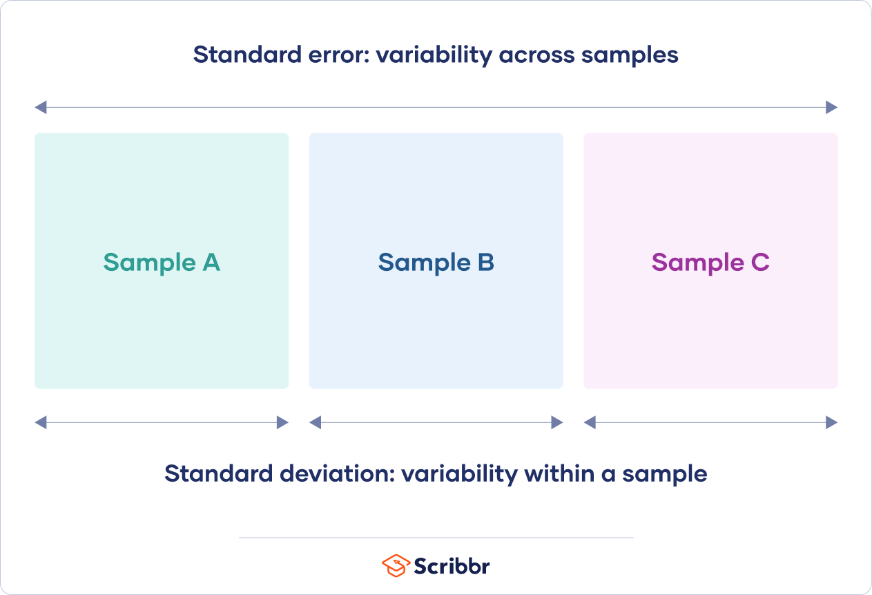
Standard error vs standard deviation
Standard error and standard deviation are both measures of variability:
- The standard deviation describes variability within a single sample.
- The standard error estimates the variability across multiple samples of a population.
The standard deviation is a descriptive statistic that can be calculated from sample data. In contrast, the standard error is an inferential statistic that can only be estimated (unless the real population parameter is known).
The standard deviation of the math scores is 180. This number reflects on average how much each score differs from the sample mean score of 550.
The standard error of the math scores, on the other hand, tells you how much the sample mean score of 550 differs from other sample mean scores, in samples of equal size, in the population of all test takers in the region.
What can proofreading do for your paper?
Scribbr editors not only correct grammar and spelling mistakes, but also strengthen your writing by making sure your paper is free of vague language, redundant words, and awkward phrasing.
See editing example
Standard error formula
The standard error of the mean is calculated using the standard deviation and the sample size.
From the formula, you’ll see that the sample size is inversely proportional to the standard error. This means that the larger the sample, the smaller the standard error, because the sample statistic will be closer to approaching the population parameter.
Different formulas are used depending on whether the population standard deviation is known. These formulas work for samples with more than 20 elements (n > 20).
When population parameters are known
When the population standard deviation is known, you can use it in the below formula to calculate standard error precisely.
| Formula | Explanation |
|---|---|
 |
|
 is standard error
 is population standard deviation
 is the number of elements in the sample
When population parameters are unknown
When the population standard deviation is unknown, you can use the below formula to only estimate standard error. This formula takes the sample standard deviation as a point estimate for the population standard deviation.
| Formula | Explanation |
|---|---|
 |
|
 is sample standard deviation
First, find the square root of your sample size (n).
| Formula | Calculation |
|---|---|
 |

|

Next, divide the sample standard deviation by the number you found in step one.
| Formula | Calculation |
|---|---|
|

|


The standard error of math SAT scores is 12.8.
How should you report the standard error?
You can report the standard error alongside the mean or in a confidence interval to communicate the uncertainty around the mean.
The best way to report the standard error is in a confidence interval because readers won’t have to do any additional math to come up with a meaningful interval.
A confidence interval is a range of values where an unknown population parameter is expected to lie most of the time, if you were to repeat your study with new random samples.
With a 95% confidence level, 95% of all sample means will be expected to lie within a confidence interval of ± 1.96 standard errors of the sample mean.
Based on random sampling, the true population parameter is also estimated to lie within this range with 95% confidence.
For a normally distributed characteristic, like SAT scores, 95% of all sample means fall within roughly 4 standard errors of the sample mean.
| Confidence interval formula | |
|---|---|
|
CI = x̄ ± (1.96 × SE) x̄ = sample mean = 550 |
|
| Lower limit | Upper limit |
|
x̄ − (1.96 × SE) 550 − (1.96 × 12.8) = 525 |
x̄ + (1.96 × SE) 550 + (1.96 × 12.8) = 575 |
With random sampling, a 95% CI [525 575] tells you that there is a 0.95 probability that the population mean math SAT score is between 525 and 575.
Other standard errors
Aside from the standard error of the mean (and other statistics), there are two other standard errors you might come across: the standard error of the estimate and the standard error of measurement.
The standard error of the estimate is related to regression analysis. This reflects the variability around the estimated regression line and the accuracy of the regression model. Using the standard error of the estimate, you can construct a confidence interval for the true regression coefficient.
The standard error of measurement is about the reliability of a measure. It indicates how variable the measurement error of a test is, and it’s often reported in standardized testing. The standard error of measurement can be used to create a confidence interval for the true score of an element or an individual.
Frequently asked questions about standard error
-
What is standard error?
-
The standard error of the mean, or simply standard error, indicates how different the population mean is likely to be from a sample mean. It tells you how much the sample mean would vary if you were to repeat a study using new samples from within a single population.
Cite this Scribbr article
If you want to cite this source, you can copy and paste the citation or click the “Cite this Scribbr article” button to automatically add the citation to our free Citation Generator.
Bhandari, P.
(2022, December 19). What Is Standard Error? | How to Calculate (Guide with Examples). Scribbr.
Retrieved February 9, 2023,
from https://www.scribbr.com/statistics/standard-error/
Is this article helpful?
You have already voted. Thanks 
Your vote is saved
Processing your vote…