Число обнаруживаемых или исправляемых ошибок.
При применении двоичных кодов учитывают
только дискретные искажения, при которых
единица переходит в нуль (1 → 0) или нуль
переходит в единицу (0 → 1). Переход 1 →
0 или 0 → 1 только в одном элементе кодовой
комбинации называют единичной ошибкой
(единичным искажением). В общем случае
под кратностью ошибки подразумевают
число позиций кодовой комбинации, на
которых под действием помехи одни
символы оказались заменёнными на другие.
Возможны двукратные (t= 2) и многократные (t> 2) искажения элементов в кодовой
комбинации в пределах 0 <t<n.
Минимальное кодовое расстояние является
основным параметром, характеризующим
корректирующие способности данного
кода. Если код используется только для
обнаружения ошибок кратностью t0,
то необходимо и достаточно, чтобы
минимальное кодовое расстояние было
равно
dmin
> t0
+ 1. (13.10)
В этом случае никакая комбинация из t0ошибок не может перевести одну разрешённую
кодовую комбинацию в другую разрешённую.
Таким образом, условие обнаружения всех
ошибок кратностьюt0можно записать в виде:
t0≤ dmin — 1. (13.11)
Чтобы можно было исправить все ошибки
кратностью tии менее, необходимо иметь минимальное
расстояние, удовлетворяющее условию:
![]() . (13.12)
. (13.12)
В этом случае любая кодовая комбинация
с числом ошибок tиотличается от каждой разрешённой
комбинации не менее чем вtи+ 1 позициях. Если условие (13.12) не выполнено,
возможен случай, когда ошибки кратностиtисказят переданную
комбинацию так, что она станет ближе к
одной из разрешённых комбинаций, чем к
переданной или даже перейдёт в другую
разрешённую комбинацию. В соответствии
с этим, условие исправления всех ошибок
кратностью не болееtиможно записать в виде:
tи
≤(dmin
— 1) / 2 . (13.13)
Из (13.10) и (13.12) следует, что если код
исправляет все ошибки кратностью tи,
то число ошибок, которые он может
обнаружить, равноt0= 2∙tи. Следует
отметить, что соотношения (13.10) и (13.12)
устанавливают лишь гарантированное
минимальное число обнаруживаемых или
исправляемых ошибок при заданномdminи не ограничивают возможность обнаружения
ошибок большей кратности. Например,
простейший код с проверкой на чётность
сdmin= 2 позволяет обнаруживать не только
одиночные ошибки, но и любое нечётное
число ошибок в пределахt0<n.
Корректирующие возможности кодов.
Вопрос о минимально необходимой
избыточности, при которой код обладает
нужными корректирующими свойствами,
является одним из важнейших в теории
кодирования. Этот вопрос до сих пор не
получил полного решения. В настоящее
время получен лишь ряд верхних и нижних
оценок (границ), которые устанавливают
связь между максимально возможным
минимальным расстоянием корректирующего
кода и его избыточностью.
Так, граница Плоткинадаёт верхнюю
границу кодового расстоянияdminпри заданном числе разрядовnв
кодовой комбинации и числе информационных
разрядовm, и для
двоичных кодов:
![]() (13.14)
(13.14)
или
![]() при
при![]() . (13.15)
. (13.15)
Верхняя граница Хеммингаустанавливает
максимально возможное число разрешённых
кодовых комбинаций (2m)
любого помехоустойчивого кода при
заданных значенияхnиdmin:
 , (13.16)
где
![]() —
—
число сочетаний изnэлементов поiэлементам.
Отсюда можно получить выражение для
оценки числа проверочных символов:
 . (13.17)
Для значений (dmin/n)
≤ 0,3 разница между границей Хемминга и
границей Плоткина сравнительно невелика.
Граница Варшамова-Гильбертадля
больших значенийnопределяет нижнюю
границу для числа проверочных разрядов,
необходимого для обеспечения заданного
кодового расстояния:
 . (13.18)
Отметим, что для некоторых частных
случаев Хемминг получил простые
соотношения, позволяющие определить
необходимое число проверочных символов:
![]() дляdmin= 3,
дляdmin= 3,
![]() дляdmin= 4.
дляdmin= 4.
Блочные коды с dmin= 3 и 4 в литературе обычно называют кодами
Хемминга.
Все приведенные выше оценки дают
представление о верхней границе числаdminпри фиксированных значенияхnиmили оценку снизу числа проверочных
символовkпри заданныхmиdmin.
Существующие методы построения избыточных
кодов решают в основном задачу нахождения
такого алгоритма кодирования и
декодирования, который позволял бы
наиболее просто построить и реализовать
код с заданным значением dmin.
Поэтому различные корректирующие коды
при одинаковыхdminсравниваются по сложности кодирующего
и декодирующего устройств. Этот критерий
является в ряде случаев определяющим
при выборе того или иного кода.
Соседние файлы в папке ЛБ_3
- #
- #
14.04.2015937 б70KodHemmig.m
- #
14.04.20150 б62ЛБ_3.exe
«Interleaver» redirects here. For the fiber-optic device, see optical interleaver.
In computing, telecommunication, information theory, and coding theory, forward error correction (FEC) or channel coding[1][2][3] is a technique used for controlling errors in data transmission over unreliable or noisy communication channels.
The central idea is that the sender encodes the message in a redundant way, most often by using an error correction code or error correcting code, (ECC).[4][5] The redundancy allows the receiver not only to detect errors that may occur anywhere in the message, but often to correct a limited number of errors. Therefore a reverse channel to request re-transmission may not be needed. The cost is a fixed, higher forward channel bandwidth.
The American mathematician Richard Hamming pioneered this field in the 1940s and invented the first error-correcting code in 1950: the Hamming (7,4) code.[5]
FEC can be applied in situations where re-transmissions are costly or impossible, such as one-way communication links or when transmitting to multiple receivers in multicast.
Long-latency connections also benefit; in the case of a satellite orbiting Uranus, retransmission due to errors can create a delay of five hours. FEC is widely used in modems and in cellular networks, as well.
FEC processing in a receiver may be applied to a digital bit stream or in the demodulation of a digitally modulated carrier. For the latter, FEC is an integral part of the initial analog-to-digital conversion in the receiver. The Viterbi decoder implements a soft-decision algorithm to demodulate digital data from an analog signal corrupted by noise. Many FEC decoders can also generate a bit-error rate (BER) signal which can be used as feedback to fine-tune the analog receiving electronics.
FEC information is added to mass storage (magnetic, optical and solid state/flash based) devices to enable recovery of corrupted data, and is used as ECC computer memory on systems that require special provisions for reliability.
The maximum proportion of errors or missing bits that can be corrected is determined by the design of the ECC, so different forward error correcting codes are suitable for different conditions. In general, a stronger code induces more redundancy that needs to be transmitted using the available bandwidth, which reduces the effective bit-rate while improving the received effective signal-to-noise ratio. The noisy-channel coding theorem of Claude Shannon can be used to compute the maximum achievable communication bandwidth for a given maximum acceptable error probability. This establishes bounds on the theoretical maximum information transfer rate of a channel with some given base noise level. However, the proof is not constructive, and hence gives no insight of how to build a capacity achieving code. After years of research, some advanced FEC systems like polar code[3] come very close to the theoretical maximum given by the Shannon channel capacity under the hypothesis of an infinite length frame.
How it works[edit]
ECC is accomplished by adding redundancy to the transmitted information using an algorithm. A redundant bit may be a complex function of many original information bits. The original information may or may not appear literally in the encoded output; codes that include the unmodified input in the output are systematic, while those that do not are non-systematic.
A simplistic example of ECC is to transmit each data bit 3 times, which is known as a (3,1) repetition code. Through a noisy channel, a receiver might see 8 versions of the output, see table below.
| Triplet received | Interpreted as |
|---|---|
| 000 | 0 (error-free) |
| 001 | 0 |
| 010 | 0 |
| 100 | 0 |
| 111 | 1 (error-free) |
| 110 | 1 |
| 101 | 1 |
| 011 | 1 |
This allows an error in any one of the three samples to be corrected by «majority vote», or «democratic voting». The correcting ability of this ECC is:
- Up to 1 bit of triplet in error, or
- up to 2 bits of triplet omitted (cases not shown in table).
Though simple to implement and widely used, this triple modular redundancy is a relatively inefficient ECC. Better ECC codes typically examine the last several tens or even the last several hundreds of previously received bits to determine how to decode the current small handful of bits (typically in groups of 2 to 8 bits).
Averaging noise to reduce errors[edit]
ECC could be said to work by «averaging noise»; since each data bit affects many transmitted symbols, the corruption of some symbols by noise usually allows the original user data to be extracted from the other, uncorrupted received symbols that also depend on the same user data.
- Because of this «risk-pooling» effect, digital communication systems that use ECC tend to work well above a certain minimum signal-to-noise ratio and not at all below it.
- This all-or-nothing tendency – the cliff effect – becomes more pronounced as stronger codes are used that more closely approach the theoretical Shannon limit.
- Interleaving ECC coded data can reduce the all or nothing properties of transmitted ECC codes when the channel errors tend to occur in bursts. However, this method has limits; it is best used on narrowband data.
Most telecommunication systems use a fixed channel code designed to tolerate the expected worst-case bit error rate, and then fail to work at all if the bit error rate is ever worse.
However, some systems adapt to the given channel error conditions: some instances of hybrid automatic repeat-request use a fixed ECC method as long as the ECC can handle the error rate, then switch to ARQ when the error rate gets too high;
adaptive modulation and coding uses a variety of ECC rates, adding more error-correction bits per packet when there are higher error rates in the channel, or taking them out when they are not needed.
Types of ECC[edit]

A block code (specifically a Hamming code) where redundant bits are added as a block to the end of the initial message
A continuous code convolutional code where redundant bits are added continuously into the structure of the code word
The two main categories of ECC codes are block codes and convolutional codes.
- Block codes work on fixed-size blocks (packets) of bits or symbols of predetermined size. Practical block codes can generally be hard-decoded in polynomial time to their block length.
- Convolutional codes work on bit or symbol streams of arbitrary length. They are most often soft decoded with the Viterbi algorithm, though other algorithms are sometimes used. Viterbi decoding allows asymptotically optimal decoding efficiency with increasing constraint length of the convolutional code, but at the expense of exponentially increasing complexity. A convolutional code that is terminated is also a ‘block code’ in that it encodes a block of input data, but the block size of a convolutional code is generally arbitrary, while block codes have a fixed size dictated by their algebraic characteristics. Types of termination for convolutional codes include «tail-biting» and «bit-flushing».
There are many types of block codes; Reed–Solomon coding is noteworthy for its widespread use in compact discs, DVDs, and hard disk drives. Other examples of classical block codes include Golay, BCH, Multidimensional parity, and Hamming codes.
Hamming ECC is commonly used to correct NAND flash memory errors.[6]
This provides single-bit error correction and 2-bit error detection.
Hamming codes are only suitable for more reliable single-level cell (SLC) NAND.
Denser multi-level cell (MLC) NAND may use multi-bit correcting ECC such as BCH or Reed–Solomon.[7][8] NOR Flash typically does not use any error correction.[7]
Classical block codes are usually decoded using hard-decision algorithms,[9] which means that for every input and output signal a hard decision is made whether it corresponds to a one or a zero bit. In contrast, convolutional codes are typically decoded using soft-decision algorithms like the Viterbi, MAP or BCJR algorithms, which process (discretized) analog signals, and which allow for much higher error-correction performance than hard-decision decoding.
Nearly all classical block codes apply the algebraic properties of finite fields. Hence classical block codes are often referred to as algebraic codes.
In contrast to classical block codes that often specify an error-detecting or error-correcting ability, many modern block codes such as LDPC codes lack such guarantees. Instead, modern codes are evaluated in terms of their bit error rates.
Most forward error correction codes correct only bit-flips, but not bit-insertions or bit-deletions.
In this setting, the Hamming distance is the appropriate way to measure the bit error rate.
A few forward error correction codes are designed to correct bit-insertions and bit-deletions, such as Marker Codes and Watermark Codes.
The Levenshtein distance is a more appropriate way to measure the bit error rate when using such codes.
[10]
Code-rate and the tradeoff between reliability and data rate[edit]
The fundamental principle of ECC is to add redundant bits in order to help the decoder to find out the true message that was encoded by the transmitter. The code-rate of a given ECC system is defined as the ratio between the number of information bits and the total number of bits (i.e., information plus redundancy bits) in a given communication package. The code-rate is hence a real number. A low code-rate close to zero implies a strong code that uses many redundant bits to achieve a good performance, while a large code-rate close to 1 implies a weak code.
The redundant bits that protect the information have to be transferred using the same communication resources that they are trying to protect. This causes a fundamental tradeoff between reliability and data rate.[11] In one extreme, a strong code (with low code-rate) can induce an important increase in the receiver SNR (signal-to-noise-ratio) decreasing the bit error rate, at the cost of reducing the effective data rate. On the other extreme, not using any ECC (i.e., a code-rate equal to 1) uses the full channel for information transfer purposes, at the cost of leaving the bits without any additional protection.
One interesting question is the following: how efficient in terms of information transfer can an ECC be that has a negligible decoding error rate? This question was answered by Claude Shannon with his second theorem, which says that the channel capacity is the maximum bit rate achievable by any ECC whose error rate tends to zero:[12] His proof relies on Gaussian random coding, which is not suitable to real-world applications. The upper bound given by Shannon’s work inspired a long journey in designing ECCs that can come close to the ultimate performance boundary. Various codes today can attain almost the Shannon limit. However, capacity achieving ECCs are usually extremely complex to implement.
The most popular ECCs have a trade-off between performance and computational complexity. Usually, their parameters give a range of possible code rates, which can be optimized depending on the scenario. Usually, this optimization is done in order to achieve a low decoding error probability while minimizing the impact to the data rate. Another criterion for optimizing the code rate is to balance low error rate and retransmissions number in order to the energy cost of the communication.[13]
Concatenated ECC codes for improved performance[edit]
Classical (algebraic) block codes and convolutional codes are frequently combined in concatenated coding schemes in which a short constraint-length Viterbi-decoded convolutional code does most of the work and a block code (usually Reed–Solomon) with larger symbol size and block length «mops up» any errors made by the convolutional decoder. Single pass decoding with this family of error correction codes can yield very low error rates, but for long range transmission conditions (like deep space) iterative decoding is recommended.
Concatenated codes have been standard practice in satellite and deep space communications since Voyager 2 first used the technique in its 1986 encounter with Uranus. The Galileo craft used iterative concatenated codes to compensate for the very high error rate conditions caused by having a failed antenna.
Low-density parity-check (LDPC)[edit]
Low-density parity-check (LDPC) codes are a class of highly efficient linear block
codes made from many single parity check (SPC) codes. They can provide performance very close to the channel capacity (the theoretical maximum) using an iterated soft-decision decoding approach, at linear time complexity in terms of their block length. Practical implementations rely heavily on decoding the constituent SPC codes in parallel.
LDPC codes were first introduced by Robert G. Gallager in his PhD thesis in 1960,
but due to the computational effort in implementing encoder and decoder and the introduction of Reed–Solomon codes,
they were mostly ignored until the 1990s.
LDPC codes are now used in many recent high-speed communication standards, such as DVB-S2 (Digital Video Broadcasting – Satellite – Second Generation), WiMAX (IEEE 802.16e standard for microwave communications), High-Speed Wireless LAN (IEEE 802.11n),[14] 10GBase-T Ethernet (802.3an) and G.hn/G.9960 (ITU-T Standard for networking over power lines, phone lines and coaxial cable). Other LDPC codes are standardized for wireless communication standards within 3GPP MBMS (see fountain codes).
Turbo codes[edit]
Turbo coding is an iterated soft-decoding scheme that combines two or more relatively simple convolutional codes and an interleaver to produce a block code that can perform to within a fraction of a decibel of the Shannon limit. Predating LDPC codes in terms of practical application, they now provide similar performance.
One of the earliest commercial applications of turbo coding was the CDMA2000 1x (TIA IS-2000) digital cellular technology developed by Qualcomm and sold by Verizon Wireless, Sprint, and other carriers. It is also used for the evolution of CDMA2000 1x specifically for Internet access, 1xEV-DO (TIA IS-856). Like 1x, EV-DO was developed by Qualcomm, and is sold by Verizon Wireless, Sprint, and other carriers (Verizon’s marketing name for 1xEV-DO is Broadband Access, Sprint’s consumer and business marketing names for 1xEV-DO are Power Vision and Mobile Broadband, respectively).
Local decoding and testing of codes[edit]
Sometimes it is only necessary to decode single bits of the message, or to check whether a given signal is a codeword, and do so without looking at the entire signal. This can make sense in a streaming setting, where codewords are too large to be classically decoded fast enough and where only a few bits of the message are of interest for now. Also such codes have become an important tool in computational complexity theory, e.g., for the design of probabilistically checkable proofs.
Locally decodable codes are error-correcting codes for which single bits of the message can be probabilistically recovered by only looking at a small (say constant) number of positions of a codeword, even after the codeword has been corrupted at some constant fraction of positions. Locally testable codes are error-correcting codes for which it can be checked probabilistically whether a signal is close to a codeword by only looking at a small number of positions of the signal.
Interleaving[edit]
«Interleaver» redirects here. For the fiber-optic device, see optical interleaver.

A short illustration of interleaving idea
Interleaving is frequently used in digital communication and storage systems to improve the performance of forward error correcting codes. Many communication channels are not memoryless: errors typically occur in bursts rather than independently. If the number of errors within a code word exceeds the error-correcting code’s capability, it fails to recover the original code word. Interleaving alleviates this problem by shuffling source symbols across several code words, thereby creating a more uniform distribution of errors.[15] Therefore, interleaving is widely used for burst error-correction.
The analysis of modern iterated codes, like turbo codes and LDPC codes, typically assumes an independent distribution of errors.[16] Systems using LDPC codes therefore typically employ additional interleaving across the symbols within a code word.[17]
For turbo codes, an interleaver is an integral component and its proper design is crucial for good performance.[15][18] The iterative decoding algorithm works best when there are not short cycles in the factor graph that represents the decoder; the interleaver is chosen to avoid short cycles.
Interleaver designs include:
- rectangular (or uniform) interleavers (similar to the method using skip factors described above)
- convolutional interleavers
- random interleavers (where the interleaver is a known random permutation)
- S-random interleaver (where the interleaver is a known random permutation with the constraint that no input symbols within distance S appear within a distance of S in the output).[19]
- a contention-free quadratic permutation polynomial (QPP).[20] An example of use is in the 3GPP Long Term Evolution mobile telecommunication standard.[21]
In multi-carrier communication systems, interleaving across carriers may be employed to provide frequency diversity, e.g., to mitigate frequency-selective fading or narrowband interference.[22]
Example[edit]
Transmission without interleaving:
Error-free message:                                 aaaabbbbccccddddeeeeffffgggg
Transmission with a burst error:                    aaaabbbbccc____deeeeffffgggg
Here, each group of the same letter represents a 4-bit one-bit error-correcting codeword. The codeword cccc is altered in one bit and can be corrected, but the codeword dddd is altered in three bits, so either it cannot be decoded at all or it might be decoded incorrectly.
With interleaving:
Error-free code words:                              aaaabbbbccccddddeeeeffffgggg
Interleaved:                                        abcdefgabcdefgabcdefgabcdefg
Transmission with a burst error:                    abcdefgabcd____bcdefgabcdefg
Received code words after deinterleaving:           aa_abbbbccccdddde_eef_ffg_gg
In each of the codewords «aaaa», «eeee», «ffff», and «gggg», only one bit is altered, so one-bit error-correcting code will decode everything correctly.
Transmission without interleaving:
Original transmitted sentence:                      ThisIsAnExampleOfInterleaving
Received sentence with a burst error:               ThisIs______pleOfInterleaving
The term «AnExample» ends up mostly unintelligible and difficult to correct.
With interleaving:
Transmitted sentence:                               ThisIsAnExampleOfInterleaving...
Error-free transmission:                            TIEpfeaghsxlIrv.iAaenli.snmOten.
Received sentence with a burst error:               TIEpfe______Irv.iAaenli.snmOten.
Received sentence after deinterleaving:             T_isI_AnE_amp_eOfInterle_vin_...
No word is completely lost and the missing letters can be recovered with minimal guesswork.
Disadvantages of interleaving[edit]
Use of interleaving techniques increases total delay. This is because the entire interleaved block must be received before the packets can be decoded.[23] Also interleavers hide the structure of errors; without an interleaver, more advanced decoding algorithms can take advantage of the error structure and achieve more reliable communication than a simpler decoder combined with an interleaver[citation needed]. An example of such an algorithm is based on neural network[24] structures.
Software for error-correcting codes[edit]
Simulating the behaviour of error-correcting codes (ECCs) in software is a common practice to design, validate and improve ECCs. The upcoming wireless 5G standard raises a new range of applications for the software ECCs: the Cloud Radio Access Networks (C-RAN) in a Software-defined radio (SDR) context. The idea is to directly use software ECCs in the communications. For instance in the 5G, the software ECCs could be located in the cloud and the antennas connected to this computing resources: improving this way the flexibility of the communication network and eventually increasing the energy efficiency of the system.
In this context, there are various available Open-source software listed below (non exhaustive).
- AFF3CT(A Fast Forward Error Correction Toolbox): a full communication chain in C++ (many supported codes like Turbo, LDPC, Polar codes, etc.), very fast and specialized on channel coding (can be used as a program for simulations or as a library for the SDR).
- IT++: a C++ library of classes and functions for linear algebra, numerical optimization, signal processing, communications, and statistics.
- OpenAir: implementation (in C) of the 3GPP specifications concerning the Evolved Packet Core Networks.
List of error-correcting codes[edit]
| Distance | Code |
|---|---|
| 2 (single-error detecting) | Parity |
| 3 (single-error correcting) | Triple modular redundancy |
| 3 (single-error correcting) | perfect Hamming such as Hamming(7,4) |
| 4 (SECDED) | Extended Hamming |
| 5 (double-error correcting) | |
| 6 (double-error correct-/triple error detect) | Nordstrom-Robinson code |
| 7 (three-error correcting) | perfect binary Golay code |
| 8 (TECFED) | extended binary Golay code |
- AN codes
- BCH code, which can be designed to correct any arbitrary number of errors per code block.
- Barker code used for radar, telemetry, ultra sound, Wifi, DSSS mobile phone networks, GPS etc.
- Berger code
- Constant-weight code
- Convolutional code
- Expander codes
- Group codes
- Golay codes, of which the Binary Golay code is of practical interest
- Goppa code, used in the McEliece cryptosystem
- Hadamard code
- Hagelbarger code
- Hamming code
- Latin square based code for non-white noise (prevalent for example in broadband over powerlines)
- Lexicographic code
- Linear Network Coding, a type of erasure correcting code across networks instead of point-to-point links
- Long code
- Low-density parity-check code, also known as Gallager code, as the archetype for sparse graph codes
- LT code, which is a near-optimal rateless erasure correcting code (Fountain code)
- m of n codes
- Nordstrom-Robinson code, used in Geometry and Group Theory[25]
- Online code, a near-optimal rateless erasure correcting code
- Polar code (coding theory)
- Raptor code, a near-optimal rateless erasure correcting code
- Reed–Solomon error correction
- Reed–Muller code
- Repeat-accumulate code
- Repetition codes, such as Triple modular redundancy
- Spinal code, a rateless, nonlinear code based on pseudo-random hash functions[26]
- Tornado code, a near-optimal erasure correcting code, and the precursor to Fountain codes
- Turbo code
- Walsh–Hadamard code
- Cyclic redundancy checks (CRCs) can correct 1-bit errors for messages at most
 bits long for optimal generator polynomials of degree , see Mathematics of cyclic redundancy checks#Bitfilters


See also[edit]
- Code rate
- Erasure codes
- Soft-decision decoder
- Burst error-correcting code
- Error detection and correction
- Error-correcting codes with feedback
References[edit]
- ^ Charles Wang; Dean Sklar; Diana Johnson (Winter 2001–2002). «Forward Error-Correction Coding». Crosslink. The Aerospace Corporation. 3 (1). Archived from the original on 14 March 2012. Retrieved 5 March 2006.
- ^ Charles Wang; Dean Sklar; Diana Johnson (Winter 2001–2002). «Forward Error-Correction Coding». Crosslink. The Aerospace Corporation. 3 (1). Archived from the original on 14 March 2012. Retrieved 5 March 2006.
How Forward Error-Correcting Codes Work]
- ^ a b Maunder, Robert (2016). «Overview of Channel Coding».
- ^ Glover, Neal; Dudley, Trent (1990). Practical Error Correction Design For Engineers (Revision 1.1, 2nd ed.). CO, USA: Cirrus Logic. ISBN 0-927239-00-0.
- ^ a b Hamming, Richard Wesley (April 1950). «Error Detecting and Error Correcting Codes». Bell System Technical Journal. USA: AT&T. 29 (2): 147–160. doi:10.1002/j.1538-7305.1950.tb00463.x. S2CID 61141773.
- ^ «Hamming codes for NAND flash memory devices» Archived 21 August 2016 at the Wayback Machine. EE Times-Asia. Apparently based on «Micron Technical Note TN-29-08: Hamming Codes for NAND Flash Memory Devices». 2005. Both say: «The Hamming algorithm is an industry-accepted method for error detection and correction in many SLC NAND flash-based applications.»
- ^ a b «What Types of ECC Should Be Used on Flash Memory?» (Application note). Spansion. 2011.
Both Reed–Solomon algorithm and BCH algorithm are common ECC choices for MLC NAND flash. … Hamming based block codes are the most commonly used ECC for SLC…. both Reed–Solomon and BCH are able to handle multiple errors and are widely used on MLC flash.
- ^ Jim Cooke (August 2007). «The Inconvenient Truths of NAND Flash Memory» (PDF). p. 28.
For SLC, a code with a correction threshold of 1 is sufficient. t=4 required … for MLC.
- ^ Baldi, M.; Chiaraluce, F. (2008). «A Simple Scheme for Belief Propagation Decoding of BCH and RS Codes in Multimedia Transmissions». International Journal of Digital Multimedia Broadcasting. 2008: 1–12. doi:10.1155/2008/957846.
- ^ Shah, Gaurav; Molina, Andres; Blaze, Matt (2006). «Keyboards and covert channels». USENIX. Retrieved 20 December 2018.
- ^ Tse, David; Viswanath, Pramod (2005), Fundamentals of Wireless Communication, Cambridge University Press, UK
- ^ Shannon, C. E. (1948). «A mathematical theory of communication» (PDF). Bell System Technical Journal. 27 (3–4): 379–423 & 623–656. doi:10.1002/j.1538-7305.1948.tb01338.x. hdl:11858/00-001M-0000-002C-4314-2.
- ^ Rosas, F.; Brante, G.; Souza, R. D.; Oberli, C. (2014). «Optimizing the code rate for achieving energy-efficient wireless communications». Proceedings of the IEEE Wireless Communications and Networking Conference (WCNC). pp. 775–780. doi:10.1109/WCNC.2014.6952166. ISBN 978-1-4799-3083-8.
- ^ IEEE Standard, section 20.3.11.6 «802.11n-2009» Archived 3 February 2013 at the Wayback Machine, IEEE, 29 October 2009, accessed 21 March 2011.
- ^ a b Vucetic, B.; Yuan, J. (2000). Turbo codes: principles and applications. Springer Verlag. ISBN 978-0-7923-7868-6.
- ^ Luby, Michael; Mitzenmacher, M.; Shokrollahi, A.; Spielman, D.; Stemann, V. (1997). «Practical Loss-Resilient Codes». Proc. 29th Annual Association for Computing Machinery (ACM) Symposium on Theory of Computation.
- ^ «Digital Video Broadcast (DVB); Second generation framing structure, channel coding and modulation systems for Broadcasting, Interactive Services, News Gathering and other satellite broadband applications (DVB-S2)». En 302 307. ETSI (V1.2.1). April 2009.
- ^ Andrews, K. S.; Divsalar, D.; Dolinar, S.; Hamkins, J.; Jones, C. R.; Pollara, F. (November 2007). «The Development of Turbo and LDPC Codes for Deep-Space Applications». Proceedings of the IEEE. 95 (11): 2142–2156. doi:10.1109/JPROC.2007.905132. S2CID 9289140.
- ^ Dolinar, S.; Divsalar, D. (15 August 1995). «Weight Distributions for Turbo Codes Using Random and Nonrandom Permutations». TDA Progress Report. 122: 42–122. Bibcode:1995TDAPR.122…56D. CiteSeerX 10.1.1.105.6640.
- ^ Takeshita, Oscar (2006). «Permutation Polynomial Interleavers: An Algebraic-Geometric Perspective». IEEE Transactions on Information Theory. 53 (6): 2116–2132. arXiv:cs/0601048. Bibcode:2006cs……..1048T. doi:10.1109/TIT.2007.896870. S2CID 660.
- ^ 3GPP TS 36.212, version 8.8.0, page 14
- ^ «Digital Video Broadcast (DVB); Frame structure, channel coding and modulation for a second generation digital terrestrial television broadcasting system (DVB-T2)». En 302 755. ETSI (V1.1.1). September 2009.
- ^ Techie (3 June 2010). «Explaining Interleaving». W3 Techie Blog. Retrieved 3 June 2010.
- ^ Krastanov, Stefan; Jiang, Liang (8 September 2017). «Deep Neural Network Probabilistic Decoder for Stabilizer Codes». Scientific Reports. 7 (1): 11003. arXiv:1705.09334. Bibcode:2017NatSR…711003K. doi:10.1038/s41598-017-11266-1. PMC 5591216. PMID 28887480.
- ^ Nordstrom, A.W.; Robinson, J.P. (1967), «An optimum nonlinear code», Information and Control, 11 (5–6): 613–616, doi:10.1016/S0019-9958(67)90835-2
- ^ Perry, Jonathan; Balakrishnan, Hari; Shah, Devavrat (2011). «Rateless Spinal Codes». Proceedings of the 10th ACM Workshop on Hot Topics in Networks. pp. 1–6. doi:10.1145/2070562.2070568. hdl:1721.1/79676. ISBN 9781450310598.
Further reading[edit]
- MacWilliams, Florence Jessiem; Sloane, Neil James Alexander (2007) [1977]. Written at AT&T Shannon Labs, Florham Park, New Jersey, USA. The Theory of Error-Correcting Codes. North-Holland Mathematical Library. Vol. 16 (digital print of 12th impression, 1st ed.). Amsterdam / London / New York / Tokyo: North-Holland / Elsevier BV. ISBN 978-0-444-85193-2. LCCN 76-41296. (xxii+762+6 pages)
- Clark, Jr., George C.; Cain, J. Bibb (1981). Error-Correction Coding for Digital Communications. New York, USA: Plenum Press. ISBN 0-306-40615-2.
- Arazi, Benjamin (1987). Swetman, Herb (ed.). A Commonsense Approach to the Theory of Error Correcting Codes. MIT Press Series in Computer Systems. Vol. 10 (1 ed.). Cambridge, Massachusetts, USA / London, UK: Massachusetts Institute of Technology. ISBN 0-262-01098-4. LCCN 87-21889. (x+2+208+4 pages)
- Wicker, Stephen B. (1995). Error Control Systems for Digital Communication and Storage. Englewood Cliffs, New Jersey, USA: Prentice-Hall. ISBN 0-13-200809-2.
- Wilson, Stephen G. (1996). Digital Modulation and Coding. Englewood Cliffs, New Jersey, USA: Prentice-Hall. ISBN 0-13-210071-1.
- «Error Correction Code in Single Level Cell NAND Flash memories» 2007-02-16
- «Error Correction Code in NAND Flash memories» 2004-11-29
- Observations on Errors, Corrections, & Trust of Dependent Systems, by James Hamilton, 2012-02-26
- Sphere Packings, Lattices and Groups, By J. H. Conway, Neil James Alexander Sloane, Springer Science & Business Media, 2013-03-09 – Mathematics – 682 pages.
External links[edit]
- Morelos-Zaragoza, Robert (2004). «The Correcting Codes (ECC) Page». Retrieved 5 March 2006.
- lpdec: library for LP decoding and related things (Python)
«Interleaver» redirects here. For the fiber-optic device, see optical interleaver.
In computing, telecommunication, information theory, and coding theory, forward error correction (FEC) or channel coding[1][2][3] is a technique used for controlling errors in data transmission over unreliable or noisy communication channels.
The central idea is that the sender encodes the message in a redundant way, most often by using an error correction code or error correcting code, (ECC).[4][5] The redundancy allows the receiver not only to detect errors that may occur anywhere in the message, but often to correct a limited number of errors. Therefore a reverse channel to request re-transmission may not be needed. The cost is a fixed, higher forward channel bandwidth.
The American mathematician Richard Hamming pioneered this field in the 1940s and invented the first error-correcting code in 1950: the Hamming (7,4) code.[5]
FEC can be applied in situations where re-transmissions are costly or impossible, such as one-way communication links or when transmitting to multiple receivers in multicast.
Long-latency connections also benefit; in the case of a satellite orbiting Uranus, retransmission due to errors can create a delay of five hours. FEC is widely used in modems and in cellular networks, as well.
FEC processing in a receiver may be applied to a digital bit stream or in the demodulation of a digitally modulated carrier. For the latter, FEC is an integral part of the initial analog-to-digital conversion in the receiver. The Viterbi decoder implements a soft-decision algorithm to demodulate digital data from an analog signal corrupted by noise. Many FEC decoders can also generate a bit-error rate (BER) signal which can be used as feedback to fine-tune the analog receiving electronics.
FEC information is added to mass storage (magnetic, optical and solid state/flash based) devices to enable recovery of corrupted data, and is used as ECC computer memory on systems that require special provisions for reliability.
The maximum proportion of errors or missing bits that can be corrected is determined by the design of the ECC, so different forward error correcting codes are suitable for different conditions. In general, a stronger code induces more redundancy that needs to be transmitted using the available bandwidth, which reduces the effective bit-rate while improving the received effective signal-to-noise ratio. The noisy-channel coding theorem of Claude Shannon can be used to compute the maximum achievable communication bandwidth for a given maximum acceptable error probability. This establishes bounds on the theoretical maximum information transfer rate of a channel with some given base noise level. However, the proof is not constructive, and hence gives no insight of how to build a capacity achieving code. After years of research, some advanced FEC systems like polar code[3] come very close to the theoretical maximum given by the Shannon channel capacity under the hypothesis of an infinite length frame.
How it works[edit]
ECC is accomplished by adding redundancy to the transmitted information using an algorithm. A redundant bit may be a complex function of many original information bits. The original information may or may not appear literally in the encoded output; codes that include the unmodified input in the output are systematic, while those that do not are non-systematic.
A simplistic example of ECC is to transmit each data bit 3 times, which is known as a (3,1) repetition code. Through a noisy channel, a receiver might see 8 versions of the output, see table below.
| Triplet received | Interpreted as |
|---|---|
| 000 | 0 (error-free) |
| 001 | 0 |
| 010 | 0 |
| 100 | 0 |
| 111 | 1 (error-free) |
| 110 | 1 |
| 101 | 1 |
| 011 | 1 |
This allows an error in any one of the three samples to be corrected by «majority vote», or «democratic voting». The correcting ability of this ECC is:
- Up to 1 bit of triplet in error, or
- up to 2 bits of triplet omitted (cases not shown in table).
Though simple to implement and widely used, this triple modular redundancy is a relatively inefficient ECC. Better ECC codes typically examine the last several tens or even the last several hundreds of previously received bits to determine how to decode the current small handful of bits (typically in groups of 2 to 8 bits).
Averaging noise to reduce errors[edit]
ECC could be said to work by «averaging noise»; since each data bit affects many transmitted symbols, the corruption of some symbols by noise usually allows the original user data to be extracted from the other, uncorrupted received symbols that also depend on the same user data.
- Because of this «risk-pooling» effect, digital communication systems that use ECC tend to work well above a certain minimum signal-to-noise ratio and not at all below it.
- This all-or-nothing tendency – the cliff effect – becomes more pronounced as stronger codes are used that more closely approach the theoretical Shannon limit.
- Interleaving ECC coded data can reduce the all or nothing properties of transmitted ECC codes when the channel errors tend to occur in bursts. However, this method has limits; it is best used on narrowband data.
Most telecommunication systems use a fixed channel code designed to tolerate the expected worst-case bit error rate, and then fail to work at all if the bit error rate is ever worse.
However, some systems adapt to the given channel error conditions: some instances of hybrid automatic repeat-request use a fixed ECC method as long as the ECC can handle the error rate, then switch to ARQ when the error rate gets too high;
adaptive modulation and coding uses a variety of ECC rates, adding more error-correction bits per packet when there are higher error rates in the channel, or taking them out when they are not needed.
Types of ECC[edit]
A block code (specifically a Hamming code) where redundant bits are added as a block to the end of the initial message
A continuous code convolutional code where redundant bits are added continuously into the structure of the code word
The two main categories of ECC codes are block codes and convolutional codes.
- Block codes work on fixed-size blocks (packets) of bits or symbols of predetermined size. Practical block codes can generally be hard-decoded in polynomial time to their block length.
- Convolutional codes work on bit or symbol streams of arbitrary length. They are most often soft decoded with the Viterbi algorithm, though other algorithms are sometimes used. Viterbi decoding allows asymptotically optimal decoding efficiency with increasing constraint length of the convolutional code, but at the expense of exponentially increasing complexity. A convolutional code that is terminated is also a ‘block code’ in that it encodes a block of input data, but the block size of a convolutional code is generally arbitrary, while block codes have a fixed size dictated by their algebraic characteristics. Types of termination for convolutional codes include «tail-biting» and «bit-flushing».
There are many types of block codes; Reed–Solomon coding is noteworthy for its widespread use in compact discs, DVDs, and hard disk drives. Other examples of classical block codes include Golay, BCH, Multidimensional parity, and Hamming codes.
Hamming ECC is commonly used to correct NAND flash memory errors.[6]
This provides single-bit error correction and 2-bit error detection.
Hamming codes are only suitable for more reliable single-level cell (SLC) NAND.
Denser multi-level cell (MLC) NAND may use multi-bit correcting ECC such as BCH or Reed–Solomon.[7][8] NOR Flash typically does not use any error correction.[7]
Classical block codes are usually decoded using hard-decision algorithms,[9] which means that for every input and output signal a hard decision is made whether it corresponds to a one or a zero bit. In contrast, convolutional codes are typically decoded using soft-decision algorithms like the Viterbi, MAP or BCJR algorithms, which process (discretized) analog signals, and which allow for much higher error-correction performance than hard-decision decoding.
Nearly all classical block codes apply the algebraic properties of finite fields. Hence classical block codes are often referred to as algebraic codes.
In contrast to classical block codes that often specify an error-detecting or error-correcting ability, many modern block codes such as LDPC codes lack such guarantees. Instead, modern codes are evaluated in terms of their bit error rates.
Most forward error correction codes correct only bit-flips, but not bit-insertions or bit-deletions.
In this setting, the Hamming distance is the appropriate way to measure the bit error rate.
A few forward error correction codes are designed to correct bit-insertions and bit-deletions, such as Marker Codes and Watermark Codes.
The Levenshtein distance is a more appropriate way to measure the bit error rate when using such codes.
[10]
Code-rate and the tradeoff between reliability and data rate[edit]
The fundamental principle of ECC is to add redundant bits in order to help the decoder to find out the true message that was encoded by the transmitter. The code-rate of a given ECC system is defined as the ratio between the number of information bits and the total number of bits (i.e., information plus redundancy bits) in a given communication package. The code-rate is hence a real number. A low code-rate close to zero implies a strong code that uses many redundant bits to achieve a good performance, while a large code-rate close to 1 implies a weak code.
The redundant bits that protect the information have to be transferred using the same communication resources that they are trying to protect. This causes a fundamental tradeoff between reliability and data rate.[11] In one extreme, a strong code (with low code-rate) can induce an important increase in the receiver SNR (signal-to-noise-ratio) decreasing the bit error rate, at the cost of reducing the effective data rate. On the other extreme, not using any ECC (i.e., a code-rate equal to 1) uses the full channel for information transfer purposes, at the cost of leaving the bits without any additional protection.
One interesting question is the following: how efficient in terms of information transfer can an ECC be that has a negligible decoding error rate? This question was answered by Claude Shannon with his second theorem, which says that the channel capacity is the maximum bit rate achievable by any ECC whose error rate tends to zero:[12] His proof relies on Gaussian random coding, which is not suitable to real-world applications. The upper bound given by Shannon’s work inspired a long journey in designing ECCs that can come close to the ultimate performance boundary. Various codes today can attain almost the Shannon limit. However, capacity achieving ECCs are usually extremely complex to implement.
The most popular ECCs have a trade-off between performance and computational complexity. Usually, their parameters give a range of possible code rates, which can be optimized depending on the scenario. Usually, this optimization is done in order to achieve a low decoding error probability while minimizing the impact to the data rate. Another criterion for optimizing the code rate is to balance low error rate and retransmissions number in order to the energy cost of the communication.[13]
Concatenated ECC codes for improved performance[edit]
Classical (algebraic) block codes and convolutional codes are frequently combined in concatenated coding schemes in which a short constraint-length Viterbi-decoded convolutional code does most of the work and a block code (usually Reed–Solomon) with larger symbol size and block length «mops up» any errors made by the convolutional decoder. Single pass decoding with this family of error correction codes can yield very low error rates, but for long range transmission conditions (like deep space) iterative decoding is recommended.
Concatenated codes have been standard practice in satellite and deep space communications since Voyager 2 first used the technique in its 1986 encounter with Uranus. The Galileo craft used iterative concatenated codes to compensate for the very high error rate conditions caused by having a failed antenna.
Low-density parity-check (LDPC)[edit]
Low-density parity-check (LDPC) codes are a class of highly efficient linear block
codes made from many single parity check (SPC) codes. They can provide performance very close to the channel capacity (the theoretical maximum) using an iterated soft-decision decoding approach, at linear time complexity in terms of their block length. Practical implementations rely heavily on decoding the constituent SPC codes in parallel.
LDPC codes were first introduced by Robert G. Gallager in his PhD thesis in 1960,
but due to the computational effort in implementing encoder and decoder and the introduction of Reed–Solomon codes,
they were mostly ignored until the 1990s.
LDPC codes are now used in many recent high-speed communication standards, such as DVB-S2 (Digital Video Broadcasting – Satellite – Second Generation), WiMAX (IEEE 802.16e standard for microwave communications), High-Speed Wireless LAN (IEEE 802.11n),[14] 10GBase-T Ethernet (802.3an) and G.hn/G.9960 (ITU-T Standard for networking over power lines, phone lines and coaxial cable). Other LDPC codes are standardized for wireless communication standards within 3GPP MBMS (see fountain codes).
Turbo codes[edit]
Turbo coding is an iterated soft-decoding scheme that combines two or more relatively simple convolutional codes and an interleaver to produce a block code that can perform to within a fraction of a decibel of the Shannon limit. Predating LDPC codes in terms of practical application, they now provide similar performance.
One of the earliest commercial applications of turbo coding was the CDMA2000 1x (TIA IS-2000) digital cellular technology developed by Qualcomm and sold by Verizon Wireless, Sprint, and other carriers. It is also used for the evolution of CDMA2000 1x specifically for Internet access, 1xEV-DO (TIA IS-856). Like 1x, EV-DO was developed by Qualcomm, and is sold by Verizon Wireless, Sprint, and other carriers (Verizon’s marketing name for 1xEV-DO is Broadband Access, Sprint’s consumer and business marketing names for 1xEV-DO are Power Vision and Mobile Broadband, respectively).
Local decoding and testing of codes[edit]
Sometimes it is only necessary to decode single bits of the message, or to check whether a given signal is a codeword, and do so without looking at the entire signal. This can make sense in a streaming setting, where codewords are too large to be classically decoded fast enough and where only a few bits of the message are of interest for now. Also such codes have become an important tool in computational complexity theory, e.g., for the design of probabilistically checkable proofs.
Locally decodable codes are error-correcting codes for which single bits of the message can be probabilistically recovered by only looking at a small (say constant) number of positions of a codeword, even after the codeword has been corrupted at some constant fraction of positions. Locally testable codes are error-correcting codes for which it can be checked probabilistically whether a signal is close to a codeword by only looking at a small number of positions of the signal.
Interleaving[edit]
«Interleaver» redirects here. For the fiber-optic device, see optical interleaver.
A short illustration of interleaving idea
Interleaving is frequently used in digital communication and storage systems to improve the performance of forward error correcting codes. Many communication channels are not memoryless: errors typically occur in bursts rather than independently. If the number of errors within a code word exceeds the error-correcting code’s capability, it fails to recover the original code word. Interleaving alleviates this problem by shuffling source symbols across several code words, thereby creating a more uniform distribution of errors.[15] Therefore, interleaving is widely used for burst error-correction.
The analysis of modern iterated codes, like turbo codes and LDPC codes, typically assumes an independent distribution of errors.[16] Systems using LDPC codes therefore typically employ additional interleaving across the symbols within a code word.[17]
For turbo codes, an interleaver is an integral component and its proper design is crucial for good performance.[15][18] The iterative decoding algorithm works best when there are not short cycles in the factor graph that represents the decoder; the interleaver is chosen to avoid short cycles.
Interleaver designs include:
- rectangular (or uniform) interleavers (similar to the method using skip factors described above)
- convolutional interleavers
- random interleavers (where the interleaver is a known random permutation)
- S-random interleaver (where the interleaver is a known random permutation with the constraint that no input symbols within distance S appear within a distance of S in the output).[19]
- a contention-free quadratic permutation polynomial (QPP).[20] An example of use is in the 3GPP Long Term Evolution mobile telecommunication standard.[21]
In multi-carrier communication systems, interleaving across carriers may be employed to provide frequency diversity, e.g., to mitigate frequency-selective fading or narrowband interference.[22]
Example[edit]
Transmission without interleaving:
Error-free message:                                 aaaabbbbccccddddeeeeffffgggg
Transmission with a burst error:                    aaaabbbbccc____deeeeffffgggg
Here, each group of the same letter represents a 4-bit one-bit error-correcting codeword. The codeword cccc is altered in one bit and can be corrected, but the codeword dddd is altered in three bits, so either it cannot be decoded at all or it might be decoded incorrectly.
With interleaving:
Error-free code words:                              aaaabbbbccccddddeeeeffffgggg
Interleaved:                                        abcdefgabcdefgabcdefgabcdefg
Transmission with a burst error:                    abcdefgabcd____bcdefgabcdefg
Received code words after deinterleaving:           aa_abbbbccccdddde_eef_ffg_gg
In each of the codewords «aaaa», «eeee», «ffff», and «gggg», only one bit is altered, so one-bit error-correcting code will decode everything correctly.
Transmission without interleaving:
Original transmitted sentence:                      ThisIsAnExampleOfInterleaving
Received sentence with a burst error:               ThisIs______pleOfInterleaving
The term «AnExample» ends up mostly unintelligible and difficult to correct.
With interleaving:
Transmitted sentence:                               ThisIsAnExampleOfInterleaving...
Error-free transmission:                            TIEpfeaghsxlIrv.iAaenli.snmOten.
Received sentence with a burst error:               TIEpfe______Irv.iAaenli.snmOten.
Received sentence after deinterleaving:             T_isI_AnE_amp_eOfInterle_vin_...
No word is completely lost and the missing letters can be recovered with minimal guesswork.
Disadvantages of interleaving[edit]
Use of interleaving techniques increases total delay. This is because the entire interleaved block must be received before the packets can be decoded.[23] Also interleavers hide the structure of errors; without an interleaver, more advanced decoding algorithms can take advantage of the error structure and achieve more reliable communication than a simpler decoder combined with an interleaver[citation needed]. An example of such an algorithm is based on neural network[24] structures.
Software for error-correcting codes[edit]
Simulating the behaviour of error-correcting codes (ECCs) in software is a common practice to design, validate and improve ECCs. The upcoming wireless 5G standard raises a new range of applications for the software ECCs: the Cloud Radio Access Networks (C-RAN) in a Software-defined radio (SDR) context. The idea is to directly use software ECCs in the communications. For instance in the 5G, the software ECCs could be located in the cloud and the antennas connected to this computing resources: improving this way the flexibility of the communication network and eventually increasing the energy efficiency of the system.
In this context, there are various available Open-source software listed below (non exhaustive).
- AFF3CT(A Fast Forward Error Correction Toolbox): a full communication chain in C++ (many supported codes like Turbo, LDPC, Polar codes, etc.), very fast and specialized on channel coding (can be used as a program for simulations or as a library for the SDR).
- IT++: a C++ library of classes and functions for linear algebra, numerical optimization, signal processing, communications, and statistics.
- OpenAir: implementation (in C) of the 3GPP specifications concerning the Evolved Packet Core Networks.
List of error-correcting codes[edit]
| Distance | Code |
|---|---|
| 2 (single-error detecting) | Parity |
| 3 (single-error correcting) | Triple modular redundancy |
| 3 (single-error correcting) | perfect Hamming such as Hamming(7,4) |
| 4 (SECDED) | Extended Hamming |
| 5 (double-error correcting) | |
| 6 (double-error correct-/triple error detect) | Nordstrom-Robinson code |
| 7 (three-error correcting) | perfect binary Golay code |
| 8 (TECFED) | extended binary Golay code |
- AN codes
- BCH code, which can be designed to correct any arbitrary number of errors per code block.
- Barker code used for radar, telemetry, ultra sound, Wifi, DSSS mobile phone networks, GPS etc.
- Berger code
- Constant-weight code
- Convolutional code
- Expander codes
- Group codes
- Golay codes, of which the Binary Golay code is of practical interest
- Goppa code, used in the McEliece cryptosystem
- Hadamard code
- Hagelbarger code
- Hamming code
- Latin square based code for non-white noise (prevalent for example in broadband over powerlines)
- Lexicographic code
- Linear Network Coding, a type of erasure correcting code across networks instead of point-to-point links
- Long code
- Low-density parity-check code, also known as Gallager code, as the archetype for sparse graph codes
- LT code, which is a near-optimal rateless erasure correcting code (Fountain code)
- m of n codes
- Nordstrom-Robinson code, used in Geometry and Group Theory[25]
- Online code, a near-optimal rateless erasure correcting code
- Polar code (coding theory)
- Raptor code, a near-optimal rateless erasure correcting code
- Reed–Solomon error correction
- Reed–Muller code
- Repeat-accumulate code
- Repetition codes, such as Triple modular redundancy
- Spinal code, a rateless, nonlinear code based on pseudo-random hash functions[26]
- Tornado code, a near-optimal erasure correcting code, and the precursor to Fountain codes
- Turbo code
- Walsh–Hadamard code
- Cyclic redundancy checks (CRCs) can correct 1-bit errors for messages at most bits long for optimal generator polynomials of degree , see Mathematics of cyclic redundancy checks#Bitfilters
See also[edit]
- Code rate
- Erasure codes
- Soft-decision decoder
- Burst error-correcting code
- Error detection and correction
- Error-correcting codes with feedback
References[edit]
- ^ Charles Wang; Dean Sklar; Diana Johnson (Winter 2001–2002). «Forward Error-Correction Coding». Crosslink. The Aerospace Corporation. 3 (1). Archived from the original on 14 March 2012. Retrieved 5 March 2006.
- ^ Charles Wang; Dean Sklar; Diana Johnson (Winter 2001–2002). «Forward Error-Correction Coding». Crosslink. The Aerospace Corporation. 3 (1). Archived from the original on 14 March 2012. Retrieved 5 March 2006.
How Forward Error-Correcting Codes Work]
- ^ a b Maunder, Robert (2016). «Overview of Channel Coding».
- ^ Glover, Neal; Dudley, Trent (1990). Practical Error Correction Design For Engineers (Revision 1.1, 2nd ed.). CO, USA: Cirrus Logic. ISBN 0-927239-00-0.
- ^ a b Hamming, Richard Wesley (April 1950). «Error Detecting and Error Correcting Codes». Bell System Technical Journal. USA: AT&T. 29 (2): 147–160. doi:10.1002/j.1538-7305.1950.tb00463.x. S2CID 61141773.
- ^ «Hamming codes for NAND flash memory devices» Archived 21 August 2016 at the Wayback Machine. EE Times-Asia. Apparently based on «Micron Technical Note TN-29-08: Hamming Codes for NAND Flash Memory Devices». 2005. Both say: «The Hamming algorithm is an industry-accepted method for error detection and correction in many SLC NAND flash-based applications.»
- ^ a b «What Types of ECC Should Be Used on Flash Memory?» (Application note). Spansion. 2011.
Both Reed–Solomon algorithm and BCH algorithm are common ECC choices for MLC NAND flash. … Hamming based block codes are the most commonly used ECC for SLC…. both Reed–Solomon and BCH are able to handle multiple errors and are widely used on MLC flash.
- ^ Jim Cooke (August 2007). «The Inconvenient Truths of NAND Flash Memory» (PDF). p. 28.
For SLC, a code with a correction threshold of 1 is sufficient. t=4 required … for MLC.
- ^ Baldi, M.; Chiaraluce, F. (2008). «A Simple Scheme for Belief Propagation Decoding of BCH and RS Codes in Multimedia Transmissions». International Journal of Digital Multimedia Broadcasting. 2008: 1–12. doi:10.1155/2008/957846.
- ^ Shah, Gaurav; Molina, Andres; Blaze, Matt (2006). «Keyboards and covert channels». USENIX. Retrieved 20 December 2018.
- ^ Tse, David; Viswanath, Pramod (2005), Fundamentals of Wireless Communication, Cambridge University Press, UK
- ^ Shannon, C. E. (1948). «A mathematical theory of communication» (PDF). Bell System Technical Journal. 27 (3–4): 379–423 & 623–656. doi:10.1002/j.1538-7305.1948.tb01338.x. hdl:11858/00-001M-0000-002C-4314-2.
- ^ Rosas, F.; Brante, G.; Souza, R. D.; Oberli, C. (2014). «Optimizing the code rate for achieving energy-efficient wireless communications». Proceedings of the IEEE Wireless Communications and Networking Conference (WCNC). pp. 775–780. doi:10.1109/WCNC.2014.6952166. ISBN 978-1-4799-3083-8.
- ^ IEEE Standard, section 20.3.11.6 «802.11n-2009» Archived 3 February 2013 at the Wayback Machine, IEEE, 29 October 2009, accessed 21 March 2011.
- ^ a b Vucetic, B.; Yuan, J. (2000). Turbo codes: principles and applications. Springer Verlag. ISBN 978-0-7923-7868-6.
- ^ Luby, Michael; Mitzenmacher, M.; Shokrollahi, A.; Spielman, D.; Stemann, V. (1997). «Practical Loss-Resilient Codes». Proc. 29th Annual Association for Computing Machinery (ACM) Symposium on Theory of Computation.
- ^ «Digital Video Broadcast (DVB); Second generation framing structure, channel coding and modulation systems for Broadcasting, Interactive Services, News Gathering and other satellite broadband applications (DVB-S2)». En 302 307. ETSI (V1.2.1). April 2009.
- ^ Andrews, K. S.; Divsalar, D.; Dolinar, S.; Hamkins, J.; Jones, C. R.; Pollara, F. (November 2007). «The Development of Turbo and LDPC Codes for Deep-Space Applications». Proceedings of the IEEE. 95 (11): 2142–2156. doi:10.1109/JPROC.2007.905132. S2CID 9289140.
- ^ Dolinar, S.; Divsalar, D. (15 August 1995). «Weight Distributions for Turbo Codes Using Random and Nonrandom Permutations». TDA Progress Report. 122: 42–122. Bibcode:1995TDAPR.122…56D. CiteSeerX 10.1.1.105.6640.
- ^ Takeshita, Oscar (2006). «Permutation Polynomial Interleavers: An Algebraic-Geometric Perspective». IEEE Transactions on Information Theory. 53 (6): 2116–2132. arXiv:cs/0601048. Bibcode:2006cs……..1048T. doi:10.1109/TIT.2007.896870. S2CID 660.
- ^ 3GPP TS 36.212, version 8.8.0, page 14
- ^ «Digital Video Broadcast (DVB); Frame structure, channel coding and modulation for a second generation digital terrestrial television broadcasting system (DVB-T2)». En 302 755. ETSI (V1.1.1). September 2009.
- ^ Techie (3 June 2010). «Explaining Interleaving». W3 Techie Blog. Retrieved 3 June 2010.
- ^ Krastanov, Stefan; Jiang, Liang (8 September 2017). «Deep Neural Network Probabilistic Decoder for Stabilizer Codes». Scientific Reports. 7 (1): 11003. arXiv:1705.09334. Bibcode:2017NatSR…711003K. doi:10.1038/s41598-017-11266-1. PMC 5591216. PMID 28887480.
- ^ Nordstrom, A.W.; Robinson, J.P. (1967), «An optimum nonlinear code», Information and Control, 11 (5–6): 613–616, doi:10.1016/S0019-9958(67)90835-2
- ^ Perry, Jonathan; Balakrishnan, Hari; Shah, Devavrat (2011). «Rateless Spinal Codes». Proceedings of the 10th ACM Workshop on Hot Topics in Networks. pp. 1–6. doi:10.1145/2070562.2070568. hdl:1721.1/79676. ISBN 9781450310598.
Further reading[edit]
- MacWilliams, Florence Jessiem; Sloane, Neil James Alexander (2007) [1977]. Written at AT&T Shannon Labs, Florham Park, New Jersey, USA. The Theory of Error-Correcting Codes. North-Holland Mathematical Library. Vol. 16 (digital print of 12th impression, 1st ed.). Amsterdam / London / New York / Tokyo: North-Holland / Elsevier BV. ISBN 978-0-444-85193-2. LCCN 76-41296. (xxii+762+6 pages)
- Clark, Jr., George C.; Cain, J. Bibb (1981). Error-Correction Coding for Digital Communications. New York, USA: Plenum Press. ISBN 0-306-40615-2.
- Arazi, Benjamin (1987). Swetman, Herb (ed.). A Commonsense Approach to the Theory of Error Correcting Codes. MIT Press Series in Computer Systems. Vol. 10 (1 ed.). Cambridge, Massachusetts, USA / London, UK: Massachusetts Institute of Technology. ISBN 0-262-01098-4. LCCN 87-21889. (x+2+208+4 pages)
- Wicker, Stephen B. (1995). Error Control Systems for Digital Communication and Storage. Englewood Cliffs, New Jersey, USA: Prentice-Hall. ISBN 0-13-200809-2.
- Wilson, Stephen G. (1996). Digital Modulation and Coding. Englewood Cliffs, New Jersey, USA: Prentice-Hall. ISBN 0-13-210071-1.
- «Error Correction Code in Single Level Cell NAND Flash memories» 2007-02-16
- «Error Correction Code in NAND Flash memories» 2004-11-29
- Observations on Errors, Corrections, & Trust of Dependent Systems, by James Hamilton, 2012-02-26
- Sphere Packings, Lattices and Groups, By J. H. Conway, Neil James Alexander Sloane, Springer Science & Business Media, 2013-03-09 – Mathematics – 682 pages.
External links[edit]
- Morelos-Zaragoza, Robert (2004). «The Correcting Codes (ECC) Page». Retrieved 5 March 2006.
- lpdec: library for LP decoding and related things (Python)
Назначение помехоустойчивого кодирования – защита информации от помех и ошибок при передаче и хранении информации. Помехоустойчивое кодирование необходимо для устранения ошибок, которые возникают в процессе передачи, хранения информации. При передачи информации по каналу связи возникают помехи, ошибки и небольшая часть информации теряется.

Без использования помехоустойчивого кодирования было бы невозможно передавать большие объемы информации (файлы), т.к. в любой системе передачи и хранении информации неизбежно возникают ошибки.
Рассмотрим пример CD диска. Там информация хранится прямо на поверхности диска, в углублениях, из-за того, что все дорожки на поверхности, часто диск хватаем пальцами, елозим по столу и из-за этого без помехоустойчивого кодирования, информацию извлечь не получится.
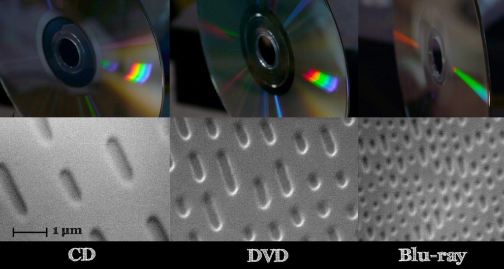
Использование кодирования позволяет извлекать информацию без потерь даже с поврежденного CD/DVD диска, когда какая либо область становится недоступной для считывания.
В зависимости от того, используется в системе обнаружение или исправление ошибок с помощью помехоустойчивого кода, различают следующие варианты:
- запрос повторной передачи (Automatic Repeat reQuest, ARQ): с помощью помехоустойчивого кода выполняется только обнаружение ошибок, при их наличии производится запрос на повторную передачу пакета данных;
- прямое исправление ошибок (Forward Error Correction, FEC): производится декодирование помехоустойчивого кода, т. е. исправление ошибок с его помощью.
Возможен также гибридный вариант, чтобы лишний раз не гонять информацию по каналу связи, например получили пакет информации, попробовали его исправить, и если не смогли исправить, тогда отправляется запрос на повторную передачу.
Исправление ошибок в помехоустойчивом кодировании
Любое помехоустойчивое кодирование добавляет избыточность, за счет чего и появляется возможность восстановить информацию при частичной потере данных в канале связи (носителе информации при хранении). В случае эффективного кодирования убирали избыточность, а в помехоустойчивом кодировании добавляется контролируемая избыточность.
Простейший пример – мажоритарный метод, он же многократная передача, в котором один символ передается многократно, а на приемной стороне принимается решение о том символе, количество которых больше.
Допустим есть 4 символа информации, А, B, С,D, и эту информацию повторяем несколько раз. В процессе передачи информации по каналу связи, где-то возникла ошибка. Есть три пакета (A1B1C1D1|A2B2C2D2|A3B3C3D3), которые должны нести одну и ту же информацию.

Но из картинки справа, видно, что второй символ (B1 и C1) они отличаются друг от друга, хотя должны были быть одинаковыми. То что они отличаются, говорит о том, что есть ошибка.
Необходимо найти ошибку с помощью голосования, каких символов больше, символов В или символов С? Явно символов В больше, чем символов С, соответственно принимаем решение, что передавался символ В, а символ С ошибочный.
Для исправления ошибок нужно, как минимум 3 пакета информации, для обнаружения, как минимум 2 пакета информации.
Параметры помехоустойчивого кодирования
Первый параметр, скорость кода R характеризует долю информационных («полезных») данных в сообщении и определяется выражением: R=k/n=k/m+k
- где n – количество символов закодированного сообщения (результата кодирования);
- m – количество проверочных символов, добавляемых при кодировании;
- k – количество информационных символов.
Параметры n и k часто приводят вместе с наименованием кода для его однозначной идентификации. Например, код Хэмминга (7,4) значит, что на вход кодера приходит 4 символа, на выходе 7 символов, Рида-Соломона (15, 11) и т.д.
Второй параметр, кратность обнаруживаемых ошибок – количество ошибочных символов, которые код может обнаружить.
Третий параметр, кратность исправляемых ошибок – количество ошибочных символов, которые код может исправить (обозначается буквой t).
Контроль чётности
Самый простой метод помехоустойчивого кодирования это добавление одного бита четности. Есть некое информационное сообщение, состоящее из 8 бит, добавим девятый бит.
Если нечетное количество единиц, добавляем 0.
1 0 1 0 0 1 0 0 | 0
Если четное количество единиц, добавляем 1.
1 1 0 1 0 1 0 0 | 1
Если принятый бит чётности не совпадает с рассчитанным битом чётности, то считается, что произошла ошибка.
1 1 0 0 0 1 0 0 | 1
Под кратностью понимается, всевозможные ошибки, которые можно обнаружить. В этом случае, кратность исправляемых ошибок 0, так как мы не можем исправить ошибки, а кратность обнаруживаемых 1.
Есть последовательность 0 и 1, и из этой последовательности составим прямоугольную матрицу размера 4 на 4. Затем для каждой строки и столбца посчитаем бит четности.
Прямоугольный код – код с контролем четности, позволяющий исправить одну ошибку:

И если в процессе передачи информации допустим ошибку (ошибка нолик вместо единицы, желтым цветом), начинаем делать проверку. Нашли ошибку во втором столбце, третьей строке по координатам. Чтобы исправить ошибку, просто инвертируем 1 в 0, тем самым ошибка исправляется.
Этот прямоугольный код исправляет все одно-битные ошибки, но не все двух-битные и трех-битные.
Рассчитаем скорость кода для:
- 1 1 0 0 0 1 0 0 | 1
Здесь R=8/9=0,88
- И для прямоугольного кода:
Здесь R=16/24=0,66 (картинка выше, двадцать пятую единичку (бит четности) не учитываем)
Более эффективный с точки зрения скорости является первый вариант, но зато мы не можем с помощью него исправлять ошибки, а с помощью прямоугольного кода можно. Сейчас на практике прямоугольный код не используется, но логика работы многих помехоустойчивых кодов основана именно на прямоугольном коде.
Классификация помехоустойчивых кодов
- Непрерывные — процесс кодирования и декодирования носит непрерывный характер. Сверточный код является частным случаем непрерывного кода. На вход кодера поступил один символ, соответственно, появилось несколько на выходе, т.е. на каждый входной символ формируется несколько выходных, так как добавляется избыточность.
- Блочные (Блоковые) — процесс кодирования и декодирования осуществляется по блокам. С точки зрения понимания работы, блочный код проще, разбиваем код на блоки и каждый блок кодируется в отдельности.
По используемому алфавиту:
- Двоичные. Оперируют битами.
- Не двоичные (код Рида-Соломона). Оперируют более размерными символами. Если изначально информация двоичная, нужно эти биты превратить в символы. Например, есть последовательность 110 110 010 100 и нужно их преобразовать из двоичных символов в не двоичные, берем группы по 3 бита — это будет один символ, 6, 6, 2, 4 — с этими не двоичными символами работают не двоичные помехоустойчивые коды.
Блочные коды делятся на
- Систематические — отдельно не измененные информационные символы, отдельно проверочные символы. Если на входе кодера присутствует блок из k символов, и в процессе кодирования сформировали еще какое-то количество проверочных символов и проверочные символы ставим рядом к информационным в конец или в начало. Выходной блок на выходе кодера будет состоять из информационных символов и проверочных.
- Несистематические — символы исходного сообщения в явном виде не присутствуют. На вход пришел блок k, на выходе получили блок размером n, блок на выходе кодера не будет содержать в себе исходных данных.
В случае систематических кодов, выходной блок в явном виде содержит в себе, то что пришло на вход, а в случае несистематического кода, глядя на выходной блок нельзя понять что было на входе.

Смотря на картинку выше, код 1 1 0 0 0 1 0 0 | 1 является систематическим, на вход поступило 8 бит, а на выходе кодера 9 бит, которые в явном виде содержат в себе 8 бит информационных и один проверочный.
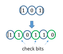
Код Хэмминга
Код Хэмминга — наиболее известный из первых самоконтролирующихся и самокорректирующихся кодов. Позволяет устранить одну ошибку и находить двойную.

Код Хэмминга (7,4) — 4 бита на входе кодера и 7 на выходе, следовательно 3 проверочных бита. С 1 по 4 информационные биты, с 6 по 7 проверочные (см. табл. выше). Пятый проверочный бит y5, это сумма по модулю два 1-3 информационных бит. Сумма по модулю 2 это вычисление бита чётности.
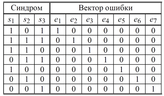
Декодирование кода Хэмминга
Декодирование происходит через вычисление синдрома по выражениям:
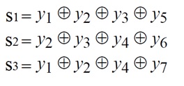
Синдром это сложение бит по модулю два. Если синдром не нулевой, то исправление ошибки происходит по таблице декодирования:
Расстояние Хэмминга
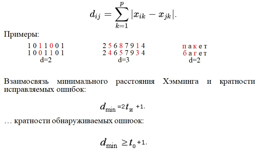
Расстояние Хэмминга — число позиций, в которых соответствующие символы двух кодовых слов одинаковой длины различны. Если рассматривать два кодовых слова, (пример на картинке ниже, 1 0 1 1 0 0 1 и 1 0 0 1 1 0 1) видно что они отличаются друг от друга на два символа, соответственно расстояние Хэмминга равно 2.
Кратность исправляемых ошибок и обнаруживаемых, связано минимальным расстоянием Хэмминга. Любой помехоустойчивый код добавляет избыточность с целью увеличить минимальное расстояние Хэмминга. Именно минимальное расстояние Хэмминга определяет помехоустойчивость.
Помехоустойчивые коды
Современные коды более эффективны по сравнению с рассматриваемыми примерами. В таблице ниже приведены Коды Боуза-Чоудхури-Хоквингема (БЧХ)
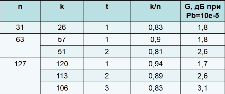
Из таблицы видим, что там один класс кода БЧХ, но разные параметры n и k.
- n — количество символов на входе.
- k — количество символов на выходе.
- t — кратность исправляемых ошибок.
- Отношение k/n — скорость кода.
- G (энергетический выигрыш) — величина, показывающая на сколько можно уменьшить отношение сигнал/шум (Eb/No) для обеспечения заданной вероятности ошибки.
Несмотря на то, что скорость кода близка, количество исправляемых ошибок может быть разное. Количество исправляемых ошибок зависит от той избыточности, которую добавим и от размера блока. Чем больше блок, тем больше ошибок он исправляет, даже при той же самой избыточности.
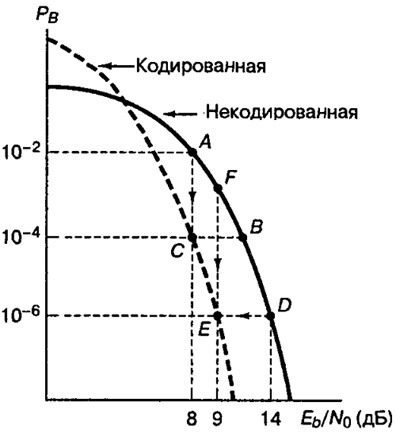
Пример: помехоустойчивые коды и двоичная фазовая манипуляция (2-ФМн). На графике зависимость отношения сигнал шум (Eb/No) от вероятности ошибки. За счет применения помехоустойчивых кодов улучшается помехоустойчивость.
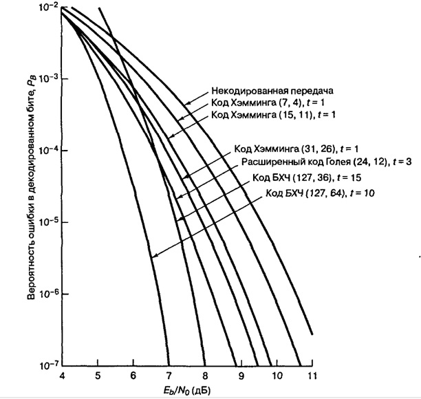
Из графика видим, код Хэмминга (7,4) на сколько увеличилась помехоустойчивость? Всего на пол Дб это мало, если применить код БЧХ (127, 64) выиграем порядка 4 дБ, это хороший показатель.
Компромиссы при использовании помехоустойчивых кодов
Чем расплачиваемся за помехоустойчивые коды? Добавили избыточность, соответственно эту избыточность тоже нужно передавать. Нужно: увеличивать пропускную способность канала связи, либо увеличивать длительность передачи.
Компромисс:
- Достоверность vs полоса пропускания.
- Мощность vs полоса пропускания.
- Скорость передачи данных vs полоса пропускания
Необходимость чередования (перемежения)
Все помехоустойчивые коды могут исправлять только ограниченное количество ошибок t. Однако в реальных системах связи часто возникают ситуации сгруппированных ошибок, когда в течение непродолжительного времени количество ошибок превышает t.
Например, в канале связи шумов мало, все передается хорошо, ошибки возникают редко, но вдруг возникла импульсная помеха или замирания, которые повредили на некоторое время процесс передачи, и потерялся большой кусок информации. В среднем на блок приходится одна, две ошибки, а в нашем примере потерялся целый блок, включая информационные и проверочные биты. Сможет ли помехоустойчивый код исправить такую ошибку? Эта проблема решаема за счет перемежения.
Пример блочного перемежения:

На картинке, всего 5 блоков (с 1 по 25). Код работает исправляя ошибки в рамках одного блока (если в одном блоке 1 ошибка, код его исправит, а если две то нет). В канал связи отдается информация не последовательно, а в перемешку. На выходе кодера сформировались 5 блоков и эти 5 блоков будем отдавать не по очереди а в перемешку. Записали всё по строкам, но считывать будем, чтобы отправлять в канал связи, по столбцам. Информация в блоках перемешалась. В канале связи возникла ошибка и мы потеряли большой кусок. В процессе приема, мы опять составляем таблицу, записываем по столбцам, но считываем по строкам. За счет того, что мы перемешали большое количество блоков между собой, групповая ошибка равномерно распределится по блокам.