Excel for Microsoft 365 Excel for Microsoft 365 for Mac Excel for the web Excel 2021 Excel 2021 for Mac Excel 2019 Excel 2019 for Mac Excel 2016 Excel 2016 for Mac Excel 2013 Excel 2010 Excel 2007 Excel for Mac 2011 Excel for Windows Phone 10 More…Less
This topic describes the most common VLOOKUP reasons for an erroneous result on the function, and provides suggestions for using INDEX and MATCH instead.
Tip: Also, refer to the Quick Reference Card: VLOOKUP troubleshooting tips which presents the common reasons for #NA issues in a convenient PDF file. You can share the PDF with others or print for your own reference.
Problem: The lookup value is not in the first column in the table_array argument
One constraint of VLOOKUP is that it can only look for values on the left-most column in the table array. If your lookup value is not in the first column of the array, you will see the #N/A error.
In the following table, we want to retrieve the number of units sold for Kale.

The #N/A error results because the lookup value “Kale” appears in the second column (Produce) of the table_array argument A2:C10. In this case, Excel is looking for it in column A, not column B.
Solution: You can try to fix this by adjusting your VLOOKUP to reference the correct column. If that’s not possible, then try moving your columns. That may also be highly impracticable, if you have large or complex spreadsheets where cell values are results of other calculations—or maybe there are other logical reasons why you simply cannot move the columns around. The solution is to use a combination of INDEX and MATCH functions, which can look up a value in a column regardless of its location position in the lookup table. See the next section.
Consider using INDEX/MATCH instead
INDEX and MATCH are good options for many cases in which VLOOKUP does not meet your needs. The key advantage of INDEX/MATCH is that you can look up a value in a column in any location in the lookup table. INDEX returns a value from a specified table/range—according to its position. MATCH returns the relative position of a value in a table/range. Use INDEX and MATCH together in a formula to look up a value in a table/array by specifying the relative position of the value in the table/array.
There are several benefits of using INDEX/MATCH instead of VLOOKUP:
-
With INDEX and MATCH, the return value need not be in the same column as the lookup column. This is different from VLOOKUP, in which the return value has to be in the specified range. How does this matter? With VLOOKUP, you have to know the column number that contains the return value. While this may not seem challenging, it can be cumbersome when you have a large table and have to count the number of columns. Also, if you add/remove a column in your table, you have to recount and update the col_index_num argument. With INDEX and MATCH, no counting is required as the lookup column is different from the column that has the return value.
-
With INDEX and MATCH, you can specify either a row or a column in an array—or specify both. This means you can look up values both vertically and horizontally.
-
INDEX and MATCH can be used to look up values in any column. Unlike VLOOKUP—in which you can only look up to a value in the first column in a table—INDEX and MATCH will work if your lookup value is in the first column, the last, or anywhere in between.
-
INDEX and MATCH offer the flexibility of making dynamic reference to the column which contains the return value. This means that you can add columns to your table without breaking INDEX and MATCH. On the other hand, VLOOKUP breaks if you need to add a column to the table—since it makes a static reference to the table.
-
INDEX and MATCH offers more flexibility with matches. INDEX and MATCH can find an exact match, or a value that is greater or lesser than the lookup value. VLOOKUP will only look for a closest match to a value (by default) or an exact value. VLOOKUP also assumes by default that the first column in the table array is sorted alphabetically, and suppose your table is not set up that way, VLOOKUP will return the first closest match in the table, which may not be the data you are looking for.
Syntax
To build syntax for INDEX/MATCH, you need to use the array/reference argument from the INDEX function and nest the MATCH syntax inside of it. This take the form:
=INDEX(array or reference, MATCH(lookup_value,lookup_array,[match_type])
Let’s use INDEX/MATCH to replace VLOOKUP from the example above. The syntax will look like this:
=INDEX(C2:C10,MATCH(B13,B2:B10,0))
In simple English it means:
=INDEX(return a value from C2:C10, that will MATCH(Kale, which is somewhere in the B2:B10 array, in which the return value is the first value corresponding to Kale))
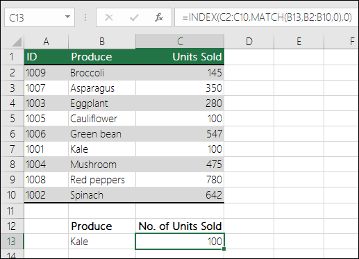
The formula looks for the first value in C2:C10 that corresponds to Kale (in B7) and returns the value in C7 (100), which is the first value that matches Kale.
Problem: The exact match is not found
When the range_lookup argument is FALSE—and VLOOKUP is unable to find an exact match in your data—it returns the #N/A error.
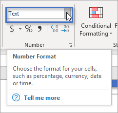
Solution: If you are sure the relevant data exists in your spreadsheet and VLOOKUP is not catching it, take time to verify that the referenced cells don’t have hidden spaces or non-printing characters. Also, ensure that the cells follow the correct data type. For example, cells with numbers should be formatted as Number, and not Text.
Also, consider using either the CLEAN or TRIM function to clean up data in cells.
Problem: The lookup value is smaller than the smallest value in the array
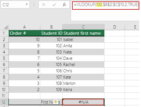
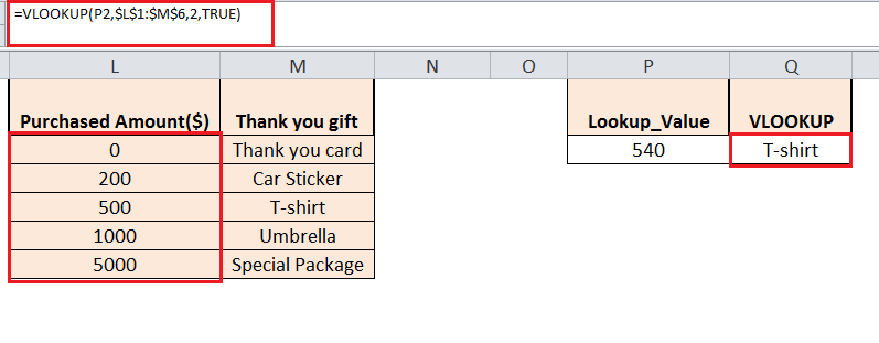
If the range_lookup argument is set to TRUE—and the lookup value is smaller than the smallest value in the array—you will see the #N/A error. TRUE looks for an approximate match in the array and returns the closest value lesser than the lookup value.
In the following example, the lookup value is 100, but there are no values in the B2:C10 range that are lesser than 100; hence the error.
Solution:
-
Correct the lookup value as necessary.
-
If you cannot change the lookup value and need greater flexibility with matching values, consider using INDEX/MATCH instead of VLOOKUP—see the section above in this article. With INDEX/MATCH, you can look up values greater than, lesser to, or equal to the lookup value. For more information on using INDEX/MATCH instead of VLOOKUP, refer to the previous section in this topic.
Problem: The lookup column is not sorted in the ascending order
If the range_lookup argument is set to TRUE—and one of your lookup columns is not sorted in the ascending (A-Z) order—you will see the #N/A error.
Solution:
-
Change the VLOOKUP function to look for an exact match. To do that, set the range_lookup argument to FALSE. No sorting is necessary for FALSE.
-
Use the INDEX/MATCH function to look up a value in an unsorted table.
Problem: The value is a large floating point number
If you have time values or large decimal numbers in cells, Excel returns the #N/A error because of floating point precision. Floating point numbers are numbers that follow after a decimal point. (Excel stores time values as floating point numbers.) Excel cannot store numbers with very large floating points, so for the function to work correctly, the floating point numbers will need to be rounded to 5 decimal places.
Solution: Shorten the numbers by rounding them up to five decimal places with the ROUND function.
Need more help?
You can always ask an expert in the Excel Tech Community or get support in the Answers community.
See Also
-
Correct a #N/A error
-
VLOOKUP: No more #NA
-
Floating-point arithmetic may give inaccurate results in Excel
-
Quick Reference Card: VLOOKUP refresher
-
VLOOKUP function
-
Overview of formulas in Excel
-
How to avoid broken formulas
-
Detect errors in formulas
-
All Excel functions (alphabetical)
-
All Excel functions (by category)
Need more help?
-
04-14-2005, 12:06 PM
#1
Value Not Available Error in Vlookup
I’m using the vlookup function to get a number back from a table. I’ve
created the vlookup properly but keep getting the #N/A with the message —
«Value Not Available Error». The problem is that the value is available.
I’ve copied the vlookup formula into a number of cells — all come back #N/A.
The puzzle is, I can get the formula to work if I retype the value being
looked up in the table. I’ve compared formats; I’ve made sure the table is
in alphabetical order; I can’t see any difference from the value being looked
up with the value in the table — they are even the same font.
Any ideas? The table is copied into the worksheet from another workbook.
Thanks for any help.
-
04-14-2005, 01:06 PM
#2
Re: Value Not Available Error in Vlookup
Hi
when you retype the value being lookup it tends to suggest a problem along
the lines of:
— calculation set to manual — tools / options / calculation -check that it
is set to automatic
— leading or trailing spaces in this value in the lookup value — type in
another cell =LEN(A1) where A1 is the cell reference of your lookup value to
find out how many characters excel sees the cell as having as compared to
how many you think it has
— numbers that aren’t really numbers if you’re looking up numbers — type in
another cell =ISNUMBER(A1) to test that what you think is a number is
acutally a number
-omitting the 4th parameter (0 or FALSE) for an exact match — although this
would normally raise wrong answers rather than an #NA errorhope this helps
—
Cheers
JulieD
check out www.hcts.net.au/tipsandtricks.htm
….well i’m working on it anyway
«thefeokas» <thefeokas@discussions.microsoft.com> wrote in message
news:65416377-E39F-4150-A189-DBDCEA3F49CF@microsoft.com…
> I’m using the vlookup function to get a number back from a table. I’ve
> created the vlookup properly but keep getting the #N/A with the message —
> «Value Not Available Error». The problem is that the value is available.
> I’ve copied the vlookup formula into a number of cells — all come back
> #N/A.
> The puzzle is, I can get the formula to work if I retype the value being
> looked up in the table. I’ve compared formats; I’ve made sure the table
> is
> in alphabetical order; I can’t see any difference from the value being
> looked
> up with the value in the table — they are even the same font.
> Any ideas? The table is copied into the worksheet from another workbook.
> Thanks for any help.
-
04-14-2005, 01:06 PM
#3
Re: Value Not Available Error in Vlookup
That did it! I found that there were spaces in the lookup table at the end of
the values. I used Replace… to remove the trailing spaces.
Thanks.«JulieD» wrote:
> Hi
>
> when you retype the value being lookup it tends to suggest a problem along
> the lines of:
> — calculation set to manual — tools / options / calculation -check that it
> is set to automatic
> — leading or trailing spaces in this value in the lookup value — type in
> another cell =LEN(A1) where A1 is the cell reference of your lookup value to
> find out how many characters excel sees the cell as having as compared to
> how many you think it has
> — numbers that aren’t really numbers if you’re looking up numbers — type in
> another cell =ISNUMBER(A1) to test that what you think is a number is
> acutally a number
> -omitting the 4th parameter (0 or FALSE) for an exact match — although this
> would normally raise wrong answers rather than an #NA error
>
> hope this helps
> —
> Cheers
> JulieD
> check out www.hcts.net.au/tipsandtricks.htm
> ….well i’m working on it anyway
> «thefeokas» <thefeokas@discussions.microsoft.com> wrote in message
> news:65416377-E39F-4150-A189-DBDCEA3F49CF@microsoft.com…
> > I’m using the vlookup function to get a number back from a table. I’ve
> > created the vlookup properly but keep getting the #N/A with the message —
> > «Value Not Available Error». The problem is that the value is available.
> > I’ve copied the vlookup formula into a number of cells — all come back
> > #N/A.
> > The puzzle is, I can get the formula to work if I retype the value being
> > looked up in the table. I’ve compared formats; I’ve made sure the table
> > is
> > in alphabetical order; I can’t see any difference from the value being
> > looked
> > up with the value in the table — they are even the same font.
> > Any ideas? The table is copied into the worksheet from another workbook.
> > Thanks for any help.
>
>
>
-
04-14-2005, 01:06 PM
#4
Re: Value Not Available Error in Vlookup
you’re welcome and thanks for the feedback
—
Cheers
JulieD
check out www.hcts.net.au/tipsandtricks.htm
….well i’m working on it anyway
«thefeokas» <thefeokas@discussions.microsoft.com> wrote in message
news:62E30085-F56C-42F5-8C8C-D1DAABED6CF2@microsoft.com…
> That did it! I found that there were spaces in the lookup table at the end
> of
> the values. I used Replace… to remove the trailing spaces.
> Thanks.
>
> «JulieD» wrote:
>
>> Hi
>>
>> when you retype the value being lookup it tends to suggest a problem
>> along
>> the lines of:
>> — calculation set to manual — tools / options / calculation -check that
>> it
>> is set to automatic
>> — leading or trailing spaces in this value in the lookup value — type in
>> another cell =LEN(A1) where A1 is the cell reference of your lookup value
>> to
>> find out how many characters excel sees the cell as having as compared to
>> how many you think it has
>> — numbers that aren’t really numbers if you’re looking up numbers — type
>> in
>> another cell =ISNUMBER(A1) to test that what you think is a number is
>> acutally a number
>> -omitting the 4th parameter (0 or FALSE) for an exact match — although
>> this
>> would normally raise wrong answers rather than an #NA error
>>
>> hope this helps
>> —
>> Cheers
>> JulieD
>> check out www.hcts.net.au/tipsandtricks.htm
>> ….well i’m working on it anyway
>> «thefeokas» <thefeokas@discussions.microsoft.com> wrote in message
>> news:65416377-E39F-4150-A189-DBDCEA3F49CF@microsoft.com…
>> > I’m using the vlookup function to get a number back from a table. I’ve
>> > created the vlookup properly but keep getting the #N/A with the
>> > message —
>> > «Value Not Available Error». The problem is that the value is
>> > available.
>> > I’ve copied the vlookup formula into a number of cells — all come back
>> > #N/A.
>> > The puzzle is, I can get the formula to work if I retype the value
>> > being
>> > looked up in the table. I’ve compared formats; I’ve made sure the
>> > table
>> > is
>> > in alphabetical order; I can’t see any difference from the value being
>> > looked
>> > up with the value in the table — they are even the same font.
>> > Any ideas? The table is copied into the worksheet from another
>> > workbook.
>> > Thanks for any help.
>>
>>
>>
VLOOKUP is very common, popular and widely used function in Excel and Google Sheets. But the majority of users complain that VLOOKUP is not working correctly or giving incorrect results. This is because of some limitations with the VLOOKUP function, and sometimes users also do not carefully follow its rules and syntax. Here, we are going to discuss some of the common errors and reasons why VLOOKUP does not work.
Common VLOOKUP Errors
In this article, we are going to discuss VLOOKUP errors, like #NA, #VALUE, #REF, and VLOOKUP returning incorrect results. Now you are going to see the reasons for these errors and their solutions.
VLOOKUP #NA error
When VLOOKUP formula cannot find a match, then this error displays, meaning “not available.” But it is always not correct that the lookup value is actually not available. There could be some reasons why VLOOKUP returns this error.
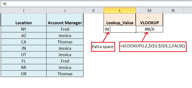
- Extra Spaces in Lookup Value. This is one of the most common reasons behind the #NA error in VLOOKUP. In big data set it is very hard to identify these leading or trailing spaces in lookup values that cause the VLOOKUP function to not find the match and return #NA error.

Solution:
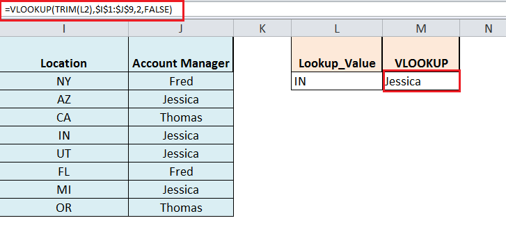
To kill these extra spaces, you need to wrap the Lookup_value argument in the VLOOKUP formula with the TRIM function to ensure correct working of the function, such as;
=VLOOKUP(TRIM(L2),$I$1:$J$9,2,FALSE) - Typo mistake in Lookup_Value. If you wrongly enter the value in the lookup_value argument of VLOOKUP function, then it generates the #NA error. So you must enter the lookup value correctly in the lookup_value argument.
- Numeric values are formatted as Text. If numeric values are formatted as text in a table_array argument of VLOOKUP function, then it comes up with the #NA error.
To fix this error, you must check and properly format the numeric values as “Number.”
- Lookup Value not in First column of table array. As per rule lookup value must be in the first (leftmost) column of a table_array argument of the VLOOKUP function. If lookup value is not present in the first column of a table_array, then VLOOKUP generates #NA error.
To fix this error, you must arrange your columns correctly and then select your table_array in VLOOKUP function.
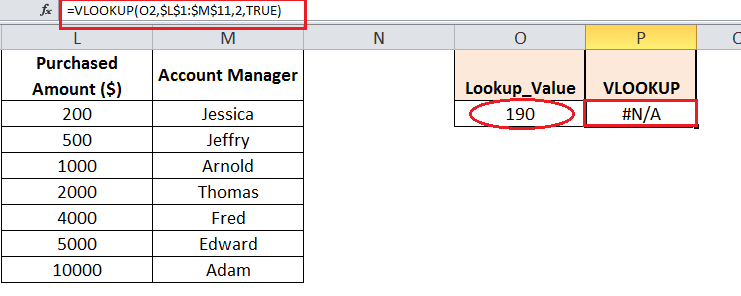
- In case of Approximate Match typeIn case of approximate match type (TRUE), your VLOOKUP function generates #NA error if your lookup value is smaller than the smallest value available in the first column of table_array.

VLOOKUP #VALUE error
Generally, if you enter wrong data type in the formula in Excel, then formula generates #Value error. But in the case of VLOOKUP function, there are following three reasons that should look into.
- Index_number less than 1. If you enter index_number argument less than 1 in VLOOKUP function, then it returns a #VALUE error. So you must check index_number argument if VLOOKUP argument returns this error.
- Workbook path is incorrect or incomplete: When you supply the table_array from another workbook in VLOOKUP and path of that workbook is incomplete then VLOOKUP returns a #VALUE error. So you need to follow its following syntax to provide it fully.
=VLOOKUP(lookup_value, '[workbook name]sheet name'!table_array, col_index_num, FALSE)If anything in the path format is missing, VLOOKUP formula returns a #VALUE error, unless the lookup workbook is currently open.
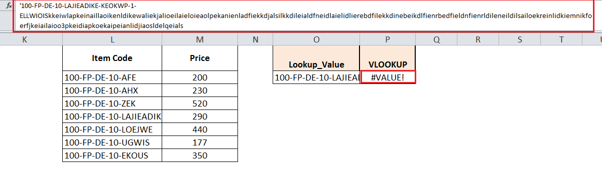
- Lookup value characters length. VLOOKUP supports a maximum of 255 characters length of a lookup value argument. If lookup value character length exceeds this limit in VLOOKUP, then formula returns a #VALUE error.
Solution:
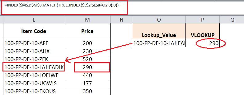
Either you can reduce the character length of the lookup value to the maximum limit of 255 characters in the VLOOKUP function or you should use INDEX, MATCH formula instead of the VLOOKUP function in the following pattern;
=INDEX (returing_range,MATCH(TRUE,INDEX(lookup_range = lookup_value,0),0))=INDEX($M$2:$M$8,MATCH(TRUE,INDEX($L$2:$L$8=O2,0),0))
VLOOKUP #REF error
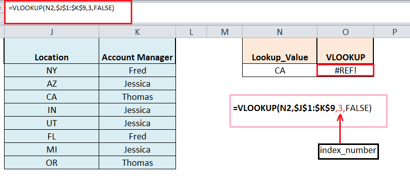
If the index_number argument of VLOOKUP is greater than the number of columns in table_array, then the VLOOKUP function returns a #REF error. So you need to check and rectify the index_number supplied in function.
VLOOKUP returning incorrect results
If you omit to supply match type in a range_lookup argument of VLOOKUP then by default it searches for approximate match values, if it does not find exact match value. And if table_array is not sorted in ascending order by the first column, then VLOOKUP returns incorrect results.
Solution:
You must always supply a relevant match type in a range_lookup argument of VLOOKUP as TRUE or FALSE. And in case of approximate match type (TRUE), you must always sort your table_array in ascending order by the first column of your table_array.
Still need some help with Excel formatting or have other questions about Excel? Connect with a live Excel expert here for some 1 on 1 help. Your first session is always free.
Are you still looking for help with the VLOOKUP function? View our comprehensive round-up of VLOOKUP function tutorials here.
Bottom Line: Get explanations for common formula errors that are returned by lookup functions like VLOOKUP or INDEX MATCH.
Skill Level: Beginner
Download the Excel File
Follow along with me in the video, using the same Excel file I use. You can download it here:
Handling Formula Errors in Excel
VLOOKUP formulas can return a lot of errors, which can be both frustrating and time consuming. In this post, I’d like to show you some of the most common VlOOKUP and INDEX MATCH errors and how to deal with them.
Formula errors are typically caused by an issue within the argument(s) of the function. Formula errors always start with the pound/hashtag symbol (#).
You’ll notice that any cell which contains a formula error has a little green triangle in the upper left corner. In addition, there is an error button that appears next to the cell. When you click on it, you’ll get a menu that gives a bit more information about the error, including the error name.
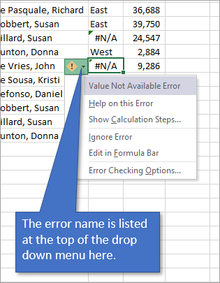
#N/A Error
The #N/A Error stands for Value Not Available. This is the most common error and it simply means that when Excel searches the specified range for a certain value, it doesn’t find that value. Sometimes, that’s exactly the information you need to know, but occasionally, this error is caused because of a slight mismatch that can be caused by a misspelling, extra spaces that are hard to see, or the data type of the cell.
Let’s look at each of those reasons individually.
1. Typo
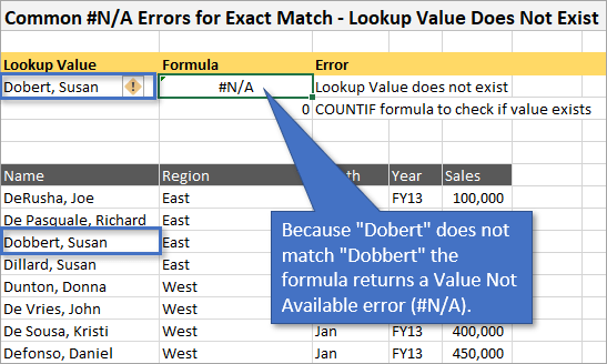
In this first example, VLOOKUP is looking to return a value for any time it finds the entry “Dobert, Susan”. But the problem is that we’ve misspelled the last name Dobbert, leaving out the second b. Since VLOOKUP cannot find the entry exactly as we’ve typed it, it returns a Value Not Available error.
The way to fix this is of course to correct the typo. Once the values match because you’ve fixed the error, the formula will return the correct answer that it is looking for.
Keep in mind that if the purpose of your VLOOKUP formula is not to return a value from another column, but to simply see if the value you are looking for exists, an alternative formula you can use is COUNTIF. That formula returns the number of times it finds the specified value in the range you’ve designated. (In other words, if there are three instances of the value you’re looking for, the formula will return the number 3. If there aren’t any instances of that value, you will get a 0.)
2. Number Stored as Text
The data type of your cells can also cause a mismatch between what VLOOKUP is looking for and what actually exists. So even though the values look the same (in the case below, the number we are looking for, 10001, is in our list), the problem is that Excel sees one cell as a number and the other cell as text.
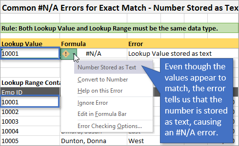
To correct the issue, you can change the data type. This can be done by choosing the second option in the menu, Convert to Number. Or it can also be done by changing the format in the Number section on the Home tab of the Ribbon.
3. Trailing Spaces
Sometimes, entries appear to match, but Excel doesn’t recognize them as an exact match because one of the entries has some additional spaces trailing at the end of the value.
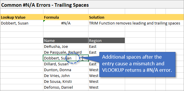
To fix the mismatch, you can manually remove the trailing spaces from the entries that have them. Or, another option is to use the TRIM function to remove any leading or trailing spaces from a range of data. Once you’ve trimmed them, you can either overwrite your old range with the newly trimmed range, or you can expand your VLOOKUP columns to include the newly trimmed cells.
Although #N/A is the most common error you will encounter when using VLOOKUP, there are some others as well. Three other errors that we can take a look at are #REF, #VALUE, and #NAME.
1. #REF Error
This error happens most often when columns get deleted from a sheet and that messes with the formula parameters. Usually it’s an indicator that the column index is outside the lookup range. For example, the column index is set to 3, but because you deleted a column, there are only two columns left in the range.
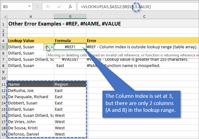
To fix the error, simply correct the column index number.
2. #VALUE Error
One reason you’ll see a #VALUE error can be when you have a 0 in the column index. This sometimes happens when you use 1 and 0 instead of TRUE and FALSE at the end of your argument. To fix the problem, just correct the column index like we did for the #REF error example above.
Another reason you’ll see a #VALUE error is when the lookup value contains more than 255 characters. Obviously, this is not typically something you would see, and there’s really no way to correct it besides reducing the number of characters in your data, if possible.
Just a side tip: Any time you want to know how many characters are in a cell you can use the LENGTH function. Simply type =LEN and then the name of the cell in question.
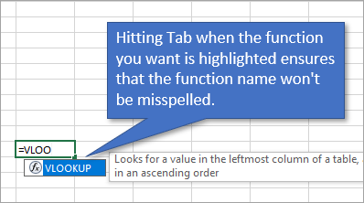
3. #NAME Error
The #NAME error occurs when you’ve misspelled the function name. To correct this error, just fix the spelling mistake.
You can avoid spelling errors in function names by pressing the Tab key when you start to type out the name of the function and see the one you want highlighted in the menu below your typing.
Using the IFERROR Function to Handle Formula Errors
Sometimes, the error being returned is a legitimate answer to our lookup, such as when there really isn’t a lookup value in the data source, and that’s just what we want to know. However, the #N/A error looks ugly on the spreadsheet.
We can return a different value for the formula error. To change the outcome so that it is blank or returns a word/phrase of our choosing, we can use the IFERROR function. The IFERROR function is a simple argument that just returns an alternate value (or a blank cell) whenever an error is found.
To use the IFERROR function, simply wrap it around the VLOOKUP formula. For example,
=VLOOKUP(A4,$A$12:$C$19,2,FALSE)
would become
=IFERROR(VLOOKUP(A4,$A$12:$C$19,2,FALSE),”ERROR”)
to return the word “ERROR” if an error is found. Of course you could make that word anything you want it to be. If you prefer that a blank cell be returned, just put nothing between the two quotation marks.
Don’t Use the IFERROR Unilaterally
You might have the idea to just always wrap your lookup functions in the IFERROR function so that you don’t have to see ugly errors on your spreadsheet. But I don’t recommend that.
The reason is that, as we saw in several of the errors above, there is often an action that needs to be taken to fix the errors, such as correcting spelling or indexes. You definitely want to be notified of those opportunities to fix the lookup results instead of leave them as errors.
Overview of Common Lookup Errors
I’ve condensed all of the error reasons that we’ve discussed in this post into the following image. It can also be found in the practice Excel file at the top of this post or you can download the printable PDF if you prefer.
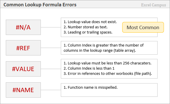
I hope this helps you to identify and fix the errors that you encounter when using lookup. Please let me know if you have any questions in the comments!
There are different reasons due to which error values are shown in active worksheet in Excel. The #N/A error values is one of them. There are few important reason due to which VLookup #N/A error shown in Excel sheet.
Excel display different kind of Excel error values like #DIV/0, #N/A, #NAME?, #NULL!, #NUM!, #REF! and #VALUE!. There are different specific reasons due to which these error values in Excel are generated. You can take some precautions or edit the formula so that you can easily resolve the issue of these errors in Excel.
#N/A error value mans that there is no value available. Normally this is not an error value but it is a special type of value. This kind of error values generated when given formula can’t able to find what it’s been asked to lookup. Normally #N/A error values generated with VLookup, HLookup, Lookup and Match functions when given formula not able to find the given referenced value. There are two common reasons due to which VLookup #N/A error show in Excel sheet, let’s start the discussion.
- How to create What IF Analysis data table in MS Excel
- How to Identifying Duplicate Values in two Excel worksheets
First Common reason why #N/A happens with VLookup in Excel
During working in any worksheet, sometime you will get #N/A error value when you are using VLookup function in active worksheet. The reason behind this error values is that after applying the VLookup formula in one cell when you drag the formula down to rest of the cells the table is not correctly referenced. In that situation #N/A error values generated in active worksheet.
If you want to resolve this kind of error value this you must have to check and update the reference type into Absolute reference to solve the issue. All we know there are 3 type reference type which is used in Excel formula- Relative, Absolute & Mixed. Normally Relative reference is used in different formulas but if you try to copy or drag the formula to rest of the cells generate the error values.

Step 1: Create the following given table in your active worksheet.
Step 2: Type the following VLookup function in cell C3 =VLOOKUP(B3,F3:G11,2,0) and drag this formula for rest of the cells C3:C14. Now when you drag this formula you can check there are few item names shown #N/A error value in C column.
Step 3: If you want to resolve this type of error then press F2 on cell C3 or you can also double click on Cell C3 to edit the formula.
Step 4: Change the range reference type from relative to absolute like this =VLOOKUP(B3,$F$3:$G$11,2,0) and drag this formula to rest of the cells. To change the reference type you can use F4 shortcut key or you can also do this job by manually typing the dollar ($) sign.
- How to Search Duplicate Values with VLookup function
- Combine IF with VLookup Function to hide any errors message
Second Common reason why #N/A happens with VLookup in Excel
If you already change the reference type of given formula but #N/A error values is still show in active worksheet. In that situation you have to check both Lookup and reference value. If both values doesn’t match then you have to check and correct the spelling mistake or remove any extra spaces.

Step 1: Create the following given table in your active worksheet.
Step 2: Type the following VLookup function in cell C3 =VLOOKUP(B3,$F$3:$G$11,2,0) and drag this formula for rest of the cells C3:C14. Now when you drag this formula you can check there are few item names shown #N/A error value in C column.
Step 3: Remove the extra single space from cell F3 and also correct the spelling mistake in Cell F7. Now, you can check #N/A error value has been removed and you will get final resulted value in the respective cells.
I hope after reading this guide you can easily understand what is the exact reasons why VLookup #N/A error shown in Excel sheet. If you have any suggestion regarding this guide then please write us in the comment box. Thanks to all.
Top 4 Errors in VLOOKUP and How to Fix Them?
The VLOOKUP function cannot give you errors due to data mismatch. Instead, it may return the errors.
- #N/A Error
- #NAME? Error
- #REF! Error
- #VALUE! Error
Let us discuss each error in detail with an example.
Table of contents
- Top 4 Errors in VLOOKUP and How to Fix Them?
- #1 Fixing #N/A Error in VLOOKUP
- #2 Fixing #VALUE! Error in VLOOKUP
- #3 Fixing VLOOKUP #REF Error
- #4 Fixing VLOOKUP #NAME Error
- Things to Remember Here
- Recommended Articles
You can download this Fix Errors in VLOOKUP Excel template here – Fix Errors in VLOOKUP Excel template
#1 Fixing #N/A Error in VLOOKUP
This error usually comes due to one of the many reasons. For example, the #N/A error means “Not Available.” It is the result of the VLOOKUP formula if the formula cannot find the required value.
Before fixing this problem, we need to know why it is giving an error as #N/A. This error is due to data entry mistakes, approximate match criteria, wrong table references, wrong column reference number, data not in vertical form, etc.
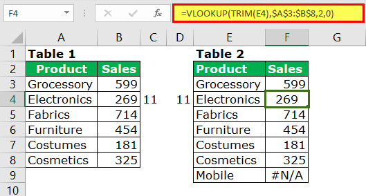
We have a sales report table in Table 1. In Table 2, we have applied the VLOOKUP formulaThe VLOOKUP excel function searches for a particular value and returns a corresponding match based on a unique identifier. A unique identifier is uniquely associated with all the records of the database. For instance, employee ID, student roll number, customer contact number, seller email address, etc., are unique identifiers.
read more and tried to extract the values from Table 1.

In cells F4 and F9, we got errors as #N/A.That is because cell E4 looks exactly the value in cell A4. But still, we got an error a #N/A. You must be thinking why VLOOKUP has returned the result as #N/A. Nothing to worry about. Follow the below steps to rectify the error.
- Step 1: We must apply the LEN excelThe Len function returns the length of a given string. It calculates the number of characters in a given string as input. It is a text function in Excel as well as an inbuilt function that can be accessed by typing =LEN( and entering a string as input.read more formula and find how many characters are in cells A4 and E4.
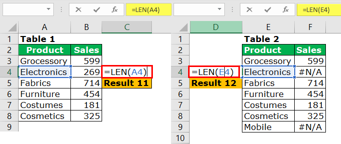
In cell C4, we have applied the LEN function to check how many characters are in cell A4. Similarly, we have used the LEN function in cell D4 to find how many characters are in cell E4.
In the A4 cell, we have 11 characters. But in cell E4, we have 12 characters. So one extra character is in cell E4 compared to cell A4.
By looking at the outset, both look similar to each other. However, there is one extra character. It must be a trailing space.
We can edit cell E4 and delete the space. If we delete this extra space, we will get the result.
But that is not the appropriate way to solve the issue.
- Step – 2: We can remove trailing spaces using the TRIM function in excelThe Trim function in Excel does exactly what its name implies: it trims some part of any string. The function of this formula is to remove any space in a given string. It does not remove a single space between two words, but it does remove any other unwanted spaces.read more. We can automatically delete the spaces by applying the VLOOKUP function and the TRIM function.
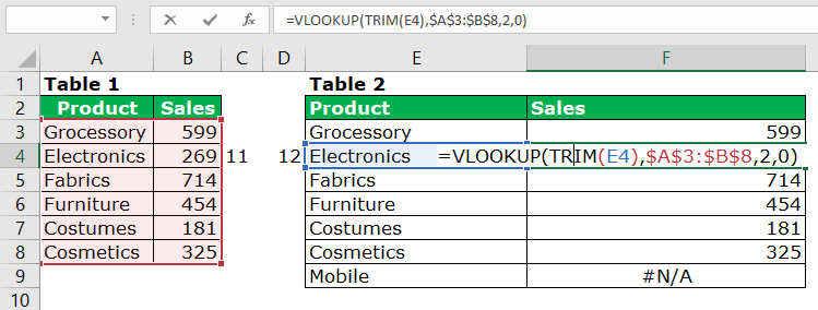
The TRIM function removes the extra unwanted space.
#2 Fixing #VALUE! Error in VLOOKUP
This error is due to missing any of the parameters in the function. For example, let us look at the below table.
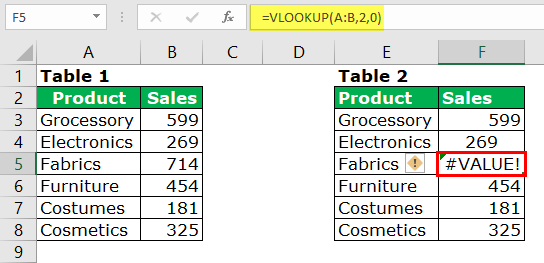
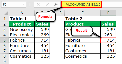
The VLOOKUP function starts with the LOOKUP value, the table range, column index number, and match type. If we look at the above image, the formula parameters are not in perfect order. In the place of the LOOKUP value, there is a table range. In the table range, we have column index numbers and so on.
We need to mention the formula correctly to remove this error.
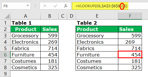
#3 Fixing VLOOKUP #REF Error
This error is due to the wrong reference number. When applying or mentioning the column index number, we must reveal the exact column number from which column we are looking at the required result. If we state the column index number out of the selection range, this will return #REF! Error.

The LOOKUP value is perfect. Also, the table range is excellent. But the column index number is not perfect here. Therefore, we selected the table range from A3 to B8, which means we have chosen only two columns.
In the column index number, we have mentioned 3, which is out of range of the table range, so the VLOOKUP returns the #REF! Error result.
We must mention the correct column index number to rectify this error.
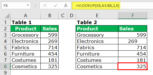
#4 Fixing VLOOKUP #NAME Error
The VLOOKUP #NAME? Error displays due to the mentioned wrong formula. In my personal experience, we usually type CLOOKUP instead of VLOOKUP.
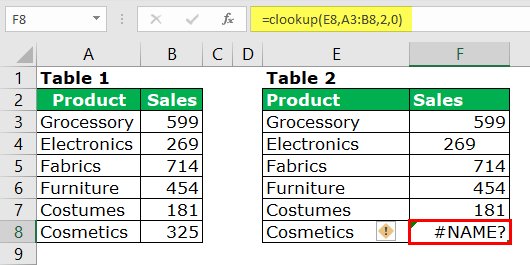
There is no formula called CLOOKUP in Excel, so returned the values as #NAME? Error type.
Solution: The solution is straightforward. We must check the formula’s spelling.
Things to Remember
- The #N/A error may occur due to data mismatch.
- The #NAME? Error may appear due to the wrong formula type.
- The #REF! Error may display due to a wrong column index number.
- The #VALUE! Error is due to a missing or incorrect parameter supply.
Recommended Articles
This article is a guide to the VLOOKUP Errors in Excel. We discuss fixing the four most common errors #N/A, #VALUE! #NAME? And REF! in the VLOOKUP function, Excel example, and downloadable Excel templates. You may also look at these useful functions in Excel: –
- Vlookup to Left
- VLookup with IF Function
- Multiple Criteria of VLOOKUP
- IFERROR with VLOOKUP in Excel
-
#1
I have a list that looks up a Grade letter for a GPA. I have 5 Classes, each class shows a grade (by letter) in one Cell and in another Cell I have a VLOOKUP that gets the GPA based on the Letter Grade. However, with the 5th VLOOKUP I get a Value of #N/A instead of the GPA, which I get returned for the other 4.
Here is the VLOOKUP formula’s:
=VLOOKUP(F6,B22:C32,2,TRUE)
=VLOOKUP(F7,B22:C32,2,TRUE)
=VLOOKUP(F8,B22:C32,2,TRUE)
=VLOOKUP(F9,B22:C32,2,TRUE)
=VLOOKUP(F10,B22:C32,2,TRUE)
The lookup field Goes to the following, Starting cell has the Value A-, end cell is 0:
Grade Credit
A- 3.7
A- 4
B- 2.7
B 3
B+ 3.3
C- 1.7
C 2
C+ 2.3
D 1
D+ 1.3
F 0
Here’s what the GPA cells have
Class Grade Percentage GPA
Class Grade Percentage GPA
Biology B 86.92 4
English C+ 79.71 2.3
Geometry B- 81.79 2.7
French D- 64.93 1
World History A- 95.38 #N/A
At first I thought it might be because of the negative, but it couldn’t be because there is a B- showing. So I changed the grade to Show an A and it still shows the #N/A. Any thoughts?
Using Function Arguments with nested formulas
If writing INDEX in Func. Arguments, type MATCH(. Use the mouse to click inside MATCH in the formula bar. Dialog switches to MATCH.
-
#2
Welcome to the board…
Try changing TRUE to FALSE
Hope that helps.
-
#3
Nope. Thanks though.
Not sure if it has anything to do with it being the last one in the list or not, I wouldn’t it is.
Also, I changed the sorting order a few different times and that did not help either.
::Update::
Odd… I just tried to see if it has anything to do with it being the last one and it doesn’t but I did just notice that if I change the Grade to anything other than an A it works fine. If I change it to a B it gives a GPA of 4. Odd…. very strange.
Last edited: May 25, 2011
-
#4
Well it’s working for me to an extent…
1. You have A- listed twice in B22 and B23
2. You do not have D- Listed.
| Excel Workbook | ||||
|---|---|---|---|---|
|
|
||||
| E | F | G | H | |
| 4 | Class | Grade | Percentage | GPA |
| 5 | Class | Grade | Percentage | GPA |
| 6 | Biology | B | 86.92 | 3 |
| 7 | English | C+ | 79.71 | 2.3 |
| 8 | Geometry | B- | 81.79 | 2.7 |
| 9 | French | D- | 64.93 | #N/A |
| 10 | World History | A- | 95.38 | 3.7 |
|
Sheet2 |
| Excel Workbook | ||
|---|---|---|
|
|
||
| B | C | |
| 22 | A- | 3.7 |
| 23 | A- | 4 |
| 24 | B- | 2.7 |
| 25 | B | 3 |
| 26 | B+ | 3.3 |
| 27 | C- | 1.7 |
| 28 | C | 2 |
| 29 | C+ | 2.3 |
| 30 | D | 1 |
| 31 | D+ | 1.3 |
| 32 | F | 0 |
|
Sheet2 |
-
#5
I re-created this in a spreadsheet and it works fine. I would recommend that you check your formula in cell H10 to make sure the VLOOKUP range is correct. Make sure it is looking to B22:C32
-
#6
I created the sheet again and still the same issue. even when I use False. I just cannot figure out why.
-
#7
You have A- twice. Is that correct?
-
#8
The #NA error usually refers to the item you’r looking up not being in the lookup table, try checking the spellings correct in the lookup value and the table and also check there’s no leading or trailing spaces.
-
#9
No, I no Longer have A- twice.
I have the following table I am looking at.
Code:
Grade	Credit
A  	4
A+	4.1
A- 	3.7
B	3
B+	3.3
B-  	2.7
C	2
C+	2.3
C- 	1.7
D  	1
D+	1.3
F 	0
Since I have updated the look up table as shown above, It works with A+ but not A or A-.
I’ve also checked for additional spaces and extra characters, so I do not believe that is the case.
:::UPDATE:::
Ok, I’ve gotten it fixed. Some how after I checked for Spacing, I went back and looked again and there was an additional space I didn’t catch or added somehow. So it is working now. Just keep in mind I did create the spreadsheet again to get it to work. I do not know why it didn’t work with the earlier version with the spaces removed. Possibly due to formatting or another issue.
Thanks again for your input and help.
Last edited: May 25, 2011
-
#10
Glad you got it sorted. It may well that the formatting carries extra spaces