Содержание
- A physics teacher
- Tuesday, December 22, 2009
- what is a parallax error?
- Parallax is great! Gaia will expand our view
- What is parallax?
- Why is parallax such a good method?
- How far can it reach? (Classical)
- The annoying nature of errors in parallax measurements: part I
- The annoying nature of errors in parallax measurements: part II
- How far can it reach? (Classical, again)
- How far can it reach? (Hipparcos)
- How far can it reach? (Gaia)
- Hipparcos vs. Gaia: The case of RR Lyr
- Hipparcos vs. Gaia: The general trend
- What about radio measurements?
- For more information
A physics teacher
Physics lesson online brought to you by a physics teacher.

Tuesday, December 22, 2009
what is a parallax error?
Parallax error is the error that is most committed when readings are taken in physics. You can thus understand why it is important to avoid it at all cost. One must be aware of its existence at all time so that it can be avoided and as a result the true value of the reading is obtained.
The concept of parallax error is related to the term parallax.
Imagine that we have in a room a pelican and a flamingo as shown in fig 1 below.
Now Garfield is moving about in the room and each time is is somewhere in the room, he looks at the two birds. At the point A he sees the flamingo on the left of the pelican whereas when he is at position C he would see the flamingo on the right of the pelican. Only when he would be at position B would he sees the two birds one behind the other.
He would discover that each time he is at a different position, he would find that the position of the flamingo relative to the pelican has changed.
You can also have this effect when you are in front of a clock. If you move from side to side you would find that the time that you can read from the clock is different.
So we can the understand that the parallax is the change in the apparent position of an object when the position of the observer changes.
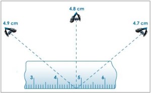
Now let us look at the concept of parallax error. If you have placed a pencil on a metre rule and you are reading its length then just like in fig 1 above and in fig 2 below you can place you eye everywhere you want.

As you can see from fig 2 above I have chosen three position at which you can place your eye.
Clearly at these three position we can have the following reading
Reading at A = 6.2 cm
Reading at B = 5.8 cm
Reading at C = 5.5 cm
What you you think would be the correct reading?
The correct reading is would be obtained when the eye is placed at B.

Now there is a line from the tip of eye to the of the pencil that continues up to the scale. this line is called the line of sight and the mark at which the line intersect the scale is the length of the pencil. This line of sight must be be at right angle to the scale. This is shown above in fig
If the line of sight and the scale are not ar right angle to each other then a parallax error is committed.
Similarly with a measuring cylinder the line of sight from the eye to the bottom of the meniscus must be at right angle to the scale as shown in fig 4 below. In this case the line of sight is horizontal and the scale vertical.

So as you can see above each time you are taking a reading you must ensure that the line of sight is perpendicular to the scale.
Источник
Parallax is great! Gaia will expand our view
What is parallax?
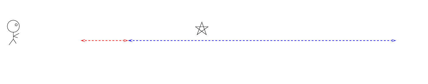
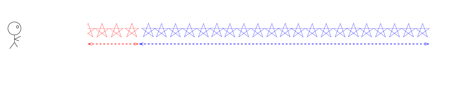
Parallax is the apparent shift in position of a nearby object when it is viewed from different locations. Those might be two different observatories on the Earth’s surface (as was the case in the famous transits of Venus in the eighteenth and nineteenth centuries), but, in most astronomical applications, are two spots in Earth’s orbit around the Sun:
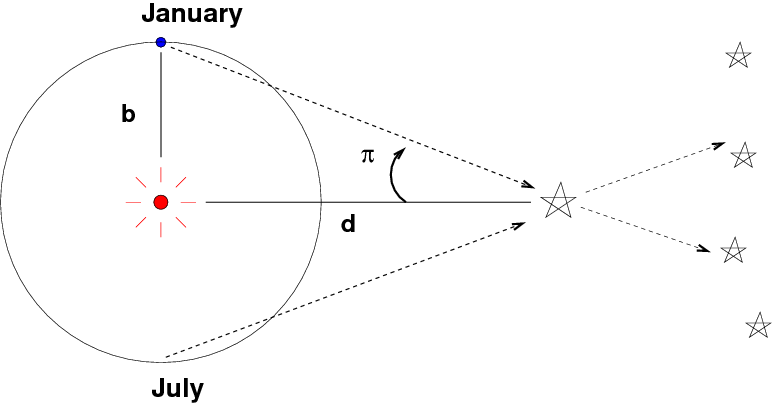
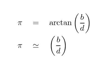
If one knows the value of the baseline distance b, and can measure the parallax angle π
Yes, I know this is confusing. Yes, astronomers back in the old days should have picked a better letter. Sometimes you see the «curly pi» used to denote this angle, but few font families include it
then one can use simple geometry to compute the distance to the target object d.
Of course, that simple formula ignores many complications. For example,
- the target object is usually located far above or below the plane of the Earth’s orbit
- the target star and the Sun are both moving through the Milky Way Galaxy
- the background reference stars are not located at an infinite distance, and so suffer their own small parallactic shifts
- the background stars aren’t even all at the same distance
But one can work around these issues, or at least place constraints on their consequences.
Why is parallax such a good method?
The importance of parallax lies in its fundamental simplicity: we humans understand geometry, and trust it. As long as we can make measurements of the angular displacements over time, we can use the resulting distances with confidence.
There may be minor issues involving corrections for the small shifts of the background reference stars themselves; but if we choose to use galaxies or quasars as the reference sources, we can avoid those completely.
Most important of all, parallax is a direct method of measuring distances. It relies on a single assumed quantity: the astronomical unit (AU) = the distance from Earth to Sun. Back in the 1800s and early 1900s, this was indeed a major issue, and astronomers great efforts to pin down the value of the AU. But these days, thanks to radar and spacecraft flying through the solar system, we do have a very, very good idea for the size of the AU. For example, the JPL Horizons system uses a value taken from the Planetary and Lunar Ephemerides DE430 and DE431, which list
That’s . quite a few signficant figures.
And that’s it. Heliocentric parallax does NOT require any assumptions about stellar luminosity or evolution, or the distribution of sizes and colors of stars, or the spectral energy distribution of glowing hydrogen gas.
So, if astronomers can measure a distance via parallax, they will rely on it much more than distances determined by other methods.
How far can it reach? (Classical)
So, parallax is a good method. But how far out into space can it reach?
Back in the old days, when parallax was performed by optical telescopes from the surface of the Earth, it was very difficult to achieve precisions of better than about 0.01 arcsec. Let’s use milliarcseconds (mas) from this point forward, as it will be more convenient. So, good ground-based measurements had precisions of perhaps 10 mas.
The very best, made with specially-built instruments such as the Multichannel Astrometric Photometer at Allegheny Observatory , could achieve precision of 1 mas for a few stars, after many observations.
However, no such devices could make all-sky surveys. As a result, catalogs of stellar distances were incomplete, as well as being rather low in precision. For example, the Bright Star Catalog , compiled over the period of 1964 to 1991, listed parallax values for about 2700 stars.
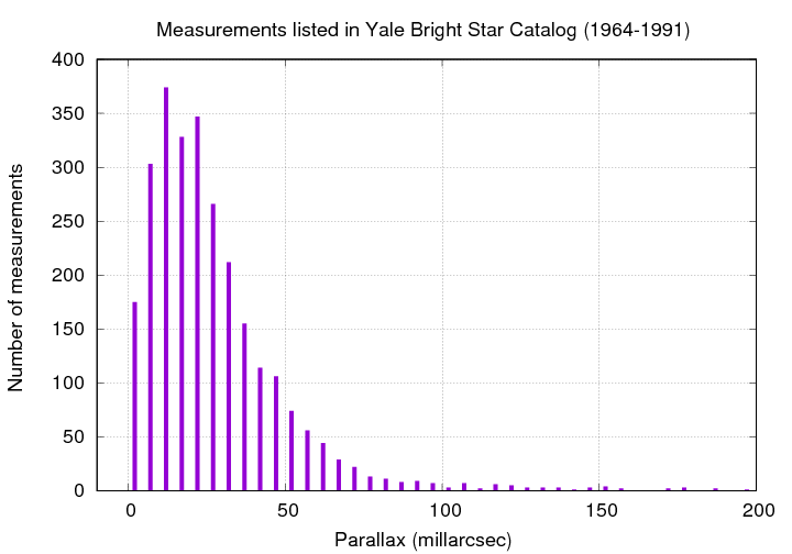
The fact that this histogram turns over below 15 mas is a sign that the precision of the typical measurement is . about 15 mas.
The annoying nature of errors in parallax measurements: part I
It turns out that the nature of parallax measurements means that the connection between the error in the measurement and the error in the distance is not simple. There are a number of tricky aspects which can make the analysis of, say, the possible bias in some catalog, a complicated matter.
The first big problem is that the quantity of interest, the distance to a star d, is INVERSELY related to the measured angle π.
This means that an error of (for example) 20 percent in the measurement does NOT mean that there will be an error of 20 percent in the computed distance.
Why not? Well, let’s do an example to find out. Suppose that we measure the parallax to a star to be

If the uncertainty is the usual «1-sigma» variety, then this measurement means that the true value of the parallax angle has a 66% chance of lying in the range 80 to 120 mas.
Fine so far. But what does that mean for distance we derive from this angle? We need to calculate the distance corresponding to the angle (100 — 20) and the angle (100 + 20). I’ll let you fill in the table below.
The fundamental issue here is that a realistic, symmetric error in the measured angle leads to an ASYMMETRIC error in the derived distance. The larger the fractional error in parallax angle becomes, the more asymmetric this error in the derived distance. For example, if we measure
then the range of distances consistent with the measurement at 1-sigma looks like this:
We can sum up this first problem: symmetric errors in a measured parallax angle lead to asymmetric errors in the derived distance . with a larger range of possible true distances on the «farther away» side.
The annoying nature of errors in parallax measurements: part II
The really nasty bit of the errors-in-parallax discussion is a consequence of the first conclusion: symmetric errors in angle lead to asymmetric errors in distance. Let’s go back to this example again:
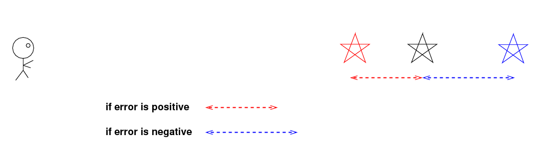
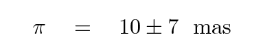
Based on the parallax angle π = 10 mas, we derive a distance of d = 100 pc — but due to the uncertainty in the angle, the true location of the star has a 66% chance of lying anywhere within the range of 59 — 333 pc.
What that means is that the TRUE location of the star could be here .

In fact, the star could lie anywhere along a line in this direction, with equal probability, based on that one measurement. In a one-dimensional universe, the probability that the TRUE location of the star is farther than 100 pc is larger than the probability that the star is closer than 100 pc, simply by the ratio of the lengths of the possible locations:
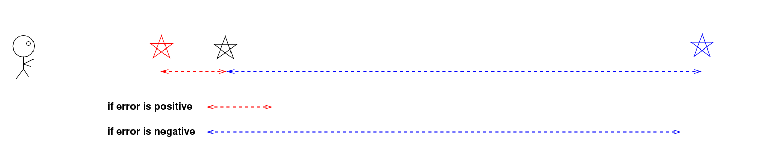
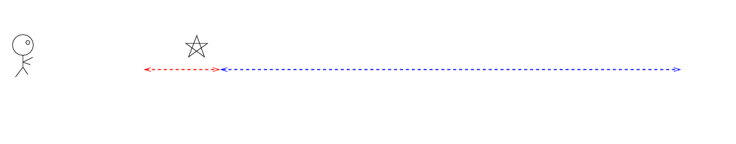
In a TWO-DIMENSIONAL universe, the probabilities would change because the region in which a «farther-than-100-pc» star could exist becomes much larger than that of a «closer-than-100-pc» star.
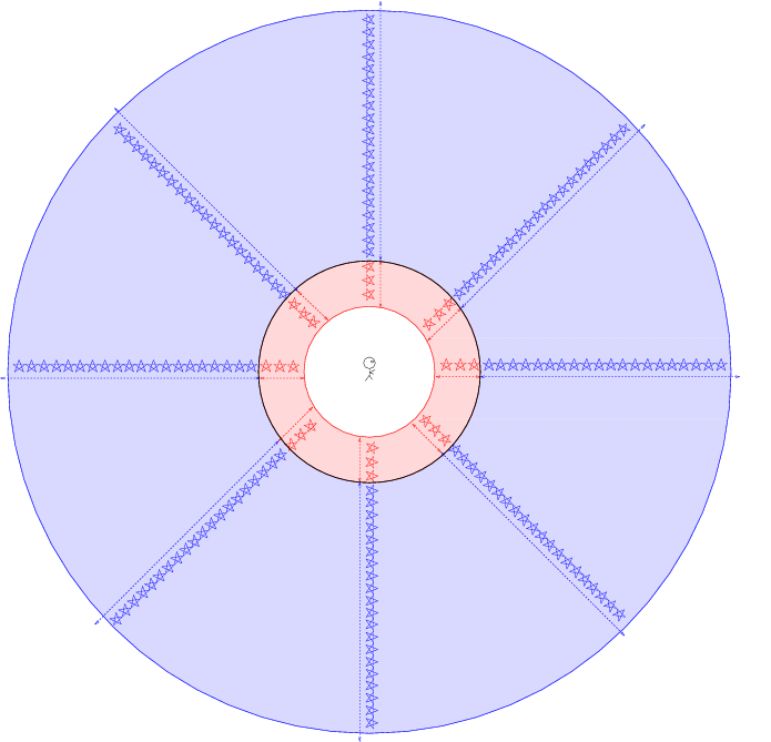
Our course, our real universe is THREE-DIMENSIONAL. Sorry, I can’t draw a good 3-D figure showing the two regions, but I hope you can extrapolate from the two-dimensional case to the three-dimensional one.
Now, what’s the big deal about all of this? The big deal is that we live in a region of relatively uniform stellar density. In our neighborhood of the Milky Way, there are roughly equal numbers of stars in all directions: left, right, up, down, forward, back. Yes, there tend to be more stars in the plane of the Milky Way, but the thickness of the disk is (until Gaia) larger than typical distance we could measure via parallax, that doesn’t really matter.
And so, suppose that we measure the parallax to a star to have the value 10 +/- 1 mas, corresponding to a measured distance of 100 pc. But there are three possibilities for the TRUE distance to this star:
- the star could actually be closer to the Earth, but a negative error in the measured parallax (taking a true value of 11 mas to measured value of 10 mas) makes it appear to be farther away
the star could actually be at exactly 100 pc
Which of these is most likely? The answer is «C». Because there are more stars in the «more distant» volume, it is more likely that a distant star has been improperly measured than a nearby star. The result is that our measurements of parallax lead to a systematic bias: stars appear closer than they really are (sort of like dinosaurs.)
This effect was noted long ago, by Trumpler and Weaver (1953), among others, but Lutz and Kelker first analyzed it detail in 1973. Astronomers sometimes refer to this bias, or the corrections needed to account for it, as the «Lutz-Kelker effect.»
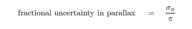
The size of this bias depends (mostly) on the ratio of the uncertainty in parallax to the value of parallax:
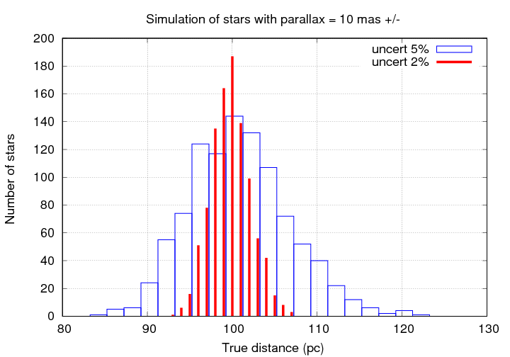
Let’s look at some examples. We will observe a set of stars with measured parallax angles of exactly 10.0 mas, which means measured distances of exactly 100 pc.
When the fractional error is very small — just a few percent — then the errors in the derived distances, and the overall bias, are pretty small.
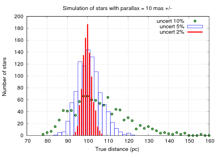
But as the fractional uncertainty grows, the errors and bias increase. Even uncertainties of just 10% can cause big mistakes in the measured parallax. Notice the long tail of true distances out to 140 pc and beyond; the errors in those derived distances are 40 percent or more, far larger than the 10% uncertainty in the parallax angle itself.
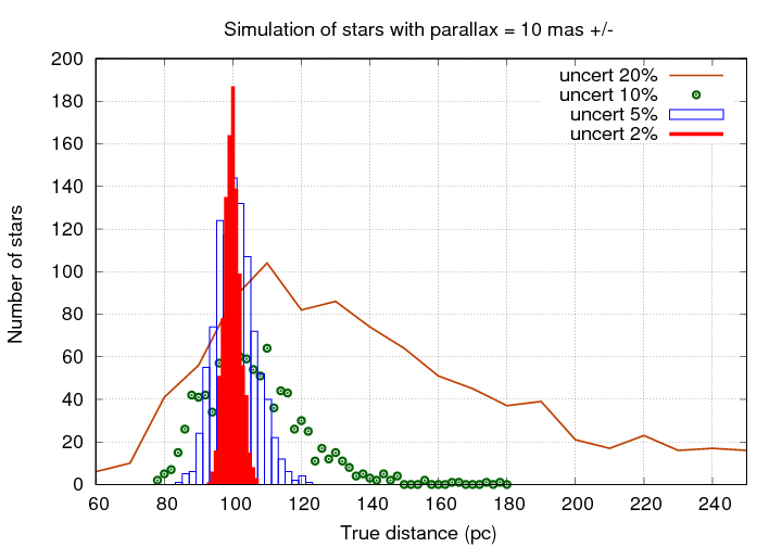
If the uncertainty becomes 20% or larger, the results involve errors which are frequently a factor of 2 or more. No one should try to use such measurements for any careful calculations.
Things are just silly when the uncertaity is 30%!
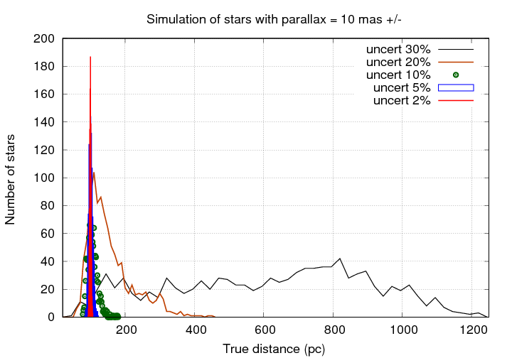
This table summarizes the results of a simulation in which I created a region of space with uniform stellar density, «measured» enough stars to find 1000 falling within a particular range of parallax values around 10 mas, and then compared those «measured» distances to the actual distances.
The moral of this story is — don’t trust distances based on parallax unless the uncertainty in the measurement is much smaller than the measurement itself. I would prefer not to rely on any measurements in which the fractional uncertainty is larger than 10 percent.
How far can it reach? (Classical, again)
Phew. Now that we understand the weaknesses of the parallax method, we can try to answer this question. If we adopt as a general rule that most ground-based measurements of parallax had uncertainties of about σπ = 10 mas, then we can place a very rough limit on the distances of stars derived from such measurements:
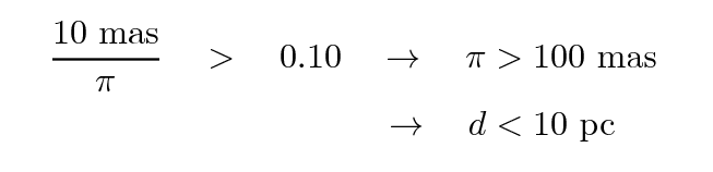
Gosh, that’s not very far.
Of course, astronomers DID use parallax measurements which were considerably smaller than 100 mas; scientists are always interested in pushing the limits of their data. But this is a warning that any statistical inferences based on ground-based measurements of stars at greater distances must be very carefully considered, and corrections must be made for the Lutz-Kelker effect.
How far can it reach? (Hipparcos)
The Hipparcos satellite was launched in 1989 and its first catalog was released in 1997. This project immediately improved our knowledge of stellar distances (and motions, and luminosities) by a large amount. Not only did it cover the entire sky, and measure stars fainter than those typically found in parallax catalogs (down to about mag 10), it also had a typical precision of about 2 mas. In other words, its typical measurement was about as good as the very best ground-based measurements.
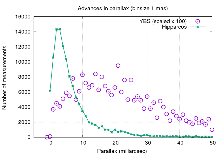
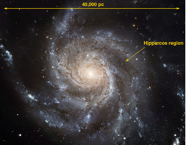
Image of M101 courtesy of NASA, ESA, K. Kuntz (JHU), F. Bresolin (University of Hawaii), J. Trauger (Jet Propulsion Lab), J. Mould (NOAO), Y.-H. Chu (University of Illinois, Urbana), and STScI; Canada-France-Hawaii Telescope/ J.-C. Cuillandre/Coelum; G. Jacoby, B. Bohannan, M. Hanna/ NOAO/AURA/NSF
One of the wonderful results of Hippacos’ measurements were the very accurate HR diagrams which could finally be made, since we now had LOTS of distance measurements to stars of all types. Below is one made using Hipparcos stars with uncertainties of ≤ 10% in their parallax angles.
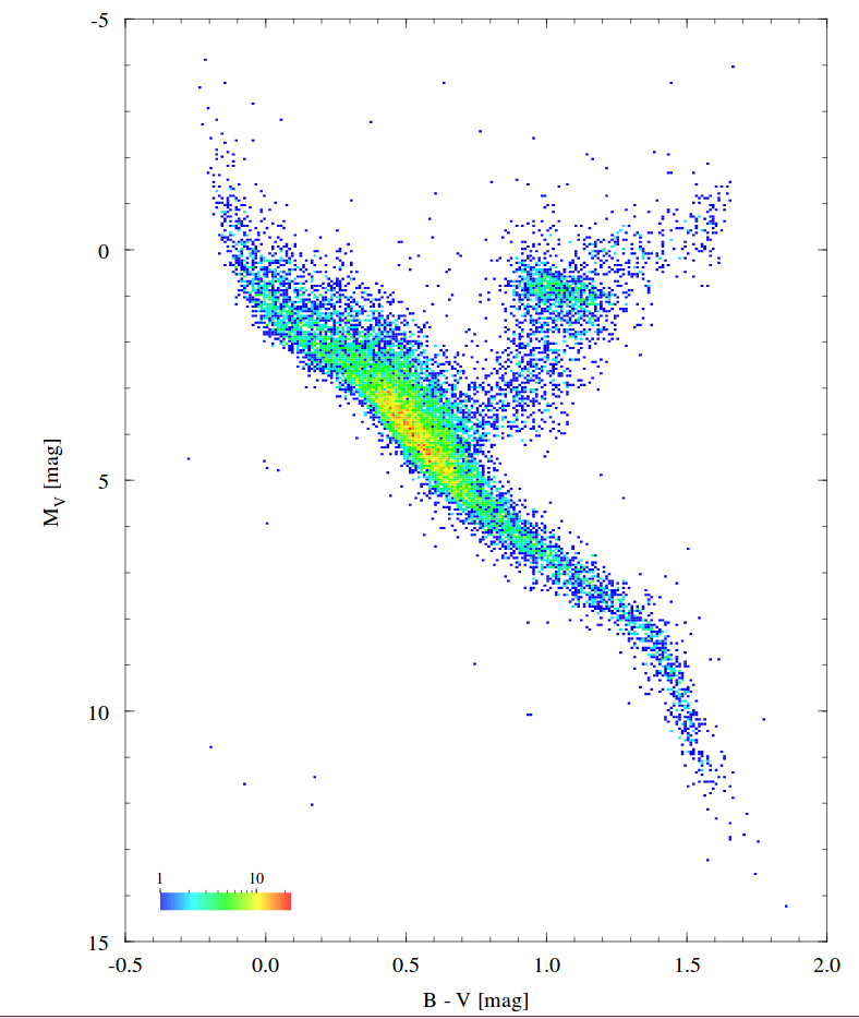
Image courtesy of ESA’s page with HR diagrams based on Hipparcos data.
How far can it reach? (Gaia)
Gaia is a rather unusual «telescope,» since it has been specially designed for astrometric observations. It resembles the Hipparcos satellite in many ways. The basic structure is built around two triple-mirror telescopes which point at regions in the sky separated by an angle of about 106.5 degrees.
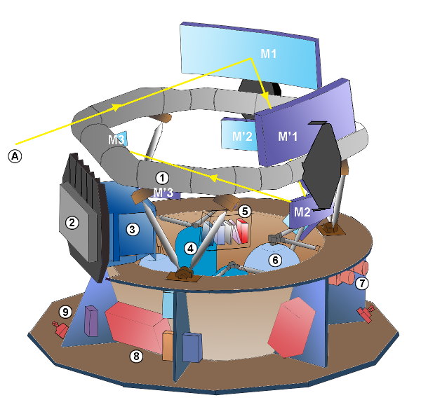
Image courtesy of Wikipedia
Light from the two telescopes is combined so that it falls upon the focal plane simultaneously. The telescope rotates with a period of six hours, causing stars to sweep across this focal plane in about 60 seconds. Objects in both directions are detected and measured together.
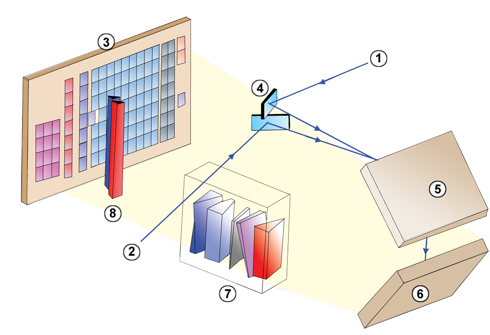
Image courtesy of Wikipedia

Figure 1 from Lindegren et al. 2016. Note that this figure is rotated by 180 degrees relative to previous schematic. The original caption follows.
Layout of the CCDs in Gaia’s focal plane. Star images move from left to right in the diagram. As the images enter the field of view, they are detected by the sky mapper (SM) CCDs and astrometrically observed by the 62 CCDs in the astrometric field (AF). Basic-angle variations are interferometrically measured using the basic angle monitor (BAM) CCD in row 1 (bottom row in figure). The BAM CCD in row 2 is available for redundancy. Other CCDs are used for the red and blue photometers (BP, RP), radial velocity spectrometer (RVS), and wave- front sensors (WFS). The orientation of the field angles η (along-scan, AL) and ζ (across-scan, AC) is shown at bottom right. The actual origin (η, ζ) = (0, 0) is indicated by the numbered yellow circles 1 (for the preceding field of view) and 2 (for the following field of view).
The telescope slowly precesses, so that its spin sweeps out new areas in the sky over time. A typical star will be measured about 70 times over the course of the primary mission (2014 — 2019); that’s about 14 measurements per year, though not all equally spaced.
Image courtesy of Space Flight 101
As the spacecraft precesses, the «partners» of each star will gradually change. Eventually, the spacecraft will have many millions (billions?) of measurements of the relative positions of millions of stars. Scientists can then use a honking-big linear algebra procedure to solve simultaneously for the positions and motions of each star.
How precise are the measurements made by Gaia? As described in Lindegren et al. 2016, the Gaia Data Release 1 consists of a limited set of measured properties for a very limited set of bright stars. Later releases will contain (much) better data for (many) more stars.
Image of M101 courtesy of NASA, ESA, K. Kuntz (JHU), F. Bresolin (University of Hawaii), J. Trauger (Jet Propulsion Lab), J. Mould (NOAO), Y.-H. Chu (University of Illinois, Urbana), and STScI; Canada-France-Hawaii Telescope/ J.-C. Cuillandre/Coelum; G. Jacoby, B. Bohannan, M. Hanna/ NOAO/AURA/NSF
Gaia provides astronomers with many, many more stars than Hipparcos did, so it is possible to create much more detailed HR diagrams:
As time passes, and Gaia continues to scan the skies, it will build up larger and larger sets of measurements of each star, allowing it to create a better solution for the position, parallax, and proper motion of each object. A recent paper by de Bruijne, Rygl and Antoja provides some predictions for the FINAL Gaia precisions.
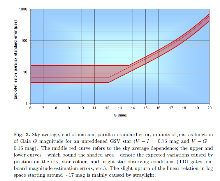
Fig 3 taken from de Bruijne, Rygl and Antoja (2015)
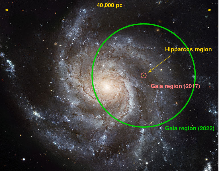
Image of M101 courtesy of NASA, ESA, K. Kuntz (JHU), F. Bresolin (University of Hawaii), J. Trauger (Jet Propulsion Lab), J. Mould (NOAO), Y.-H. Chu (University of Illinois, Urbana), and STScI; Canada-France-Hawaii Telescope/ J.-C. Cuillandre/Coelum; G. Jacoby, B. Bohannan, M. Hanna/ NOAO/AURA/NSF
In any case, Gaia will greatly increase our knowledge of the stellar neighborhood. It will produce a catalog of roughly 100 million stars with distances good to about 10 percent. The Hipparcos catalog contains only 0.12 million entries, of which only about 0.04 million satisfy the Lutz-Kelker criterion.
Let’s look at the timeline for Gaia operations and data releases.
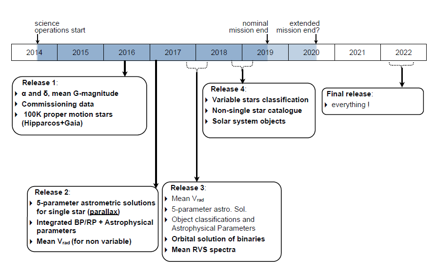
Figure 8 taken from Eyer et al., 2015
Hipparcos vs. Gaia: The case of RR Lyr
As we will see in a future lecture, the star RR Lyrae is a very important one. It is one of the nearest and brightest of a class of pulsating stars which can help us to measure distances not only within the Milky Way, but to other galaxies.
Clearly, if we wish to use the class of RR Lyr stars as distance indicators, we need to know very precisely how luminous they are . and, so, how far away they are. Let’s consider the star RR Lyr itself.
Use the Vizier interface to the Gaia ‘TGS’ catalog to find the distance to RR Lyr
Do the two distances agree within their 1-sigma uncertainties?
This is, of course, just one star. But if our estimates of the distances to other stars, and other galaxies, depend upon RR Lyr stars in particular, and if the new Gaia data suggests that our old value might be incorrect by such an amount . well, that should make you start to worry about the upper rungs on the Cosmological Disetance Ladder!
Hipparcos vs. Gaia: The general trend
Based on the earlier discussion of errors in parallax , we might expect that the Hipparcos measurements, with their larger uncertainties, would show a systematic bias relative to the more precise Gaia values. Let’s put that to the test.
I went to the Gaia DR1 archive site and chose the «ADQL Search Form», which allows the user to enter SQL-like queries to a number of catalogs.

Into the query box, I entered
The result was a set of about 93,000 stars measured by both Hipparcos and Gaia. I then compared the parallax values on a star-by-star basis. As the graph below shows, Gaia and Hipparcos do agree very well, on average: the red dots are individual stars, and the blue symbols are medians within bins of width 1 milliarcsec.
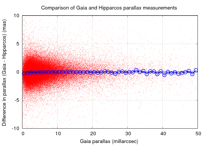
If we zoom in, however, we can see some asymmetry: the Gaia parallax angles tend to be SMALLER than the Hipparcos angles, and the difference grows as the angles decrease in size.
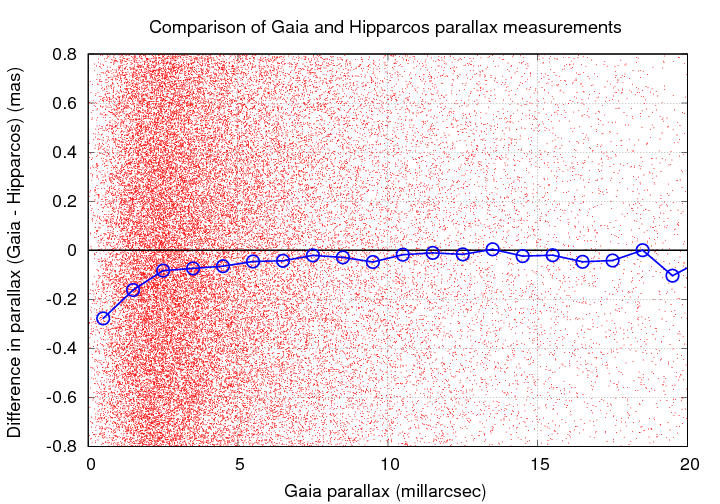
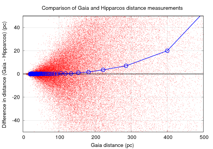
In other words, since the Hipparcos angles are slight OVER-estimates (due to the Lutz-Kelker bias), the Hipparcos distance values tend to be UNDER-estimated as on approaches the limit of its measurements.
We can see that clearly if we plot DISTANCES on our graph instead of angles.
What about radio measurements?
Of course, optical telescopes are not the only ones which can make parallax measurements. Any telescope on (or around) the Earth will share the annual journal, and so have a chance to measure the parallactic shifts of celestial sources.
Stars emit most of their energy in the optical region of the spectrum, and very little in the radio; it isn’t possible to detect most stars with radio telescopes. Clouds of gas and dust do emit plenty of radio waves, but they are for the most part large, extended sources, not the compact objects one requires for parallax measurements.
However, there are some circumstances which do allow radio astronomers to apply the power of interferometry to make very precise measurements of the positions of compact radio sources, and therefore to determine the distances to those sources via parallax. The key element is the maser emission from small clumps of gas within some star-forming regions. Astronomical masers arise within compact volumes, thus appearing as point sources to our radio telescopes, and produce radiation of very pure frequency. The combination allows astronomers to determine their positions with very small uncertainties.
One example of parallax measurements in the radio regime is provided by the Japanese VERA project. VERA is a array of four radio dishes stretched out across the Japanese archipelago.
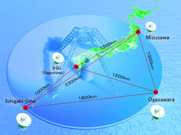
Image courtesy of The VERA group and the National Astronomical Observatory of Japan
If one looks at star-forming regions, such as S269, with an optical telescope, one sees clumps of stars immersed in gas and dust. If one looks with a radio interferometer, one can see much finer details. Compare the scales on the IR picture at left with the VERA map at lower right.

Image taken from a presentation by Mareki Honma, NAOJ
If one measures the position of one of these masers over a period of several years, one will see an intriguing pattern. Shown below are VERA measurements of a maser in the Orion-KL region; the figure shows the Right Ascension component of the position as a function of time.
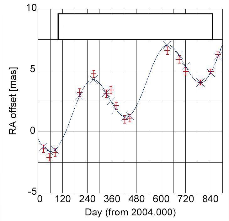
Figure taken from a presentation by Mareki Honma, NAOJ ; I’ve erased the parallax result so that my students can’t peek at it in class.
A slightly more recent measurement by VERA yields the even more precise parallax to Orion-KL of
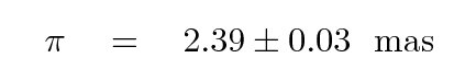
Now, if VERA can measure parallax with a precision of 0.03 mas, then it can reach far out into the Milky Way, too. In fact, at the moment, VERA is one of our best tools for measuring distances in the Milky Way, beating Gaia quite handily.
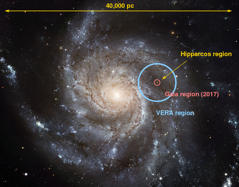
Image of M101 courtesy of NASA, ESA, K. Kuntz (JHU), F. Bresolin (University of Hawaii), J. Trauger (Jet Propulsion Lab), J. Mould (NOAO), Y.-H. Chu (University of Illinois, Urbana), and STScI; Canada-France-Hawaii Telescope/ J.-C. Cuillandre/Coelum; G. Jacoby, B. Bohannan, M. Hanna/ NOAO/AURA/NSF
For more information
- One of the lectures in my course on extragalactic astronomy and cosmology discuss parallax:
- The AU, parallax, and other geometric methods
Way back in the late 1990s, I discussed parallax and the (at that time) exciting new results from Hipparcos. You might find some of the illustrations of the «raw-ish» data from Hipparcos useful.
- Of course, you will want to get your hands on the real Gaia measurements. You have several choices:
- Vizier catalog I/337 provides interactive searching and plotting access to Gaia’s TGAS catalog. I find TGAS more useful than the other Gaia DR1 products, since it includes parallaxes and proper motions.
- The Gaia DR1 release page presents information about this data release, with pictures and statistics and links to many resources.
- The Gaia archive web page has links to the actual catalog interfaces.
- I gathered some material on VERA for a public talk — perhaps it might be useful for reference:
- A talk from 2008 featuring some results from VERA
 Copyright © Michael Richmond. This work is licensed under a Creative Commons License.
Источник
The parallax error is one that occurs when a measurement is made from different viewing angles. A simple example of what is meant by parallax is seen when we close the left eye in front of an object, and then immediately open the left eye and close the right eye: the object will appear to have moved to the right. But when we have both eyes open, we will see the object in the middle.
The same phenomenon can be repeated by positioning our eyes at different angles to an object, such as a simple point (image below). If we wanted to place this point on a ruler, we would make a parallax error when viewing it from the positions marked by the X’s in red.
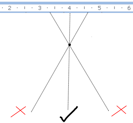
From the X on the right the point will appear to be further to the left, so its location with respect to the ruler is closer to 3 than to 4. Meanwhile, the opposite occurs from the X on the left: now the point will appear to be further to the right, placing it closer to 5 on the ruler.
To avoid parallax error in such measurements, it is always necessary to place the eyes in the most vertical position possible with respect to the scale of the instrument or material.
Parallax error in the laboratory
In the image above we had a scale, the point being a needle, a pointer, the edge of an object, the meniscus of a liquid, etc. That is, we have a scale on which we want to make a reading. Very similar as it happens with the hands of the clock when we read what time it is.
In a laboratory we have scales that offer hundreds of instruments or materials made of glass or metal. When a student makes a measurement that includes direct scaling, he is subject to making parallax errors, which is random: he constantly varies the angle from which he observes or takes the measurement.

Sometimes because of the rush and wanting to write down a reading, the student does not realize that he is making the parallax error, since it does not only occur from left or right angles; also from above or below, and there may be even other angles. You should always take the time to fix your eyes in the most upright and frontal position when comparing an object against a scale.
That is to say, in the laboratory the eyes must be as far as possible in front of the object of our measurements. Otherwise, the accuracy will suffer.
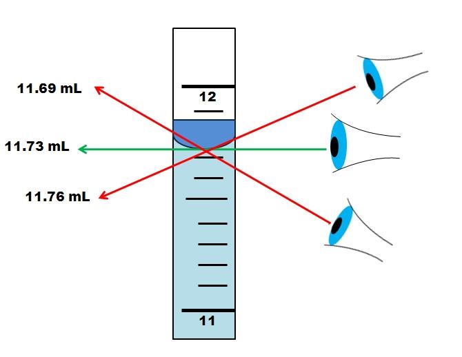
In chemistry laboratories we have in particular the parallax error in volume measurements. For this, there are glass materials such as the graduated cylinder or the burette, each with its own scales (think of a ruler but cylindrical and made of glass).
The liquid within these materials, to say the water, tends to form a concave meniscus (sunken like a valley) on the surface. The base of the meniscus should be compared to one of the closest lines on the scale. However, this comparison is sensitive to parallax, as seen in the image above.
Depending on where and from what direction we want to see the meniscus, its apparent position on the scale will be different. Viewed from below, the meniscus will be lower (11.69 mL) than it is. But viewed from above the meniscus will now appear higher on the scale (11.76 mL).
The real volume (11.73 mL for our example) will be the one that we measure with the eyes (both) in a position as frontal and vertical as possible with respect to the glass material. As you will see in the examples section, there are many operations that generate parallax errors in a chemistry laboratory.
Parallax error in physics
Laboratories
In physics laboratories, on the other hand, volumes can also be measured, but other instruments are of greater importance in their practices.
For example, it is necessary to determine the dimensions, such as lengths and width of an object, using the micrometer (palmer) or the vernier. These instruments have their own scales, which are once again subject to parallax error.

Likewise, if these instruments are analog, we will have ammeters (current meter), ohmmeters (electrical resistance meter), barometers (atmospheric pressure meter), as well as many others, each with scales sensitive to parallax error.
In them, a needle or pointer will move along the scale, whose tip will indicate the appropriate reading as long as we fix our eyes as close and frontal as possible.
Astronomy
In the world of astronomy, parallax has a very special function: to measure distances between celestial bodies, such as planets and stars.
If you place a finger in front of your nose and close and open one eye at a time, you will notice how the finger appears from one side to the other. But this effect diminishes if it is repeated with the finger as far away from the face as possible. The closer a body is, the greater its parallax; and therefore the error that can be made by observing it is greater.
This is the basis for the use of parallax to determine how far away celestial bodies are: comparing the relative positions of two stars from different angles.
Examples of parallax errors
Wall Clock
If we read the time by looking at the wall clock from the left or right, we will get an incorrect time for several minutes. To see the correct time, the hands of the clock must be seen from the front.
Thermometer
Inside the thermometer there is a rising or falling liquid whose meniscus equals a temperature scale. If we view this meniscus from above or below, we will get incorrect temperatures. The thermometer must be viewed from the front and as vertical as possible.
Speedometer
Whoever drives can know precisely what the speed of the car is. However, the copilot (on the right) will see that the needle points at a speed apparently higher than the actual speed.
Preparation of solutions
When a solution is to be gauged, it must be done with the eyes just in front of the gauging line, because otherwise a parallax error equal to that of the thermometer will be repeated.
Analog blood pressure meter
Very similar to the case of the clock, or that of a stopwatch, is that of the blood pressure meter, whose needle must be seen from the front or it can be concluded that the pressure is lower or higher than the real one.
Granataria balance
In the granatary scales you have to read the readings from the front, because the same parallax error that occurs in, for example, school rules would be committed. Reading from the front the true mass of the object in question is obtained.
What is parallax error and why does it matter? Jim Tyler explains what causes parallax error in your scope, why it matters, and how to avoid it!

The term ‘parallax error’ is used to describe movement of the viewed image through a scope relative to the reticle, caused by a change in the position of the user’s eye relative to the axis of the scope. Put simply, the position of your intended pellet point of impact (POI) moves away from the reticle aim point if your eye moves away from being directly behind the axis of the scope. Parallax error is thus a potential cause of inaccuracy.

Simple Equation
The distance by which the image of the intended POI can move away from the reticle aim point can be calculated using a very simple equation, which is the radius of the objective lens multiplied by the difference between the target distance and the scope focus (parallax) range, and divided by twice the focus range.
A 40mm objective lens scope parallax focused at 25 yards and with a target at 40 yards has a maximum potential shift of 20 x 15/50, which works out at 6mm. That means the pellet can land a maximum of 6mm – in any direction according to whether your eye is left, right, high or low – away from the intended POI, and it’s important to realise that this figure is the absolute maximum, to achieve which, your eye must be a long way from the centre of the scope, much further than you’ll normally achieve unless you make a special effort to look through the edge of the image.

Experimental evidence
Experiments suggest that unless you do make a deliberate effort to move your eye as far from the scope axis as possible, parallax POI shift, in practice, is likely to be nearer a quarter of the absolute maximum, or 1.5mm, which isn’t a lot unless you’re a paper-target shooter.
There are ways in which the POI error caused by image shift can be reduced, or even negated, but before looking at them, we’ll consider what exactly causes the image shift that can lead to parallax error.

Focus
All the light we see when viewing a target in daylight emanates from the sun, and has reflected from the surface of the target. The light from a single point on the target bounces off in many directions, some of it entering the entire surface of the objective (front) lens of a telescopic sight; refracting (passing through) each air/glass boundary causes the light to bend, and the objective when focusing a scope for parallax purposes is to get all of the light from that single point on the face of the target to converge at a single point, at the plane of the reticle. When this is achieved, the light from that single point or any single point on the target, for that matter, will always appear in exactly the same place relative to the reticle, and parallax error simply cannot occur, no matter how far from the axis of the scope you place your eye.

Focusing systems
Sounds good, but there’s a fly in the ointment, which is that it is not straightforward to get the light to converge exactly at the plane of the reticle; before looking at that, a quick look at the means of focusing the scope.
Some scopes have one of two mechanisms for focusing the objective lens; the first to appear was an adjustable collar surrounding the objective bell, which is connected to the objective lens carrier, and can be screwed in and out to move the objective lens, and hence the point at which the light from a single point converges, back and forth. Scopes with this mechanism are usually advertised as PA (parallax adjustable).
The other, more recent, focus method is a wheel mounted on the side of the turret, which moves a lens or lenses in a carrier inside the scope to move the point of convergence back and forth, and these are usually advertised as SF (side focus). Both mechanisms do the same job, and the only advantage of the SF is that it’s arguably easier to adjust while looking through the scope.

The fly in the ointment
Remember I mentioned a fly in the ointment? Well, it is not enough for the light from the target to converge at the reticle, it also has to pass through the lens of your eye and converge again at a single point on your retina, and herein lies the potential problem.
The scope focus mechanism that controls the point of convergence in your eye is the ocular focus, at the rear of the scope, and it is necessary because our eyes are not all exactly the same.
The usual advice for focusing the ocular lens is to point the scope at a plain area of sky, and turn it until the image of the reticle is at its sharpest. The problem with doing it that way is that your eye has autofocus, and your eye might force focus with the plain background, but when your eye focuses instead at the image of a target, the reticle might consequently not be at its sharpest – you probably won’t notice it because you’re concentrating on the image of the target – because the light is not converging on your retina, and the consequence can be parallax error.
The right way
Set the ocular focus as best you can using the method described above, and set a target out at your chosen (parallax) focus range.
With your scope at its maximum magnification (to reduce depth of field, which makes it easier to judge when it’s in focus), point the scope at the target and adjust the front focus until the image is at its sharpest; then, taking care not to move the scope, move your head and see whether the image moves. If it does, readjust the ocular focus and try again, repeating until the image does not move relative to the reticle. The scope is now properly focused.
Other means
Hunters and field-target shooters can adjust focus to the range of every shot, but HFT shooters are not allowed to alter scope settings once they have started a course, and like those of us who use scopes that do not have a focus mechanism, they can reduce the potential for parallax error by other means. The key is always to look through the same part of the scope, preferably the centre, although what’s important is consistency. This can be achieved through practising whilst concentrating on head position until it becomes second nature, although that’s easier said than done in the three positions used in HFT.
More help
There is something else that can help limit parallax error, and that is proper gun fit. Few airguns have stock combs the right height for scopes held in high, medium or, in some cases, even low mounts, so they aren’t much help in trying to achieve consistent eye placement. The ideal, although most expensive solution is to have a custom stock tailor-made to suit you, or if you have the necessary skills, to make your own. A tailor-made stock won’t just help to reduce parallax error, but will also help with cheek weld and generally make your hold more consistent.
Cheaper option
A less expensive alternative is to have the comb cut from the stock, then refitted with riser bars that allow you to set the height to suit you. This has the advantage that if you come to sell the rifle or stock, the buyer can adjust it to suit him or herself.
The cheapest option is only for the brave, and it entails planing the comb level, glueing on a block of wood and reshaping it. I did this to a couple of stocks with good results many years ago, but these days, I’m not so brave.
Conclusion
In theory, parallax error can be significant, but in practice and with a little care, it can be minimised.
Parallax error is the error that is most committed when readings are taken in physics. You can thus understand why it is important to avoid it at all cost. One must be aware of its existence at all time so that it can be avoided and as a result the true value of the reading is obtained.
The concept of parallax error is related to the term parallax.
Imagine that we have in a room a pelican and a flamingo as shown in fig 1 below.
![clip_image004[10]](https://lh5.ggpht.com/_MLcxcpYx4ws/SzGUePOvPyI/AAAAAAAAAQ4/8JYZbH7-GVA/clip_image00410_thumb2.gif?imgmax=800 "clip_image004[10]")
Fig 1
Now Garfield is moving about in the room and each time is is somewhere in the room, he looks at the two birds. At the point A he sees the flamingo on the left of the pelican whereas when he is at position C he would see the flamingo on the right of the pelican. Only when he would be at position B would he sees the two birds one behind the other.
He would discover that each time he is at a different position, he would find that the position of the flamingo relative to the pelican has changed.
You can also have this effect when you are in front of a clock. If you move from side to side you would find that the time that you can read from the clock is different.
So we can the understand that the parallax is the change in the apparent position of an object when the position of the observer changes.
Now let us look at the concept of parallax error. If you have placed a pencil on a metre rule and you are reading its length then just like in fig 1 above and in fig 2 below you can place you eye everywhere you want.
![clip_image002[13]](https://lh3.ggpht.com/_MLcxcpYx4ws/SzGVMDClCrI/AAAAAAAAARA/3dGdBJwo_90/clip_image00213_thumb2.gif?imgmax=800 "clip_image002[13]")
Fig 2
As you can see from fig 2 above I have chosen three position at which you can place your eye.
Clearly at these three position we can have the following reading
Reading at A = 6.2 cm
Reading at B = 5.8 cm
Reading at C = 5.5 cm
What you you think would be the correct reading?
The correct reading is would be obtained when the eye is placed at B.
![clip_image002[15]](https://lh3.ggpht.com/_MLcxcpYx4ws/SzGVlrK7VLI/AAAAAAAAARI/r6JXK9GcBr0/clip_image00215_thumb1.gif?imgmax=800 "clip_image002[15]")
Fig 3
Now there is a line from the tip of eye to the of the pencil that continues up to the scale. this line is called the line of sight and the mark at which the line intersect the scale is the length of the pencil. This line of sight must be be at right angle to the scale. This is shown above in fig
If the line of sight and the scale are not ar right angle to each other then a parallax error is committed.
Similarly with a measuring cylinder the line of sight from the eye to the bottom of the meniscus must be at right angle to the scale as shown in fig 4 below. In this case the line of sight is horizontal and the scale vertical.

Fig 4
So as you can see above each time you are taking a reading you must ensure that the line of sight is perpendicular to the scale.
A measuring equipment can give precise but not accurate measurements, accurate but not precise measurements or neither precise nor accurate measurements.

Accuracy is a measure of how close the results of an experiment agree with the true value.
- When there is high accuracy (accurate shots), there will be small systematic error
- The accuracy of a reading can be improved by repeating the measurements.
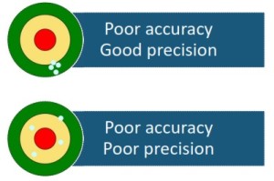
Precision is a measure of how close the results of an experiment agree with each other. It is a measure of how reproducible the results are.
- High precision implies a small uncertainty and small random error.
- Precision is how close the measured values are to each other but they may not necessarily cluster about the true value.
- Zero errors and parallax errors affect the precision of an instrument.
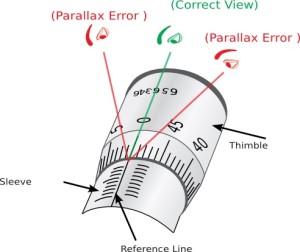
Parallax Error
For accurate measurement, the eye must always be placed vertically above the mark being read. This is to avoid parallax errors which will give rise to inaccurate measurement.
Parallax errors affects the accuracy of the measurement. If you consistently used the incorrect angle to view the markings, your measurements will be displaced from the true values by the same amount. This is called systematic error.
However, if you used different angles to view the markings, your measurements will be displaced from the true values by different amounts. This is called random error.
Parallax error for micrometer screw gauge:
Zero Error
Zero Errors of Vernier Caliper
When the jaws are closed, the vernier zero mark coincides with the zero mark on its fixed main scale.
Before taking any reading it is good practice to close the jaws or faces of the instrument to make sure that the reading is zero. If it is not, then note the reading. This reading is called “zero error”.
The zero error is of two types:
- Positive zero error; and
- Negative zero error.
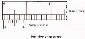
Positive Zero Error (Vernier calipers)
If the zero on the vernier scale is to the right of the main scale, then the error is said to be positive zero error and so the zero correction should be subtracted from the reading which is measured.
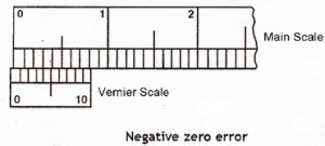
Negative Zero Error (Vernier calipers)
If the zero on the vernier scale is to the left of the main scale, then the error is said to be negative zero error and so the zero correction should be added from the reading which is measured.
Please refer to “How To Read A Vernier Caliper” for more information.
More Vernier Caliper Practice:
- Without Zero Error
- Finding The Zero Error
- With Zero Error
- With Other Measurement Topics
Zero Errors for Micrometer Screw Gauge
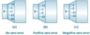
Positive Zero Error (Micrometer Screw Gauge)
If the zero marking on the thimble is below the datum line, the micrometer has a positive zero error. Whatever reading we take on this micrometer we would have to subtract the zero correction from the readings.
Negative Zero Error (Micrometer Screw Gauge)
If the zero marking on the thimble is above the datum line, the micrometer has a negative zero error. Whatever readings we take on this micrometer we would have to add the zero correction from the readings.
Note: You do not have to memorise positive error = subtract, negative error = add, just think this through for a while. It is rather straightforward and intuitive.
Please refer to “How To Read A Micrometer Screw Gauge” for more information.
Self-Test Questions
How can you avoid parallax errors when measuring a length with a metre rule?
The first thing is to place the metre rule such that it’s edge is incident on the length, which will allow easy and accurate reading of the markings on the metre rule. The second thing is to place your eye vertically above the required points – “starting point” and “ending point”.
Electrical and Electronic Measurements
Barrie A. Gregory, Retired, in Encyclopedia of Physical Science and Technology (Third Edition), 2003
I.D Digital Measurements
Most digital instruments display the measurand in discrete numerals, thereby eliminating the parallax error and reducing the operator errors associated with analog pointer instruments. In general, digital instruments are more accurate than pointer instruments, and many (as in Fig. 6) incorporate function, automatic polarity, and range indication, which reduces operator training, measurement error, and possible instrument damage through overload. In addition to these features, many digital instruments have an output facility enabling permanent records of measurements to be made automatically.
Digital instruments are, however, sampling devices; that is, the displayed quantity is a discrete measurement made either at one instant in time or over an interval of time by digital electronic techniques. In using a sampling process to measure a continuous signal, care must be exercised to ensure that the sampling rate is sufficient to allow for all the variations in the measurand. If the sampling rate is too low, details of the fluctuations in the measurand will be lost, whereas if the sampling rate is too high, an unnecessary amount of data will be collected and processed. The limiting requirement for the frequency of sampling is that it must be at least twice the highest frequency component of the signal being sampled, so that the measurand can be reconstructed in its original form.
In many situations the amplitude of the measurand can be considered constant (e.g., the magnitude of a direct voltage). Then the sampling rate can be slowed down to one that simply confirms that the measurand does have a constant value. To convert an analog measurand to a digital display requires a process that converts the unknown to a direct voltage (i.e., zero frequency) and then to a digital signal, the exception to this being in the determination of time-dependent quantities (Section III.C).
The underlying principle of digital electronics requires the presence or absence of an electrical voltage; hence a number of conversion techniques are dependent on the counting of pulses over a derived period of time. Probably the most widely used conversion technique in electronic measurements incorporates this counting process in the dual-slope or integrating method of analog-to-digital (A–D) conversion. This process operates by sampling the direct voltage signal for a fixed period of time (usually for the duration of one cycle of supply frequency, i.e., 16.7 msec in the United States, 20 msec in the United Kingdom). During the sampling time, the unknown voltage is applied to an integrating circuit, causing a stored charge to increase at a rate proportional to the applied voltage, that is, a large applied voltage results in a steep slope, and a small applied voltage in a gentle slope (Fig. 8). At the end of the sample period, the unknown voltage is removed and replaced by a fixed or reference voltage of the opposite polarity to the measurand. This results in a reduction of the charge on the integrating circuit until zero charge is detected. During this discharge period, pulses are routed from a generator to a count circuit, which in turn is connected to a display. The reason for the wide use of this technique in digital multimeters is that, since the sampling time is one cycle of power supply frequency, any electrical interference of that frequency superimposed on the measurand will be averaged to zero.

FIGURE 8. Dual-slope A–D conversion process.
Another A–D conversion technique commonly used in electronic instruments is based on the successive-approximation process. In this a fixed, or reference, voltage is compared with the unknown. If the unknown is greater than the reference (which could have a magnitude of, say, 16 units), this fact is recorded. The reference is then halved in value and added to the original reference magnitude, so that a known value of 24 units is compared with the measurand. Had the unknown been less than 16 units, a comparison between 8 units and the measurand would be made. Fractions of the reference level are added (or not) until an approximation to the magnitude of the measurand is established (within the limits of the available resolution). For the unknown voltage in Fig. 9, the magnitude is 16+8+0+0+1 units or, if represented by a binary chain, 1101 units. The advantage of the successive-approximation technique is that it can be manufactured to have a very short sampling time (less than 1 μsec) and can thus be used for fast analog-to-digital conversions in, for example, waveform recording and analysis.

FIGURE 9. Successive approximation A–D conversion process.
The principal advantage of a digital display is that it removes ambiguity, thereby eliminating a considerable amount of operator error or reading misinterpretation. Unfortunately, it may create a false confidence. The assumption that “I can see it, therefore it must be correct” may not be true due to interference effects, the specified limitations, and the loading effects of the instrument. The modern trend of incorporating programming capability into instruments has created a need for alphanumeric displays rather than a simple numeric display. Figure. 10 illustrates two types of array that are in use in addition to the seven-segment numeric display. The methods used to produce the display are light-emitting diodes (LEDs), liquid-crystal displays (LCDS), gas discharges (Nixie tubes and plasma panels), and cathode ray tubes (CRTs) or, as they are becoming more frequently known, visual display units (VDUs).

FIGURE 10. Digital displays: (a) dot matrix and (b) bar arrangement.
The developments in computing technology have led to the creation of “virtual instruments” where an interface to a laptop or personal computer is used to connect points in a circuit or system and the screen display contains several conventional instrument displays (Fig. 11). These virtual instrument systems vary in complexity from a terminal “pod” to which one or two points in a circuit may be connected and can provide a VDU display of signal magnitude, frequency, spectral analysis, and waveform, to more complex arrangements with plug-in cards that can take 8, 16, or 32 inputs and perform analysis and computations on the signals connected to the plug-in card.
Read full chapter
URL:
https://www.sciencedirect.com/science/article/pii/B0122274105002027
Tools, Cutting Techniques, Risk, Reliability, and Safety Issues
Francis Nickols, Yueh-Jaw Lin, in Creating Precision Robots, 2019
1.2 Marking Out the Cardboard
You need to order black sheets of A2 size and a cardboard of 1.5 mm thickness. This cardboard has an areal density of approximately 1.2 kg/m2, which is useful when estimating the mass of moving parts such as the shuttle in the Catapult Robot.
Marking out should be done with the transparent rule as a first choice as there will be no parallax error because the rule markings are adjacent to the cardboard surface. Whether you use a transparent rule or a steel rule, which has parallax error due to its markings 1 mm above the cardboard surface, you should use the pencil as shown here to reduce any further possibility of parallax error.

After making pencil marks you should draw pencil lines indicating where to cut the cardboard. Keep your pencil upright when viewed from the front as shown here. Remember the pencil lead is 0.5 mm but the metal spout that supports the lead has a diameter of 0.8 mm so if your lead is protruding greater than 1 mm which is the thickness of the rule then you are increasing the likelihood of error. So keep your lead short such that the metal spout is in contact with the rule and the rule is thus 0.8 mm/2 = 0.4 mm away from the pencil marks. It may seem impossible to obtain such precision but you will be surprised that with patience and practice, human eye and hand coordination is surprisingly accurate.

Read full chapter
URL:
https://www.sciencedirect.com/science/article/pii/B9780128157589000018
An Application of HDR in Medical Imaging
G. Ramponi, … G. Guarnieri, in High Dynamic Range Video, 2016
19.4.2 Techniques for Image Splitting
The simplest possible technique is to perform the splitting on a pixel-by-pixel basis. More precisely, if we indicate with Lin(x,y) the luminance of the input image at pixel location (x,y) and follow the notation used in Eq. (19.4), the splitting algorithm takes the form
(19.5)Tb(x,y)=F(Lin(x,y)),Tf(x,y)=Lin(x,y)BTb(x,y).
In other words, we compute the transmittance of the back panel by mapping the input luminance with a suitable nonlinear function F(⋅), and we subsequently compute the transmittance of the front panel by division in order to guarantee that the product of the two images reproduces the input. The splitting is computed on linear data; the nonlinear encoding of the source image (if present) and the response of the liquid crystal panels are compensated appropriately by the mapping of the data before and after the processing. An intuitive choice for F(⋅) is a square root (Penz, 1982): in this way, each panel displays the same image.
If this simple technique is used on an actual dual-layer display, a problem immediately becomes visible. There is a small but not negligible distance between the liquid crystal cells of the two panels, due to the presence of glass sheets and polarizing filters in between. Therefore, if the observer looks at the display from an oblique angle, the two images appear misaligned. More precisely, instead of seeing the correct image Lout(x,y)≜BTb(x,y)Tf(x,y), an observer focusing on position (x,y) on the display surface sees a distorted image L~out(x,y)≜BTb(x+Δx,y+Δy)Tf(x,y), where the displacements Δx and Δy depend on the viewing angle. This form of distortion is the parallax error that was described in Section 19.4.1. It can be proved that in order to minimize the parallax error, a splitting algorithm should minimize the norm of the relative gradient of the back panel (ie, the back panel should be smooth).
However, the back-panel values cannot be generated by a simple low-pass filter, because of limitations in the dynamic range of the panels and the need to obtain a perfect or quasi-perfect reconstruction of the output image (Guarnieri et al., 2008a). One possible solution is to generate, by means of a constrained optimization algorithm, a back panel that minimizes the parallax error and from which a front panel with suitable black-to-white range can be generated. To do so, it is computationally advantageous to minimize the mean squared value of the parallax error, subject to constraints that can be easily derived by the panel specifications. If perfect reconstruction is required, the transmittance of the front panel can be computed by division, as in Eq. (19.5).
An example of splitting of an actual medical image is shown in Fig, 19.3.

Figure 19.3. Example of splitting. From left to right, original image, back panel, and front panel.
Source: Reprinted with permission from Guarnieri, G., Albani, L., Ramponi, G., 2008. Image splitting techniques for a dual layer high dynamic range LCD display. J. Electron. Imaging 17 (4), 043009-19.
Fig. 19.3 shows that the back panel still contains sharp edges. This happens when the input image contains edges which have a greater magnitude than the dynamic range of the panels. In this case, the front panel alone is not able to completely reproduce the edge, and a fraction of its magnitude must be transferred onto the back panel.
One possible solution is to allow some distortion in the visualized image. The properties of the visual system suggest that the details on the dark side of a high-contrast edge are less visible; this can be used to relax the requirement of perfect reconstruction in those portions. As a consequence, the back-panel transmittance Tb(x,y) and the front-panel transmittance Tf(x,y) are no longer linked by Eq. (19.5), and are both treated as unknowns in the optimization problem. The constraints are simple bounds, constant over the entire image:
(19.6)Tmin≤Tb(x,y)≤TmaxTmin≤Tf(x,y)≤Tmax∀(x,y),
where Tmin and Tmax are the black and white levels of the panels.
The reconstruction error metric to be used in this case must satisfy two strongly conflicting requirements. It should be kept as simple as possible, because it is being used inside an optimization algorithm; this excludes advanced methods such as visible difference predictors (Daly, 1993; Mantiuk et al., 2004). At the same time, the expression should be spatially adaptive because, as mentioned above, the eye sensitivity depends on the context.
We can obtain a pointwise estimate of the visibility of the reconstruction error by taking the ratio between the luminance error and the JND. We obtain the JND by mapping the adaptation level Lad with a threshold versus intensity (TVI) function (Ashikhmin, 2002); possible choices for the latter are discussed in Section 19.4.3. In turn, we compute Lad by filtering the input image with a low-pass filter; in this sense the metric is spatially adaptive (in particular, it correctly predicts the lower visibility of the details near brighter portions), but at the same time the computational cost is low. The function to be minimized takes the following form:
(19.7)Etotal=∬kp∇log(Tb)2+Lin2TVI(Lad)2log(Tb)+log(Tf)−logLinB2dxdy,
where kp is a user-adjustable scalar parameter that balances the relative weight of the reconstruction and the parallax errors.
A full analysis of the variational problem (Eq. 19.7) is beyond the scope of this chapter; it can be found in Guarnieri et al. (2008c) together with a discrete formulation of the problem itself and its numerical solution.
Read full chapter
URL:
https://www.sciencedirect.com/science/article/pii/B978008100412800019X
Recent advancements in AC microgrids: a new smart approach to AC microgrid monitoring and control using IoT
P. Madhumathy, Shweta Babu Prasad, in Microgrids, 2022
Abstract
The proposed system shows a novel microgrid (MG) control system that employs the Internet. Recently, in an MG, a person is employed to record for measuring parameters like voltage, current, temperature, and humidity of the transformer and related equipment that influences the transformer along with causing parallax error. Hence, in the proposed system the error that occurs can be lessened to enhance the strength and competence. Here, sensors are utilized to detect the different transformer specifications; this detected information is transmitted to the microcontroller that analyses the necessary values and transmits the values to the liquid crystal display, driver, and RS-232, which is interfaced with the PC or workstation. The gathered information is further transferred by means of the web to the server. Since the reports are conveyed by means of the web, it can be ensured that the legitimate information reaches the authentic individuals. The essence of Internet of Things (IoT) lies in documenting and sharing of crucial information of the network-connected devices via secure service layer. In straightforward terms, IoT is characterized as the wireless connection of devices linked to each other to transmit information for storage and future analysis. IoT gains maximum capacity by utilizing special objects, that is, smart objects that use multiple sensors and actuators that are able to detect parameters in the environment and communicating this to other linked devices through networking capabilities and helps in smart energy management in green cities.
Read full chapter
URL:
https://www.sciencedirect.com/science/article/pii/B9780323854634000022
Preoperative Planning of Endovascular Procedures in Aortic Aneurysms
I. Macía, … L. Kabongo, in Computing and Visualization for Intravascular Imaging and Computer-Assisted Stenting, 2017
5.1.1 Vessel Diameter, Length, and Area Quantification
In both standard and fenestrated endograft sizing, a precise quantification of the vessel diameters and lengths is crucial. Generally, these measurements are estimated from the segmented lumen and the extracted centerline. Usually, the quantification starts from a user-selected input position in the centerline and hence, user variability is introduced.
As the aorta is not a regular cylinder, a proper characterization of its shape and diameters must be made at different anatomical points. Since parallax error affects the representation of the true vessel size on axial slices [34], aortic cross-sections are extracted perpendicular to the centerline, allowing real diameters to be quantified [35, 36]. Moreover, aortic sections are not typically circular, so slightly different strategies for diameter quantification are in the literature. Macía et al. [37] proposed an optimization procedure that converts the vessel measurements into a cost function that is optimized with respect to a set of parameters. In order to obtain the section boundaries, a ray-casting strategy from the section center is used, as defined by the centerline, in order to extract the inner wall artery boundaries estimating maximum, minimum and average diameter for the selected section [8]. Another approach, proposed by Martufli et al. [38] utilizes the fluid mechanics definition of hydraulic diameter.
Vessel length quantification is usually assessed by measuring the distance along the centerline between two anatomic landmarks, thus providing a much more realistic model of the aortoiliac segment than directly measuring on the sagittal and coronal planes [37, 39, 40].
Area measurements can be obtained either automatically, based on lumen segmentation, or manually on perpendicular cross-sections, especially when thrombus and vessel wall areas are to be included. Area measurements are usually presented as a profile or contour shapes along the vessel medial axis.
Read full chapter
URL:
https://www.sciencedirect.com/science/article/pii/B9780128110188000151
Practical Failure Assessment Methods
K. Ravi-Chandar, in Comprehensive Structural Integrity, 2003
7.09.4.1.4 High-speed photography
Perhaps the most important technique for crack speed measurement is the high-speed camera; this has been a very popular although expensive method for dynamic fracture investigations. One major advantage of high-speed photography is that the event is observed without imposing any preconceived models for the interpretation of the observations. Another advantage is that full field optical methods of stress and deformation analysis such as photoelasticity, method of caustics, shearing interferometry, moiré interferometry, and other techniques can be used to augment the crack position data with additional information on the crack-tip deformation and stress fields. While the earliest attempts produced a single image by using a single spark light source, advances in the technology of high-speed photography have enabled camera designs for obtaining multiple images with a high spatial and temporal resolution. Modern high-speed cameras are capable of obtaining high-resolution images at time intervals of the order of 10 ns, with exposure times of the order of 2 ns. Field (1983) provides a good review of the techniques used in high-speed photography; modern high-speed cameras are available from many commercial vendors.
The first high-speed camera to obtain multiple images of crack growth was the Cranz–Schardin multiple-spark camera; in this camera system, multiple-spark light sources are arranged in a square or rectangular array. The object or region of interest is imaged on a camera with multiple lenses, also arranged in the same square or rectangular array as the light source. Each spark then forms a discrete image through its matching lens. Riley and Dally (1969) provide a detailed description of the design, construction, and operation of a Cranz–Schardin camera. Two major limitations exist in the Cranz–Schardin camera system. First, the multiple light sources cannot be aligned with the optical axis and hence a parallax error is introduced in the observations. Second, the duration of the spark sources is ∼0.3 μs; this long exposure time results in an image smear, but for typical crack speeds of ∼103 m s−1, the image quality is quite acceptable since the smear is only ∼300 μm. Large fields of view are possible in this arrangement; the system described by Riley and Dally has a 45.7 cm field of view. The timing between the sparks is controlled independently and hence the images can be obtained at different time intervals, focusing on times where higher data rates may be needed.
Rotating mirror cameras and rotating drum cameras provide an improvement over the Cranz–Schardin cameras in some respects, but not others. The operating principle in these cameras is to transport the image to a different location on the film either by moving the image with a rotating mirror or by moving the film by rotating the drum that holds the film and in some cases through a combination of the two mechanisms. Illumination from a spark light source or from a pulsed laser is used to form discrete images. Parallax errors are eliminated in this arrangement since the light source and the imaging system are aligned along the optical axis. The number of images that can be obtained is increased significantly to more than a 100 frames. However, the size of the frames is usually quite small; this is dictated by the fact that during the interframe time interval the image has to be translated by a distance equal to its size. The speed with which this can be accomplished is limited by resonance phenomena in the turbines used to rotate the mirror or the drum. Typical framing rates that are possible with the rotating mirror or drum cameras are in the range of 103–106 frames per second.
Two new types of electronic high-speed imaging cameras have been developed: the image converter cameras and CCD cameras. In the image converter cameras, the image falls on a photocathode which converts the image to a stream of electrons. These streams are steered to different parts of a phosphorescent screen by deflector plates, forming discrete images; the phosphorescent images are retained for many seconds and are then photographed on standard photographic film. Exposure time is controlled by the flash that illuminates the photocathode, but the framing rate is controlled by the speed of switching of the deflector plates. Therefore, very high framing rates may be obtained with these cameras. The main drawback is that the number of frames that can be obtained is usually quite small, ∼4–12. The spatial resolution is dictated by the phosphorescent screen and is inferior to that achieved with rotating mirror cameras. Multiple CCD cameras have also been introduced; these are not too different from the Cranz–Schardin cameras in that arrays of CCDs are used to obtain multiple images. However, the image is made to fall on the different sensors by using beam splitters thereby eliminating parallax errors. The CCDs are exposed at high speeds but are then read offline at slower speeds. As in the image converters, while high speeds—of the order of 108 frames per second—are possible, the number of frames and the spatial resolution are limited. Typically ∼8–16 frames are available and the image resolution is ∼1,300×1,000 pixels over the image.
One major conclusion from dynamic crack speed measurements that is quite insensitive to the issues involved in the resolution of the different measuring techniques is that the limiting speed is not a fixed fraction of the Rayleigh wave speed, but is material dependent. This points to the fact that while a limiting speed is set by the continuum wave propagation theory, inherent material processes that govern fracture dictate a significantly lower limit. In fact, Schardin (1959) suggested that the limiting speed be considered a new physical constant for materials. Schardin’s paper provides an excellent overview of the early experimental work on dynamic fracture.
Read full chapter
URL:
https://www.sciencedirect.com/science/article/pii/B0080437494070427
Positron emission tomography
Gaspar Delso, … Patrick Veit-Haibach, in Reference Module in Biomedical Sciences, 2022
Compromise between spatial resolution and sensitivity
The spatial resolution of PET is limited by the nature of the positron annihilation process. On the one hand, positrons do not annihilate exactly where they were created, but travel a small distance, known as positron range, which depends on the initial energy of the positron. Also, the emission of two perfectly antiparallel photons is expected due to momentum conservation but, as the positron does not have zero momentum when it annihilates, there is an indetermination in the direction in which photons will be emitted, and it is said that they are not collinear. Furthermore, the detection process limits the spatial resolution of PET, and the intrinsic resolution of the detector is characterized by the full width at half maximum (FWHM) of the point spread function (PSF). The PSF of coincidence detectors is a triangular function with a basis equal to the crystal size. Therefore, the FWHM is half the size of the scintillator crystal. Knowing this parameter gives the physician reader somewhat of an estimate which size of lesions can be detected, depending on the organ and lesion to background ratio. Related to the detection, the way in which the photosensors detect on which crystal the interaction took place also affects the resolution, as there will always be an error in the crystal determination due to statistical fluctuations in the electronic signals. In the case of one-to-one coupling (crystal with photodetector) this resolution reduction factor would disappear. There is a third factor that limits the spatial resolution of PET, which is the parallax error (see Fig. 1D). Its origin is in the lack of information about where the photon interaction took place within the crystal, known as depth of interaction (DOI). When a photon enters very oblique with respect to the external crystal surface, the interaction could occur in a very different position or even interact in an adjacent crystal. This causes the assigned line of response for this event not to represent the original direction of the annihilation photon pair, as the LOR normally is assigned to the line that joins the surfaces of the detector crystals involved in the coincidence. The parallax error increases when the source is close to the edge of the field of view (FOV) because many of the photons generated from this location will hit the crystals obliquely. Finally, the spatial resolution in a clinical study is also affected by the reconstruction used and the post-processing filter.
The sensitivity of the PET scanner is a fundamental feature of its operation and indicates the number of measured coincidences with respect to emitted events, therefore measuring the ability that the PET system has of converting the injected activity into measurable signal. Having high sensitivity is paramount to reduce the noise of the reconstructed image and increase the detection of lesions. PET is an intrinsically three-dimensional (3D) technique, as it does not require the physical collimation used in single photon emission tomography (SPECT) to determine the direction of photons. Physical collimation is replaced by the electronic collimation intrinsic to coincidence detection. The first PETs were used in two-dimensional (2D) mode with lead or tungsten septa between rings to limit photons that were scattered between ring and to be able to use two-dimensional reconstruction algorithms. This operation mode does not take advantage of all the radiation emitted by the patient. With the arrival of new scintillators (L(Y) SO, and BGO), that allowed narrowing the coincidence window (4.5–6.0 ns) and the energy window (reducing scattered counts), operating in 3D mode became practical, with a significant increase in sensitivity. Another way of increasing the sensitivity of a scanner is increasing the amount of scintillator material. An increase of 50% in the thickness of crystals (from 2 to 3 mm) leads to an increase of 30% in sensitivity. Nevertheless, if the increase is in the axial coverage, adding a 33% of material (more detector rings) without changing crystal thickness, results in a 78% increase in sensitivity (Townsend, 2008). This is the basic underlying principle why now true full body coverage PET-systems are being introduced (currently with 1-m and 2-m coverage).
Read full chapter
URL:
https://www.sciencedirect.com/science/article/pii/B9780128229606001022
Test Equipment Principles
Morgan Jones, in Building Valve Amplifiers (Second Edition), 2014
Bells and whistles
Bells and whistles allow detailed examination of more complex signals, but these refinements still fall into the basic three blocks of: “Y” amplifier, time base, and trigger.
The “Y” amplifier
Frequently, we need to investigate more than one signal at a time, and compare relative timings or voltages. To do this, we add extra input attenuators and amplifiers (known as channels), then switch sequentially between them at the input to the final “Y” deflection amplifier. See Figure 4.22.

Figure 4.22. Adding channels to an oscilloscope simply requires additional attenuators, input amplifiers, and an electronic switch.
Early oscilloscopes required you to manually choose between alternate or chop modes to switch between the channels. Alternate mode alternates entire sweeps between Ch1 and Ch2, and is best for fast time base settings (<2 ms/division), but below that, chop mode is better because chopping between the channels during each sweep avoids irritating flicker at slow time bases. Later oscilloscopes automatically switch between alternate and chop at a time base setting matched to the persistence of the display tube’s phosphor.
Really old oscilloscopes were dual beam, using two entire sets of vertical electronics and two pairs of “Y” deflection plates one above the other within the display tube. Unsurprisingly, this complication made them more expensive than the dual channel alternative, so they weren’t a commercial success. Dual beam oscilloscopes can be identified by the fact that one channel can’t sweep to the top of the screen, whereas the other can’t sweep to the bottom – this is not a fault, but a natural consequence of the stacked “Y” deflection plates.
Although most analogue oscilloscopes have two channels, some can display four channels at once, but the screen becomes rather cluttered, and the display dims. (Brightness at a given point is proportional to the number of electrons striking that point, so if the electron beam has to be shared between four traces instead of one, each trace receives only a quarter of the electrons and therefore a quarter of the brightness.) Surprisingly, the more significant limitation is that four channel oscilloscopes might not have a separate triggering channel, so the fourth channel ends up being used as the external trigger, and your extra money actually bought a three-channel oscilloscope (possibly with limited “Y” attenuators on Ch3 and Ch4 only suitable for logic signals), so check this very carefully – and remember to check the back of the oscilloscope, because the external trigger may be hidden there.
Cursors added at the “Y” amplifier’s input produce horizontal or vertical lines on the display that can be moved at will by the user, and are the modern development of crystal calibrator pips that were sometimes included in very early oscilloscopes and radar. Because cursors are digitally generated, the count that determines their position can be displayed as a number, and this number can be scaled by “Y” amplifier setting or time base setting to give a read-out directly in terms of time or voltage. Cursors have three valuable advantages:
- •
-
Without cursors, you measure amplitude (or time) by counting squares and multiplying by the amplitude or time per division – which is tedious, and prone to error.
- •
-
Because the phosphor trace is on the inside glass face of the CRT and the ruled graticule (scale) is on the outside, the absolute position of your eye changes their relative position. On internal graticule oscilloscopes this parallax error was eliminated by painting the graticule lines on the inside face of the CRT (before applying the phosphor coating).
- •
-
Measurement referred to a ruled scale assumes that CRT deflection is linear, that deflection amplifiers are linear, and that the time base ramp is linear. In practice, none are perfectly linear, but these errors cancel because cursor position is distorted by the same amount, although input amplifier and attenuator errors remain.
The addition of cursors converts an oscilloscope from an indicator of waveform shape into a measuring instrument. See Figure 4.23.

Figure 4.23. Cursors enable quick and accurate measurement of voltage or time.
The time base
Although we argued earlier that a time base that could go fast was best, a fast time base is rather like looking through a telescope – you can see in great detail, but you don’t necessarily know where you are looking. High-magnification astronomical telescopes solved the problem by fitting a low-power sighting telescope to the barrel of the main instrument. Once the sighting telescope had located the region to be investigated, the observer switched to the main instrument. Similarly, fast oscilloscopes use their main or “A” time base to find the region on the waveform to be investigated, then the delayed or “B” time base is engaged to give the detailed view. Since position across a sweep is time, adjusting the delay before firing the “B” time base determines which part of the waveform is to be investigated in detail. See Figure 4.24.

Figure 4.24. Delayed time base enables detailed examination of any part of this complex waveform.
To help the user, analogue oscilloscopes have two intermediate modes between the “A” and “B” time bases. Intensified mode adds a bright-up to the main display, which highlights where the “B” time base will sweep. Once the correct region has been chosen by adjusting delay, mixed mode can be engaged, which alternates between “A” time base and “B” time base, allowing fine delay adjustment with confidence. Finally, the “A” display can be switched off by selecting “B” time base only, resulting in an uncluttered display of the precise region of interest.
Delayed time base is intended for investigating high frequency detail buried in a low-frequency waveform, so it is particularly suitable for investigating:
- •
-
Ringing at the leading edge of square waves caused by incorrectly terminated audio transformers.
- •
-
Ringing at the leading edge of square waves caused by poor compensation of a global feedback loop.
- •
-
Interference spikes caused by rectifier switching.
Using delayed time base tends to dim the display, so the fastest analogue oscilloscopes used CRT image intensifier techniques (as used in night sights) to make the display brighter, but at increased cost.
Triggering
In order to use the improved time base system effectively, the triggering must become more sophisticated. Early delayed time base oscilloscopes offered a separate trigger for the “B” time base, but this isn’t especially useful, so most modern oscilloscopes simply run the “B” time base immediately after the delay. (This must be one of the few whistles to be discarded!) A seemingly retrograde step is to permit triggering on both slopes – very useful when investigating jitter. Other features include triggering by pulse width or edge slope, derivations of pattern triggering whereby the trigger recognises a pattern such as a particular sequence of serial logic pulses, or combinational triggering across a number of input channels.
Hold-off is a very useful facility that allows the trigger to be guarded by an adjustable time, so that only the intended transition triggers the oscilloscope. This facility is particularly useful for persuading a simple oscilloscope to synchronise to the data words in the AES/EBU serial digital audio data stream sent to an external DAC.
Read full chapter
URL:
https://www.sciencedirect.com/science/article/pii/B9780080966380000047
Equipment Design
Dennis A. Attwood, … Mary E. Danz-Reece, in Ergonomic Solutions for the Process Industries, 2004
5.3.2 Mounting Displays
Displays that are read during operator surveillance rounds in the plant should be readable from the surveillance path. This means that they should be oriented so that the operator can accurately read them.
The letters and numbers on displays, such as gauge dials and digital instrument readouts, need to be readable from normal working positions or surveillance paths. The operator should be able to read the display from head on, perpendicular to the operator’s line sight. This avoids parallax error, a misreading due to looking at the gauge or level indicator from a side angle. Safety-related displays should be in the operator’s primary field of vision (see Figure 5-7).

Figure 5-7. Displays visible from surveillance path.
The required height of the displayed characters to be readable depends on the viewing distance and the criticality of the information. If a display is to be viewed at a greater distance from normal working positions, the features have to be enlarged to maintain the same visual angle. The following formula may be used:
Heightoflettersorfiguresininches=viewingdistanceininches200
For example, if the viewing distance is 28 in. (0.7 m) the height of a character should be between 0.1 and 0.2 in. (2 and 5 mm). For a viewing distance of 6 feet, the character height should be between 0.3 and 0.5 in. (7 and 13 mm). If the viewing conditions are suboptimal, divide by 120 instead of 200 to increase the character height.
In addition, the symbols or numerical displays on the device should be visible (e.g., not covered by shadow) and legible (with characters that can be read accurately from a distance). Displays should be mounted so that they can be read when the operator needs the information, such as when starting pumps. If the operator makes a local adjustment in the process and it appears on a related display such as a pressure indicator, the operator should have it in the field of view. Where possible, displays should be in consistent units so operators need not do mental arithmetic to interpret the data. Measurement units (e.g., psi, bar) should be clearly visible and large enough to be read. Adjacent displays with similar functions should have the same layout of graduation marks and characters. Also, where practical, the display, such as a gauge or level indicator, can be marked to indicate the range of normal operation parameters for check readings.
Displays should be mounted to maximize readability. Mount the displays to avoid glare from nearby lights or sunlight. Displays with numerical readouts, such as LCD displays or LED status indicator lights, may be difficult to see if in direct sunlight. It may help to shield these types of displays so the operator can read them in bright light. Some displays may also be difficult to read under low light conditions, such as nighttime darkness or in shadow. If possible, avoid unwanted shadows that shroud displays. Also avoid optical distortion of the display caused by domed covers by using flat glass covers instead.
Read full chapter
URL:
https://www.sciencedirect.com/science/article/pii/B9780750677042500076
Geographic information system
Fares M. Howari, Habes Ghrefat, in Pollution Assessment for Sustainable Practices in Applied Sciences and Engineering, 2021
4.7.3.2 Image processing of Landsat 8 data
Landsat 8 was launched on Feb. 4, 2013 from Vandenberg Air Force Base in California. Landsat 8 imagery has 11 spectral bands; five in the visible and near-infrared (VNIR), two in the thermal infrared, two in the shortwave infrared (SWIR) region, and one panchromatic band (Band  (Vanhellemont and Ruddick, 2014). The spatial resolution of these bands ranges from 15 to 100 m (Table 4.2). Two additional bands represent the difference between Landsat 8 and Landsat 7 ETM+: a deep blue coastal/aerosol band and an SWIR cirrus band.
Table 4.2. Landsat eight operational land imager and thermal infrared sensor (TIRS).
| Bands | Wavelength, μm | Resolution, m |
|---|---|---|
| 1: Coastal aerosol | 0.43–0.45 | 30 |
| 2: Blue | 0.45–0.51 | 30 |
| 3: Green | 0.53–0.59 | 30 |
| 4: Red | 0.64–0.67 | 30 |
| 5: Near infrared | 0.85–0.88 | 30 |
| 6: SWIR 1 | 1.57–1.65 | 30 |
| 7: SWIR 2 | 2.11–2.29 | 30 |
| 8: Panchromatic | 0.50–0.68 | 15 |
| 9: Cirrus | 1.36–1.38 | 30 |
| 10: TIRS 1 | 10.60–11.19 | 100 |
| 11: TIRS 2 | 11.50–12.51 | 100 |
SWIR, shortwave infrared.
The Landsat 8 Operational Land Imager (OLI) data used in this study are of L1T type and were obtained on Dec. 20, 2017. The Landsat 8 L1T data processing include radiometric calibration, systematic geometric correction, precision correction assisted by ground control chips, and the use of a digital elevation model to correct parallax error owing to local topographic relief (Lee et al., 2004).Processing of Landsat 8 data was performed using Environment for Visualizing Images 5.1 software. The data were calibrated to reflectance data by using the quick atmospheric correction method, which is based on the empirical finding that the average reflectance of a collection of diverse material spectra, such as the end member spectra in a scene, is essentially scene-independent (ITT, 2009).
The red–green–blue (RGB) color combination images using Landsat 8 (OLI) were selected primarily based on the reflectance spectra of dominant rock types in the study area. Three additive colors (i.e., red, green, and blue) were used to display multispectral bands of Landsat 8 data in the color composite method, in which the spectral response of minerals indicates a maximum in their reflectance. This improvement is accomplished by combining bands in the visible and infrared portions (Gaffey, 1986; Evans, 1988; Crosta and Moore, 1989).
Principal component analysis (PCA) uses the principal components transformation technique to reduce the dimensionality of correlated multispectral data, which is based on a multivariate statistical technique that selects uncorrelated linear combinations (eigenvector loadings) of variables in such a way that each successively extracted linear combination, or principal component, has a smaller variance (Singh and Harrison, 1985).
The minimum noise fraction (MNF) transformation process is a data reduction method designed to increase apparent signal-to-noise by estimating noise statistics from the data, segregating it to higher-order eigenchannels, while retaining much of the original signal (Green et al., 1988). MNF is an algorithm that performs two consecutive data reduction operations: (1) the first is based on the estimated noise covariance matrix, which decorrelates and rescales the noise in the data to unit variance with band-to-band correlation, and (2) the second is a standard PCA of the noise-smoothed data (Green et al., 1988).
MNF transformation is similar to PCA transformation but differs in that MNF considers the noise separately from the noise, whereas PCA considers the overall data variation using a single covariance matrix (Smith et al., 1985). Generally, the signal (i.e., high information content) is concentrated in the lower-ordered eigenchannels, whereas the noisy bands are concentrated in the higher ordered eigenchannels (Smith et al., 1985).
Band ratioing is a technique used in remote sensing to display spectral variations effectively. It enhances the contrast between materials by dividing the brightness values (digital numbers) at peaks/maxima and troughs/minima in a reflectance curve, after additive atmospheric haze and additive sensor offset have been removed (Goetz et al., 1983; Shalaby et al., 2010). Spectral band rationing enhances compositional information while suppressing other types of information about the earth’s surface, such as the terrain slope and grain size differences (Jensen, 1996; Vincent, 1997).
Decorrelation stretching is a process used to enhance (stretch) color differences found in a color image and remove the interchannel correlation found in input pixels. Decorrelation stretching requires three bands for input that should be stretched byte data or may be selected from an open color display (Alley, 1996).
Read full chapter
URL:
https://www.sciencedirect.com/science/article/pii/B9780128095829000049