This article is about erroneous outcomes of statistical tests. For closely related concepts in binary classification and testing generally, see false positives and false negatives.
In statistical hypothesis testing, a type I error is the mistaken rejection of an actually true null hypothesis (also known as a «false positive» finding or conclusion; example: «an innocent person is convicted»), while a type II error is the failure to reject a null hypothesis that is actually false (also known as a «false negative» finding or conclusion; example: «a guilty person is not convicted»).[1] Much of statistical theory revolves around the minimization of one or both of these errors, though the complete elimination of either is a statistical impossibility if the outcome is not determined by a known, observable causal process.
By selecting a low threshold (cut-off) value and modifying the alpha (α) level, the quality of the hypothesis test can be increased.[2] The knowledge of type I errors and type II errors is widely used in medical science, biometrics and computer science.[clarification needed]
Intuitively, type I errors can be thought of as errors of commission, i.e. the researcher unluckily concludes that something is the fact. For instance, consider a study where researchers compare a drug with a placebo. If the patients who are given the drug get better than the patients given the placebo by chance, it may appear that the drug is effective, but in fact the conclusion is incorrect.
In reverse, type II errors are errors of omission. In the example above, if the patients who got the drug did not get better at a higher rate than the ones who got the placebo, but this was a random fluke, that would be a type II error. The consequence of a type II error depends on the size and direction of the missed determination and the circumstances. An expensive cure for one in a million patients may be inconsequential even if it truly is a cure.
Definition[edit]
Statistical background[edit]
In statistical test theory, the notion of a statistical error is an integral part of hypothesis testing. The test goes about choosing about two competing propositions called null hypothesis, denoted by H0 and alternative hypothesis, denoted by H1. This is conceptually similar to the judgement in a court trial. The null hypothesis corresponds to the position of the defendant: just as he is presumed to be innocent until proven guilty, so is the null hypothesis presumed to be true until the data provide convincing evidence against it. The alternative hypothesis corresponds to the position against the defendant. Specifically, the null hypothesis also involves the absence of a difference or the absence of an association. Thus, the null hypothesis can never be that there is a difference or an association.
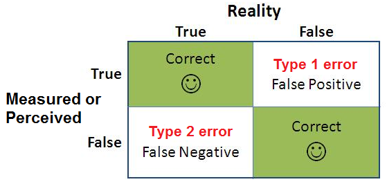
If the result of the test corresponds with reality, then a correct decision has been made. However, if the result of the test does not correspond with reality, then an error has occurred. There are two situations in which the decision is wrong. The null hypothesis may be true, whereas we reject H0. On the other hand, the alternative hypothesis H1 may be true, whereas we do not reject H0. Two types of error are distinguished: type I error and type II error.[3]
Type I error[edit]
The first kind of error is the mistaken rejection of a null hypothesis as the result of a test procedure. This kind of error is called a type I error (false positive) and is sometimes called an error of the first kind. In terms of the courtroom example, a type I error corresponds to convicting an innocent defendant.
Type II error[edit]
The second kind of error is the mistaken failure to reject the null hypothesis as the result of a test procedure. This sort of error is called a type II error (false negative) and is also referred to as an error of the second kind. In terms of the courtroom example, a type II error corresponds to acquitting a criminal.[4]
Crossover error rate[edit]
The crossover error rate (CER) is the point at which type I errors and type II errors are equal. A system with a lower CER value provides more accuracy than a system with a higher CER value.
False positive and false negative[edit]
In terms of false positives and false negatives, a positive result corresponds to rejecting the null hypothesis, while a negative result corresponds to failing to reject the null hypothesis; «false» means the conclusion drawn is incorrect. Thus, a type I error is equivalent to a false positive, and a type II error is equivalent to a false negative.
Table of error types[edit]
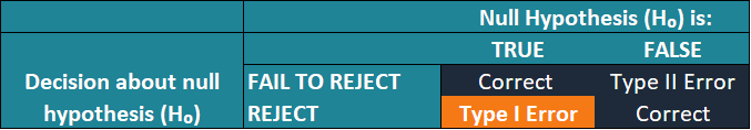
Tabularised relations between truth/falseness of the null hypothesis and outcomes of the test:[5]
| Table of error types | Null hypothesis (H0) is |
||
|---|---|---|---|
| True | False | ||
| Decision about null hypothesis (H0) |
Don’t reject |
Correct inference (true negative) (probability = 1−α) |
Type II error (false negative) (probability = β) |
| Reject | Type I error (false positive) (probability = α) |
Correct inference (true positive) (probability = 1−β) |
Error rate[edit]

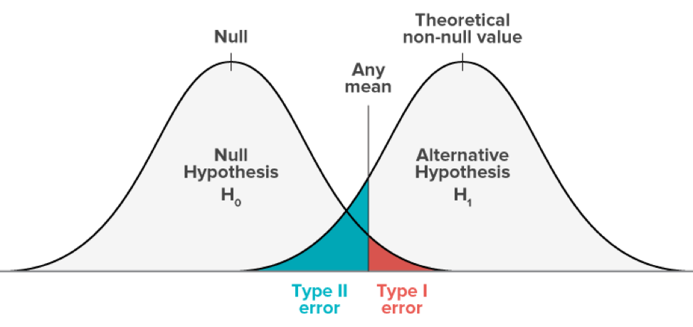
The results obtained from negative sample (left curve) overlap with the results obtained from positive samples (right curve). By moving the result cutoff value (vertical bar), the rate of false positives (FP) can be decreased, at the cost of raising the number of false negatives (FN), or vice versa (TP = True Positives, TPR = True Positive Rate, FPR = False Positive Rate, TN = True Negatives).
A perfect test would have zero false positives and zero false negatives. However, statistical methods are probabilistic, and it cannot be known for certain whether statistical conclusions are correct. Whenever there is uncertainty, there is the possibility of making an error. Considering this nature of statistics science, all statistical hypothesis tests have a probability of making type I and type II errors.[6]
- The type I error rate is the probability of rejecting the null hypothesis given that it is true. The test is designed to keep the type I error rate below a prespecified bound called the significance level, usually denoted by the Greek letter α (alpha) and is also called the alpha level. Usually, the significance level is set to 0.05 (5%), implying that it is acceptable to have a 5% probability of incorrectly rejecting the true null hypothesis.[7]
- The rate of the type II error is denoted by the Greek letter β (beta) and related to the power of a test, which equals 1−β.[8]
These two types of error rates are traded off against each other: for any given sample set, the effort to reduce one type of error generally results in increasing the other type of error.[9]
The quality of hypothesis test[edit]
The same idea can be expressed in terms of the rate of correct results and therefore used to minimize error rates and improve the quality of hypothesis test. To reduce the probability of committing a type I error, making the alpha value more stringent is quite simple and efficient. To decrease the probability of committing a type II error, which is closely associated with analyses’ power, either increasing the test’s sample size or relaxing the alpha level could increase the analyses’ power.[10] A test statistic is robust if the type I error rate is controlled.
Varying different threshold (cut-off) value could also be used to make the test either more specific or more sensitive, which in turn elevates the test quality. For example, imagine a medical test, in which an experimenter might measure the concentration of a certain protein in the blood sample. The experimenter could adjust the threshold (black vertical line in the figure) and people would be diagnosed as having diseases if any number is detected above this certain threshold. According to the image, changing the threshold would result in changes in false positives and false negatives, corresponding to movement on the curve.[11]
Example[edit]
Since in a real experiment it is impossible to avoid all type I and type II errors, it is important to consider the amount of risk one is willing to take to falsely reject H0 or accept H0. The solution to this question would be to report the p-value or significance level α of the statistic. For example, if the p-value of a test statistic result is estimated at 0.0596, then there is a probability of 5.96% that we falsely reject H0. Or, if we say, the statistic is performed at level α, like 0.05, then we allow to falsely reject H0 at 5%. A significance level α of 0.05 is relatively common, but there is no general rule that fits all scenarios.
Vehicle speed measuring[edit]
The speed limit of a freeway in the United States is 120 kilometers per hour. A device is set to measure the speed of passing vehicles. Suppose that the device will conduct three measurements of the speed of a passing vehicle, recording as a random sample X1, X2, X3. The traffic police will or will not fine the drivers depending on the average speed  . That is to say, the test statistic

In addition, we suppose that the measurements X1, X2, X3 are modeled as normal distribution N(μ,4). Then, T should follow N(μ,4/3) and the parameter μ represents the true speed of passing vehicle. In this experiment, the null hypothesis H0 and the alternative hypothesis H1 should be
H0: μ=120 against H1: μ>120.
If we perform the statistic level at α=0.05, then a critical value c should be calculated to solve

According to change-of-units rule for the normal distribution. Referring to Z-table, we can get

Here, the critical region. That is to say, if the recorded speed of a vehicle is greater than critical value 121.9, the driver will be fined. However, there are still 5% of the drivers are falsely fined since the recorded average speed is greater than 121.9 but the true speed does not pass 120, which we say, a type I error.
The type II error corresponds to the case that the true speed of a vehicle is over 120 kilometers per hour but the driver is not fined. For example, if the true speed of a vehicle μ=125, the probability that the driver is not fined can be calculated as

which means, if the true speed of a vehicle is 125, the driver has the probability of 0.36% to avoid the fine when the statistic is performed at level 125 since the recorded average speed is lower than 121.9. If the true speed is closer to 121.9 than 125, then the probability of avoiding the fine will also be higher.
The tradeoffs between type I error and type II error should also be considered. That is, in this case, if the traffic police do not want to falsely fine innocent drivers, the level α can be set to a smaller value, like 0.01. However, if that is the case, more drivers whose true speed is over 120 kilometers per hour, like 125, would be more likely to avoid the fine.
Etymology[edit]
In 1928, Jerzy Neyman (1894–1981) and Egon Pearson (1895–1980), both eminent statisticians, discussed the problems associated with «deciding whether or not a particular sample may be judged as likely to have been randomly drawn from a certain population»:[12] and, as Florence Nightingale David remarked, «it is necessary to remember the adjective ‘random’ [in the term ‘random sample’] should apply to the method of drawing the sample and not to the sample itself».[13]
They identified «two sources of error», namely:
- (a) the error of rejecting a hypothesis that should have not been rejected, and
- (b) the error of failing to reject a hypothesis that should have been rejected.
In 1930, they elaborated on these two sources of error, remarking that:
…in testing hypotheses two considerations must be kept in view, we must be able to reduce the chance of rejecting a true hypothesis to as low a value as desired; the test must be so devised that it will reject the hypothesis tested when it is likely to be false.
In 1933, they observed that these «problems are rarely presented in such a form that we can discriminate with certainty between the true and false hypothesis» . They also noted that, in deciding whether to fail to reject, or reject a particular hypothesis amongst a «set of alternative hypotheses», H1, H2…, it was easy to make an error:
…[and] these errors will be of two kinds:
- (I) we reject H0 [i.e., the hypothesis to be tested] when it is true,[14]
- (II) we fail to reject H0 when some alternative hypothesis HA or H1 is true. (There are various notations for the alternative).
In all of the papers co-written by Neyman and Pearson the expression H0 always signifies «the hypothesis to be tested».
In the same paper they call these two sources of error, errors of type I and errors of type II respectively.[15]
[edit]
Null hypothesis[edit]
It is standard practice for statisticians to conduct tests in order to determine whether or not a «speculative hypothesis» concerning the observed phenomena of the world (or its inhabitants) can be supported. The results of such testing determine whether a particular set of results agrees reasonably (or does not agree) with the speculated hypothesis.
On the basis that it is always assumed, by statistical convention, that the speculated hypothesis is wrong, and the so-called «null hypothesis» that the observed phenomena simply occur by chance (and that, as a consequence, the speculated agent has no effect) – the test will determine whether this hypothesis is right or wrong. This is why the hypothesis under test is often called the null hypothesis (most likely, coined by Fisher (1935, p. 19)), because it is this hypothesis that is to be either nullified or not nullified by the test. When the null hypothesis is nullified, it is possible to conclude that data support the «alternative hypothesis» (which is the original speculated one).
The consistent application by statisticians of Neyman and Pearson’s convention of representing «the hypothesis to be tested» (or «the hypothesis to be nullified») with the expression H0 has led to circumstances where many understand the term «the null hypothesis» as meaning «the nil hypothesis» – a statement that the results in question have arisen through chance. This is not necessarily the case – the key restriction, as per Fisher (1966), is that «the null hypothesis must be exact, that is free from vagueness and ambiguity, because it must supply the basis of the ‘problem of distribution,’ of which the test of significance is the solution.»[16] As a consequence of this, in experimental science the null hypothesis is generally a statement that a particular treatment has no effect; in observational science, it is that there is no difference between the value of a particular measured variable, and that of an experimental prediction.[citation needed]
Statistical significance[edit]
If the probability of obtaining a result as extreme as the one obtained, supposing that the null hypothesis were true, is lower than a pre-specified cut-off probability (for example, 5%), then the result is said to be statistically significant and the null hypothesis is rejected.
British statistician Sir Ronald Aylmer Fisher (1890–1962) stressed that the «null hypothesis»:
… is never proved or established, but is possibly disproved, in the course of experimentation. Every experiment may be said to exist only in order to give the facts a chance of disproving the null hypothesis.
— Fisher, 1935, p.19
Application domains[edit]
Medicine[edit]
In the practice of medicine, the differences between the applications of screening and testing are considerable.
Medical screening[edit]
Screening involves relatively cheap tests that are given to large populations, none of whom manifest any clinical indication of disease (e.g., Pap smears).
Testing involves far more expensive, often invasive, procedures that are given only to those who manifest some clinical indication of disease, and are most often applied to confirm a suspected diagnosis.
For example, most states in the USA require newborns to be screened for phenylketonuria and hypothyroidism, among other congenital disorders.
Hypothesis: «The newborns have phenylketonuria and hypothyroidism»
Null Hypothesis (H0): «The newborns do not have phenylketonuria and hypothyroidism»,
Type I error (false positive): The true fact is that the newborns do not have phenylketonuria and hypothyroidism but we consider they have the disorders according to the data.
Type II error (false negative): The true fact is that the newborns have phenylketonuria and hypothyroidism but we consider they do not have the disorders according to the data.
Although they display a high rate of false positives, the screening tests are considered valuable because they greatly increase the likelihood of detecting these disorders at a far earlier stage.
The simple blood tests used to screen possible blood donors for HIV and hepatitis have a significant rate of false positives; however, physicians use much more expensive and far more precise tests to determine whether a person is actually infected with either of these viruses.
Perhaps the most widely discussed false positives in medical screening come from the breast cancer screening procedure mammography. The US rate of false positive mammograms is up to 15%, the highest in world. One consequence of the high false positive rate in the US is that, in any 10-year period, half of the American women screened receive a false positive mammogram. False positive mammograms are costly, with over $100 million spent annually in the U.S. on follow-up testing and treatment. They also cause women unneeded anxiety. As a result of the high false positive rate in the US, as many as 90–95% of women who get a positive mammogram do not have the condition. The lowest rate in the world is in the Netherlands, 1%. The lowest rates are generally in Northern Europe where mammography films are read twice and a high threshold for additional testing is set (the high threshold decreases the power of the test).
The ideal population screening test would be cheap, easy to administer, and produce zero false-negatives, if possible. Such tests usually produce more false-positives, which can subsequently be sorted out by more sophisticated (and expensive) testing.
Medical testing[edit]
False negatives and false positives are significant issues in medical testing.
Hypothesis: «The patients have the specific disease».
Null hypothesis (H0): «The patients do not have the specific disease».
Type I error (false positive): «The true fact is that the patients do not have a specific disease but the physicians judges the patients was ill according to the test reports».
False positives can also produce serious and counter-intuitive problems when the condition being searched for is rare, as in screening. If a test has a false positive rate of one in ten thousand, but only one in a million samples (or people) is a true positive, most of the positives detected by that test will be false. The probability that an observed positive result is a false positive may be calculated using Bayes’ theorem.
Type II error (false negative): «The true fact is that the disease is actually present but the test reports provide a falsely reassuring message to patients and physicians that the disease is absent».
False negatives produce serious and counter-intuitive problems, especially when the condition being searched for is common. If a test with a false negative rate of only 10% is used to test a population with a true occurrence rate of 70%, many of the negatives detected by the test will be false.
This sometimes leads to inappropriate or inadequate treatment of both the patient and their disease. A common example is relying on cardiac stress tests to detect coronary atherosclerosis, even though cardiac stress tests are known to only detect limitations of coronary artery blood flow due to advanced stenosis.
Biometrics[edit]
Biometric matching, such as for fingerprint recognition, facial recognition or iris recognition, is susceptible to type I and type II errors.
Hypothesis: «The input does not identify someone in the searched list of people»
Null hypothesis: «The input does identify someone in the searched list of people»
Type I error (false reject rate): «The true fact is that the person is someone in the searched list but the system concludes that the person is not according to the data».
Type II error (false match rate): «The true fact is that the person is not someone in the searched list but the system concludes that the person is someone whom we are looking for according to the data».
The probability of type I errors is called the «false reject rate» (FRR) or false non-match rate (FNMR), while the probability of type II errors is called the «false accept rate» (FAR) or false match rate (FMR).
If the system is designed to rarely match suspects then the probability of type II errors can be called the «false alarm rate». On the other hand, if the system is used for validation (and acceptance is the norm) then the FAR is a measure of system security, while the FRR measures user inconvenience level.
Security screening[edit]
False positives are routinely found every day in airport security screening, which are ultimately visual inspection systems. The installed security alarms are intended to prevent weapons being brought onto aircraft; yet they are often set to such high sensitivity that they alarm many times a day for minor items, such as keys, belt buckles, loose change, mobile phones, and tacks in shoes.
Here, the null hypothesis is that the item is not a weapon, while the alternative hypothesis is that the item is a weapon.
A type I error (false positive): «The true fact is that the item is not a weapon but the system still alarms».
Type II error (false negative) «The true fact is that the item is a weapon but the system keeps silent at this time».
The ratio of false positives (identifying an innocent traveler as a terrorist) to true positives (detecting a would-be terrorist) is, therefore, very high; and because almost every alarm is a false positive, the positive predictive value of these screening tests is very low.
The relative cost of false results determines the likelihood that test creators allow these events to occur. As the cost of a false negative in this scenario is extremely high (not detecting a bomb being brought onto a plane could result in hundreds of deaths) whilst the cost of a false positive is relatively low (a reasonably simple further inspection) the most appropriate test is one with a low statistical specificity but high statistical sensitivity (one that allows a high rate of false positives in return for minimal false negatives).
Computers[edit]
The notions of false positives and false negatives have a wide currency in the realm of computers and computer applications, including computer security, spam filtering, Malware, Optical character recognition and many others.
For example, in the case of spam filtering the hypothesis here is that the message is a spam.
Thus, null hypothesis: «The message is not a spam».
Type I error (false positive): «Spam filtering or spam blocking techniques wrongly classify a legitimate email message as spam and, as a result, interferes with its delivery».
While most anti-spam tactics can block or filter a high percentage of unwanted emails, doing so without creating significant false-positive results is a much more demanding task.
Type II error (false negative): «Spam email is not detected as spam, but is classified as non-spam». A low number of false negatives is an indicator of the efficiency of spam filtering.
See also[edit]
- Binary classification
- Detection theory
- Egon Pearson
- Ethics in mathematics
- False positive paradox
- False discovery rate
- Family-wise error rate
- Information retrieval performance measures
- Neyman–Pearson lemma
- Null hypothesis
- Probability of a hypothesis for Bayesian inference
- Precision and recall
- Prosecutor’s fallacy
- Prozone phenomenon
- Receiver operating characteristic
- Sensitivity and specificity
- Statisticians’ and engineers’ cross-reference of statistical terms
- Testing hypotheses suggested by the data
- Type III error
References[edit]
- ^ «Type I Error and Type II Error». explorable.com. Retrieved 14 December 2019.
- ^ Chow, Y. W.; Pietranico, R.; Mukerji, A. (27 October 1975). «Studies of oxygen binding energy to hemoglobin molecule». Biochemical and Biophysical Research Communications. 66 (4): 1424–1431. doi:10.1016/0006-291x(75)90518-5. ISSN 0006-291X. PMID 6.
- ^ A modern introduction to probability and statistics : understanding why and how. Dekking, Michel, 1946-. London: Springer. 2005. ISBN 978-1-85233-896-1. OCLC 262680588.
{{cite book}}: CS1 maint: others (link) - ^ A modern introduction to probability and statistics : understanding why and how. Dekking, Michel, 1946-. London: Springer. 2005. ISBN 978-1-85233-896-1. OCLC 262680588.
{{cite book}}: CS1 maint: others (link) - ^ Sheskin, David (2004). Handbook of Parametric and Nonparametric Statistical Procedures. CRC Press. p. 54. ISBN 1584884401.
- ^ Smith, R. J.; Bryant, R. G. (27 October 1975). «Metal substitutions incarbonic anhydrase: a halide ion probe study». Biochemical and Biophysical Research Communications. 66 (4): 1281–1286. doi:10.1016/0006-291x(75)90498-2. ISSN 0006-291X. PMC 9650581. PMID 3.
- ^ Lindenmayer, David. (2005). Practical conservation biology. Burgman, Mark A. Collingwood, Vic.: CSIRO Pub. ISBN 0-643-09310-9. OCLC 65216357.
- ^ Chow, Y. W.; Pietranico, R.; Mukerji, A. (27 October 1975). «Studies of oxygen binding energy to hemoglobin molecule». Biochemical and Biophysical Research Communications. 66 (4): 1424–1431. doi:10.1016/0006-291x(75)90518-5. ISSN 0006-291X. PMID 6.
- ^ Smith, R. J.; Bryant, R. G. (27 October 1975). «Metal substitutions incarbonic anhydrase: a halide ion probe study». Biochemical and Biophysical Research Communications. 66 (4): 1281–1286. doi:10.1016/0006-291x(75)90498-2. ISSN 0006-291X. PMC 9650581. PMID 3.
- ^ Smith, R. J.; Bryant, R. G. (27 October 1975). «Metal substitutions incarbonic anhydrase: a halide ion probe study». Biochemical and Biophysical Research Communications. 66 (4): 1281–1286. doi:10.1016/0006-291x(75)90498-2. ISSN 0006-291X. PMC 9650581. PMID 3.
- ^ Moroi, K.; Sato, T. (15 August 1975). «Comparison between procaine and isocarboxazid metabolism in vitro by a liver microsomal amidase-esterase». Biochemical Pharmacology. 24 (16): 1517–1521. doi:10.1016/0006-2952(75)90029-5. ISSN 1873-2968. PMID 8.
- ^ NEYMAN, J.; PEARSON, E. S. (1928). «On the Use and Interpretation of Certain Test Criteria for Purposes of Statistical Inference Part I». Biometrika. 20A (1–2): 175–240. doi:10.1093/biomet/20a.1-2.175. ISSN 0006-3444.
- ^ C.I.K.F. (July 1951). «Probability Theory for Statistical Methods. By F. N. David. [Pp. ix + 230. Cambridge University Press. 1949. Price 155.]». Journal of the Staple Inn Actuarial Society. 10 (3): 243–244. doi:10.1017/s0020269x00004564. ISSN 0020-269X.
- ^ Note that the subscript in the expression H0 is a zero (indicating null), and is not an «O» (indicating original).
- ^ Neyman, J.; Pearson, E. S. (30 October 1933). «The testing of statistical hypotheses in relation to probabilities a priori». Mathematical Proceedings of the Cambridge Philosophical Society. 29 (4): 492–510. Bibcode:1933PCPS…29..492N. doi:10.1017/s030500410001152x. ISSN 0305-0041. S2CID 119855116.
- ^ Fisher, R.A. (1966). The design of experiments. 8th edition. Hafner:Edinburgh.
Bibliography[edit]
- Betz, M.A. & Gabriel, K.R., «Type IV Errors and Analysis of Simple Effects», Journal of Educational Statistics, Vol.3, No.2, (Summer 1978), pp. 121–144.
- David, F.N., «A Power Function for Tests of Randomness in a Sequence of Alternatives», Biometrika, Vol.34, Nos.3/4, (December 1947), pp. 335–339.
- Fisher, R.A., The Design of Experiments, Oliver & Boyd (Edinburgh), 1935.
- Gambrill, W., «False Positives on Newborns’ Disease Tests Worry Parents», Health Day, (5 June 2006). [1] Archived 17 May 2018 at the Wayback Machine
- Kaiser, H.F., «Directional Statistical Decisions», Psychological Review, Vol.67, No.3, (May 1960), pp. 160–167.
- Kimball, A.W., «Errors of the Third Kind in Statistical Consulting», Journal of the American Statistical Association, Vol.52, No.278, (June 1957), pp. 133–142.
- Lubin, A., «The Interpretation of Significant Interaction», Educational and Psychological Measurement, Vol.21, No.4, (Winter 1961), pp. 807–817.
- Marascuilo, L.A. & Levin, J.R., «Appropriate Post Hoc Comparisons for Interaction and nested Hypotheses in Analysis of Variance Designs: The Elimination of Type-IV Errors», American Educational Research Journal, Vol.7., No.3, (May 1970), pp. 397–421.
- Mitroff, I.I. & Featheringham, T.R., «On Systemic Problem Solving and the Error of the Third Kind», Behavioral Science, Vol.19, No.6, (November 1974), pp. 383–393.
- Mosteller, F., «A k-Sample Slippage Test for an Extreme Population», The Annals of Mathematical Statistics, Vol.19, No.1, (March 1948), pp. 58–65.
- Moulton, R.T., «Network Security», Datamation, Vol.29, No.7, (July 1983), pp. 121–127.
- Raiffa, H., Decision Analysis: Introductory Lectures on Choices Under Uncertainty, Addison–Wesley, (Reading), 1968.
External links[edit]
- Bias and Confounding – presentation by Nigel Paneth, Graduate School of Public Health, University of Pittsburgh
Learn / Guides / CRO glossary
Back to guides
CRO glossary: type 1 error
What is a type 1 error?
Type 1 error is a term statisticians use to describe a false positive—a test result that incorrectly affirms a false statement about the nature of reality.
Best practices: marketers and product or website owners
In A/B testing, type 1 errors occur when experimenters falsely conclude that any variation of an A/B or multivariate test outperformed the other(s) due to something more than random chance. Type 1 errors can hurt conversions when companies make website changes based on incorrect information.
Type 1 errors vs. type 2 errors
While a type 1 error implies a false positive—that one version outperforms another—a type 2 error implies a false negative. In other words, a type 2 error falsely concludes that there is no statistically significant difference between conversion rates of different variations when there actually is a difference.
Here’s what that looks like:

What causes type 1 errors?
Type 1 errors can result from two sources: random chance and improper research techniques.
Random chance: no random sample, whether it’s a pre-election poll or an A/B test, can ever perfectly represent the population it intends to describe. Since researchers sample a small portion of the total population, it’s possible that the results don’t accurately predict or represent reality—that the conclusions are the product of random chance.
Statistical significance measures the odds that the results of an A/B test were produced by random chance. For example, let’s say you’ve run an A/B test that shows Version B outperforming Version A with a statistical significance of 95%. That means there’s a 5% chance these results were produced by random chance.You can raise your level of statistical significance by increasing the sample size, but this requires more traffic and therefore takes more time. In the end, you have to strike a balance between your desired level of accuracy and the resources you have available.
Improper research techniques: when running an A/B test, it’s important to gather enough data to reach your desired level of statistical significance. Sloppy researchers might start running a test and pull the plug when they feel there’s a ‘clear winner’—long before they’ve gathered enough data to reach their desired level of statistical significance. There’s really no excuse for a type 1 error like this.
Why are type 1 errors important?
Type 1 errors can have a huge impact on conversions. For example, if you A/B test two page versions and incorrectly conclude that version B is the winner, you could see a massive drop in conversions when you take that change live for all your visitors to see. As mentioned above, this could be the result of poor experimentation techniques, but it might also be the result of random chance. Type 1 errors can (and do) result from flawless experimentation.
When you make a change to a webpage based on A/B testing, it’s important to understand that you may be working with incorrect conclusions produced by type 1 errors.
Understanding type 1 errors allows you to:
-
Choose the level of risk you’re willing to accept (e.g., increase your sample size to achieve a higher level of statistical significance)
-
Do proper experimentation to reduce your risk of human-caused type 1 errors
-
Recognize when a type 1 error may have caused a drop in conversions so you can fix the problem
It’s impossible to achieve 100% statistical significance (and it’s usually impractical to aim for 99% statistical significance, since it requires a disproportionately large sample size compared to 95%-97% statistical significance). The goal of CRO isn’t to get it right every time—it’s to make the right choices most of the time. And when you understand type 1 errors, you increase your odds of getting it right.
How do you minimize type 1 errors?
The only way to minimize type 1 errors, assuming you’re A/B testing properly, is to raise your level of statistical significance. Of course, if you want a higher level of statistical significance, you’ll need a larger sample size.
It isn’t a challenge to study large sample sizes if you’ve got massive amounts of traffic, but if your website doesn’t generate that level of traffic, you’ll need to be more selective about what you decide to study—especially if you’re going for higher statistical significance.
Here’s how to narrow down the focus of your experiments.
6 ways to find the most important elements to test
In order to test what matters most, you need to determine what really matters to your target audience. Here are six ways to figure out what’s worth testing.
-
Read reviews and speak with your Customer Support department: figure out what people think of your brand and products. Talk to Sales, Customer Support, and Product Design to get a sense of what people really want from you and your products.
-
Figure out why visitors leave without buying: traditional analytics tools (e.g., Google Analytics) can show where people leave the site. Combining this data with Hotjar’s Conversion Funnels Tool will give you a strong sense of which pages are worth focusing on.
-
Discover the page elements that people engage: heatmaps show where the majority of users click, scroll, and hover their mouse pointers (or tap their fingers on mobile devices and tablets).
Heatmaps will help you find trends in how visitors interact with key pages on your website, which in turn will help you decide which elements to keep (since they work) and which ones are being ignored and need further examination. -
Gather feedback from customers: on-page surveys, polls, and feedback widgets give your customers a way to quickly send feedback about their experience your way. This will alert you to issues you never knew existed and will help you prioritize what needs fixing for the experience to improve.
-
Look at session recordings: see how individual (anonymized) users behave on your site. Notice where they struggle and how they go back and forth when they can’t find what they need. Pro tip: pay particular attention to what they do just before they leave your site.
-
Explore usability testing: can help you understand how people see and experience your website. Capture spoken feedback about issues they encounter, and discover what could improve their experience.
Pro tip: do you want to improve everyone’s experience? That may be tempting, but you’ll get a whole lot further by focusing on your ideal customers. To learn more about identifying your ideal customers, check out our blog post about creating simple user personas.
A type I error is a kind of fault that occurs during the hypothesis testing process when a null hypothesis is rejected, even though it is accurate and should not be rejected.
In hypothesis testing, a null hypothesis is established before the onset of a test. In some cases, the null hypothesis assumes that there’s no cause and effect relationship between the item being tested and the stimuli being applied to the test subject to trigger an outcome to the test.
However, errors can occur whereby the null hypothesis has been rejected, meaning it’s determined there is a cause and effect relationship between the testing variables when, in reality, it’s a false positive. These false positives are called type I errors.
Key Takeaways
- A type I error occurs during hypothesis testing when a null hypothesis is rejected, even though it is accurate and should not be rejected.
- The null hypothesis assumes no cause and effect relationship between the tested item and the stimuli applied during the test.
- A type I error is a «false positive» leading to an incorrect rejection of the null hypothesis.
Understanding a Type I Error
Hypothesis testing is a process of testing a conjecture by using sample data. The test is designed to provide evidence that the conjecture or hypothesis is supported by the data being tested. A null hypothesis is the belief that there is no statistical significance or effect between the two data sets, variables, or populations being considered in the hypothesis. Typically, a researcher would try to disprove the null hypothesis.
For example, let’s say the null hypothesis states that an investment strategy doesn’t perform any better than a market index, such as the S&P 500. The researcher would take samples of data and test the historical performance of the investment strategy to determine if the strategy performed at a higher level than the S&P. If the test results showed that the strategy performed at a higher rate than the index, the null hypothesis would be rejected.
This condition is denoted as «n=0.» If—when the test is conducted—the result seems to indicate that the stimuli applied to the test subject caused a reaction, the null hypothesis stating that the stimuli do not affect the test subject would, in turn, need to be rejected.
Ideally, a null hypothesis should never be rejected if it’s found to be true, and it should always be rejected if it’s found to be false. However, there are situations when errors can occur.
False Positive Type I Error
Sometimes, rejecting the null hypothesis that there is no relationship between the test subject, the stimuli, and the outcome can be incorrect. If something other than the stimuli causes the outcome of the test, it can cause a «false positive» result where it appears the stimuli acted upon the subject, but the outcome was caused by chance. This «false positive,» leading to an incorrect rejection of the null hypothesis, is called a type I error. A type I error rejects an idea that should not have been rejected.
Examples of Type I Errors
For example, let’s look at the trial of an accused criminal. The null hypothesis is that the person is innocent, while the alternative is guilty. A type I error in this case would mean that the person is not found innocent and is sent to jail, despite actually being innocent.
In medical testing, a type I error would cause the appearance that a treatment for a disease has the effect of reducing the severity of the disease when, in fact, it does not. When a new medicine is being tested, the null hypothesis will be that the medicine does not affect the progression of the disease. Let’s say a lab is researching a new cancer drug. Their null hypothesis might be that the drug does not affect the growth rate of cancer cells.
After applying the drug to the cancer cells, the cancer cells stop growing. This would cause the researchers to reject their null hypothesis that the drug would have no effect. If the drug caused the growth stoppage, the conclusion to reject the null, in this case, would be correct. However, if something else during the test caused the growth stoppage instead of the administered drug, this would be an example of an incorrect rejection of the null hypothesis (i.e., a type I error).
There are two common types of errors, type I and type II errors you’ll likely encounter when testing a statistical hypothesis. The mistaken rejection of the finding or the null hypothesis is known as a type I error. In other words, type I error is the false-positive finding in hypothesis testing. Type II error on the other hand is the false-negative finding in hypothesis testing.
To better understand the two types of errors, here’s an example:
Let’s assume you notice some flu-like symptoms and decide to go to a hospital to get tested for the presence of malaria. There is a possibility of two errors occurring:
- In type I error (False positive): The result of the test shows you have malaria but you actually don’t have it.
- Type II error (false negative): The test result indicates that you don’t have malaria when you in fact do.
Type I error and Type II error are extensively used in areas such as computer science, Engineering, Statistics, and many more.
The chance of committing a type I error is known as alpha (α), while the chance of committing a type II error is known as beta (β). If you carefully plan your study design, you can minimize the probability of committing either of the errors.
Read: Survey Errors To Avoid: Types, Sources, Examples, Mitigation
What are Type I Errors?
Type I error is an omission that happens when a null hypothesis is reprobated during hypothesis testing. This is when it is indeed precise or positive and should not have been initially disapproved. So if a null hypothesis is erroneously rejected when it is positive, it is called a Type I error.
What this means is that results are concluded to be significant when in actual fact, it was obtained by chance.
When conducting hypothesis testing, a null hypothesis is determined before carrying out the actual test. The null hypothesis may presume that there is no chain of circumstances between the items being tested which may cause an outcome for the test.
When a null hypothesis is rejected, it means a chain of circumstances has been established between the items being tested even though it is a false alarm or false positive. This could lead to an error or many errors in a test, known as a Type I error.
It is worthy of note that statistical outcomes of every testing involve uncertainties, so making errors while performing these hypothesis testings is unavoidable. It is inherent that type I error may be considered as an error of commission in the sense that the producer or researcher mistakenly decides on a false outcome.
Read: Systematic Errors in Research: Definition, Examples
Causes of Type I Error
- When a factor other than the variable affects the variables being tested. This factor that causes the effect produces a result that supports the decision to reject the null hypothesis.
- When the result of a hypothesis testing is caused by chance, it is a Type I error.
- Lastly, because a null hypothesis and the significance level are decided before conducting a hypothesis test, and also the sample size is not considered, a type I error may occur due to chance.
Read: Margin of error – Definition, Formula + Application
Risk Factor and Probability of Type I Error
- The risk factor and probability of Type I error are mostly set in advance and the level of significance of the hypothesis testing is known.
- The level of significance in a test is represented by α and it signifies the rate of the possibility of Type I error.
- While it is possible to reduce the rate of Type I error by using a determined sample size. The consequence of this, however, is that the possibility of a Type II error occurring in a test will increase.
- In a case where Type I error is decided at 5 percent, it means in the null hypothesis (H0), chances are there that 5 in the 100 hypotheses even if true will be rejected.
- Another risk factor is that both Type I and Type II errors can not be changed simultaneously. To reduce the possibility of one error occurring means the possibility of the other error will increase. Hence changing the outcome of one test inherently affects the outcome of the other test.
Read: Sampling Bias: Definition, Types + [Examples]
Consequences of a Type I Error
A type I error will result in a false alarm. The outcome of the hypothesis testing will be a false positive. This implies that the researcher decided the result of a hypothesis testing is true when in fact, it is not.
For a sales group, the consequences of a type I error may result in losing potential market and missing out on probable sales because the findings of a test are faulty.
What are Type II Errors?
A Type II error means a researcher or producer did not disapprove of the alternate hypothesis when it is in fact negative or false. This does not mean the null hypothesis is accepted as positive as hypothesis testing only indicates if a null hypothesis should be rejected.
A Type II error means a conclusion on the effect of the test wasn’t recognized when an effect truly existed. Before a test can be said to have a real effect, it has to have a power level that is 80% or more.
This implies the statistical power of a test determines the risk of a type II error. The probability of a type II error occurring largely depends on how high the statistical power is.
Note: Null hypothesis is represented as (H0) and alternative hypothesis is represented as (H1)
Causes of Type II Error
- Type II error is mainly caused by the statistical power of a test being low. A Type II error will occur if the statistical test is not powerful enough.
- The size of the sample can also lead to a Type I error because the outcome of the test will be affected. A small sample size might hide the significant level of the items being tested.
- Another cause of Type Ii error is the possibility that a researcher may disapprove of the actual outcome of a hypothesis even when it is correct.
Probability of Type II Error
- To arrive at the possibility of a Type II error occurring, the power of the test must be deducted from type 1.
- The level of significance in a test is represented by β and it shows the rate of the possibility of Type I error.
- It is possible to reduce the rate of Type II error if the significance level of the test is increased.
- In a case where Type II error is decided at 5 percent, it means in the null hypothesis (H0), chances are there that 5 in the 100 hypotheses even if it is false will be accepted.
- Type I error and Type II error are connected. Hence, to reduce the possibility of one type of error from occurring means the possibility of the other error will increase.
- It is important to decide which error has lesser effects on the test.
Consequences of a Type II Error
Type II errors can also result in a wrong decision that will affect the outcomes of a test and have real-life consequences.
Note that even if you proved your test hypothesis, your conversion result can invalidate the outcome unintended. This turn of events can be discouraging, hence the need to be extra careful when conducting hypothesis testing.
How to Avoid Type I and II errors
Type I error and type II errors can not be entirely avoided in hypothesis testing, but the researcher can reduce the probability of them occurring.
For Type I error, minimize the significance level to avoid making errors. This can be determined by the researcher.
To avoid type II errors, ensure the test has high statistical power. The higher the statistical power, the higher the chance of avoiding an error. Set your statistical power to 80% and above and conduct your test.
Increase the sample size of the hypothesis testing.
The Type II error can also be avoided if the significance level of the test hypothesis is chosen.
How to Detect Type I and Type II Errors in Data
After completing a study, the researcher can conduct any of the available statistical tests to reject the default hypothesis in favor of its alternative. If the study is free of bias, there are four possible outcomes. See the image below;
Image source: IPJ
If the findings in the sample and reality in the population match, the researchers’ inferences will be correct. However, if in any of the situations a type I or II error has been made, the inference will be incorrect.
Key Differences between Type I & II Errors
- In statistical hypothesis testing, a type I error is caused by disapproving a null hypothesis that is otherwise correct while in contrast, Type II error occurs when the null hypothesis is not rejected even though it is not true.
- Type I error is the same as a false alarm or false positive while Type II error is also referred to as false negative.
- A Type I error is represented by α while a Type II error is represented by β.
- The level of significance determines the possibility of a type I error while type II error is the possibility of deducting the power of the test from 1.
- You can decrease the possibility of Type I error by reducing the level of significance. The same way you can reduce the probability of a Type II error by increasing the significance level of the test.
- Type I error occurs when you reject the null hypothesis, in contrast, Type II error occurs when you accept an incorrect outcome of a false hypothesis
Examples of Type I & II errors
Type I error examples
To understand the statistical significance of Type I error, let us look at this example.
In this hypothesis, a driver wants to determine the relationship between him getting a new driving wheel and the number of passengers he carries in a week.
Now, if the number of passengers he carries in a week increases after he got a new driving wheel than the number of passengers he carried in a week with the old driving wheel, this driver might assume that there is a relationship between the new wheel and the increase in the number of passengers and support the alternative hypothesis.
However, the increment in the number of passengers he carried in a week, might have been influenced by chance and not by the new wheel which results in type I error.
By this indication, the driver should have supported the null hypothesis because the increment of his passengers might have been due to chance and not fact.
Type II error examples
For Type II error and statistical power, let us assume a hypothesis where a farmer that rears birds assumes none of his birds have bird-flu. He observes his birds for four days to find out if there are symptoms of the flu.
If after four days, the farmer sees no symptoms of the flu in his birds, he might assume his birds are indeed free from bird flu whereas the bird flu might have affected his birds and the symptoms are obvious on the sixth day.
By this indication, the farmer accepts that no flu exists in his birds. This leads to a type II error where it supports the null hypothesis when it is in fact false.
Frequently Asked Questions about Type I and II Errors
- Is a Type I or Type II error worse?
Both Type I and type II errors could be worse based on the type of research being conducted.
A Type I error means an incorrect assumption has been made when the assumption is in reality not true. The consequence of this is that other alternatives are disapproved of to accept this conclusion. A type II error implies that a null hypothesis was not rejected. This means that a significant outcome wouldn’t have any benefit in reality.
A Type I error however may be terrible for statisticians. It is difficult to decide which of the errors is worse than the other but both types of errors could do enough damage to your research.
- Does sample size affect type 1 error?
Small or large sample size does not affect type I error. So sample size will not increase the occurrence of Type I error.
The only principle is that your test has a normal sample size. If the sample size is small in Type II errors, the level of significance will decrease.
This may cause a false assumption from the researcher and discredit the outcome of the hypothesis testing.
- What is statistical power as it relates to Type I or Type II errors
Statistical power is used in type II to deduce the measurement error. This is because random errors reduce the statistical power of hypothesis testing. Not only that, the larger the size of the effect, the more detectable the errors are.
The statistical power of a hypothesis increases when the level of significance increases. The statistical power also increases when a larger sample size is being tested thereby reducing the errors. If you want the risk of Type II error to reduce, increase the level of significance of the test.
- What is statistical significance as it relates to Type I or Type II errors
Statistical significance relates to Type I error. Researchers sometimes assume that the outcome of a test is statistically significant when they are not and the researcher then rejects the null hypothesis. The fact is, the outcome might have happened due to chance.
A type I error decreases when a lower significance level is set.
If your test power is lower compared to the significance level, then the alternative hypothesis is relevant to the statistical significance of your test, then the outcome is relevant.
Conclusion
In this article, we have extensively discussed Type I error and Type II error. We have also discussed their causes, the probabilities of their occurrence, and how to avoid them. We have seen that both Types of errors have their usefulness and limitations. The best approach as a researcher is to know which to apply and when.
Statistical hypothesis testing implies that no test is ever 100% certain: that’s because we rely on probabilities to experiment.
When online marketers and scientists run hypothesis tests, they’re both looking for statistically relevant results. This means that the results of their tests have to be true within a range of probabilities (typically 95%).
Even though hypothesis tests are meant to be reliable, there are two types of errors that can still occur.
These errors are known as type 1 and type 2 errors (or type i and type ii errors).
Let’s dive in and understand what type 1 and type 2 errors are and the difference between the two.
Understanding Type I Errors
Type 1 errors – often assimilated with false positives – happen in hypothesis testing when the null hypothesis is true but rejected. The null hypothesis is a general statement or default position that there is no relationship between two measured phenomena.
Simply put, type 1 errors are “false positives” – they happen when the tester validates a statistically significant difference even though there isn’t one.
Type 1 errors have a probability of “α” correlated to the level of confidence that you set. A test with a 95% confidence level means that there is a 5% chance of getting a type 1 error.
Consequences of a Type 1 Error
Why do type 1 errors occur? Type 1 errors can happen due to bad luck (the 5% chance has played against you) or because you didn’t respect the test duration and sample size initially set for your experiment.
Consequently, a type 1 error will bring in a false positive. This means that you will wrongfully assume that your hypothesis testing has worked even though it hasn’t.
In real-life situations, this could potentially mean losing possible sales due to a faulty assumption caused by the test.
Related: Sample Size Calculator for A/B Testing
A Real-Life Example of a Type 1 Error
Let’s say that you want to increase conversions on a banner displayed on your website. For that to work out, you’ve planned on adding an image to see if it increases conversions or not.
You start your A/B test by running a control version (A) against your variation (B) that contains the image. After 5 days, variation (B) outperforms the control version by a staggering 25% increase in conversions with an 85% level of confidence.
You stop the test and implement the image in your banner. However, after a month, you noticed that your month-to-month conversions have actually decreased.
That’s because you’ve encountered a type 1 error: your variation didn’t actually beat your control version in the long run.
Related: Frequentist vs Bayesian Methods in A/B Testing
Want to avoid these types of errors during your digital experiments?
AB Tasty is an a/b testing tool embedded with AI and automation that allows you to quickly set up experiments, track insights via our dashboard, and determine which route will increase your revenue.
Understanding Type II Errors
In the same way that type 1 errors are commonly referred to as “false positives”, type 2 errors are referred to as “false negatives”.
Type 2 errors happen when you inaccurately assume that no winner has been declared between a control version and a variation although there actually is a winner.
In more statistically accurate terms, type 2 errors happen when the null hypothesis is false and you subsequently fail to reject it.
If the probability of making a type 1 error is determined by “α”, the probability of a type 2 error is “β”. Beta depends on the power of the test (i.e the probability of not committing a type 2 error, which is equal to 1-β).
There are 3 parameters that can affect the power of a test:
- Your sample size (n)
- The significance level of your test (α)
- The “true” value of your tested parameter (read more here)
Consequences of a Type 2 Error
Similarly to type 1 errors, type 2 errors can lead to false assumptions and poor decision-making that can result in lost sales or decreased profits.
Moreover, getting a false negative (without realizing it) can discredit your conversion optimization efforts even though you could have proven your hypothesis. This can be a discouraging turn of events that could happen to any CRO expert and/or digital marketer.
A Real-Life Example of a Type 2 Error
Let’s say that you run an e-commerce store that sells cosmetic products for consumers. In an attempt to increase conversions, you have the idea to implement social proof messaging on your product pages, like NYX Professional Makeup.
 You launch an A/B test to see if the variation (B) could outperform your control version (A).
After a week, you do not notice any difference in conversions: both versions seem to convert at the same rate and you start questioning your assumption. Three days later, you stop the test and keep your product page as it is.
At this point, you assume that adding social proof messaging to your store didn’t have any effect on conversions.
Two weeks later, you hear that a competitor had added social proof messages at the same time and observed tangible gains in conversions. You decide to re-run the test for a month in order to get more statistically relevant results based on an increased level of confidence (say 95%).
After a month – surprise – you discover positive gains in conversions for the variation (B). Adding social proof messages under the purchase buttons on your product pages has indeed brought your company more sales than the control version.
That’s right – your first test encountered a type 2 error!
Why are Type I and Type II Errors Important?
Type one and type two errors are errors that we may encounter on a daily basis. It’s important to understand these errors and the impact that they can have on your daily life.
With type 1 errors you are making an incorrect assumption and can lose time and resources. Type 2 errors can result in a missed opportunity to change, enhance, and innovate a project.
To avoid these errors, it’s important to pay close attention to the sample size and the significance level in each experiment.
What is a Type I Error?
In statistical hypothesis testing, a Type I error is essentially the rejection of the true null hypothesis. The type I error is also known as the false positive error. In other words, it falsely infers the existence of a phenomenon that does not exist.
Note that the type I error does not imply that we erroneously accept the alternative hypothesis of an experiment.
The probability of committing the type I error is measured by the significance level (α) of a hypothesis test. The significance level indicates the probability of erroneously rejecting the true null hypothesis. For instance, a significance level of 0.05 reveals that there is a 5% probability of rejecting the true null hypothesis.
How to Avoid a Type I Error?
It is not possible to completely eliminate the probability of a type I error in hypothesis testing. However, there are opportunities to minimize the risks of obtaining results that contain a type I error.
One of the most common approaches to minimizing the probability of getting a false positive error is to minimize the significance level of a hypothesis test. Since the significance level is chosen by a researcher, the level can be changed. For example, the significance level can be minimized to 1% (0.01). This indicates that there is a 1% probability of incorrectly rejecting the null hypothesis.
However, lowering the significance level may lead to a situation wherein the results of the hypothesis test may not capture the true parameter or the true difference of the test.
Example of a Type I Error
Sam is a financial analyst. He runs a hypothesis test to discover whether there is a difference in the average price changes for large-cap and small-cap stocks.
In the test, Sam assumes that the null hypothesis is that there is no difference in the average price changes between large-cap and small-cap stocks. Thus, his alternative hypothesis states that the difference between the average price changes does exist.
For the significance level, Sam chooses 5%. This means that there is a 5% probability that his test will reject the null hypothesis when it is actually true.
If Sam’s test incurs a type I error, the results of the test will indicate that the difference in the average price changes between large-cap and small-cap stocks exists while there is no significant difference among the groups.
Additional Resources
CFI is the official provider of the global Business Intelligence & Data Analyst (BIDA)® certification program, designed to help anyone become a world-class financial analyst. To keep learning and advancing your career, the additional CFI resources below will be useful:
- Type II Error
- Conditional Probability
- Independent Events
- Sample Selection Bias
- See all data science resources
Published on
January 18, 2021
by
Pritha Bhandari.
Revised on
November 11, 2022.
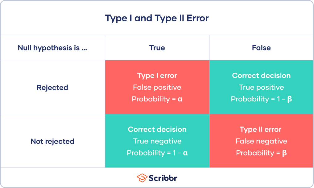
In statistics, a Type I error is a false positive conclusion, while a Type II error is a false negative conclusion.
Making a statistical decision always involves uncertainties, so the risks of making these errors are unavoidable in hypothesis testing.
The probability of making a Type I error is the significance level, or alpha (α), while the probability of making a Type II error is beta (β). These risks can be minimized through careful planning in your study design.
- Type I error (false positive): the test result says you have coronavirus, but you actually don’t.
- Type II error (false negative): the test result says you don’t have coronavirus, but you actually do.
Table of contents
- Error in statistical decision-making
- Type I error
- Type II error
- Trade-off between Type I and Type II errors
- Is a Type I or Type II error worse?
- Frequently asked questions about Type I and II errors
Error in statistical decision-making
Using hypothesis testing, you can make decisions about whether your data support or refute your research predictions with null and alternative hypotheses.
Hypothesis testing starts with the assumption of no difference between groups or no relationship between variables in the population—this is the null hypothesis. It’s always paired with an alternative hypothesis, which is your research prediction of an actual difference between groups or a true relationship between variables.
In this case:
- The null hypothesis (H0) is that the new drug has no effect on symptoms of the disease.
- The alternative hypothesis (H1) is that the drug is effective for alleviating symptoms of the disease.
Then, you decide whether the null hypothesis can be rejected based on your data and the results of a statistical test. Since these decisions are based on probabilities, there is always a risk of making the wrong conclusion.
- If your results show statistical significance, that means they are very unlikely to occur if the null hypothesis is true. In this case, you would reject your null hypothesis. But sometimes, this may actually be a Type I error.
- If your findings do not show statistical significance, they have a high chance of occurring if the null hypothesis is true. Therefore, you fail to reject your null hypothesis. But sometimes, this may be a Type II error.
A Type II error happens when you get false negative results: you conclude that the drug intervention didn’t improve symptoms when it actually did. Your study may have missed key indicators of improvements or attributed any improvements to other factors instead.
Type I error
A Type I error means rejecting the null hypothesis when it’s actually true. It means concluding that results are statistically significant when, in reality, they came about purely by chance or because of unrelated factors.
The risk of committing this error is the significance level (alpha or α) you choose. That’s a value that you set at the beginning of your study to assess the statistical probability of obtaining your results (p value).
The significance level is usually set at 0.05 or 5%. This means that your results only have a 5% chance of occurring, or less, if the null hypothesis is actually true.
If the p value of your test is lower than the significance level, it means your results are statistically significant and consistent with the alternative hypothesis. If your p value is higher than the significance level, then your results are considered statistically non-significant.
However, the p value means that there is a 3.5% chance of your results occurring if the null hypothesis is true. Therefore, there is still a risk of making a Type I error.
To reduce the Type I error probability, you can simply set a lower significance level.
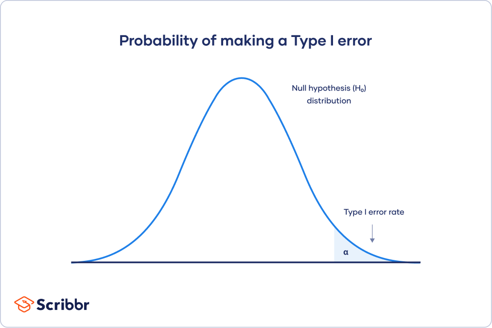
Type I error rate
The null hypothesis distribution curve below shows the probabilities of obtaining all possible results if the study were repeated with new samples and the null hypothesis were true in the population.
At the tail end, the shaded area represents alpha. It’s also called a critical region in statistics.
If your results fall in the critical region of this curve, they are considered statistically significant and the null hypothesis is rejected. However, this is a false positive conclusion, because the null hypothesis is actually true in this case!
Receive feedback on language, structure, and formatting
Professional editors proofread and edit your paper by focusing on:
- Academic style
- Vague sentences
- Grammar
- Style consistency
See an example

Type II error
A Type II error means not rejecting the null hypothesis when it’s actually false. This is not quite the same as “accepting” the null hypothesis, because hypothesis testing can only tell you whether to reject the null hypothesis.
Instead, a Type II error means failing to conclude there was an effect when there actually was. In reality, your study may not have had enough statistical power to detect an effect of a certain size.
Power is the extent to which a test can correctly detect a real effect when there is one. A power level of 80% or higher is usually considered acceptable.
The risk of a Type II error is inversely related to the statistical power of a study. The higher the statistical power, the lower the probability of making a Type II error.
However, a Type II may occur if an effect that’s smaller than this size. A smaller effect size is unlikely to be detected in your study due to inadequate statistical power.
Statistical power is determined by:
- Size of the effect: Larger effects are more easily detected.
- Measurement error: Systematic and random errors in recorded data reduce power.
- Sample size: Larger samples reduce sampling error and increase power.
- Significance level: Increasing the significance level increases power.
To (indirectly) reduce the risk of a Type II error, you can increase the sample size or the significance level.
Type II error rate
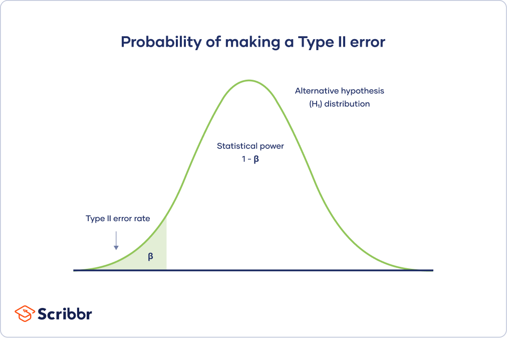
The alternative hypothesis distribution curve below shows the probabilities of obtaining all possible results if the study were repeated with new samples and the alternative hypothesis were true in the population.
The Type II error rate is beta (β), represented by the shaded area on the left side. The remaining area under the curve represents statistical power, which is 1 – β.
Increasing the statistical power of your test directly decreases the risk of making a Type II error.
Trade-off between Type I and Type II errors
The Type I and Type II error rates influence each other. That’s because the significance level (the Type I error rate) affects statistical power, which is inversely related to the Type II error rate.
This means there’s an important tradeoff between Type I and Type II errors:
- Setting a lower significance level decreases a Type I error risk, but increases a Type II error risk.
- Increasing the power of a test decreases a Type II error risk, but increases a Type I error risk.
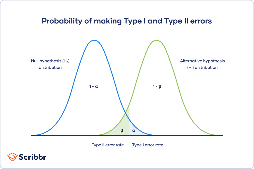
This trade-off is visualized in the graph below. It shows two curves:
- The null hypothesis distribution shows all possible results you’d obtain if the null hypothesis is true. The correct conclusion for any point on this distribution means not rejecting the null hypothesis.
- The alternative hypothesis distribution shows all possible results you’d obtain if the alternative hypothesis is true. The correct conclusion for any point on this distribution means rejecting the null hypothesis.
Type I and Type II errors occur where these two distributions overlap. The blue shaded area represents alpha, the Type I error rate, and the green shaded area represents beta, the Type II error rate.
By setting the Type I error rate, you indirectly influence the size of the Type II error rate as well.
It’s important to strike a balance between the risks of making Type I and Type II errors. Reducing the alpha always comes at the cost of increasing beta, and vice versa.
Is a Type I or Type II error worse?
For statisticians, a Type I error is usually worse. In practical terms, however, either type of error could be worse depending on your research context.
A Type I error means mistakenly going against the main statistical assumption of a null hypothesis. This may lead to new policies, practices or treatments that are inadequate or a waste of resources.
In contrast, a Type II error means failing to reject a null hypothesis. It may only result in missed opportunities to innovate, but these can also have important practical consequences.
Frequently asked questions about Type I and II errors
-
How do you reduce the risk of making a Type I error?
-
The risk of making a Type I error is the significance level (or alpha) that you choose. That’s a value that you set at the beginning of your study to assess the statistical probability of obtaining your results (p value).
The significance level is usually set at 0.05 or 5%. This means that your results only have a 5% chance of occurring, or less, if the null hypothesis is actually true.
To reduce the Type I error probability, you can set a lower significance level.
-
What is statistical significance?
-
Statistical significance is a term used by researchers to state that it is unlikely their observations could have occurred under the null hypothesis of a statistical test. Significance is usually denoted by a p-value, or probability value.
Statistical significance is arbitrary – it depends on the threshold, or alpha value, chosen by the researcher. The most common threshold is p < 0.05, which means that the data is likely to occur less than 5% of the time under the null hypothesis.
When the p-value falls below the chosen alpha value, then we say the result of the test is statistically significant.
-
What is statistical power?
-
In statistics, power refers to the likelihood of a hypothesis test detecting a true effect if there is one. A statistically powerful test is more likely to reject a false negative (a Type II error).
If you don’t ensure enough power in your study, you may not be able to detect a statistically significant result even when it has practical significance. Your study might not have the ability to answer your research question.
Cite this Scribbr article
If you want to cite this source, you can copy and paste the citation or click the “Cite this Scribbr article” button to automatically add the citation to our free Citation Generator.
Bhandari, P.
(2022, November 11). Type I & Type II Errors | Differences, Examples, Visualizations. Scribbr.
Retrieved February 9, 2023,
from https://www.scribbr.com/statistics/type-i-and-type-ii-errors/
Is this article helpful?
You have already voted. Thanks 
Your vote is saved
Processing your vote…
In any experiment that is carried out, we often rely on probabilities to prove (or disprove) a hypothesis.
When carrying out an A/B test, for example, we are often seeking statistically significant results.
We are great advocates of testing in production and so A/B testing is one effective way to test your features on a select number of users to make sure that they’re working as they should before rolling them out to everyone else.
However, since such tests are always based on probabilities, as no hypothesis testing can be 100% certain, this is why sometimes we may arrive at wrong conclusions leading to what is known as type I and type II errors.
Statistical significance
We mentioned the term ‘statistical significance’ which is what any experiment is seeking to find. In the experiments you run, you want to make sure that a relationship actually exists between the variables proposed in your hypothesis, which is the purpose of an A/B test.
You are ultimately seeking to ensure that your A/B tests achieve statistical significance before making any decisions.
If you’ve often carried out A/B tests, then you’re probably familiar with this term as it gives you the tools necessary to make informed decisions to meet your business goals.
For the sake of further clarification, a statistically significant result in such tests means that the result is highly unlikely to have occurred randomly and is instead attributed to a specific cause or trend.
Simply put, it is the probability that the gap or difference between variations and control is not random or due to chance but due to a well-backed experiment. It indicates your risk tolerance and confidence level.
In other words, when you run an A/B test with a 95% significance or confidence level, this means you can be 95% confident that when you determine the winning variation, the results obtained are real and not due to chance.
However, as with any hypothesis test based on statistics and probabilities, two types of errors can show up in your results.
Hypothesis testing
Before we delve deeper into type I errors, it would be worthwhile to give an overview of what hypothesis testing is.
Hypothetical testing is when a hypothesis is tested against its opposite to determine whether it’s true or not. In this case, you have the null hypothesis and the alternative hypothesis or two variables.
Therefore, a statistical hypothesis test is used to determine a possible conclusion from two different and conflicting hypotheses.
The null hypothesis posits that there is no relationship between the two proposed phenomen while the alternative hypothesis is the opposite of what is stated in the null hypothesis.
P-values used in statistical testing help decide whether to reject the null hypothesis. The smaller the value, the more likely you are to reject the null hypothesis. In other words, it tells you how likely your data would have occurred under the null hypothesis.
The p-value is most commonly set at p< 0.05 to declare statistical significance.
However, in any statistical test, there is always a degree of uncertainty so the risks of committing an error are quite high.
The following table depicts these errors in relation to the null hypothesis:

Type 1 error
One such error is type 1 (or type I) error, also referred to as false positive, which is the wrong rejection of a null hypothesis even though it’s true. In other words, you conclude that the results are statistically significant when they are simply a result of chance or due to unrelated factors.
Simply put, a type 1 error occurs when the tester validates a statistically significant difference when there isn’t one.
In an A/B test, a type 1 error is when you declare a bad variation as the winner even though the test conducted was inconclusive. In other words, as a false positive, you adhere to the belief that a variation in a test has made a statistically significant difference.
Type 1 errors have a probability of “α” or alpha correlated to the confidence level you set. For example, if you set a confidence level of 95% then there is a 5% chance that you will get a type 1 error.
Consequence of type 1 errors
Type 1 means wrongfully assuming that your hypothesis testing worked even though it hasn’t. Consequently, the main reason to remain on the lookout for such errors is that they may end up costing your company a lot of money as they could possibly lead to loss in sales.
If, for example, you tested out a change in the color of a button on your homepage and you noticed early on that the button did lead to more clicks. You are then convinced that this variation made a difference so you decide to end the test early by wrongfully concluding that there is indeed a correlation between this change in color and conversion rates.
Thus, you end up deploying this variation to all your users to find that, surprise, it didn’t actually have an impact. The end result is that you could risk hurting your customer conversion rate in the long run.
The best way to avoid such errors may be to increase test duration to ensure that your variation outperformed the control in the long run and sample size.
Related: Sample Size Calculator for A/B Testing
Type 2 error
Type 2 (or type II) errors, also referred to as false negatives, occur when you don’t reject the null hypothesis when it’s actually false and you end up rejecting your own hypothesis and variation. Type 2 errors have a probability of β or beta.
In an A/B test, this means that you fail to conclude there was an effect when there indeed was and so no conclusive winner is declared among the control and variations even though there should be one.
In other words, you believe that a variation has made no statistical difference and you mistakenly believe the null hypothesis and that a relationship doesn’t exist when it does.
A type 2 error is inversely related to the statistical power of a test, where power is the probability that a test can detect an effect that actually exists. The higher the statistical power, the lower the probability of committing a type 2 error.
Statistical power usually depends on three factors: sample size, significance level and The “true” value of your tested parameter.
Consequence of type 2 errors
Just like type I errors, type II errors can lead to false assumptions and poor decision making by concluding the test too early.
Furthermore, getting false negatives and failing to notice the effect of your variations may lead to wasted opportunities as you’re not taking advantage of opportunities to increase your conversion rate.
To reduce the risk of such an error, make sure you increase the statistical power of your test, for example, having a big enough sample size. This would entail gathering more data over a longer period of time to help avoid reaching the false conclusion that your experiment didn’t have an impact when the opposite is true.
The probability of making type I and type II errors is depicted in the image below, where the null hypothesis distribution shows all possible results if the null hypothesis is true while the alternative hypothesis shows all possible results if the alternative hypothesis is true:

As can be seen, type I and type II errors occur where these two distributions overlap.
Let’s sum up…
Let’s consider these two scenarios:
- If your results demonstrate statistical significance, this means that there is a difference between the variations. In that case you may reject the null hypothesis. However, this could sometimes be a type 1 error.
- If your results don’t show statistical significance then the null hypothesis cannot be rejected. This could also sometimes be a type 2 error.
In the end, it’s important to strike a balance between making type 1 and type 2 errors. Many argue that making type I errors may be more damaging as it could lead to changes that will end up wasting resources, costing time and money while type 2 errors are more about ‘missed opportunities’ (though it could also have significant consequences).
The essential thing to remember is that A/B tests are based on statistical probabilities meaning that the results obtained are never 100% certain.
Nevertheless, these tests serve as a valuable tool to help marketers increase sales and conversion rate so even if your results may not be as certain as you’d like them to be, you can still increase the probability of the test result being true by avoiding the aforementioned errors.
To reduce probabilities for error, the key is to increase sample size and run the test for as long as possible to ensure the collection of as accurate as possible data and to increase the credibility of your test results.
Read more about A/B testing statistics in our A/B testing guide here.
Info
